$SL(2,7)$ Representations and their relevance to Neutrino Physics

G. Aliferis^a , G. K. Leontaris^b,c and N. D. Vlachos^a

^a Department of Nuclear and Particle Physics

University of Thessaloniki

GR-54124 Thessaloniki, Greece

^bPhysics Department, University of Ioannina

GR-45110 Ioannina, Greece

^c Department of Physics, CERN

CH-1211, Geneva 23, Switzerland

The investigation of the rôle of finite groups in flavor physics and particularly, in the interpretation of the neutrino data has been the subject of intensive research. Motivated by this fact, in this work we derive the three-dimensional unitary representations of the projective linear group $PSL_{2}(7)$. Based on the observation that the generators of the group exhibit a latin square pattern, we use available computational packages on discrete algebra to determine the generic properties of the group elements. We present analytical expressions and discuss several examples which reproduce the neutrino mixing angles in accordance with the experimental data.

1 Synopsis

Abelian and non-abelian discrete symmetries have been extensively used to impose constraints on the Yukawa lagrangian. In model building they are often used to generate hierarchical structures in the fermion mass matrices, to eliminate proton decay operators and suppress other terms inducing unobserved processes. The structure of the neutrino mass matrix and the experimentally measured mixing angles in particular, hint to the existence of an underlying non-Abelian flavor symmetry. In this context, the neutrino mass matrix is assumed to be invariant under certain transformations of the discrete group $D_{f}$ (for reviews see [1, 2, 3]). Therefore, in unified theories of the fundamental gauge interactions the symmetry of the effective model is expected to contain a non-abelian gauge group $G_{GUT}$ accompanied by a (non)-abelian discrete flavor symmetry $D_{f}$. In some string scenarios the total effective symmetry $G_{GUT}\times D_{f}$ is usually embedded in a higher unified group, such as $E_{8}$ [4]. For the most familiar GUT symmetries such as $E_{6},SO(10)$ and $SU(5)$, the discrete group is a subgroup of $SU(3)$. In the past, several of these cases have been considered, including those belonging to the chains $S_{n},A_{n}$ and possess triplet representations. In the present work we focus on some particular cases of a general class of discrete symmetries. These are the special linear groups $SL_{2}(p)$ [5, 6] and their corresponding projective ones, $PSL_{2}(p)$, with $p$ prime number. From this class of groups it is sufficient for our purposes to take $p\leq 7$ since these are the only cases where the resulting discrete groups contain triplet representations and at the same time are embedded in $SU(3)$. Moreover, from the physics point of view, the rather interesting case of $PSL_{2}(7)$ which is a simple subgroup of $SU(3)$, is less explored (see however [7, 8, 9]), and it is our main focus in the present work. Since we demand invariance of the neutrino mass matrix under certain group actions, a prerequisite for such an analysis is the explicit form of the group elements of $PSL_{2}(7)$. However, while finding the representations of the elements and the multiplication tables of $A_{3},A_{4},A_{5}$ is relatively easy, this becomes an onerous process for $PSL_{2}(7)$.

In a previous work [10], using the automorphisms of the discrete and finite Heisenberg group, the 3-dimensional representations of the $PSL_{2}(p)$ generators were constructed. It is our purpose here to systematically derive the structure of all the elements of the three-dimensional representations of $PSL_{2}(7)$. The explicit form of the three-dimensional unitary representations would be a very useful tool in many physics applications including their possible relevance to the structure of the neutrino mass matrix and lepton mixing angles. Focusing on neutrino physics, a usual approach is to construct neutrino and charged lepton mass matrices invariant under certain elements of the assumed group. Hence, a systematic exploration of the specific properties and in particular the characteristic mixing matrix of the neutrino sector require such a methodology.

Finite groups were proposed long time ago as a possible symmetry to the peculiar neutrino hierarchy and this is our basic motivation for the present construction. With many details found in reviews and other works, here, we only give a brief description of our assumptions. We consider a scenario where the charged lepton and neutrino mass matrices are subject to constraints under the same or different subgroups of a covering parent discrete symmetry. This is compatible, for example, with model building in string theory framework. Taking for example the $SU(5)$ gauge theory, in some F-theory framework, the trilinear Yukawa couplings for the various types of fields are realized at different points of the internal manifold and they correspond to different symmetry enhancements of the $SU(5)$ singularity [11]. For example, the $10\cdot 10\cdot 5$ coupling is realized at a ‘point’ of the compact manifold associated with $E_{6}$ enhancement and the $10\cdot\bar{5}\cdot\bar{5}$ at an $SO(12)$ enhancement. Similarly, the corresponding discrete symmetry associated with these points may differ, although they could be subgroups of the same covering discrete group. We assume that this is the case for $m_{\ell}$ and $m_{\nu}$ which are not realized at the same ‘point’. Then, we consider that the neutrino mass matrix commutes with an element $A$ of a given discrete group

$$[m_{\nu},A]=0\,,$$ (1)

while a similar relation holds for the charged lepton mass matrix, as well. Then, the vanishing of the commutator (1) implies that both, $m_{\nu}$ and $A$ have a common system of eigenvectors, hence they define the diagonalising (mixing) matrix $V_{\nu}$. In other words, $U_{\nu}^{\dagger}AU_{\nu}=A^{diag.}$ as well as $U_{\nu}^{\dagger}m_{\nu}U_{\nu}=m_{\nu}^{diag.}$.

The layout of the article is as follows. In section section 2 we summarize the basic steps of the generators construction  [10] using the work of [12]. In section 3, based on the observation that the $PSL_{2}(7)$ 3-d representations exhibit a specific structure, we calculate the elements of the three-dimensional representation. In section 4 we discuss its possible relevance to neutrino physics and present several working examples. We summarize our results in section 5.

2 The three-dimensional representations of the $PSL_{2}(7)$ group

In the present section we describe the basic steps for the construction of the unitary representations of the $PSL_{2}(p)$ group. This is defined by the $2\times 2$ matrices $\mathfrak{a}$ with elements integers modulo $p$, where $p$ is a prime number, and determinant equal to one modulo $p$:

$$\mathfrak{a}=\left(\begin{array}[]{cc}a&b\\ c&d\end{array}\right),\;a,b,c,d\in\mathbb{Z}_{p},\;{\rm det}\mathfrak{a}=1\,{\rm mod}{\,p}$$ (2)

The elements of the group can be constructed from combinations of powers of two generators denoted here with $\mathfrak{a},\mathfrak{b}$, which, in a specific representation are defined by the matrices

$$\mathfrak{a}=\left(\begin{array}[]{cc}0&-1\\ 1&0\end{array}\right)\,;\;\mathfrak{b}=\left(\begin{array}[]{cc}0&-1\\ 1&1\end{array}\right)\,\cdot$$ (7)

These satisfy the relations

$$\mathfrak{a}^{2}=\mathfrak{b}^{3}=-I\equiv-{\left(\begin{array}[]{cc}{1}&0\\ 0&{1}\end{array}\right)}\,\cdot$$ (8)

To define the projective linear group $PSL_{2}(p)$, we first observe that $SL_{2}(p)$ contains a normal subgroup of two elements, $Z_{2}=\{I,-I\}$. The $PSL_{2}(p)$ is defined as the quotient subgroup, by identifying the unit matrix $I$ with $-I$

$$PSL_{2}(p)=SL_{2}(p)/\{I,-I\}\;\cong\;SL_{2}(p)/Z_{2}$$ (9)

Next, we use Weil’s metaplectic representation $U(A)$ derived long time ago by Balian and Itzykson [12], ( see also [13]) to construct the $p$-dimensional unitary representations of $SL_{2}(p)$ groups. The explicit form of $U(A)$ is given in terms of the elements $a,b,c,d$ of the $2\times 2$ matrix (2) as follows

$${U(A)}={\frac{\sigma(1)\sigma({\delta})}{p}}\sum_{r,s}{\omega}^{[b{r}^{2}+(d-a){rs}-c{s}^{2}]/(2{\delta})}{J_{r,s}}$$ (10)

for ${\delta}={2-a-d}\neq 0$. For $\delta=0$, we distinguish the following cases:

$${\delta}=0,\;b\neq 0: U(A)=\frac{\sigma(-2b)}{\sqrt{p}}\sum_{s}\omega^{s^{2}/(2b)}{J_{s(a-1)/b,s}}$$

$${\delta}={b}=0,\;c\neq 0: U(A)=\frac{\sigma(2c)}{\sqrt{p}}\sum_{r}\omega^{-r^{2}/(2c)}{P^{r}}$$ (11)

$${\delta}={b}=0=c=0: {U(1)=I}$$

A few clarifications on notation and definitions in the above formulae are needed.

The quantities $J_{r,s},J_{s(a-1)/b,s}$ are defined as follows

$$J_{n_{1},n_{2}}\equiv J_{\vec{n}}=\omega^{\frac{n_{1}n_{2}}{2}}P^{n_{1}}Q^{n_{2}}~{},$$ (12)

where $\omega=e^{2\pi i/p}$ is the $p^{th}$ root of unity, while $P,Q$ are position and momentum operators with elements $P_{kl}=\delta_{k-1,l}$ and, $Q_{kl}=\omega^{k}\delta_{kl}$ repsectively. The generators (12) obey the ‘multiplication’ law

$${J_{\vec{m}}J_{\vec{n}}}={\omega}^{\frac{\vec{n}\times\vec{m}}{2}}{J_{\vec{m}+\vec{n}}}$$

and constitute a subset of the Heisenberg group [12].

The quantities $\sigma(a)$ and $\left({\frac{a}{p}}\right)$, are the Quadratic Gauss Sum and the Legendre symbol respectively. These are defined as follows:

$${\sigma(a)} = \frac{1}{\sqrt{p}}\,\sum_{k=0}^{p-1}\omega^{ak^{2}}=\left({\frac{a}{p}}\right)\times\left\{\begin{array}[]{cc}1&{\rm for}\,p=4k+1\\ i&{\rm for}\,p=4k-1\end{array}\right.$$ (15)

and

$$\left({\frac{a}{p}}\right) = \left\{\begin{array}[]{cc}0&{\rm if}{a}\;{\rm devides}\;{p}\\ +1&{\rm if}\;{a}={\cal QR}\;{p}\\ -1&{\rm if}\;{a}\neq{\cal QR}\;{p}\end{array}\right.$$ (19)

where ${\cal QR}$ means Quadratic Residue .

The so obtained $p$-dimensional representation decomposes into two irreducible unitary representations of dimensions $\frac{p+1}{2}$ and $\frac{p-1}{2}$. These are discrete subgroups of the unitary groups $SU(\frac{p\pm 1}{2})$ and for $p=7$ we obtain the 3-dimensional representation of the discrete group $PSL_{2}(7)$ which is a subgroup of $SU(3)$. Smaller $p$ values result to $A_{3}$ and $A_{5}$ groups which have been extensively studied, while the next value of $p=11$ results to $PSL_{2}(11)$ which does not contain triplet representations in its decompositions $(p=11=6+5)$, therefore it is not of our primary interest.

The $SL_{2}(p)$ group with $p$ prime has $p(p^{2}-1)$ elements and the corresponding projective $PSL_{2}(p)$ contains half of them. Therefore, the $PSL_{2}(7)$ has $168$ elements and it is a simple discrete subgroup of $SU(3)$. Using the method described above we can construct [10] the three-dimensional representations of $PSL_{2}(7)$, satisfying the conditions

$$\mathfrak{a}^{2}=\mathfrak{b}^{3}=(\mathfrak{ab})^{7}=[\mathfrak{a},\mathfrak{b}]=1$$ (20)

where the ‘commutator’ for the group elements is defined as usual: $[\mathfrak{a},\mathfrak{b}]=\mathfrak{a}^{-1}\mathfrak{b}^{-1}\mathfrak{ab}$. The generators of the 3-dimensional unitary representation of the $PSL_{2}(7)$ group, associated with ${\mathfrak{\mathfrak{a}}}$ and ${\mathfrak{\mathfrak{b}}}$ of (2) can be written in terms of the $7^{th}$ root of unity ${\eta}=e^{2\pi i/{7}}$, as follows:

$${A_{[3]}} = {\frac{i}{\sqrt{7}}\left(\begin{array}[]{ccc}{\eta}^{2}-{\eta}^{5}&{\eta}^{6}-{\eta}&{\eta}^{3}-{\eta}^{4}\\ {\eta}^{6}-{\eta}&{\eta}^{4}-{\eta}^{3}&{\eta}^{2}-{\eta}^{5}\\ {\eta}^{3}-{\eta}^{4}&{\eta}^{2}-{\eta}^{5}&{\eta}-{\eta}^{6}\end{array}\right)}$$ (24)

and

$${B_{[3]}} = {\frac{i}{\sqrt{7}}\left(\begin{array}[]{ccc}{\eta}-{\eta}^{4}&{\eta}^{4}-{\eta}^{6}&{\eta}^{6}-1\\ {\eta}^{5}-1&{\eta}^{2}-{\eta}&{\eta}^{5}-{\eta}\\ {\eta}^{2}-{\eta}^{3}&1-{\eta}^{3}&{\eta}^{4}-{\eta}^{2}\end{array}\right)}\,.$$ (28)

It can be readily checked that these satisfy the required relations:

$${A_{[3]}}^{2}={B_{[3]}}^{3}=({A_{[3]}B_{[3]}})^{7}=[{A_{[3]},B_{[3]}}]^{4}=I~{}\cdot$$ (29)

Implementing the above method, we can find the $PSL_{2}(7)$ group elements, imposing the appropriate conditions on products of powers of $2\times 2$ matrices given in (2) and then using the metaplectic representation to build the 3-dimensional representations of $PSL_{2}(7)$. However, in this section we will follow a different approach which, in our opinion, reveals some new and very interesting properties of the group elements.

For all practical purposes however, it suffices to take the two generators and explicitly construct all the elements of the three-dimensional unitary representations of $PSL_{2}(7)$ using the GAP system for computational discrete algebra available in the web[14]. After some algebra it can be shown that the two generators can be written as

$$A_{[3]}=\begin{bmatrix}\rho_{1}&-\rho_{2}&-\rho_{3}\\ -\rho_{2}&\rho_{3}&\rho_{1}\\ -\rho_{3}&\rho_{1}&\rho_{2}\end{bmatrix}\,,\;\;B_{[3]}=\begin{bmatrix}\rho_{1}\eta^{-1}&\rho_{2}\eta^{\frac{3}{2}}&\rho_{3}\eta^{-\frac{1}{2}}\\ \rho_{2}\eta^{\frac{5}{2}}&\rho_{3}\eta^{-2}&\rho_{1}\eta^{3}\\ \rho_{3}\eta^{\frac{5}{2}}&\rho_{1}\eta^{-2}&\rho_{2}\eta^{3}\end{bmatrix}~{}\cdot$$ (30)

where

$$\rho_{1}=-\frac{2}{\sqrt{7}}\cos\frac{\pi}{14},\;\rho_{2}=-\frac{2}{\sqrt{7}}\cos\frac{3\pi}{14},\;\rho_{3}=-1-\rho_{1}-\rho_{2}~{}\cdot$$ (31)

The quantities $\rho_{1},\rho_{2},\rho_{3}$ satisfy the cubic equation

$$x^{3}+x^{2}-\frac{1}{7}=0~{},$$

and the relation $\rho_{2}=7\rho_{1}^{3}-3\rho_{1}~{}$.

We now observe that the moduli of the elements of both matrices follow a latin square pattern [15]. The so found group matrices can be classified according to their conjugacy class as shown in Table 1.

Order	character	$\#$	Tag
${2}$	$-1$	$21$	$el_{2}$
${3}$	$\hskip 7.82433pt0$	$56$	$el_{3}$
${4}$	$+1$	$42$	$el_{4}$
${7}$	$-\frac{1}{2}\pm i\frac{\sqrt{7}}{2}$	$48$	$el_{7}$

Table 1: The order, character, and the number of elements of the conjugacy classes of $PSL_{2}(7)$

3 On the properties of the representation matrices

In this section we investigate useful properties of latin square matrices in view of their relation to the $PSL_{2}(7)$ elements. We start with the $3\times 3$ case with real entries. These are of the following two types

$$M_{1}=\begin{bmatrix}r_{1}&r_{2}&r_{3}\\ r_{2}&r_{3}&r_{1}\\ r_{3}&r_{1}&r_{2}\end{bmatrix},\;M_{2}=\begin{bmatrix}r_{1}&r_{2}&r_{3}\\ r_{3}&r_{1}&r_{2}\\ r_{2}&r_{3}&r_{1}\end{bmatrix}\,,$$ (32)

and their permutations. From these two, only the first type appears in $PSL_{2}\left(7\right)$. The orthogonality condition $M_{1}^{2}=1$ implies that

$$r_{1}^{2}+r_{2}^{2}+r_{3}^{2}=1,\;r_{1}r_{2}+r_{1}r_{3}+r_{2}r_{3}=0$$ (33)

while requiring $\det M_{1}=1$ we get

$$r_{1}+r_{2}+r_{3}=-1\cdot$$ (34)

Thus, if the matrix $M_{1}$ is part of an irreducible group representation, it should belong to the conjugacy class $el_{2}$ with character $-1$. Notice that $r_{1},r_{2},r_{3}$ satisfy the algebraic equation

$$x^{3}+x^{2}-q=0,\;{\rm where}\;q=r_{1}r_{2}r_{3},$$ (35)

and the reality of the roots requires that ${\small 0<q<\frac{4}{27}}\cdot$ For the case of $PSL_{2}(7)$, $q=\frac{1}{7}<\frac{4}{27}\cdot$

The obvious generalization includes complex elements and takes the form

$$M=\begin{bmatrix}r_{1}e^{\imath c_{1}}&r_{2}e^{\imath c_{2}}&r_{3}e^{\imath c_{3}}\\ r_{2}e^{\imath c_{4}}&r_{3}e^{\imath c_{5}}&r_{1}e^{\imath c_{6}}\\ r_{3}e^{\imath c_{7}}&r_{1}e^{\imath c_{8}}&r_{2}e^{\imath c_{9}}\end{bmatrix}~{}.$$ (36)

Unitarity and the condition det$M=1$ restrict the number of free parameters $r_{i},c_{i}$. The conditions (33,34) still hold, and the final form is

$$M=\begin{bmatrix}r_{1}e^{ic_{1}}&r_{2}e^{ic_{2}}&r_{3}e^{ic_{3}}\\ r_{2}e^{i\left(c_{1}-c_{2}+c_{5}\right)}&r_{3}e^{ic_{5}}&r_{1}e^{i\left(c_{3}-c_{2}+c_{5}\right)}\\ r_{3}e^{-i\left(c_{3}+c_{5}\right)}&r_{1}e^{i\left(c_{2}-c_{3}-c_{1}-c_{5}\right)}&r_{2}e^{-i\left(c_{1}+c_{5}\right)}\end{bmatrix}\cdot$$ (37)

Looking more closely at the $PSL_{2}(7)$ elements constructed by GAP, we observe that a great number of them can be written in this form when we substitute $\rho_{1},\rho_{2},\rho_{3}$ given in (31) in place of $r_{1},r_{2},r_{3}$ and all the phases are closely related to the set of the seventh roots of unity. The secular equation for $M$ reads

$$x^{3}-tr\left(M\right)x^{2}+trM^{\ast}x-1=0~{}\cdot$$ (38)

It can be readily checked that given the character of the conjugacy class Tr$\left(M\right)$, the secular equation (38) reproduces the correct eigenvalues of the representation matrices. For example, the order seven elements character is Tr$M=-\frac{1}{2}-i\frac{\sqrt{7}}{2}$ and solving the secular equation we find the eigenvalues

$$\exp\left[\frac{10\pi i}{7}\right],\;\exp\left[\frac{6\pi i}{7}\right],\;\exp\left[\frac{12\pi i}{7}\right],$$ (39)

in accordance to the group elements table. For the order two elements a trivial calculation implies that $c_{1}=c_{5}=0$ giving a general form

$$M=\begin{bmatrix}r_{1}&r_{2}e^{\imath c_{2}}&r_{3}e^{\imath c_{3}}\\ r_{2}e^{-\imath c_{2}}&r_{3}&r_{1}e^{\imath\left(c_{3}-c_{2}\right)}\\ r_{3}e^{-\imath c_{3}}&r_{1}e^{\imath\left(c_{2}-c_{3}\right)}&r_{2}\end{bmatrix}~{}\cdot$$ (40)

Next, for the general matrix $M$, information on the allowed values for $c_{1}$ and $c_{5}$ can be extracted by taking the system of equations

$$r_{1}e^{ic_{1}}+r_{2}e^{-i(c_{1}+c_{5})}+r_{3}e^{ic_{5}} = {\rm Tr}M$$ (41)

$$r_{1}+r_{2}+r_{3} = -1$$ (42)

$$r_{1}r_{2}+r_{2}r_{3}+r_{3}r_{1} = 0$$ (43)

and substituting the character ${\rm Tr}M$ of the corresponding conjugacy class. Parametrizing the phases as

$$c_{1}=\frac{2\pi}{7}n,\;c_{5}=\frac{2\pi}{7}m$$ (44)

and taking $q=r_{1}r_{2}r_{3}=\frac{1}{7}$ we get only integer values for $n,m$. These values are symmetric under the interchange of $m$ and $n$. Notice that the value, $q=\frac{1}{7}$ identifies $r_{1}\allowbreak,r_{2},r_{3}$ with $\rho_{1},\rho_{2},\rho_{3}$ respectively.

Solving the system of equations (41)-(43), for the order $3$ elements we have

$$\begin{bmatrix}r_{1}\\ r_{2}\\ r_{3}\end{bmatrix}=\begin{bmatrix}1&1&1\\ \cos c_{1}&\cos\left(c_{1}+c_{5}\right)&\cos c_{5}\\ \sin c_{1}&-\sin\left(c_{1}+c_{5}\right)&\sin c_{5}\end{bmatrix}^{-1}\begin{bmatrix}-1\\ 0\\ 0\end{bmatrix}~{},$$ (45)

and the solutions found are

−5−3−4−2−2−114−51−45−2312−54−31−1324−4−1−32−1535⋅\begin{tabular}[c]{rrrrrrrr}$\mathbf{c}_{1}$&$\mathbf{c}_{5}$&$\mathbf{c}_{1}$&$\mathbf{c}_{5}$&$\mathbf{c}_{1}$&$\mathbf{c}_{5}$&$\mathbf{c}_{1}$&$\mathbf{c}_{5}$\\ $\mathbf{n}$&$\mathbf{m}$&$\mathbf{n}$&$\mathbf{m}$&$\mathbf{n}$&$\mathbf{m}$&$\mathbf{n}$&$\mathbf{m}$\\ \hline\cr$-5$&$-3$&$-4$&$-2$&$-2$&$-1$&$1$&$4$\\ $-5$&$1$&$-4$&$5$&$-2$&$3$&$1$&$2$\\ $-5$&$4$&$-3$&$1$&$-1$&$3$&$2$&$4$\\ $-4$&$-1$&$-3$&$2$&$-1$&$5$&$3$&$5$\\ \end{tabular}\ ~{}\cdot

c1c5c1c5c1c5c1c5nmnmnmnm

For the order 4 elements we have

$$\begin{bmatrix}r_{1}\\ r_{2}\\ r_{3}\end{bmatrix}=\begin{bmatrix}1&1&1\\ \cos c_{1}&\cos\left(c_{1}+c_{5}\right)&\cos c_{5}\\ \sin c_{1}&-\sin\left(c_{1}+c_{5}\right)&\sin c_{5}\end{bmatrix}^{-1}\begin{bmatrix}-1\\ 1\\ 0\end{bmatrix}~{},$$ (46)

which imply the following values for $m,n$ and $c_{1,5}$

$$\mathbf{c}_{1}$$

For the order $7$ elements we have

$$\begin{bmatrix}r_{1}\\ r_{2}\\ r_{3}\end{bmatrix}=\begin{bmatrix}1&1&1\\ \cos c_{1}&\cos\left(c_{1}+c_{5}\right)&\cos c_{5}\\ \sin c_{1}&-\sin\left(c_{1}+c_{5}\right)&\sin c_{5}\end{bmatrix}^{-1}\begin{bmatrix}-1\\ -\frac{1}{2}\\ -\frac{\sqrt{7}}{2}\end{bmatrix}~{}\cdot$$ (47)

The solutions are

$$\mathbf{c}_{1}$$

Note that all these solutions when applied to the system for $r_{1},r_{2},r_{3}$ just generate permutations of the root system $\rho_{1},\rho_{2},\rho_{3}$. Concerning the possible values of the remaining phases $c_{2}$ and $c_{3}$ no further information can be extracted without using the group algebra.

4 $SL_{2}(7)$ invariance and the neutrino mixing matrix

Neutrino oscillations are associated with the existence of non-zero masses $m_{\nu_{i}}$ and non-zero $\theta_{ij}$ mixing angles in the lepton sector. In a standard parametrization the corresponding lepton mixing matrix is given by the expression

$$U=U_{l}^{\dagger}U_{\nu}=\left(\begin{array}[c]{lll}c_{12}c_{13}&c_{13}s_{12}&s_{13}e^{-i\delta}\\ -c_{23}s_{12}-c_{12}s_{13}s_{23}e^{i\delta}&c_{12}c_{23}-s_{12}s_{13}s_{23}e^{i\delta}&c_{13}s_{23}\\ s_{12}s_{23}-c_{12}c_{23}s_{13}e^{i\delta}&-c_{23}s_{12}s_{13}-c_{12}s_{23}e^{i\delta}&c_{13}c_{23}\end{array}\right)$$ (48)

where, to avoid clutter, we have denoted $c_{ij}\equiv\cos\theta_{ij}$ and $s_{ij}\equiv\sin\theta_{ij}$. The $3\sigma$ range of the three mixing angles in accordance with recent data, is given by

$$\sin^{2}\theta_{12}=[0.25-0.35],\;\sin^{2}\theta_{23}=[0.38-0.62],\;\sin^{2}\theta_{13}=[0.0185-0.0246]\cdot$$ (49)

We will confront our results on the masses and mixing matrices with the experimental data.

In order to construct the mixing matrices one has to first assume the symmetries of the neutrino and charged leptons mass matrices. These symmetries are connected to the elements of $PSL_{2}\left(7\right)$ which leave the mass matrices invariant (i.e. vanishing commutator). Then we determine the diagonalizing matrices $U$ for these elements. Note that the diagonalizing matrices are not uniquely defined since there are $3!$ ways to arrange the eigenvalues in the resulting diagonal matrices. Since $PSL_{2}\left(7\right)$ contains four conjugacy classes characterized by elements of order $2$ $\left(el_{2}\right)$, order $3$ $\left(el_{3}\right)$, order $4$ $\left(el_{4}\right)$, and $7$ $\left(el_{7}\right)$ (see appendix for notation), in order to construct the mixing matrices one has to combine the diagonalizing matrices in all possible ways. This search of course can only be done numerically. In order to conform with experimental data we kept only the cases where $0.136<\left|U_{13}\right|<0.157$, $0.499<\left|U_{12}\right|<0.595$, $0.615<\left|U_{23}\right|<0.785$. It turns out that the only symmetry for the neutrino mass matrix that is compatible with data is connected to a number of order $2$ elements. For the charged leptons mass matrix the symmetry allowed is connected to both order $3$ and order $7$ elements. The results are shown in the tables 2 and 3. Obviously, these tables should also contain the inverse elements. Since the order $2$ elements equal their inverses and the rest can be easily calculated, the inverses are not shown for reasons of clarity.

$\mathbf{el}_{2}$	$\mathbf{el}_{3}$	$\mathbf{el}_{3}$	$\mathbf{el}_{3}$	$\mathbf{el}_{3}$	$\mathbf{el}_{3}$	$\mathbf{el}_{3}$	$\mathbf{el}_{3}$	$\mathbf{el}_{3}$
$15$	$6$	$7$	$15$	$17$	$23$	$25$	$37$	$41$
$16$	$5$	$6$	$19$	$21$	$24$	$26$	$39$	$42$
$17$	$4$	$5$	$16$	$18$	$25$	$27$	$38$	$41$
$18$	$3$	$4$	$15$	$20$	$26$	$28$	$40$	$42$
$19$	$1$	$3$	$17$	$19$	$22$	$27$	$36$	$38$
$20$	$1$	$8$	$16$	$21$	$23$	$28$	$37$	$40$
$21$	$7$	$8$	$18$	$20$	$22$	$24$	$36$	$39$

Table 2: Solutions for the charged lepton mass matrix in terms of the order 3 elements.

$\mathbf{el}_{2}$	$\mathbf{el}_{7}$	$\mathbf{el}_{7}$	$\mathbf{el}_{7}$	$\mathbf{el}_{7}$	$\mathbf{el}_{7}$	$\mathbf{el}_{7}$
$8$	$3$	$5$	$15$	$16$	$21$	$24$
$9$	$1$	$2$	$17$	$18$	$22$	$25$
$10$	$4$	$6$	$12$	$13$	$23$	$26$
$11$	$3$	$7$	$14$	$15$	$20$	$24$
$12$	$1$	$5$	$16$	$17$	$21$	$25$
$13$	$2$	$4$	$12$	$18$	$22$	$26$
$14$	$6$	$7$	$13$	$14$	$20$	$23$

Table 3: Solutions for the charged lepton mass matrix in terms of the order 7 elements.

Some comments concerning the order $2$ elements are here in order. The eigenvalues of these matrices are $\left(1,-1,-1\right)$ respectively, i.e. there exists a degenerate 2-dimensional subspace implying that the eigenvectors related to the degenerate eigenvalue cannot be uniquely defined. In fact, if $v_{1},v_{2},v_{3}$ are eigenvectors corresponding to the $\left(1,-1,-1\right)$ eigenvalues an equally good choice would be $v_{1},\widetilde{v_{2}},\widetilde{v_{3}}$ where

$$\begin{bmatrix}\widetilde{v_{2}}\\ \widetilde{v_{3}}\end{bmatrix}=\begin{bmatrix}e^{i\varphi_{1}}\cos\varphi&-e^{i\varphi_{2}}\sin\varphi\\ e^{i\varphi_{1}}\sin\varphi&e^{i\varphi_{2}}\cos\varphi\end{bmatrix}\begin{bmatrix}v_{2}\\ v_{3}\end{bmatrix}~{}\cdot$$ (50)

for arbitrary $\varphi,\varphi_{1},\varphi_{2}$. This matrix defines a $U\left(2\right)~{}$rotation for $v_{2}$ and $v_{3}$ that leaves the representation matrices invariant.

4.1 Working Examples

In the following we analyse a few working examples and show how to explicitly construct the mixing matrices.

4.1.1 The pair $el_{2}\left(16\right),\;el_{3}\left(5\right)$

The corresponding matrices are given by

$$el_{2}\left(16\right)=\begin{bmatrix}r_{3}&-r_{1}&-r_{2}\\ -r_{1}&r_{2}&r_{3}\\ -r_{2}&r_{3}&r_{1}\end{bmatrix},\;el_{3}\left(5\right)=\begin{bmatrix}0&0&-e^{\frac{6\pi i}{7}}\\ e^{-\frac{2\pi i}{7}}&0&0\\ 0&e^{-\frac{4\pi i}{7}}&0\end{bmatrix}~{}\cdot$$ (51)

The normalized eigenvectors of $el_{2}\left(16\right)$ are given by

$${v_{2}\left[1\right]=\begin{bmatrix}s\\ \frac{1}{2}s-\frac{\sqrt{3}}{2}\sqrt{\frac{2}{3}-s^{2}}\\ \frac{1}{2}s+\frac{\sqrt{3}}{2}\sqrt{\frac{2}{3}-s^{2}}\end{bmatrix}},\;{v_{2}\left[2\right]=\frac{1}{\sqrt{3}}\begin{bmatrix}-1\\ 1\\ 1\end{bmatrix}},\;{v_{2}\left[3\right]=\begin{bmatrix}\sqrt{\frac{2}{3}-s^{2}}\\ \frac{\sqrt{3}}{2}s+\frac{1}{2}\sqrt{\frac{2}{3}-s^{2}}\\ -\frac{\sqrt{3}}{2}s+\frac{1}{2}\sqrt{\frac{2}{3}-s^{2}}\end{bmatrix}}$$

related to the eigenvalues $+1$, $-1,$ $-1$ respectively, with $s$ given by

$$s=\sqrt{2}\frac{\left(r_{1}-r_{2}\right)}{\sqrt{\left(1-3r_{3}\right)^{2}+3\left(r_{2}-r_{1}\right)^{2}}}\approx-0.815~{}~{}\cdot$$ (52)

The normalized eigenvectors of $el_{3}(5)$ are

$$v_{3}\left[1\right]=\frac{1}{\sqrt{3}}\begin{bmatrix}-e^{\frac{6\pi i}{7}}\\ e^{\frac{4\pi i}{7}}\\ 1\end{bmatrix},v_{3}\left[2\right]=\frac{1}{\sqrt{3}}\begin{bmatrix}-e^{\frac{4\pi i}{21}}\\ -e^{\frac{5\pi i}{21}}\\ 1\end{bmatrix},v_{3}\left[3\right]=\frac{1}{\sqrt{3}}\begin{bmatrix}e^{\frac{11\pi i}{21}}\\ -e^{\frac{19\pi i}{21}}\\ 1\end{bmatrix}$$ (53)

related to the eigenvalues $1$, $e^{\frac{2\pi i}{3}}$, $e^{\frac{4\pi i}{3}}$ correspondingly. Further manipulation shows that a compatible with data mixing matrix occurs only for the following two combinations

$$U_{1} = \begin{bmatrix}v_{3}\left[3\right],&v_{3}\left[2\right],&v_{3}\left[1\right]\end{bmatrix}^{\dagger}\cdot\begin{bmatrix}\tilde{v}_{2}\left[2\right],&v_{2}\left[1\right],&\tilde{v}_{2}\left[3\right]\end{bmatrix}$$

$$U_{2} = \begin{bmatrix}v_{3}\left[3\right],&v_{3}\left[1\right],&v_{3}\left[2\right]\end{bmatrix}^{\dagger}\cdot\begin{bmatrix}\tilde{v}_{2}\left[2\right],&v_{2}\left[1\right],&\tilde{v}_{2}\left[3\right]\end{bmatrix}$$ (54)

where $\tilde{v}_{2}[2],\tilde{v}_{2}[3],$ as in (50). Explicit calculations show that the modulus of the second column elements for both matrices $U_{1}$ and $U_{2}$ is $1/\sqrt{3}$. This is due to the fact that

$$\left\|v_{3}\left[2\right]^{\dagger}\cdot v_{2}\left[1\right]\right\|=\left\|v_{3}\left[1\right]^{\dagger}\cdot v_{2}\left[1\right]\right\|=\left\|v_{3}\left[3\right]^{\dagger}\cdot v_{2}\left[1\right]\right\|=\frac{1}{\sqrt{3}}\approx 0.5773$$ (55)

only for the given value of $s$ (52) and, surprisingly, is not obviously related to the existence of the degenerate subspace. For the pair $el_{2}\left(16\right)$ and $el_{3}\left(5\right)$ the mixing matrices for $\varphi=0$ are given by

$$U_{1} = \begin{bmatrix}0.80217e^{0.5667i}&0.57735e^{2.3948i}&0.152283e^{-1.27039i}\\ 0.36647e^{0.106487i}&0.57735e^{-0.8735i}&0.729634e^{-0.3499i}\\ 0.471405e^{-1.6582i}&0.57735e^{3.05416i}&0.666667e^{0.635302i}\end{bmatrix}$$ (56)

$$U_{2} = \begin{bmatrix}0.80217e^{0.5667i}&0.57735e^{2.3948i}&0.152283e^{-1.27039i}\\ 0.471405e^{-1.6582i}&0.57735e^{3.05416i}&0.666667e^{0.635302i}\\ 0.36647e^{0.106487i}&0.57735e^{-0.8735i}&0.729634e^{-0.3499i}\end{bmatrix}~{}\cdot$$ (57)

More generally, using the degeneracy of the subspace  (50) we can determine the range of $\varphi$ in accordance with the experimental data. This is depicted in figure 1.

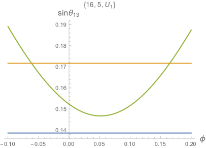
Figure 1: Case $el_{2}\left(16\right),\;el_{3}\left(5\right)$: The range of $\sin\theta_{13}$ as a function of the angle $\phi$ parametrizing the mixing  (50) of the degenerate subspace. The orange line defines the upper experimental bound and the blue the lower one on $\sin\theta_{13}$.

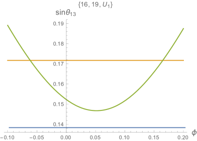
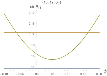
Figure 2: The acceptable range of $\sin\theta_{13}$ vs the angle $\varphi$ for the pair $el_{2}\left(16\right)~{}el_{3}\left(19\right)$ .

4.1.2 The pair $el_{2}\left(16\right)~{}el_{3}\left(19\right)$

The relevant matrix is

$$el_{3}\left(19\right)=\begin{bmatrix}r_{1}e^{\frac{2\pi i}{7}}&r_{2}e^{-\frac{5\pi i}{7}}&r_{3}e^{-\frac{5\pi i}{7}}\\ r_{2}e^{-\frac{3\pi i}{7}}&r_{3}e^{\frac{4\pi i}{7}}&r_{1}e^{\frac{4\pi i}{7}}\\ r_{3}e^{\frac{\pi i}{7}}&r_{1}e^{-\frac{6\pi i}{7}}&r_{2}e^{-\frac{6\pi i}{7}}\end{bmatrix}~{}.$$ (58)

The eigenvectors which correspond to the eigenvalues $1$, $e^{\frac{2\pi i}{3}}$, $e^{\frac{4\pi i}{3}}$ are

$$v_{3}\left[1\right] = N_{1}\{r_{2}\left(\eta^{-\frac{5}{2}}+\eta^{\frac{1}{2}}\right),\eta^{3}-r_{1}\eta^{4}+r_{3}\eta-r_{2},r_{1}\left(1+\eta\right)\}$$ (59)

$$v_{3}\left[2\right] = N_{2}\{r_{2}\left(\eta^{-\frac{5}{2}}+\eta^{\frac{17}{6}}\right),\eta^{\frac{23}{3}}-\eta^{\frac{7}{3}}\left(r_{2}+r_{1}\eta^{4}\right)+r_{3}\eta,r_{1}\left(\eta^{\frac{7}{3}}+\eta\right)\}$$ (60)

$$v_{3}\left[3\right] = N_{3}\left\{r_{2}\left(\eta^{-\frac{5}{2}}+\eta^{\frac{31}{6}}\right),\eta^{\frac{37}{3}}-\eta^{\frac{14}{3}}\left(r_{2}+r_{1}\eta^{4}\right)+r_{3}\eta,r_{1}\left(\eta^{\frac{14}{3}}+\eta\right)\right\}$$ (61)

where $N_{1}$ $N_{2}$ and $N_{3}$ are normalization factors. We find that a mixing matrix compatible with data occurs only for the two combinations

$$U_{1} = \begin{bmatrix}v_{3}\left[2\right],&v_{3}\left[1\right],&v_{3}\left[3\right]\end{bmatrix}^{\dagger}\cdot\begin{bmatrix}\tilde{v}_{2}\left[3\right],&v_{2}\left[1\right],&\tilde{v}_{2}\left[2\right]\end{bmatrix}$$ (62)

$$U_{2} = \begin{bmatrix}v_{3}\left[2\right],&v_{3}\left[3\right],&v_{3}\left[1\right]\end{bmatrix}^{\dagger}\cdot\begin{bmatrix}\tilde{v}_{2}\left[3\right],&v_{2}\left[1\right],&\tilde{v}_{2}\left[2\right]\end{bmatrix}~{}\cdot$$ (63)

In this case also, we find that the modulus of the second column elements for both matrices $U_{1}$and $U_{2}$ is $1/\sqrt{3}$. This is due to the fact that

$$\left\|v_{3}\left[1\right]^{\dagger}\cdot v_{2}\left[1\right]\right\|=\left\|v_{3}\left[2\right]^{\dagger}\cdot v_{2}\left[1\right]\right\|=\left\|v_{3}\left[3\right]^{\dagger}\cdot v_{2}\left[1\right]\right\|=\frac{1}{\sqrt{3}}$$ (64)

only for the given value of $s$ as in the previous case. For the pair $el_{2}\left(16\right)$ and $el_{3}\left(19\right)$ the mixing matrices for $\varphi=0$ are given by

$$U_{1}=\begin{bmatrix}0.80217e^{-1.82071i}&0.57735e^{-0.868576i}&0.152283e^{-3.1252i}\\ 0.36647e^{2.60604i}&0.57735e^{0.0831114i}&0.729634e^{-0.0791203i}\\ 0.471405e^{-3.09347i}&0.57735e^{1.25755i}&0.666667e^{-2.24541i}\end{bmatrix}$$

$$U_{2}=\begin{bmatrix}0.80217e^{-1.82071i}&0.57735e^{-0.868576i}&0.152283e^{-3.1252i}\\ 0.471405e^{-3.09347i}&0.57735e^{1.25755i}&0.666667e^{-2.24541i}\\ 0.36647e^{2.60604i}&0.57735e^{0.0831114i}&0.729634e^{-0.0791203i}\end{bmatrix}~{}\cdot$$

Again, making use of the degenerate subspace we can find the range of $\varphi$ values in accordance with the experimental findings. For the two examples above the range of $\varphi$ compatible with the experiment is between $[-0.0196,0.123]$ and is plotted in figure 2.

4.1.3 The pair $el_{2}\left(10\right)$, $el_{7}\left(23\right)$

We proceed now to an example which involves seventh-order elements of $PSL_{2}(7)$. We take the pair $el_{2}\left(10\right)$, $el_{7}\left(23\right)$ which is represented by the matrices

$$li_{2}\left(10\right)=\begin{bmatrix}r_{1}&-r_{2}&-r_{3}\\ -r_{2}&r_{3}&r_{1}\\ -r_{3}&r_{1}&r_{2}\end{bmatrix},\ li_{7}\left(23\right)=\begin{bmatrix}r_{1}e^{\frac{4\pi i}{7}}&r_{2}e^{\frac{\pi i}{7}}&r_{3}e^{-\frac{5\pi i}{7}}\\ r_{2}e^{-\frac{3\pi i}{7}}&r_{3}e^{-\frac{6\pi i}{7}}&r_{1}e^{\frac{2\pi i}{7}}\\ r_{3}e^{-\frac{3\pi i}{7}}&r_{1}e^{-\frac{6\pi i}{7}}&r_{2}e^{\frac{2\pi i}{7}}\end{bmatrix}~{}\cdot$$

The eigenvectors of $li_{2}\left(10\right)$ are

$$v_{2}\left[1\right]=\begin{bmatrix}\sqrt{\frac{2}{3}-s^{2}}\\ \frac{\sqrt{3}}{2}s+\frac{1}{2}\sqrt{\frac{2}{3}-s^{2}}\\ -\frac{\sqrt{3}}{2}s+\frac{1}{2}\sqrt{\frac{2}{3}-s^{2}}\end{bmatrix},\,\ v_{2}\left[2\right]=\frac{1}{\sqrt{3}}\begin{bmatrix}-1\\ 1\\ 1\end{bmatrix},\,\ v_{2}\left[3\right]=\begin{bmatrix}s\\ \frac{1}{2}s-\frac{\sqrt{3}}{2}\sqrt{\frac{2}{3}-s^{2}}\\ \frac{1}{2}s+\frac{\sqrt{3}}{2}\sqrt{\frac{2}{3}-s^{2}}\end{bmatrix}$$

corresponding to the eigenvalues $1$,$-1$, $-1$ repectively. Here $s$ is given by

$$s=\sqrt{\frac{2}{3}}\frac{\left(2+3r_{3}\right)}{\sqrt{3\left(1+r_{1}-r_{2}\right)^{2}+\left(2+3r_{3}\right)^{2}}}\approx 0.732\cdot$$ (65)

The normalized eigenvectors of $li_{7}\left(23\right)$ are given by

$$v_{7}\left[1\right]=\begin{bmatrix}r_{3}e^{\frac{4\pi i}{7}}\\ r_{1}e^{-\frac{5\pi i}{7}}\\ r_{2}e^{\frac{5\pi i}{7}}\end{bmatrix},\,v_{7}\left[2\right]=\begin{bmatrix}r_{2}e^{\frac{6\pi i}{7}}\\ r_{3}e^{-\frac{3\pi i}{7}}\\ -r_{1}\end{bmatrix},\,v_{7}\left[3\right]=\begin{bmatrix}-r_{1}\\ r_{2}e^{-\frac{2\pi i}{7}}\\ r_{3}e^{-\frac{6\pi i}{7}}\end{bmatrix}$$

and correspond to the eigenvalues $e^{\frac{6\pi i}{7}}$, $e^{\frac{10\pi i}{7}}$, $e^{\frac{12\pi i}{7}}$respectively. It turns out that the diagonalizing matrices of all order seven elements for some unclear reason can be written as latin square matrices which, however, do not constitute elements of the group. The mixing matrices compatible with data are

$$U_{1}=\begin{bmatrix}v_{7}\left[1\right]^{\dagger},&v_{7}[2]^{\dagger},&v_{7}\left[3\right]^{\dagger}\end{bmatrix}\cdot\begin{bmatrix}v_{2}\left[1\right],&\widetilde{v}_{2}\left[3\right],&\widetilde{v}_{2}\left[2\right]\end{bmatrix}$$ (66)

$$U_{2}=\begin{bmatrix}v_{7}\left[1\right]^{\dagger},&v_{7}[3]^{\dagger},&v_{7}\left[2\right]^{\dagger}\end{bmatrix}\cdot\begin{bmatrix}v_{2}\left[1\right],&\widetilde{v}_{2}\left[3\right],&\widetilde{v}_{2}\left[2\right]\end{bmatrix}~{}\cdot$$ (67)

Note that for $\varphi=0$ the mixing matrices are completely out. However, for $\phi=\frac{2\pi}{7}$ we get

$$U_{1}=\begin{bmatrix}0.814857e^{-\frac{3\pi i}{7}}&0.558406e^{\frac{\pi i}{14}}&0.15532e^{\frac{\pi i}{14}}\\ 0.362646e^{\frac{4\pi i}{7}}&0.700416e^{\frac{\pi i}{14}}&0.614741e^{-\frac{13\pi i}{14}}\\ 0.452212e^{-\frac{3\pi i}{7}}&0.444523e^{-\frac{13\pi i}{14}}&0.773242e^{--\frac{13\pi i}{14}}\end{bmatrix}$$

$$U_{2}=\begin{bmatrix}0.814857e^{-\frac{3\pi i}{7}}&0.558406e^{\frac{\pi i}{14}}&0.15532e^{\frac{\pi i}{14}}\\ 0.452212e^{-\frac{3\pi i}{7}}&0.444523e^{-\frac{13\pi i}{14}}&0.773242e^{--\frac{13\pi i}{14}}\\ 0.362646e^{\frac{4\pi i}{7}}&0.700416e^{\frac{\pi i}{14}}&0.614741e^{-\frac{13\pi i}{14}}\end{bmatrix}~{}.$$ (68)

The range of $\delta\varphi\equiv\varphi-\frac{2\pi}{7}$ that falls within the experimental bounds is very narrow, and is given by

$$-0.0028<\delta\varphi<+0.03$$ (69)

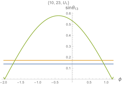
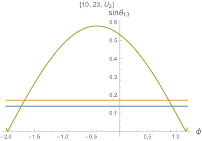
Figure 3: Plots show the experimentally compatible range of $\sin\theta_{13}$ as function of $\varphi$, for example 3 involving $PSL_{2}(7)$ elements of order 7. Orange and blue lines define the experimental bounds.

5 Summary and Conclusions

The last couple of decades, a substantial amount of research in physics beyond the Standard Model has been devoted to interpret the lepton mixing matrix, and in particular, the neutrino data. A rather established approach to this task is to postulate invariance of the Yukawa lagrangian under some suitable finite group. Remarkably, such symmetries appear naturally in a wide class of extensions of the Standard Model emerging in the framework of String and F-theory constructions. Given these facts and the continuing interest on these issues as well as the considerably wide applications of the discrete groups in phenomenological models, in this article, we focused our investigations on the projective linear group $PSL_{2}(7)$. This group is a simple discrete subgroup of $SU(3)$, and the largest one possessing three-dimensional unitary representations. Therefore it is a suitable candidate for a discrete flavor symmetry of the effective theory. However, despite its interesting features, its implications in low energy phenomenology have not been widely explored, partially because of the apparent complicated structure of the representations of its elements.

In this work we generate viable textures of charged-leptons neutrino mixing matrices by assuming that both types of matrices commute with some element of the $PSL_{2}(7)$ group. A tedious calculation reveals that the basic hypothesis is correct and it is valid for a number of group elements which are given in the context. It turns out that the neutrino mass matrix can only commute with order $2$ group elements while the charged leptons mass matrix can commute with both order $3$ and order $7$ elements. The results indicate there are only two types of matrices for the $\left(el_{3},el_{2}\right)$ combinations and also only two for the $\left(el_{7},el_{2}\right)$ combination. The eigenvector degeneracy of the $el_{2}$ elements (parametrized by a single parameter, the angle $\varphi$) may change somehow the values of the mixing angles. It appears though that the allowed values of the free parameter $\varphi$ are very strongly centered around a fixed value which is $\varphi=0$ for the $\left(el_{3},el_{2}\right)$ combination and $\varphi=\frac{2\pi}{7}$ for the $\left(el_{7},el_{2}\right)$. The value $\varphi=0$ suggests that nature prefers the eigenvector $\frac{1}{\sqrt{3}}\left(-1,\,1,\,1\right)$, which is independent of the values $\rho_{1},\rho_{2},\rho_{3}$ which characterize the group $PSL_{2}\left(7\right)$. In the more general case, this eigenvector is replaced by $\frac{1}{\sqrt{3}}{\left(e^{ic_{3}},e^{i\left(c_{3}-c_{2}\right)},1\right)}$ which is again independent of the values $\rho_{1},\rho_{2},\rho_{3}$ and the results obtained are similar to those presented here. Note that the algebra of the pairs $\left(el_{3},el_{2}\right)$ generate various $A_{4}$ subgroups of  $PSL_{2}\left(7\right)$. Probably this the reason for the appearance of the resulting mixing matrix as a generalization of the tri-bi-maximal mixing [16], i.e. the moduli of the middle column elements are equal to $\frac{1}{\sqrt{3}}$ a phenomenon which is known to be connected with an $A_{4}$ symmetry. Here, this simplification occurs non trivially because the form of the elements is very complicated. As for the $\left(el_{7},el_{2}\right)$ pairs, no $PSL_{2}\left(7\right)$ subgroup is generated a fact that leaves more space to the middle column elements to arrange themselves. Note that the allowed values of $\varphi$ are centered around the central value $\varphi=\frac{2\pi}{7}$ which is the phase associated with the basic seventh root of unity $e^{i\frac{2\pi}{7}}$.

Acknowledgement. NDV would like to thank Theory Division at CERN, for kind hospitality during the final stages of this work.

Appendix A Appendix

The following tables depict the correspondence between the $PSL_{2}\left(7\right)$ elements as calculated and enumerated by $GAP$ and their corresponding distribution among conjugacy classes used in the text.

• Character $-1$

  $$el_{2}$$

                

• Character $0$

  $$el_{3}$$

• Character $+1$

  $$el_{4}$$

      

• Character $-\frac{1}{2}-i\frac{\sqrt{7}}{2}$

  $$el_{7}$$

          

Appendix B
The general eigenvectors of the matrix $M$.

Given $\rho$ the three distinct eigenvalues of the matrix $M$ , the non-normalized eigenvectors are given by the expression

$$v=\left(e^{ic_{3}}r_{2}\left(1+\rho~{}e^{i\left(c_{1}+c_{5}\right)}\right),\,e^{i\left(c_{3}-c_{2}\right)}\left[\rho^{2}e^{i\left(c_{1}+c_{5}\right)}-\rho\left(r_{2}+r_{1}e^{i\left(2c_{1}+c_{5}\right)}\right)\right]+r_{3}e^{ic_{1}},\,r_{1}\left(\rho+e^{ic_{1}}\right)\right)\cdot$$

When normalized, while the $el_{2}$ and $el_{3}$ elements do not produce anything worth mentioning the $el_{7}$ eigenvectors produce diagonalizing matrices which are latin squares. All the phases can be exactly calculated however, the trace of the resulting matrix to the best of our knowledge does not correspond to a known group character so this tantalizing result must remain a curiosity for the time being.

References

[1]
G. Altarelli and F. Feruglio,
“Discrete Flavor Symmetries and Models of Neutrino Mixing,”
Rev. Mod. Phys. 82 (2010) 2701
doi:10.1103/RevModPhys.82.2701
[arXiv:1002.0211 [hep-ph]].
[2]
H. Ishimori, T. Kobayashi, H. Ohki, Y. Shimizu, H. Okada and M. Tanimoto,
“Non-Abelian Discrete Symmetries in Particle Physics,”
Prog. Theor. Phys. Suppl. 183 (2010) 1
doi:10.1143/PTPS.183.1
[arXiv:1003.3552 [hep-th]].
[3]
S. F. King and C. Luhn,
“Neutrino Mass and Mixing with Discrete Symmetry,”
Rept. Prog. Phys. 76 (2013) 056201
doi:10.1088/0034-4885/76/5/056201
[arXiv:1301.1340 [hep-ph]].
[4]
A. Karozas, S. F. King, G. K. Leontaris and A. Meadowcroft,
“Discrete Family Symmetry from F-Theory GUTs,”
JHEP 1409 (2014) 107
doi:10.1007/JHEP09(2014)107
[arXiv:1406.6290 [hep-ph]].
[5]
S. Tanaka,
“Construction and classification of irreducible representations of special
linear group of the second order over a finite field”,
Osaka J. Math. Volume 4, Number 1 (1967), 65-84.
[6]
J. E. Humphreys,
“ Representations of SL(2,p)”, Amer. Math. Monthly 82(1975)21.
[7]
C. Luhn, S. Nasri and P. Ramond,
“Simple Finite Non-Abelian Flavor Groups,”
J. Math. Phys. 48 (2007) 123519
doi:10.1063/1.2823978
[arXiv:0709.1447 [hep-th]].
[8]
S. F. King and C. Luhn,
“A Supersymmetric Grand Unified Theory of Flavour with PSL(2)(7) x SO(10),”
Nucl. Phys. B 832 (2010) 414
doi:10.1016/j.nuclphysb.2010.02.019
[arXiv:0912.1344 [hep-ph]].
[9]
R. de Adelhart Toorop, F. Feruglio and C. Hagedorn,
“Finite Modular Groups and Lepton Mixing,”
Nucl. Phys. B 858 (2012) 437
doi:10.1016/j.nuclphysb.2012.01.017
[arXiv:1112.1340 [hep-ph]].
[10]
E. G. Floratos and G. K. Leontaris,
“Discrete Flavour Symmetries from the Heisenberg Group,”
Phys. Lett. B 755, 155 (2016)
doi:10.1016/j.physletb.2016.02.007
[arXiv:1511.01875 [hep-th]].
[11]
C. Beasley, J. J. Heckman and C. Vafa,
“GUTs and Exceptional Branes in F-theory - II: Experimental Predictions,”
JHEP 0901 (2009) 059
doi:10.1088/1126-6708/2009/01/059
[arXiv:0806.0102 [hep-th]].
[12]
R. Balian and C. Itzykson,
“Observations sur la mecanique quantique finie”,
C. R. Acad. Sc. Paris 303, serie 1, No. 16, (1986) 773-778.
[13]
G. G. Athanasiu and E. G. Floratos,
“Coherent states in finite quantum mechanics,”
Nucl. Phys. B 425 (1994) 343.