Restoration of dimensional reduction in the random–field Ising model at five dimensions

Abstract

The random-field Ising model is one of the few disordered systems where the perturbative renormalization group can be carried out to all orders of perturbation theory. This analysis predicts dimensional reduction, i.e., that the critical properties of the random-field Ising model in $D$ dimensions are identical to those of the pure Ising ferromagnet in $D-2$ dimensions. It is well known that dimensional reduction is not true in three dimensions, thus invalidating the perturbative renormalization group prediction. Here, we report high-precision numerical simulations of the 5D random-field Ising model at zero temperature. We illustrate universality by comparing different probability distributions for the random fields. We compute all the relevant critical exponents (including the critical slowing down exponent for the ground-state finding algorithm), as well as several other renormalization-group invariants. The estimated values of the critical exponents of the 5D random-field Ising model are statistically compatible to those of the pure 3D Ising ferromagnet. These results support the restoration of dimensional reduction at $D=5$. We thus conclude that the failure of the perturbative renormalization group is a low-dimensional phenomenon. We close our contribution by comparing universal quantities for the random-field problem at dimensions $3\leq D<6$ to their values in the pure Ising model at $D-2$ dimensions and we provide a clear verification of the Rushbrooke equality at all studied dimensions.

I Introduction

In the study of phase transitions under the presence of quenched disorder Parisi (1994), the straightforward application of field theoretic methods and the renormalization group (RG) is not possible because the disorder breaks the translation symmetry of the Hamiltonian. The standard procedure is then to average over disorder using the replica method Edwards and Anderson (1975). One starts with $n$ noninteracting copies of the system (replicas) and averages over the disorder distribution. This produces an effective Hamiltonian with $n$ interacting fields which is translation invariant and enables the use of the RG. In the end, the $n\to 0$ limit has to be taken.

The replica method is mathematically unorthodox. Its combination with the perturbative renormalization group (PRG) has been shown to produce incorrect results in 3D systems. A warning example is provided by the random-field Ising model (RFIM) where the combination of the replica method with the PRG predicts dimensional reduction Young (1977); Parisi and Sourlas (1979) (see below), which does not hold neither in three Bricmont and Kupiainen (1987) nor in four dimensions Fytas et al. (2016a). On the other hand, the replica method has been proven correct in the case of branched polymers, as well as for the highly non trivial problem of mean-field spin glasses Talagrand (2006); Panchenko (2013). Mean field and the replica method are believed to be correct at infinite dimensions.

The RFIM is probably the best studied problem in this context, both for its simplicity and physical relevance. In fact, the RFIM is one of the two well-known disordered systems (the other one refers to the case of branched polymers) that can be analyzed to all orders of perturbation theory, thanks to the existence of a hidden supersymmetry Parisi and Sourlas (1979). The PRG analysis predicts the phenomenon of dimensional reduction: The critical properties of the RFIM in $D$ dimensions should be the same as those of the pure Ising ferromagnet at $D-2$ dimensions. It is by now well established that this prediction is not true in three dimensions because the 3D RFIM orders Bricmont and Kupiainen (1987), while the 1D pure Ising ferromagnet does not.

One central problem is to understand the reason of the failure of the PRG. Since dimensional reduction is proven to all orders of perturbation theory, the reasons of its failure must be non perturbative. Parisi and Sourlas argue that in the case of the RFIM in three dimensions the interaction between replicas is attractive and leads to the formation of bound states between replicas Parisi and Sourlas (2002). The presence of bound states is a non perturbative phenomenon. The mass of the bound state provides a new length scale which is not taken into account in the traditional PRG analysis. The authors of Ref. Parisi and Sourlas (2002) also provide a physical interpretation: These bound states indicate that the correlation length is not self-averaging Parisi and Sourlas (2002).

Figure 1: Connected correlation length in units of the system size $L$ vs. $\sigma$ for the Gaussian 5D RFIM (we show data only for some characteristic $L$ values for clarity’ sake). Due to scale invariance, all curves should cross at the critical point $\sigma_{\mathrm{c}}$. Yet, small systems deviate from the large-$L$ scale-invariant behavior.

Although the finding of Parisi and Sourlas is numerical, we have more indications for the presence of bound states. Brézin and De Dominicis have also noticed that the forces between replicas are attractive and that the Bethe-Salpeter kernel, for a pair of replicas of different indices, develops an instability for $D\leq 6$ hinting towards the existence of bound states among replicas Brézin and De Dominicis (1998, 2001). Similar conclusions were reached by Kardar and coworkers, who studied the problem of 2D interfaces Kardar and Zhang (1987); Kardar (1987); Medina et al. (1989); Medina and Kardar (1993). Indeed, using the Bethe ansatz method, these authors solved the replica Hamiltonian, thus finding that bound states form when the number of replicas is $n<1$. Bound states were also found in the case of the random Potts ferromagnet in two dimensions Parisi et al. (2004).

Identifying the existence (or lack thereof) of bound states as the crucial factor for the validity of the PRG immediately suggests that the space dimension should play a crucial role. In fact, we know from constructive field theory that in the formation of bound states there is a competition between the attractive interactions and the size of the available phase space. In two dimensions the phase space is small and any infinitesimal attraction is enough to form bound states Dimock and Eckmann (1976). The size of the phase space increases when the dimension of space gets larger. In higher dimensions the formation of bound states depends on the strength of the attractive forces. We expect that for high enough dimensions bound states will no longer exist, thus implying that the PRG prediction of dimensional reduction should eventually hold.

Figure 2: $\xi^{\mathrm{(con)}}/L$ (top) and $\eta^{\mathrm{(eff)}}$ (bottom) vs. $L^{-\omega}$. Lines correspond to the joint quadratic ($a_{3}=0$) fit (6) reported in Tab. 1 with $\omega=0.66$. The points at $L^{-\omega}=0$ mark our infinite volume extrapolation with their error bars.

The natural question to ask then is if there exists an intermediate dimension $D_{\mathrm{int}}$ below the upper critical dimension $D_{\rm u}=6$ Aharony (1978) such that the PRG and replicas are valid for dimensions $D>D_{\mathrm{int}}$ and false for $D<D_{\mathrm{int}}$. This $D_{\mathrm{int}}$ may depend on the physical system. Tarjus et al. using functional RG arguments concluded that such $D_{\mathrm{int}}$ exists for the RFIM and that it is close to $D=5$. In particular they found $D_{\mathrm{int}}\simeq 5.1$ Tissier and Tarjus (2011, 2012); Tarjus et al. (2013).

Here we report large-scale zero-temperature numerical simulations of the RFIM at five spatial dimensions. Our analysis benefits from recent advances in finite-size scaling and reweighting methods for disordered systems Fytas and Martín-Mayor (2013, 2016). By using two different random-field distribution we are able to show the universality of the critical exponents characterizing the transition. Our results are compatible with dimensional reduction being restored in five dimensions: We find that the critical exponents of the 5D RFIM are compatible to those of the pure 3D Ising ferromagnet up to our relatively small simulation errors, and in agreement to the suggestion by Tarjus et al. Tissier and Tarjus (2011, 2012); Tarjus et al. (2013).

The outline of the article is as follows: In Sec. II the model and methods employed are described shortly and in Sec. III our main results on the universality principle and the critical exponents of the 5D RFIM are presented. We conclude this article in Sec. IV by providing an overview of the model’s critical behavior in dimensions $3\leq D<D_{\rm u}$, which is compared to that of the pure Ising ferromagnet under the prism of dimensional reduction.

Figure 3: $\xi^{\mathrm{(dis)}}/L$ vs. $L^{-\omega}$. Lines correspond to a joint quadratic ($a_{3}=0$) fit (6) with $\omega=0.66$. The point at $L^{-\omega}=0$ marks our infinite volume extrapolation with its error bar.

II Model and Methods

The Hamiltonian of the RFIM is

$${\cal H}=-J\sum_{<xy>}S_{x}S_{y}-\sum_{x}h_{x}S_{x}\;,$$ (1)

with the spins $S_{x}=\pm 1$ on a hypercubic lattice in $D$ dimensions with nearest-neighbor ferromagnetic interactions and $h_{x}$ independent random magnetic fields with zero mean and variance $\sigma$. A given realization of the random fields $\{h_{x}\}$ is named a sample. Because the disorder is quenched, one first takes thermal mean values for a sample, denoted as $\langle\cdots\rangle$, and only then average over samples, which we indicate by an over-line (for instance, for the magnetization density $m=\sum_{x}S_{x}/L^{D}$ we consider first $\langle m\rangle$ and then $\overline{\langle m\rangle}$).

It is established that the relevant fixed point of the model lies at zero temperature Villain (1984); Bray and Moore (1985); Fisher and Huse (1986). Therefore, the only spin configuration that we shall consider in the present work is the ground state for each specific realization of the Hamiltonian (1) on a $D=5$ hypercubic lattice with periodic boundary conditions and energy units $J=1$. Our random fields $h_{x}$ follow either a Gaussian $({\mathcal{P}}_{G})$, or a Poissonian $({\mathcal{P}}_{P})$ distribution:

$${\mathcal{P}}_{G}(h,\sigma)={1\over\sqrt{2\pi\sigma^{2}}}e^{-{h^{2}\over 2\sigma^{2}}}\;,\ {\mathcal{P}}_{P}(h,\sigma)={1\over 2|\sigma|}e^{-{|h|\over\sigma}}\;,$$ (2)

where $-\infty<h<\infty$. As it is clear, for both distributions $\sigma$ is our single control parameter.

There are two relevant propagators for the RFIM, namely the connected, $C^{\mathrm{(con)}}$, and disconnected one $C^{\mathrm{(dis)}}$. At the critical point and for large $r$ ($r$ being the distance between $x$ and $y$) they decay as:

$$C^{\mathrm{(con)}}_{xy} \equiv \frac{\partial\overline{\langle S_{x}\rangle}}{\partial h_{y}}\ \sim\ \frac{1}{r^{D-2+\eta}}\,,$$ (3)

$$C^{\mathrm{(dis)}}_{xy} \equiv \overline{\langle S_{x}\rangle\langle S_{y}\rangle}\ \sim\ \frac{1}{r^{D-4+\bar{\eta}}}\,.$$ (4)

The above expressions define as well the two relevant anomalous dimensions, $\eta$ and $\bar{\eta}$. For each of these two propagators we shall consider the second-moment correlation lengths Amit and Martín-Mayor (2005), denoted as $\xi^{\mathrm{(con)}}$ and $\xi^{\mathrm{(dis)}}$, respectively. Hereafter, we shall indicate with the superscript “$\mathrm{con}$”, e.g. $\xi^{\mathrm{(con)}}$, quantities computed from the connected propagator. Similarly, the superscript “$\mathrm{dis}$”, e.g. $\xi^{\mathrm{(dis)}}$, will refer to the propagator $C^{\mathrm{(dis)}}$.

Figure 4: $U_{4}$ vs. $L^{-\omega}$. Lines correspond to a joint cubic fit (6) with $\omega=0.66$. The point at $L^{-\omega}=0$ marks our infinite volume extrapolation with its error bar.

We simulated lattice sizes from $L_{\rm min}=4$ to $L_{\rm max}=28$. For each $L$ and $\sigma$ value we computed ground states for $10^{7}$ samples. For comparison: $5000$ samples of $L_{\rm max}=14$ were simulated in Ref. Ahrens and Hartmann (2011). Our simulations and analysis closely follow our previous work at $D=3$ and $4$ Fytas and Martín-Mayor (2013); Fytas et al. (2016a) (see Ref. Fytas and Martín-Mayor (2016) for full details). Thus, we just briefly recall here the fundamental aspects of our computation.

The algorithm used to generate the ground states of the system was the push-relabel algorithm of Tarjan and Goldberg Goldberg and Tarjan (1988). We prepared our own C version of the algorithm, involving a modification proposed by Middleton et al. Middleton (2001); Middleton and Fisher (2002); Middleton (2002) that removes the source and sink nodes, reducing memory usage and also clarifying the physical connection Middleton and Fisher (2002); Middleton (2002). Additionally, the computational efficiency of our algorithm has been increased via the use of periodic global updates Middleton and Fisher (2002); Middleton (2002).

From simulations at a given $\sigma$, we computed $\sigma$-derivatives and extrapolated to neighboring $\sigma$ values by means of a reweighting method Fytas and Martín-Mayor (2013, 2016).

We also computed the corresponding susceptibilities $\chi^{\mathrm{(con)}}$ and $\chi^{\mathrm{(dis)}}$, as well as the dimensionless Binder ratio $U_{4}=\overline{\langle m^{4}\rangle}/\overline{\langle m^{2}\rangle}^{2}$ and the ratio $U_{22}=\chi^{\mathrm{(dis)}}/[\chi^{\mathrm{(con)}}]^{2}$ that gives a direct access to the difference of the anomalous dimensions $2\eta-\bar{\eta}$ Fytas and Martín-Mayor (2013, 2016).

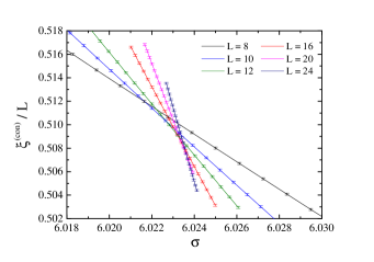
We followed the quotients-method approach to finite-size scaling Amit and Martín-Mayor (2005); Nightingale (1976); Ballesteros et al. (1996). In this method one considers dimensionless quantities $g(\sigma,L)$ that, barring correction to scaling, are $L$-independent at the critical point. We consider three such $g$, namely $\xi^{\mathrm{(con)}}/L$, $\xi^{\mathrm{(dis)}}/L$, and $U_{4}$. Given a dimensionless quantity $g$, we consider a pair of lattices sizes $L$ and $2L$ and determine the crossing $\sigma_{\mathrm{c},L}$, where $g(\sigma_{\mathrm{c},L},L)=g(\sigma_{\mathrm{c},L},2L)$, see Fig. 1. For each random-field distribution we computed three such $\sigma_{\mathrm{c},L}$, a first for $\xi^{\mathrm{(con)}}/L$, another for $\xi^{\mathrm{(dis)}}/L$, and a third for $U_{4}$. Crossings approach the critical point $\sigma_{\mathrm{c}}$ as $\sigma_{\mathrm{c}}-\sigma_{\mathrm{c},L}={\cal O}(L^{-(\omega+1/\nu)})$, with $\omega$ being the leading corrections-to-scaling exponent.

Dimensionful quantities $O$ scale with $\xi$ in the thermodynamic limit as $\xi^{x_{O}/\nu}$, where $x_{O}$ is the scaling dimension of $O$. At finite $L$, we consider the quotient $Q_{O,L}=O_{2L}/O_{L}$ at the crossing (for dimensionless magnitudes $g$, we write $g^{\mathrm{cross}}_{L}$ for either $g_{L}$ or $g_{2L}$, whichever shows less finite-size corrections)

$$Q_{O,L}^{\mathrm{cross}}=2^{x_{O}/\nu}+O(L^{-\omega})\;\;;\;\;g^{\mathrm{cross}}_{L}=g^{\ast}+O(L^{-\omega})\,.$$ (5)

$Q_{O}^{\mathrm{cross}}$ (or $g^{\mathrm{cross}}_{L}$) can be evaluated at the crossings of $\xi^{\mathrm{(con)}}/L$, $\xi^{\mathrm{(dis)}}/L$, and $U_{4}$. The three choices differ only in the scaling corrections, an opportunity we shall use. The RG tells us that $x_{O}$, $g^{\ast}$, $\omega$, and $\nu$, are universal. We shall compute the critical exponents using Eq. (5) with the following dimensionful quantities: $\sigma$-derivatives [$x_{D_{\sigma}\xi^{\mathrm{(con)}}}=x_{D_{\sigma}\xi^{\mathrm{(dis)}}}=1+\nu$], susceptibilities [$x_{\chi^{\mathrm{(con)}}}=\nu(2-\eta)$ and $x_{\chi^{\mathrm{(dis)}}}=\nu(4-\bar{\eta})$] and the ratio $U_{22}$ [$x_{U_{22}}=\nu(2\eta-\bar{\eta})$].

Figure 5: Effective anomalous dimension difference $(2\eta-\bar{\eta})^{\rm(eff)}$ vs. $L^{-\omega}$. Lines correspond to a joint leading-term ($a_{2}=a_{3}=0$) fit (6) with $\omega=0.66$. The point at $L^{-\omega}=0$ marks our infinite volume extrapolation with its error bar.

As we applied the quotients method at the crossings of $\xi^{\rm(con)}/L$, $\xi^{\rm(dis)}/L$, and $U_{4}$, typically the data sets of our simulations were tripled for each pair of system sizes used. Note also, that throughout the manuscript we shall use the notation $\rm{Z}^{\rm(x)}$, where Z denotes the distribution - G for Gaussian and P for Poissonian - and the superscript x the crossing type considered - (con), (dis), or ($U_{4}$) - for $\xi^{\rm(con)}/L$, $\xi^{\rm(dis)}/L$, and $U_{4}$, respectively.

Since the size evolution can be non-monotonic as will be also seen below in the relevant figures, and given that our accuracy is enough to resolve sub-leading corrections to scaling, we take these into account in an effective way: Let $X_{L}$ be either $g^{\mathrm{cross}}_{L}$ or the effective scaling dimension $x^{\mathrm{(eff)}}_{O}/\nu=\log Q_{O}^{\mathrm{cross}}(L)/\log 2$, recall Eq. (5). We consider the following generalized fitting functions

$$X_{L} = X^{\ast}+a_{1}L^{-\omega}+a_{2}L^{-2\omega}+a_{3}L^{-3\omega}\;,$$ (6)

$$\sigma_{\mathrm{c},L} = \sigma_{c}+b_{1}L^{-(\omega+\frac{1}{\nu})}+b_{2}L^{-(2\omega+\frac{1}{\nu})}\;,$$ (7)

where $a_{k}$, with $k=1,2,3$, and $b_{l}$, with $l=1,2$, are scaling amplitudes.

For the fitting procedure discussed below we restricted ourselves to data with $L\geq L_{\mathrm{min}}$. As usual, to determine an acceptable $L_{\mathrm{min}}$ we employed the standard $\chi^{2}$-test for goodness of fit, where $\chi^{2}$ was computed using the complete covariance matrix. Specifically, the $p$-value of our $\chi^{2}$-test – also known as $Q$, see e.g. Ref. Press et al. (1992) – is the probability of finding a $\chi^{2}$ value which is even larger than the one actually found from our data. Recall that this probability is computed by assuming: (i) Gaussian statistics and (ii) the correctness of the fit’s functional form. We consider a fit as being fair only if $10\%<Q<90\%$. Generally speaking, we observed that, once a fair fit is found, increasing $L_{\mathrm{min}}$ doubles (or worsens) the errors in the extrapolation to $L=\infty$. However, increasing the order of $L^{-\omega}$ in fits to Eq. (6) is even more detrimental to the error in the extrapolation $X^{*}$. Therefore, we first decide the order of the fit. Starting from linear in $L^{-\omega}$ corrections to scaling, we increase $L_{\mathrm{min}}$ from $L_{\mathrm{min}}=4$ and check if the resulting fit is acceptable (i.e., whether or not the $p$-value satisfies our constraint $10\%<Q<90\%$). If the fit’s quality is not acceptable, we increase $L_{\mathrm{min}}$ to the larger available $L$ and try to fit again. In the case where we exhaust the number of available system sizes without finding a fair fit, we move on to quadratic scaling corrections. If an $L_{\mathrm{min}}$ yielding an acceptable fit cannot be identified, then we consider corrections to scaling of order $L^{-3\omega}$. As a rule, we keep the lowest order for which an acceptable $L_{\mathrm{min}}$ can be found. Having decided the order of $L^{-\omega}$ in Eq. (6), we also keep the smallest possible $L_{\mathrm{min}}$.

III Evidence for Dimensional Reduction at $D=5$

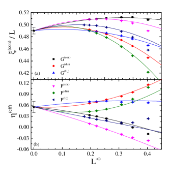
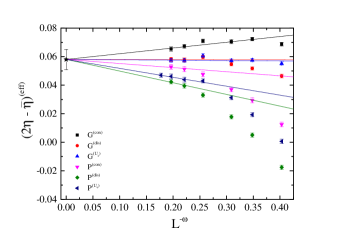
The procedure we follow is standard by now Ballesteros et al. (1998). The first step is the estimation of the corrections-to-scaling exponent $\omega$. Take, for instance, $\xi^{\mathrm{(con)}}/L$. For each pair of sizes $(L,2L)$ we have six estimators: Three crossing points, $\xi^{\mathrm{(con)}}/L$, $\xi^{\mathrm{(dis)}}/L$, and $U_{4}$, and two disorder distributions, Gaussian and Poissonian. Rather than six independent polynomial fits to some degree of Eq. (6), we perform a single joint fit: We minimize the combined $\chi^{2}$ goodness-of-fit, by imposing that the extrapolation to $L=\infty$ (depicted as a black star at the origin of the horizontal axis for all the figures below), $(\xi^{\mathrm{(con)}}/L)^{\ast}$, as well as exponent $\omega$ are common for all six estimators (only the scaling amplitudes differ). We judge from the final $\chi^{2}$ value whether or not the fit is fair.

Figure 6: Effective critical exponent $\nu^{\rm(eff)}$ vs. $L^{-\omega}$. Lines correspond to a joint leading-term ($a_{2}=a_{3}=0$) fit (6) with $\omega=0.66$. The point at $L^{-\omega}=0$ marks our infinite volume extrapolation with its error bar.

Figure 7: Crossing points $\sigma_{\mathrm{c},L}$ for Gaussian (main panel) and Poissonian (inset) random fields. Lines are fits to Eq. (7), constrained to yield a common extrapolation at $L=\infty$.

Furthermore, one can perform joint fits for several magnitudes, say $\xi^{\mathrm{(con)}}/L$ and $\eta$. Of course, the extrapolation to $L=\infty$ is different for each magnitude, but a common $\omega$ is imposed. However, when we increase the number of magnitudes, the covariance matrix becomes close to singular due to data correlation and the fit unstable. Therefore, we limit ourselves to $\xi^{\mathrm{(con)}}/L$ and $\eta$, see Fig. 2. We obtain a fair fit by considering pairs $(L,2L)$ with $L\geq L_{\mathrm{min}}=8$, see Tab. 1. Indeed there are not many other available choices of pairs of observables to be considered in a joint fit, unless one is willing to consider third-order corrections to scaling (see for instance the data for $U_{4}$ in Fig. 4). Given that our lattice sizes range from $L=4$ up to $L=28$, we prefer to keep the order of the scaling corrections as low as possible in the computation of $\omega$.

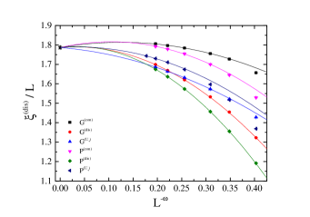
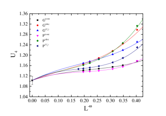
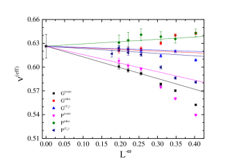
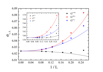
The rest of the quantities of interest are individually extrapolated, following the same procedure, but now fixing $\omega=0.66$, the value obtained in the joint fit of Fig. 2. For the extrapolation of the dimensionless quantities $\xi^{\mathrm{(dis)}}/L$ and $U_{4}$ we refer the reader to Figs. 3 and 4. The extrapolation of the difference $2\eta-\bar{\eta}$ and the critical exponent $\nu$ of the correlation length are illustrated in Figs. 5 and 6, respectively. In particular, in Fig. 5 we show $\log U_{22}/\log 2$ which is a direct measurement of the difference $2\eta-\bar{\eta}$ and in Fig. 6 the effective values of $\nu$ estimated as the derivatives of $\xi^{\rm(dis)}$ for all data sets at hand (the statistical errors of the other $\nu$-estimators were rather large and therefore omitted from the fits). Finally, in Fig. 7 the critical fields for both the Gaussian (main panel) and Poissonian (inset) 5D RFIM are estimated via a joint fit of the form (7).

The final values we quote for all our observables are summarized in Tab. 1. In fact, the extrapolations in Tab. 1 have two error bars. The first error, obtained from the corresponding joint fit to Eqs. (6) and (7) is of statistical origin. The second error is systematic and takes into account how much the extrapolation to $L=\infty$ changes within the range $0.53<\omega<0.81$.

Table 1: Summary of results for the 5D RFIM. The first column is the outcome of a fit to Eq. (6) (critical points $\sigma_{\mathrm{c}}$ were obtained from Eq. (7), respectively). The second column is the standard figure of merit, $\chi^{2}/{\rm DOF}$, where DOF denotes the number of degrees of freedom. The third column gives the minimum system size used in the fits and the last column the degree of the polynomial in $L^{-\omega}$. The first set of rows reports a joint fit for $\xi^{\mathrm{(con)}}/L$, $\eta$, and $\omega$. The remaining quantities were individually extrapolated to $L=\infty$. The error induced by the uncertainty in $\omega$ is given as a second error estimate in the square brackets.

Extrapolation to $L\rightarrow\infty$		$\chi^{2}/{\rm DOF}$	$L_{\rm min}$	order in $L^{-\omega}$
$\xi^{\rm(con)}/L$ =	$0.4901(55)$	$11.3/10$	8	second
$\eta$ =	$0.055(15)$
$\omega$ =	$0.66(+15/-13)$
$\xi^{\rm(dis)}/L$ =	$1.787(8)[+30/-82]$	$5.3/9$	6	second
$U_{4}$ =	$1.103(16)[+18/-43]$	$1.9/6$	6	third
$2\eta-\bar{\eta}$ =	$0.058(7)[+1/-2]$	$3.8/6$	10	first
$\nu$ =	$0.626(15)[+2/-3]$	$8.3/6$	10	first
$\sigma_{\rm c}({\rm G})$ =	$6.02395(7)[+2/-7]$	$0.1/2$	8	second
$\sigma_{\rm c}({\rm P})$ =	$5.59038(16)[+9/-13]$	$2.7/3$	8	second

Figure 8: Effective critical slowing down exponent $z^{\rm(eff)}$ of the push-relabel algorithm vs. $L^{-\omega}$. The point at $L^{-\omega}=0$ marks our infinite volume extrapolation with its error bar.

Table 2: Fitting tests and results after accepting the null hypothesis of restoration of dimensional reduction at $D=5$. The first two columns refer to the observable and the $L\rightarrow\infty$ extrapolation, respectively. The third column gives the standard figure of merit $\chi^{2}/{\rm DOF}$. The fourth column is the $p$-value of our $\chi^{2}$ tests (namely, the probability of $\chi^{2}$ to be even larger than what we actually found, should the null hypothesis hold). Finally, the fifth and sixth columns give the minimum size used in the fits and the degree of the polynomial in $L^{-\omega}$. The first two row-sets of results refer to the joint fit (6), by fixing in the first case $\omega$ to the Ising value and in the second case both $\omega$ and the extrapolated value of $\eta$ to their Ising values. The following rows refer to either universal ratios, critical exponents, or critical points. For the case of universal ratios we have fixed $\omega$ to the Ising value, whereas for the cases of $2\eta-\bar{\eta}$ and $\nu$ we ave fixed both $\omega$ to the Ising value but also their extrapolation values to $2\eta-\bar{\eta}=\eta=0.036298$ and $\nu=0.629971$. Finally, for the case of critical points we have fixed both $\omega$ and $\nu$ to the Ising values in the fits. The values of $\omega$, $\eta$, and $\nu$ of the 3D Ising universality class have been taken from Ref. Kos et al. (2016).

Observable	Extrapolation to $L\rightarrow\infty$	$\chi^{2}/{\rm DOF}$	$p$-value	$L_{\rm min}$	order in $L^{-\omega}$
$\xi^{\rm(con)}/L$	$0.4972(+16/-35)$
$\eta$	$0.0453(+19/-44)$	$13.37/11$	$27\%$	8	second
$\omega$	$0.82966$ (fixed)
$\eta$	$0.036298$ (fixed)	$15.82/12$	$20\%$	8	second
$\omega$	$0.82966$ (fixed)
$\xi^{\rm(dis)}/L$	$1.8184(52)$	$13.08/9$	$16\%$	6	second
$U_{4}$	$1.123(8)$	$2.76/6$	$84\%$	6	third
$2\eta-\bar{\eta}$	$0.036298$ (fixed)	$4.15/7$	$76\%$	8	second
$\nu$	$0.629971$ (fixed)	$3.43/7$	$84\%$	8	second
$\sigma_{\rm c}({\rm G})$	$6.02393(18)$	$0.95/2$	$62\%$	8	second
$\sigma_{\rm c}({\rm P})$	$5.59028(13)$	$2.01/3$	$57\%$	8	second

At this point several comments are in order:

• For dimensionless quantities we needed a second-order polynomial in $L^{-\omega}$ to extrapolate our data, apart from $U_{4}$ where a cubic term was necessary for the fit. On the other hand, leading-order corrections sufficed for a safe estimation of the critical exponent $\nu$ and the difference $2\eta-\bar{\eta}$.

• We are not aware of any other previous computation of the corrections-to-scaling exponent $\omega$ and of the dimensionless ratios $\xi^{\mathrm{(con)}}/L$, $\xi^{\mathrm{(dis)}}/L$, and $U_{4}$ in the 5D RFIM. As it was shown above in Figs. 2, 3, and 4, all of them are universal and together with the recently reported results of the 3D and 4D RFIM Fytas and Martín-Mayor (2013); Fytas et al. (2016a), they provide a complete picture of universality in terms of different field distributions in the random-field problem.

• Our values for the critical exponents $\eta$ and $\nu$ (including the corrections-to-scaling exponent $\omega$ and the difference $2\eta-\bar{\eta}$) are compatible within statistical accuracy to the values of the pure 3D Ising ferromagnet: $\eta=2\eta-\bar{\eta}=\bar{\eta}=0.036298(2)$, $\nu=0.629971(4)$, and $\omega=0.82966(9)$ Kos et al. (2016), thus indicating that within simulation errors, dimensional reduction gets restored at five dimensions. As it can be seen from the results of Tab. 1, a larger deviation among the computed exponents and those of the Ising universality appears in the anomalous dimensions. Of course, the computation of such small numbers is a harsh task.

• Notwithstanding, one would like to have a clear-cut answer to the following important question: Are the critical exponents of the 5D RFIM (even to our high accuracy) compatible to those of the 3D pure Ising ferromagnet? In order to answer quantitatively the question, we make the null-hypothesis of equality of the two universality classes. Indeed, in Tab. 2 we provide the figure of merit $\chi^{2}/\mathrm{DOF}$, as well as the corresponding $p$-values, for fits where the extrapolation to $L=\infty$ and the corrections-to-scaling $\omega$ were taken from the 3D pure Ising universality class. All fits, for which the extrapolation to $L=\infty$ is known for the 3D pure Ising ferromagnet, are denoted as (fixed) in Tab. 2. We remark that those 3D extrapolations are known to such a high-accuracy Kos et al. (2016), that we can regard them as virtually exact. As the reader can check in Tab. 2, for all the extrapolations assuming 3D pure Ising universality we could identify an appropriate $L_{\mathrm{min}}$ that makes the fit fair. So, the answer to the above question is that at least within our level of accuracy (which is set by the results shown in Tab. 1), the two universality classes of the 5D RFIM and the 3D pure Ising ferromagnet, cannot be distinguished.

• We note the discrepancy in the determination of the critical point for the Gaussian RFIM: Ref. Ahrens and Hartmann (2011) quotes $\sigma_{\rm c}(G)=6.0157(10)$. This difference is probably explained by the fact that in Ref. Ahrens and Hartmann (2011) corrections-to-scaling were not taken into account and that our statistics is much higher.

Table 3: Illustrative summary of results for the $D$-dimensional RFIM, where $D=3$, $4$, and $D=5$. In particular four row-sets of results are shown: critical exponents (first set), the verification of the Rushbrooke relation (second set), critical points (third set), and universal ratios and the corrections-to-scaling exponent $\omega$ (fourth set). For the case of the critical exponent $\alpha$ we show two estimates, one direct estimation Fytas and Martín-Mayor (2016); Fytas et al. (2016b) and another one based on the modified hyperscaling relation. Corresponding results of the 2D and 3D pure Ising ferromagnet are also included in the fifth and sixth columns for comparison. The last column contains mean-field (MF) results.

	3D RFIM Fytas and Martín-Mayor (2013, 2016)	4D RFIM Fytas et al. (2016a, b)	5D RFIM (current work)	2D IM McCoy and Wu (1973)	3D IM Kos et al. (2016)	MF
$\nu$	1.38(10)	0.8718(58)	0.626(15)	1	0.629971 (4)	1/2
$\eta$	0.5153(9)	0.1930(13)	0.055(15)	0.25	0.036298(2)	0
$\bar{\eta}$	1.028(2)	0.3538(35)	0.052(30)	0.25	0.036298(2)	0
$\Delta_{\eta,\bar{\eta}}=2\eta-\bar{\eta}$	0.0026(9)	0.0322(23)	0.058(7)	0.25	0.036298(2)	0
$\beta$	0.019(4)	0.154(2)	0.329(12)	0.125	0.326419(3)	1/2
$\gamma$	2.05(15)	1.575(11)	1.217(31)	1.875	1.237075(10)	1
$\theta$	1.487(1)	1.839(3)	2.00(2)	2	2	2
$\alpha$	-0.16(35)	0.12(1)	-	-	-	-
$\alpha$ (from hyperscaling)	-0.09(15)	0.12(1)	0.12(5)	0	0.110087 (12)	0
$\alpha+2\beta+\gamma$	2.00(31)	2.00(3)	2.00(11)	2	2.000000 (28)	2
$\sigma_{\mathrm{c}}(G)$	2.27205(18)	4.17749(6)	6.02395(7)	-	-	-
$\sigma_{\mathrm{c}}(P)$	1.7583(2)	3.62052(11)	5.59038(16)	-	-	-
$U_{4}$	1.0011(18)	1.04471(46)	1.103(16)
$\xi^{\mathrm{(con)}}/L$	1.90(12)	0.6584(8)	0.4901(55)
$\xi^{\mathrm{(dis)}}/L$	8.4(8)	2.4276(70)	1.787(8)
$\omega$	0.52(11)	1.30 (9)	0.66(+15/-13)		0.82966(9)	0

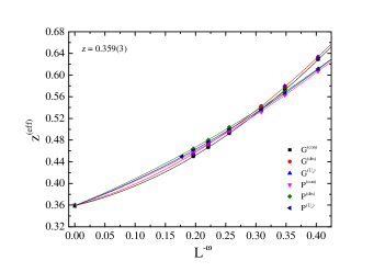
Finally, we discuss some computational aspects of the implemented push-relabel algorithm and its performance on the study of the RFIM. Although its generic implementation has a polynomial time bound, its actual performance depends on the order in which operations are performed and which heuristics are used to maintain auxiliary fields for the algorithm. Even within this polynomial time bound, there is a power-law critical slowing down of the push-relabel algorithm at the zero-temperature transition Ogielski (1985). A direct way to measure the dynamics of the algorithm is to examine the dependence of the running time, measured by the number of push-relabel operations, on system size $L$ Middleton (2001); Middleton and Fisher (2002); Middleton (2002). Such an analysis has been carried out for the 3D and 4D versions of the model and a FIFO (first in, first out) queue implementation Middleton (2001); Middleton and Fisher (2002); Middleton (2002); Fytas and Martín-Mayor (2016); Fytas et al. (2016b). We present here results for the performance of the algorithm on the 5D RFIM using our scaling approach within the quotients method and numerical data for both Gaussian and Poissonian random-field distributions. In Fig. 8 we plot the effective exponent values of $z$ at the various crossing points considered, as indicated in the panel. The solid line is a joint quadratic ($a_{3}=0$) fit of the form (6) with $\omega=0.66$. The obtained estimate for the dynamic critical exponent is $z=0.359(3)$, as marked by the filled star at $L^{-\omega}=0$.

IV Summary of results for the RFIM at $3\leq D<6$

We find it most useful to present in this last Section a summary of the most recent computations of the critical properties of the RFIM at three and higher dimensions by our group Fytas and Martín-Mayor (2013, 2016); Fytas et al. (2016a, b), still below the upper critical dimensionality $D_{\rm u}=6$. Our presentation will take place under the prism of the original prediction of dimensional reduction, by contrasting the critical exponents of the $D$-dimensional RFIM to those of the pure $D-2$ Ising ferromagnet. The current numerical data at hand will also allow us to further verify some of the most controversial scaling relations in the literature of the RFIM, that is the Rushbrooke relation $\alpha+2\beta+\gamma=2$. In doing so, we will make use of some standard exponent relations to provide estimates for the complete spectrum of critical exponents.

In particular:

• The violation of the hyperscaling exponent $\theta$ may be estimated via the anomalous dimensions $\eta$ and $\bar{\eta}$ as $\theta=2-\bar{\eta}+\eta=2-\eta+\Delta_{\eta,\bar{\eta}}$, where $\Delta_{\eta,\bar{\eta}}=2\eta-\bar{\eta}$.

• We note here also the relation of $\theta$ to the critical exponent $\alpha$ of the specific heat via the modified hyperscaling relation $(D-\theta)\nu=2-\alpha$, which then leads to $\alpha=2-\nu(D-2+\eta-\Delta_{\eta,\bar{\eta}})$.

• Finally, for the estimation of the magnetic critical exponents $\beta$ and $\gamma$ we have used the standard relations $\beta=\nu(D-4+\bar{\eta})/2$ and $\gamma=\nu(2-\eta)$.

In Tab. 3 we present all our results for the critical exponents, critical points, and universal ratios of the RFIM at $D=3$, $4$, and $D=5$. The first and most striking observation is that the critical exponents of the 4D RFIM have a clear deviation when compared to those of the 2D Ising ferromagnet indicating the breaking of dimensional reduction at the dimensionality $D=4$ and pointing at $D_{\rm int}>4$, as has already been stressed in Ref. Fytas et al. (2016a). On the other hand, the deviation from the supersymmetry ($\eta=\bar{\eta}$ or $\theta=2$) clearly decreases with increasing $D$ and our numerical results at five dimensions are compatible, within statistical accuracy, to a restoration of the supersymmetry at $D=5$ (see also the statistical tests presented in Tab. 2 that support our claim). As discussed above, the measured exponents of the 5D RFIM are close to those of the pure 3D Ising ferromagnet, but not exactly the same when it comes to the anomalous dimensions. This still leaves open the possibility that the restoration takes places at a (non-physical) real value of $D$ slightly larger than $5$ and not exactly at $D=5$. Another important remark of Tab. 3 is that our numerical estimates for the critical exponents $\alpha$, $\beta$, and $\gamma$, satisfy the Rushbrooke relation up to a very high accuracy and at all studied dimensions $D=3$, $4$, and $D=5$.

So, where do we stand at this point? Clearly, we have now at hand a complete picture of the model’s critical behavior for $D<D_{\rm u}$. This includes very accurate estimates of the full spectrum of critical exponents, critical points, and universal ratios, as well as an unarguable claim of universality and the verification of scaling relations. These latter concepts have been severely questioned in the study of the random-field problem but now seem to be perfectly settled. What may be seen as a further step in the study of the random-field problem would be a detailed investigation of criticality at the suspected upper critical dimension $D_{\rm u}=6$, for which characteristic logarithmic scaling violations have been reported Ahrens and Hartmann (2011), but still await for a detailed confirmation.

To conclude, let us point out that the questions addressed in this paper are of interest for the properties of phase transitions of disordered systems in general, and not only for the RFIM. Still, the RFIM is unique among other models due to the existence of very fast algorithms that make the study of these questions numerically feasible.