Axion, $\mu$ Term, and Supersymmetric Hybrid Inflation

Abstract

We show how successful supersymmetric hybrid inflation is realized in realistic models where the resolution of the minimal supersymmetric standard model $\mu$ problem is intimately linked with axion physics. The scalar fields that accompany the axion, such as the saxion, are closely monitored during and after inflation to ensure that the axion isocurvature perturbations lie below the observational limits. The scalar spectral index $n_{\rm s}\simeq 0.96-0.97$, while the tensor-to-scalar ratio $r$, a canonical measure of gravity waves, lies well below the observable range in our example. The axion domain walls are inflated away, and depending on the axion decay constant $f_{\rm a}$ and the magnitude of the $\mu$ parameter, the axions and/or the lightest supersymmetric particle compose the dark matter in the universe. Non-thermal leptogenesis is naturally implemented in this class of models.

I Introduction

An attractive feature of the simplest supersymmetric (SUSY) hybrid inflation models dvali ; copeland (for a review see e.g., Ref. lectures ) is the prediction that, to a good approximation, the temperature anisotropy $\delta T/T$ of the cosmic microwave background radiation is proportional to $(M/m_{\rm P})^{2}$ dvali , where $M$ denotes the scale of the gauge symmetry breaking associated with inflation and $m_{\rm P}\simeq 2.44\times 10^{18}~{}{\rm GeV}$ denotes the reduced Planck mass. Thus, $M$ is comparable to or somewhat smaller than the SUSY grand unified theory (GUT) scale $M_{\rm GUT}$. Moreover, the scalar spectral index $n_{\rm s}$ lies in the observed range of 0.96-0.97 planckcosm provided the inflationary potential incorporates, in addition to radiative corrections dvali , either the soft SUSY breaking terms rehman ; gravitywaves or higher order terms in the Kähler potential bastero . In the absence of these terms the spectral index $n_{\rm s}$ lies close to 0.98, which seems acceptable provided the effective number of light neutrino species is slightly higher than 3 planckcosm . Note that in either case the supergravity corrections remain under control because the 55 or so e-foldings necessary to resolve the horizon and flatness problems are realized for inflaton values well below the Planck scale $m_{\rm P}$. Finally, the initial condition problem of hybrid inflation can be solved initial by invoking two stages of inflation.

In this paper, we propose to merge SUSY hybrid inflation with axion physics, which provides PecceiQuinn the most compelling resolution of the strong CP problem. We incorporate in our discussion the nice feature that the intermediate ($M_{\rm I}\sim 10^{11}-10^{12}~{}{\rm GeV}$ preskill ) spontaneous symmetry breaking scale of the global $U(1)$ axion symmetry can be exploited nilles to resolve the $\mu$-term problem of the minimal supersymmetric standard model (MSSM). Namely, the usual MSSM $\mu$ term is forbidden through a combination of the underlying symmetries, but it arises from a higher dimensional superpotential term. The resulting value of $\mu$ turns out to be of order $M_{\rm I}^{2}/m_{\rm P}\sim{\rm TeV}$, the desired magnitude. The scalar spectral index $n_{\rm s}$ is adjusted to the observed range by using higher order terms in the Kähler potential. The tensor-to-scalar ratio $r$ turns out to be negligible in this simple hybrid inflation model. Appreciable values of $r$ could, however, be achieved if one replaces this model by a two stage hybrid inflation scenario dinf .

Note that this extension of the MSSM with matter parity allows for the possible presence of more than a single species of cold dark matter. With a suitable choice of the parameters both the axion and the lightest supersymmetric particle (LSP) would contribute to the dark matter density in the universe. For a recent discussion of natural SUSY in the framework of axion physics see Ref. baer and references therein.

In particular, in this work, we investigate how the Peccei-Quinn (PQ) or axion transition proceeds in a SUSY model with hybrid inflation without creating any problems with the observations. A potential problem is the generation of unacceptably large axion isocurvature perturbations. The avoidance of such perturbations requires that the value of the PQ field during inflation be kept fairly large, which can be achieved by appropriately using higher order terms in the Kähler potential. These terms produce a suitable negative mass-squared term for the PQ field and thereby shift its vacuum value to become appropriately large during inflation. Consequently, the value of the PQ field remains large during inflation. It also remains large but time-dependent during the inflaton oscillations which follow inflation and gradually drifts to the desired low energy PQ vacuum. As a consequence, the PQ symmetry is spontaneously broken already during inflation and remains so thereafter. Therefore, the axion domain wall problem sikivie , which appears if the spontaneous breaking of the PQ symmetry takes place after inflation, does not arise here. For a different approach to avoid domain walls in axion models see Ref. yanagida .

A thorough numerical investigation over several orders of magnitude in cosmic time shows how the PQ field value develops during inflation and the subsequent inflaton oscillations until low energies where the soft SUSY breaking terms take over. We estimate the amplitude of the PQ oscillations when this regime is reached in order to calculate the ensuing relic saxion abundance. Note that the system contains not only the saxion and the axion but also an extra complex Higgs field and a four component Dirac axino. Under certain conditions, one can show that the extra Higgs field does not perform any appreciable oscillations which could contribute to the energy density of the universe.

The decay time of the various states of the PQ system and the relic density of the thermally produced saxions, axinos, and extra Higgs particles have been estimated too. The possible contribution of the axinos as well as the axions to the cold dark matter of the universe is briefly explored.

The layout of the paper is as follows. In Sec. II, we investigate the PQ transition in the context of SUSY hybrid inflation. In Sec. III, we estimate the relic density of the various PQ states. Sec. IV is devoted to the discussion of the axion isocurvature perturbations and our conclusions are summarized in Sec. V.

II Model and the PQ transition

For definiteness, we consider a SUSY model based on the left-right symmetric gauge group $G_{\rm{LR}}=SU(3)_{\rm c}\times SU(2)_{\rm L}\times SU(2)_{\rm R}\times U(1)_{B-L}$. The superfield content of the model comprises the gauge singlets $S$, $N$, $\bar{N}$, the Higgs superfields $H$, $\bar{H}$, $h$ belonging to the $(1,1,2)_{1}$, $(1,1,2)_{-1}$, $(1,2,2)_{0}$ representation of $G_{\rm{LR}}$, respectively, and the matter superfields $q_{i}$, $q^{c}_{i}$, $l_{i}$, $l^{c}_{i}$ (with $i=1,2,3$) which belong to the $(3,2,1)_{\frac{1}{3}}$, $(\bar{3},1,2)_{-\frac{1}{3}}$, $(1,2,1)_{-1}$, $(1,1,2)_{1}$ representation of $G_{\rm LR}$, respectively. Here the subscripts denote $U(1)_{B-L}$ charges. The fields $H$ and $\bar{H}$ acquire vacuum expectation values (VEVs), which cause the breaking of $G_{\rm LR}$ to the standard model (SM) gauge group $G_{\rm SM}$, while the VEV of $h$ is responsible for the electroweak symmetry breaking.

The global symmetries imposed on the model include a R symmetry $U(1)_{\rm R}$ under which the superfields have the following charge assignments

$$R: S(2),N(0),\bar{N}(2),H(0),\bar{H}(0),h(1),$$ (1)

$$q_{i}(0),q^{c}_{i}(1),l_{i}(0),l^{c}_{i}(1)$$

with the superpotential having charge 2, and a PQ symmetry $U(1)_{\rm{PQ}}$ under which the superfields have the following charges

$$PQ: S(0),N(-1),\bar{N}(3),H(0),\bar{H}(0),h(1),$$ (2)

$$q_{i}(-1),q^{c}_{i}(0),l_{i}(-1),l^{c}_{i}(0).$$

The above charge assignments allow in the superpotential the usual Yukawa couplings for quarks and leptons as well as the higher order terms $\bar{H}\bar{H}l^{c}_{i}l^{c}_{j}$ which provide intermediate scale right-handed neutrino masses. Moreover, the MSSM $\mu$ term $h^{2}$ is forbidden, but the term $N^{2}h^{2}$ is allowed and generates, as we will see, a $\mu$ term of the desired magnitude.

The soft SUSY breaking terms break the $U(1)_{\rm R}$ symmetry explicitly to its $Z_{2}$ subgroup under which $h$, $q^{c}_{i}$, and $l^{c}_{i}$ change sign. This symmetry, combined with the $Z_{2}$ center of $SU(2)_{\rm L}$ under which $h$, $q_{i}$, and $l_{i}$ flip sign, provides the well-known $Z_{2}^{\rm mp}$ matter parity symmetry under which the matter fields $q_{i}$, $q^{c}_{i}$, $l_{i}$, and $l^{c}_{i}$ are odd. Consequently, the apparent spontaneous breaking by the VEV of $h$ of the $Z_{2}$ subgroup of $U(1)_{\rm R}$ which is left unbroken after soft SUSY breaking does not lead to the cosmologically unacceptable production of domain walls. In reality, this $Z_{2}$ symmetry is merely replaced by the equivalent $Z_{2}^{\rm mp}$, which remains unbroken. In addition, the $U(1)_{\rm PQ}$ symmetry is broken explicitly by QCD instantons to its $Z_{6}$ subgroup. However, the spontaneous breaking of this discrete symmetry does not cause any trouble with domain walls. The reason is that, as we will demonstrate in the following, this breaking occurs already during inflation and the walls are inflated away.

It is worth noting that, as a consequence of the field content and the symmetries imposed, our simple model exhibits, excluding non-perturbative effects, exact baryon number conservation as an accidental symmetry.

The superpotential component which is relevant for inflation and the evolution of the PQ system is

$$W=\kappa S\left(M^{2}-H{\bar{H}}\right)+\frac{\lambda}{m_{\rm P}}N^{3}\bar{N},$$ (3)

and the Kähler potential is taken to be

$$K=|S|^{2}+|H|^{2}+|\bar{H}|^{2}+|N|^{2}+|\bar{N}|^{2}+\frac{\alpha}{4m_{\rm P}^{2}}|S|^{4}+$$

$$\left(c_{1}|S|^{2}+c_{2}|H|^{2}+c_{3}|\bar{H}|^{2}+c_{4}\left(H\bar{H}+h.c.\right)\right)\frac{|N|^{2}}{m_{\rm P}^{2}}+$$

$$\left(c_{5}|S|^{2}+c_{6}|H|^{2}+c_{7}|\bar{H}|^{2}+c_{8}\left(H\bar{H}+h.c.\right)\right)\frac{|\bar{N}|^{2}}{m_{\rm P}^{2}}.$$

Here $M$ is a superheavy mass and $\kappa$, $\lambda$, $\alpha$, $c_{1}$, $c_{2}$, $c_{3}$, $c_{4}$, $c_{5}$, $c_{6}$, $c_{7}$, $c_{8}$ are dimensionless constants which are all taken to be real. In addition, we assume that $\alpha>0$ and $c_{1}>1$, $c_{2}$, $c_{3}\geq 1$, while $c_{5}$, $c_{6}$, $c_{7}<1$. The motivation for this assumption will become clear later. Note that the superpotential in Eq. (3) was first introduced in Ref. intermediate for achieving the PQ transition after the termination of inflation without runaway problems.

Expanding the F-term potential in powers of $m_{\rm P}^{-1}$ and keeping terms up to $m_{\rm P}^{-2}$, we obtain

$$V = \kappa^{2}|M^{2}-H\bar{H}|^{2}\left(1+|H|^{2}+|\bar{H}|^{2}-\alpha|S|^{2}-\right.$$

$$\left.(c_{1}-1)|N|^{2}+(1-c_{5})|\bar{N}|^{2}\right)+$$

$$\kappa^{2}|S|^{2}\left(|H|^{2}+|\bar{H}|^{2}\right)\left(1+|S|^{2}+|H|^{2}+|\bar{H}|^{2}\right)+$$

$$4\kappa^{2}|S|^{2}|H|^{2}|\bar{H}|^{2}-2\kappa^{2}M^{2}|S|^{2}\left(H\bar{H}+h.c.\right)-$$

$$\kappa^{2}|S|^{2}\left((c_{3}-1)|H|^{2}+(c_{2}-1)|\bar{H}|^{2}\right)|N|^{2}+$$

$$\kappa^{2}|S|^{2}\left((1-c_{7})|H|^{2}+(1-c_{6})|\bar{H}|^{2}\right)|\bar{N}|^{2}+$$

$$\lambda^{2}|N|^{4}\left(|N|^{2}+9|\bar{N}|^{2}\right)+$$

$$m_{{3}/{2}}^{2}\left(\varepsilon_{1}|N|^{2}+\varepsilon_{2}|\bar{N}|^{2}\right)+m_{{3}/{2}}\left(\lambda AN^{3}\bar{N}+h.c.\right).$$

Here we have included the soft SUSY breaking terms associated only with the fields $N$ and $\bar{N}$ and have chosen units in which the reduced Planck mass scale $m_{\rm P}=1$, which we will use in the rest of the paper. Notice that in this approximation the parameters $c_{4}$, $c_{8}$ do not enter the potential.

For simplicity, in the following we set $A=0$ for the parameter of the trilinear soft SUSY breaking terms. We also take $\varepsilon_{2}>0$ for the soft SUSY breaking mass-squared term associated with the field $\bar{N}$. Then, it is apparent that, with our assumption that $c_{5}$, $c_{6}$, $c_{7}<1$, $\bar{N}$ enters the potential through a positive definite quadratic term and, as a consequence, the minimum of the potential is obtained for $\bar{N}=0$ independent of the values of the remaining fields. Therefore, we may safely set $\bar{N}=0$ throughout the rest of our discussion, which considerably simplifies our analysis. With $\bar{N}$ set to zero, the parameter $\varepsilon_{1}$ may be absorbed into a redefinition of $m_{{3}/{2}}^{2}$ once the choice of its sign is made. In order to achieve spontaneous breaking of the PQ symmetry, we choose $\varepsilon_{1}<0$. Moreover, the SUSY minimum of the potential (obtained in the limit $m_{{3}/{2}}\rightarrow 0$) lies along the D-flat direction $H=\bar{H}^{*}$ to which we restrict our analysis.

Using the $U(1)_{\rm R}$, $U(1)_{\rm{PQ}}$, and $U(1)_{B-L}$ symmetries of the model, we can rotate $S$, $N$, $H$, and, on account of the D-flatness, $\bar{H}$ on the real axis. Then, provided that the values of the fields remain well below unity in size, we define almost canonically normalized real scalar fields $\sigma$, $\chi$, and $h$ as follows

$$S=\frac{\sigma}{\sqrt{2}},\quad N=\frac{\chi}{\sqrt{2}},\quad H=\bar{H}=\frac{h}{2}.$$ (6)

In terms of the fields $\sigma$, $\chi$, and $h$, the potential becomes

$$V = \kappa^{2}\left(M^{2}-\frac{h^{2}}{4}\right)^{2}\left(1+\frac{h^{2}}{2}-\alpha\frac{\sigma^{2}}{2}-d_{1}\frac{\chi^{2}}{2}\right)+$$ (7)

$$\frac{\kappa^{2}}{4}\sigma^{2}h^{2}\left(1+\frac{\sigma^{2}}{2}+h^{2}-2M^{2}-d_{2}\frac{\chi^{2}}{2}\right)+$$

$$\frac{\lambda^{2}}{8}\chi^{6}-\frac{1}{2}m_{{3}/{2}}^{2}\chi^{2},$$

where

$$d_{1}\equiv c_{1}-1>0$$ (8)

and

$$d_{2}\equiv\frac{c_{2}+c_{3}}{2}-1\geq 0.$$ (9)

The part of the potential involving the field $\chi$ may be written as

$$V_{\chi}=-\frac{1}{2}m_{\chi}^{2}\chi^{2}+\frac{\lambda^{2}}{8}\chi^{6},$$ (10)

where

$$m_{\chi}^{2}=d_{1}\,\kappa^{2}\left(M^{2}-\frac{h^{2}}{4}\right)^{2}+d_{2}\,\frac{\kappa^{2}}{4}\sigma^{2}h^{2}+m_{{3}/{2}}^{2}.$$ (11)

$V_{\chi}$ is minimized for values $\chi_{\rm m}$ of $\chi$ satisfying

$$|\chi_{\rm m}|=\sqrt{2}\left(\frac{m_{\chi}^{2}}{3\lambda^{2}}\right)^{\frac{1}{4}}.$$ (12)

Note that the positivity of $d_{1}$, and non-negativity of $d_{2}$, which are consequences of our assumption that $c_{1}>1$, $c_{2}$, $c_{3}\geq 1$, guarantee the positivity of $m_{\chi}^{2}$ in Eq. (11). As a result, during inflation, the subsequent inflaton oscillations, and after reheating, the minimum of the potential is shifted away from $\chi=0$. This is crucial for controlling the axion isocurvature perturbations and avoiding the axion domain wall problem (see Sec. IV).

If $\sigma$ satisfies the inequality $\sigma^{2}>\sigma_{\rm c}^{2}\simeq 2M^{2}$, the $\sigma$-dependent mass squared $m_{h}^{2}\simeq\kappa^{2}(\sigma^{2}-2M^{2})/2$ of $h$ is positive, thus, rendering the choice $h=0$ stable. With $h=0$ the potential becomes

$$V\overset{h=0}{=}\kappa^{2}M^{4}\left(1-\alpha\frac{\sigma^{2}}{2}\right)+V_{\chi}\simeq\kappa^{2}M^{4},$$ (13)

leading to a hybrid inflationary stage. In addition, we have

$$m_{\chi}^{2}=d_{1}\kappa^{2}M^{4}+m_{{3}/{2}}^{2}\simeq d_{1}\kappa^{2}M^{4}$$ (14)

and, as a consequence, $|\chi_{\rm m}|$ during inflation becomes

$$|\chi_{\rm inf}|\simeq\sqrt{2}\left(\frac{d_{1}\kappa^{2}M^{4}}{3\lambda^{2}}\right)^{\frac{1}{4}}.$$ (15)

Since $m_{\chi}$ is of the order of the inflationary Hubble parameter, $\chi$ is expected to quickly reach the above value. With such a value of $\chi$ it can be verified that $V_{\chi}\ll\kappa^{2}M^{4}$ and the approximation made is justified.

To the inflationary potential we add the contribution

$$V_{\rm{rad}}=\kappa^{2}M^{4}\left(\frac{\delta_{h}}{2}\right)\ln\frac{\sigma^{2}}{\sigma_{\rm c}^{2}}$$ (16)

from radiative corrections, where

$$\delta_{h}=N_{h}\frac{\kappa^{2}}{8\pi^{2}}$$ (17)

and $N_{h}=2$ is the dimensionality of the representation to which $H$, $\bar{H}$ belong. Note that this equation holds for $\sigma/\sigma_{\rm c}\gg 1$, which requires that $|\kappa|$ be not much smaller than about $0.01$. The potential during inflation is then

$$V_{\rm{inf}}\simeq\kappa^{2}M^{4}\left(1+\frac{\delta_{h}}{2}\ln\frac{\sigma^{2}}{\sigma_{\rm c}^{2}}-\alpha\frac{\sigma^{2}}{2}\right)\simeq\kappa^{2}M^{4}.$$ (18)

The first, second, and third derivative of $V_{\rm inf}$ with respect to the inflaton field $\sigma$ are, respectively, given by

$$V_{\rm{inf}}^{\prime}=\kappa^{2}M^{4}\left(\frac{\delta_{h}}{\sigma}\right)\left(1-\frac{\alpha\sigma^{2}}{\delta_{h}}\right),$$ (19)

$$V_{\rm{inf}}^{\prime\prime}=-\kappa^{2}M^{4}\left(\frac{\delta_{h}}{\sigma^{2}}\right)\left(1+\frac{\alpha\sigma^{2}}{\delta_{h}}\right),$$ (20)

and

$$V_{\rm{inf}}^{\prime\prime\prime}=2\kappa^{2}M^{4}\frac{\delta_{h}}{\sigma^{3}}.$$ (21)

Introducing the parameter $x$

$$x\equiv\frac{\alpha\sigma^{2}}{\delta_{h}}<1,$$ (22)

we obtain the slow-roll parameters

$$\epsilon\equiv\frac{1}{2}\left(\frac{V_{\rm inf}^{\prime}}{V_{\rm inf}}\right)^{2}\simeq\frac{1}{2}\alpha\delta_{h}\frac{(1-x)^{2}}{x},$$ (23)

$$\eta\equiv\frac{V_{\rm{inf}}^{\prime\prime}}{V_{\rm inf}}\simeq-\alpha\frac{1+x}{x},$$ (24)

and

$$\xi\equiv\left(\frac{V_{\rm{inf}}^{\prime}}{V_{\rm inf}}\right)\left(\frac{V_{\rm{inf}}^{\prime\prime\prime}}{V_{\rm{inf}}}\right)\simeq 2\alpha^{2}\frac{1-x}{x^{2}}.$$ (25)

From these equations, we see that $\epsilon/|\eta|<\delta_{h}/2$ and $\epsilon|\eta|/\xi<\delta_{h}/4$. So assuming $\delta_{h}\ll 1$, we obtain $\epsilon\ll|\eta|$ and $\epsilon|\eta|\ll\xi$.

Inflation ends when $\sigma$ reaches the value $\sigma_{\rm{end}}$ with

$$\sigma_{\rm{end}}^{2}\simeq\max\{2M^{2},\delta_{h}\},$$ (26)

depending on whether termination of inflation occurs through the waterfall mechanism or because of the radiative corrections becoming strong ($|\eta|\simeq 1$). The number ${\bf N}(x_{\rm{in}})$ of e-foldings in the slow-roll approximation for the period in which $\sigma$ varies between an initial value $\sigma_{\rm{in}}$ and the final value $\sigma_{\rm{end}}$ corresponding, respectively, to the values $x_{\rm{in}}$ and

$$x_{\rm{end}}\simeq\alpha\max\{\frac{2M^{2}}{\delta_{h}},1\}$$ (27)

of the variable $x$ is given by

$${\bf N}(x_{\rm{in}})\simeq\frac{1}{2\alpha}\ln\frac{1-x_{\rm{end}}}{1-x_{\rm{in}}}.$$ (28)

Let the value of the inflaton field $\sigma$ at horizon exit of the pivot scale $k_{*}=0.05\ \rm{Mpc}^{-1}$ be $\sigma_{*}$, with $x_{*}$ being the corresponding value of the parameter $x$. Let us also assume that

$$x_{\rm{end}}\ll x_{*}.$$ (29)

Then,

$${\bf N}_{*}\equiv{\bf N}(x_{*})\simeq\frac{1}{2\alpha}\ln\frac{1}{1-x_{*}},$$ (30)

which implies that

$$\alpha\simeq\frac{1}{2{\bf N}_{*}}\ln\frac{1}{1-x_{*}}.$$ (31)

Moreover, the scalar spectral index $n_{\rm s}$ is obtained in terms of $\eta_{*}$, the slow-roll parameter $\eta$ evaluated at the value $x=x_{*}$, as follows:

$$n_{\rm s} \simeq 1+2\eta_{*}$$ (32)

$$\simeq 1-2\alpha\frac{1+x_{*}}{x_{*}}$$

$$\simeq 1-\frac{1}{{\bf N}_{*}}\left(\frac{1+x_{*}}{x_{*}}\ln\frac{1}{1-x_{*}}\right).$$

Its running $\alpha_{\rm s}\equiv dn_{\rm s}/d\ln{k}$ is

$$\alpha_{\rm s}\simeq-2\xi_{*}\simeq-4\alpha^{2}\frac{1-x_{*}}{x_{*}^{2}},$$ (33)

where $\xi_{*}$ is the parameter $\xi$ evaluated at horizon exit of the pivot scale. Finally, the scalar potential on the inflationary path can be written in terms of the scalar power spectrum amplitude $A_{\rm s}$ and the value $\epsilon_{*}$ of the slow-roll parameter $\epsilon$, both evaluated at horizon exit of the pivot scale, as

$$V=24\pi^{2}\epsilon_{*}A_{\rm s},$$ (34)

from which we obtain

$$M^{4}\simeq 3\alpha\left(\frac{N_{h}}{2}\right)\frac{(1-x_{*})^{2}}{x_{*}}A_{\rm s}.$$ (35)

Many SUSY inflation scenarios predict the relation $n_{\rm s}\simeq 1-1/{\bf N}_{*}$ (see e.g., Ref. dvali ), which gives $n_{\rm s}$ values close to 0.98, instead of the presently favored values which are close to 0.96 planckcosm . For three neutrino species, a modified relation $n_{\rm s}\simeq 1-2/{\bf N}_{*}$ is in better agreement with recent observations. Such a relation is easily obtained in our model if we choose for $x_{*}$ a value close to 0.5. Indeed, setting $x_{*}=0.5$ and ${\bf N}_{*}=52$, for solving the horizon and flatness problems for reheat temperature $T_{\rm r}\sim 10^{9}~{}{\rm GeV}$, we obtain $\alpha\simeq 1/150$, $n_{\rm s}\simeq 0.96$, $\alpha_{\rm s}\simeq-3.56\times 10^{-4}$, and $M\simeq 2.17\times 10^{-3}$, setting $N_{h}=2$ and $A_{\rm s}=2.215\times 10^{-9}$ planckcosm .

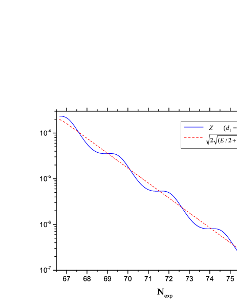
Figure 1: Postinflationary evolution of the field $\chi$ as a function of the number of e-foldings ${\bf N}_{\rm exp}$ for $m_{3/2}=10^{-14}$ and $d_{1}=d_{2}=1$. The moving position in Eq. (38) of the minimum of the potential is also depicted.

Figure 2: Postinflationary evolution of the field $\chi$ as a function of the number of e-foldings ${\bf N}_{\rm exp}$ for $m_{3/2}=10^{-13}$ and $d_{1}=d_{2}=1$. The moving position in Eq. (38) of the minimum of the potential is also depicted.

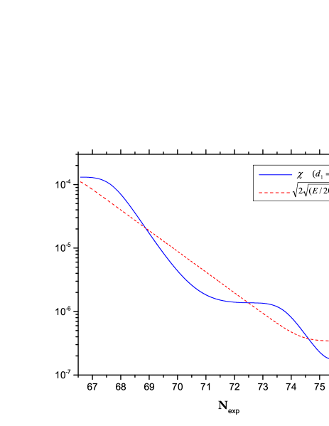
Figure 3: Postinflationary evolution of the field $\chi$ as a function of the number of e-foldings ${\bf N}_{\rm exp}$ for $m_{3/2}=10^{-13}$ and $d_{1}=d_{2}=0.1$. The moving position in Eq. (38) of the minimum of the potential is also depicted.

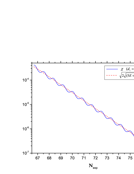
Figure 4: Postinflationary evolution of the field $\chi$ as a function of the number of e-foldings ${\bf N}_{\rm exp}$ for $m_{3/2}=10^{-13}$ and $d_{1}=d_{2}=10$. The moving position in Eq. (38) of the minimum of the potential is also depicted.

So far we have not determined the coupling constant $\kappa$. Its value enters our considerations indirectly since it only controls the size of terms that we have neglected. From Eqs. (17) and (27), we see that inflation terminates via the waterfall mechanism provided $\kappa^{2}\lesssim 8\pi^{2}M^{2}\simeq 3.72\times 10^{-4}$. In this case, with $\kappa^{2}$ decreasing, $x_{\rm{end}}$ increases and, thus, the neglected term $(1/2\alpha)\ln(1-x_{\rm{end}})$ in Eq. (30) increases in magnitude and, if included, leads to a larger reduction of ${\bf N}_{*}$. With increasing $\kappa^{2}$, instead, $\sigma_{*}^{2}$ increases and higher order terms in the potential which have not been taken into account start to play a role. As a suitable compromise, we may choose the value $\kappa=0.01$ yielding $|\sigma_{*}|=\sqrt{\delta_{h}x_{*}/\alpha}\simeq 0.01378$, $x_{\rm{end}}\simeq 0.0248$, and $\epsilon_{*}\simeq 4.22\times 10^{-9}$. So the tensor-to-scalar ratio

$$r=16\epsilon_{*}$$ (36)

turns out to be about $6.76\times 10^{-8}$ implying that gravity waves are not observable in this case. Observable gravity waves in SUSY hybrid inflation have been discussed in Ref. gravitywaves . Taking into account the correction to ${\bf N}_{*}$ from $x_{\rm{end}}$, we obtain ${\bf N}_{*}\simeq 50.1$. If we also include the effect of the term $\propto\sigma^{4}$ in the inflationary potential, ${\bf N}_{*}$ is slightly reduced to ${\bf N}_{*}\simeq 49.9$, while $n_{\rm s}$ increases slightly to $n_{\rm s}\simeq 0.9606$.

To facilitate the theoretical analysis of the evolution of the field $\chi$ after the end of inflation, it is convenient to assume that $d_{1}=d_{2}=d$ (choosing e.g., $c_{1}=c_{2}=c_{3}$). In this case,

$$m_{\chi}^{2}\simeq d\,V+m_{{3}/{2}}^{2},$$ (37)

provided that $V_{\chi}\ll V$. During the period following the end of inflation and before reheating, the energy density $E$ is dominated by the energy density of the rapidly oscillating massive fields $\sigma$ and $h$. Then, we may approximate $V$ in the above expression for $m_{\chi}^{2}$ with its average value during one oscillation which is expected to be equal to $E/2$. Thus, we are led to the approximate expression

$$|\chi_{\rm m}|\simeq\sqrt{2}\left(\frac{d\,E/2+m_{{3}/{2}}^{2}}{3\lambda^{2}}\right)^{\frac{1}{4}}$$ (38)

for the position of the minimum of the potential $V_{\chi}$ in terms of the energy density $E$. As $d\,E/2$ approaches $m_{{3}/{2}}^{2}$, the decrease of $|\chi_{\rm m}|$ becomes slower until it reaches smoothly the value

$$|\left<\chi\right>|=\sqrt{2}|\left<N\right>|\equiv f_{\rm a}=\sqrt{2}\left(\frac{m_{{3}/{2}}^{2}}{3\lambda^{2}}\right)^{\frac{1}{4}},$$ (39)

which determines the PQ breaking scale $f_{\rm a}$ (axion decay constant).

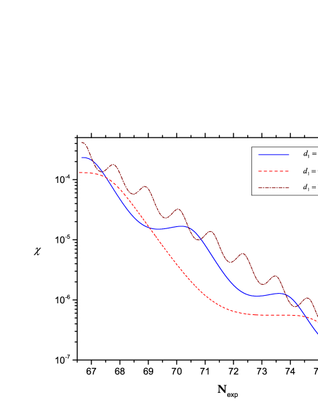
Figure 5: Postinflationary evolution of the field $\chi$ as a function of the number of e-foldings ${\bf N}_{\rm exp}$ for $m_{3/2}=10^{-13}$ and $d_{1}=1$, $0.1$, $10$ and $d_{2}=0$.

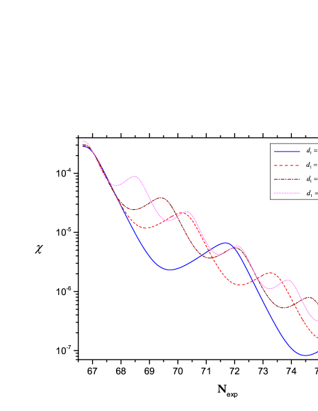
Figure 6: Postinflationary evolution of the field $\chi$ as a function of the number of e-foldings ${\bf N}_{\rm exp}$ for $m_{3/2}=10^{-13}$ and $d_{1}=2.2$, $2.5$, $3$, $5$ and $d_{2}=-1$.

In order to confirm our theoretical analysis concerning the postinflationary evolution of the field $\chi$, we solve numerically the differential equations describing the dynamics of the system with potential energy density given in Eq. (7) and the following choice of parameters: $\kappa=0.01$, $\lambda=1$, $\alpha=1/150$, and $M=2.17\times 10^{-3}$. As initial conditions, we set: $\sigma=0.015$, $\dot{\sigma}=-1.86\times 10^{-12}$, $h=10^{-8}$, $\dot{h}=0$, $\chi=10^{-5}$, $\dot{\chi}=0$ (overdot denotes derivation with respect to cosmic time). The initial velocity of $\sigma$ is the actual value of its velocity on the inflationary path, which was determined numerically. We followed the evolution of the system for 77 e-foldings of expansion out of which approximately 66.7 correspond to inflationary expansion. Notice that the initial value of $\sigma$ is larger than $|\sigma_{*}|$. The value of the final energy density after 77 e-foldings of expansion is close to $10^{-28}$.

In Figs. 1-4, we plot the values of the field $\chi$ and the varying value of $|\chi_{\rm m}|$ in Eq. (38) as functions of the number of e-foldings ${\bf N}_{\rm exp}$ only for the period following the end of inflation. Note that the number of e-foldings ${\bf N}_{\rm exp}$ is measured starting from the cosmic time at which the initial conditions were imposed. In Fig. 1, $m_{3/2}=10^{-14}$ while in all other figures $m_{3/2}=10^{-13}$. Moreover, in Figs. 1 and 2, $d_{1}=d_{2}=1$, in Fig. 3, $d_{1}=d_{2}=0.1$, and, in Fig. 4, $d_{1}=d_{2}=10$. We see that $\chi$ oscillates around the moving position $\chi_{\rm m}$ of the minimum in Eq. (38) adjusting faster to it when $d$ is larger. Also, in Fig. 1, $\chi_{\rm m}$ after 77 e-foldings has just started approaching the value of the PQ vacuum of Eq. (39), while in all other figures it essentially has reached the value of Eq. (39) and the amplitude of the oscillations of $\chi$ has been severely reduced. Our numerical findings are in accord with our theoretical expectations. It should be noted that, reducing the parameter $\lambda$ below 1, $\chi_{\rm m}$ is just rescaled by a factor $\lambda^{-1/2}$ as one can see from Eq. (12). Consequently, in all these figures, $\chi$ is practically just multiplied by the same factor. This is confirmed numerically too.

Encouraged by the good agreement of the numerical results with our theoretical expectations so far, we also consider the limiting case $d_{2}=0$, but insisting that $d_{1}>0$ in order that $|\chi|$ have an appreciable value during inflation. In Fig. 5, we plot the postinflationary evolution of the field $\chi$ versus ${\bf N}_{\rm exp}$ for $m_{3/2}=10^{-13}$ and three values of $d_{1}$, namely $d_{1}=1$, $0.1$, $10$ and a common $d_{2}=0$. We see that $\chi$ decreases oscillating with larger frequency for larger values of $d_{1}$ (larger $m_{\chi}^{2}$) until it approaches the PQ vacuum where the amplitude of the oscillations dies out. We finally allow in the numerical investigation even negative values of $d_{2}$, but always with $d_{1}>0$. Such values of $d_{2}$ can be obtained by assuming that $c_{2}$, $c_{3}<1$. In Fig. 6, we made the choices $d_{1}=2.2$, $2.5$, $3$, $5$ with a common $d_{2}=-1$ (corresponding to $c_{2}=c_{3}=0$) and the same value of $m_{3/2}$ as in Fig. 5. The emerging picture is roughly the same. Notice that in this case there are also negative contributions to $m_{\chi}^{2}$, which reduce its value and with it the absolute value of the position of the variable minimum of $V_{\chi}$ during the postinflationary era. As a consequence, the oscillating field $\chi$ acquires both positive and negative values during its oscillation unless $d_{1}$ is sufficiently large. We found that this is avoided for $d_{1}$ larger than $\simeq 2.2$.

III Relic density of the PQ fields

We will now estimate the relic densities and decay times of the particles contained in the PQ system. The relevant superpotential term is

$$\delta W_{1}=\lambda N^{3}\bar{N}.$$ (40)

The resulting potential in global SUSY is

$$V=\lambda^{2}|N|^{4}(|N|^{2}+9|\bar{N}|^{2})-m_{N}^{2}|N|^{2}+m_{\bar{N}}^{2}|\bar{N}|^{2},$$ (41)

where $-m_{N}^{2}=\varepsilon_{1}m_{3/2}^{2}$, $m_{\bar{N}}^{2}=\varepsilon_{2}m_{3/2}^{2}$ are the soft masses squared of the fields $N$, $\bar{N}$ and, for simplicity, the soft A term is set to zero. In order to find the extrema of this potential we take its derivatives with respect to $|N|$, $|\bar{N}|$ and put them equal to zero:

$$\frac{\partial V}{\partial|N|} = 2(3\lambda^{2}|N|^{4}-m_{N}^{2})|N|=0,$$

$$\frac{\partial V}{\partial|\bar{N}|} = 2(9\lambda^{2}|N|^{4}+m_{\bar{N}}^{2})|\bar{N}|=0.$$ (42)

We find two extrema: one at $|N|=|\bar{N}|=0$, which is a local maximum, and one at

$$|N|=\left(\frac{m_{N}^{2}}{3\lambda^{2}}\right)^{\frac{1}{4}}\equiv\left<N\right>,\quad\quad|\bar{N}|=0,$$ (43)

which is the absolute minimum with potential energy density

$$V_{0}=-\frac{2}{3}m_{N}^{2}\left(\frac{m_{N}^{2}}{3\lambda^{2}}\right)^{\frac{1}{2}},$$ (44)

and corresponds to the PQ vacuum in Eq. (39).

Replacing $N=\left<N\right>+\delta N$ in the potential in Eq. (41) and keeping only terms quadratic in $\delta N$ and $\bar{N}$, we find

$$V = (-m_{N}^{2}+3\lambda^{2}\left<N\right>^{4})|\delta{N}|^{2}+3\lambda^{2}\left<N\right>^{4}(\delta N+\delta N^{*})^{2}$$ (45)

$$+(3m_{N}^{2}+m_{\bar{N}}^{2})|\bar{N}|^{2}.$$

Writing $\delta N=(\delta\chi+ia)/\sqrt{2}$, we obtain a real scalar field $\delta\chi$ with mass squared $m_{\delta\chi}^{2}=4m_{N}^{2}$ which is the saxion, a massless real scalar field $a$ which is the axion, and an extra complex scalar field $\bar{N}=(\bar{\chi}+i\bar{a})\sqrt{2}$ with mass squared $m_{\bar{\chi}}^{2}=3m_{N}^{2}+m_{\bar{N}}^{2}$.

The saxion predominantly decays into a pair of MSSM Higgsinos $\tilde{h}_{u}$, $\tilde{h}_{d}$ (tilde denotes SUSY partner) via the Yukawa coupling

$$-2\sqrt{2}\,\frac{\mu}{f_{\rm a}}\,\delta N\tilde{h}_{u}\tilde{d}_{d}+h.c.,$$ (46)

which originates from the superpotential term

$$\delta W_{2}=\frac{1}{2}\lambda_{\mu}N^{2}h^{2},$$ (47)

where $h=(h_{u},h_{d})$ with $h_{u}$, $h_{d}$ being the electroweak Higgs superfields which couple, respectively, to the up-type and down-type quarks. It is important to note that the superpotential term in Eq. (47) is nilles also responsible for the generation of the MSSM $\mu$ term, with $\mu=\lambda_{\mu}\left<N\right>^{2}$ after the spontaneous breaking of the PQ symmetry. The origin and the magnitude of the MSSM $\mu$ term is nicely attributed to the PQ mechanism.

The saxion decay width is estimated to be

$$\Gamma_{\rm d}\simeq\frac{1}{\pi}\left(\frac{\mu}{f_{\rm a}}\right)^{2}m_{\delta\chi}.$$ (48)

The energy density $\rho_{\delta\chi}$ from the coherent saxion field oscillations about the vacuum behaves like pressureless matter. At cosmic time $t_{\rm d}=\Gamma^{-1}_{\rm d}$ of saxion decay this density is

$$\rho_{\delta\chi}^{\rm d}=\rho_{\delta\chi}^{\rm r}\left(\frac{t_{\rm r}}{t_{\rm d}}\right)^{\frac{3}{2}},$$ (49)

where $\rho_{\delta\chi}^{\rm r}$ is the energy density of saxion oscillations at the time $t_{\rm r}$ of reheating following inflation. Here, we assumed that the universe is radiation dominated after reheating and at least up to the time of saxion decay. This will be justified a posteriori. Note also that, as it turns out, $t_{\rm r}<t_{\rm d}$ (see below).

Our numerical calculations show that the amplitude of coherent saxion oscillations about the PQ vacuum at the onset of these oscillations at cosmic time $t_{\rm osc}\sim m_{\delta\chi}^{-1}$ is of order $f_{\rm a}$. Consequently, the corresponding initial energy density is

$$\rho_{\delta\chi}^{\rm osc}\sim\frac{1}{2}\,m_{\delta\chi}^{2}f_{\rm a}^{2},$$ (50)

which implies that

$$\rho_{\delta\chi}^{\rm r}\sim\frac{1}{2}\,m_{\delta\chi}^{2}f_{\rm a}^{2}\left(\frac{t_{\rm osc}}{t_{\rm r}}\right)^{2},$$ (51)

since the universe is matter dominated between $t_{\rm osc}$ and $t_{\rm r}$. Note that $t_{\rm osc}<t_{\rm r}$ (see below).

From Eqs. (49) and (51), we then find that

$$\rho_{\delta\chi}^{\rm d}\sim\frac{1}{2\pi^{2}}\,m_{\delta\chi}^{2}f_{\rm a}^{2}\left(\frac{t_{\rm d}}{t_{\rm r}}\right)^{\frac{1}{2}}\left(\frac{\mu}{f_{\rm a}}\right)^{4}.$$ (52)

For $f_{\rm a}=10^{11}~{}{\rm GeV}$ and $\mu=m_{\delta\chi}=1~{}{\rm TeV}$, Eq. (48) yields $t_{\rm d}\simeq 3.14\times 10^{13}~{}{\rm GeV}^{-1}$. The cosmic time at reheating is given by

$$t_{\rm r}=\frac{3\,\sqrt{5}}{\sqrt{2}\,\pi\,T_{\rm r}^{2}\,g_{*}(T_{\rm r})^{\frac{1}{2}}},$$ (53)

where $T_{\rm r}$ is the reheat temperature and $g_{*}(T_{\rm r})$ denotes the effective number of massless degrees of freedom at $T_{\rm r}$. For $T_{\rm r}=10^{9}~{}{\rm GeV}$ and $g_{*}(T_{\rm r})=228.75$, this equation gives $t_{\rm r}\simeq 0.24~{}{\rm GeV}^{-1}$. From Eq. (52) we then obtain $\rho_{\delta\chi}^{\rm d}\simeq 58~{}{\rm GeV}^{4}$, which compared with the radiation energy density

$$\rho_{\rm rad}^{\rm d}=\frac{\pi^{2}}{30}\,g_{*}(T_{\rm d})\,T_{\rm d}^{4}\simeq 4.5\times 10^{9}~{}{\rm GeV}^{4}$$ (54)

at the temperature $T_{\rm d}$ of saxion decay, implies that

$$\rho_{\delta\chi}^{\rm d}\ll\rho_{\rm rad}^{\rm d}.$$ (55)

Thus, the energy density of coherent saxion oscillations never dominates the energy density of the universe. In Eq. (54), $g_{*}(T_{\rm d})$ is the effective number of massless degrees of freedom at temperature $T_{\rm d}$, which is given by

$$T_{\rm d}=\frac{3^{\frac{1}{2}}5^{\frac{1}{4}}}{2^{\frac{1}{4}}\pi^{\frac{1}{2}}t_{\rm d}^{\frac{1}{2}}g_{*}(T_{\rm d})^{\frac{1}{4}}}.$$ (56)

In our numerical example, this formula gives $T_{\rm d}\simeq 110~{}{\rm GeV}$ for $g_{*}(T_{\rm d})=95.25$. The freeze-out temperature of the LSP, which is assumed to be the lightest neutralino, is $T_{\rm f}\simeq m_{\rm LSP}/25$ freeze (for a review see Ref. neutralino ), where $m_{\rm LSP}$ is the mass of the LSP. The saxions decay before the LSPs freeze out provided that

$$m_{\rm LSP}\lesssim 1.65~{}{\rm TeV},$$ (57)

and so they do not affect the usual neutralino relic abundance since they remain subdominant until their decay.

The above argument is not complete though, since so far we only considered the energy density of the coherently oscillating saxion field and ignored the thermally produced saxions. In the present case, the thermal saxion production is dominated by processes involving the saxion-Higgsino-Higgsino coupling in Eq. (46). Unfortunately, to the best of our knowledge, there is no exact calculation of the relic thermal saxion abundance $Y_{\delta\chi}\equiv n_{\delta\chi}/s$ in this case ($n_{\delta\chi}$ is the thermal saxion number density and $s$ the entropy density). However, it is expected saxiondensity to be similar to the thermal axino $\tilde{a}$ abundance axinodensity

$$Y_{\tilde{a}}\simeq 10^{-5}\left(\frac{f_{\rm a}}{10^{11}~{}{\rm GeV}}\right)^{-2}\left(\frac{\mu}{10^{3}~{}{\rm GeV}}\right)^{2},$$ (58)

which yields $Y_{\tilde{a}}\simeq 10^{-5}$ for our numerical inputs. Consequently, the thermal saxion energy density $\rho_{\delta\chi}^{\rm d}$ at saxion decay is estimated to be given by

$$\frac{\rho_{\delta\chi}^{\rm d}}{\rho_{\rm rad}^{\rm d}}\simeq\frac{4}{3}\frac{Y_{\delta\chi}m_{\delta\chi}}{T_{\rm d}}\sim 10^{-4}\ll 1$$ (59)

and the thermally produced saxions also remain subdominant until saxion decay. Note that, in this model, the thermal production of saxions or axinos mostly takes place at low cosmic temperatures of order $\mu$ and is independent from the reheat temperature.

The scalar sector of our model contains not only the saxion and axion fields, but also the $\bar{N}$ complex Higgs field. Our numerical simulations show that this field, for $A=0$, approaches zero very quickly with its coherent oscillations about the vacuum being practically of vanishing amplitude. Consequently, these oscillations do not contribute to the energy density of the universe. On the contrary, the thermally produced $\bar{N}$ scalar particles can contribute to the energy density. In the present model, the thermal production of $\bar{N}$’s is dominated by processes involving the coupling

$$2\sqrt{2}\,\frac{\mu}{f_{\rm a}}\,\frac{m_{\tilde{a}}}{m_{\bar{\chi}}}\,m_{\bar{\chi}}\bar{N}h_{u}h_{d}+h.c.,$$ (60)

where $m_{\tilde{a}}=\sqrt{3}m_{N}$ is the axino mass (see below). This coupling originates from the cross F term between $\delta W_{1}$ in Eq. (40) and $\delta W_{2}$ in Eq. (47) and, for $m_{\tilde{a}}\sim m_{\bar{\chi}}$, has practically the same dimensionless coupling constant as the Yukawa coupling in Eq. (46). Moreover, the $\bar{N}$ Higgs field predominantly decays into a pair of ordinary Higgs fields via the coupling in Eq. (60). As a consequence, both the decay temperature and thermal abundance of $\bar{N}$ are similar to those of the saxion and this field also decays well before the freeze out of neutralinos without dominating the energy density of the universe.

Next let us turn to the discussion of the fermionic sector of the PQ system. The superpotential term $\delta W_{1}$ gives rise to the following Yukawa coupling

$$-3\lambda\left<N\right>^{2}\tilde{N}\tilde{\bar{N}}+h.c.\,.$$ (61)

Substituting $\left<N\right>$ from Eq. (43), we obtain a four component massive axino field $\tilde{a}$ with Dirac mass $m_{\tilde{a}}=\sqrt{3}m_{N}$. The dominant vertices involving this field come from the superpotential term $\delta W_{2}$ and are given by

$$-2\sqrt{2}\,\frac{\mu}{f_{\rm a}}\,\tilde{N}\tilde{h}_{u}h_{d}-2\sqrt{2}\,\frac{\mu}{f_{\rm a}}\,\tilde{N}\tilde{h}_{d}h_{u}+h.c.\,.$$ (62)

The axino predominantly decays into an ordinary Higgs field and a Higgsino with a decay width similar to that of the saxion, again well before the neutralino freeze out and remains subdominant.

The overall conclusion is that the saxion, $\bar{N}$ Higgs field, and axino do not affect the universe in any essential way. In particular they do not alter the LSP relic abundance.

Finally, let us note that there will be also thermal axion production thermalaxions . In our case, this is again dominated by processes involving the coupling in Eq. (46). Consequently, the resulting abundance is expected to be similar to the one of thermal saxions. The contribution of the thermal axions to the effective number of neutrinos turns out to be tiny. One reason leading to this result is the quite large number of degrees of freedom at high temperatures due to supersymmetry.

IV Axion Isocurvature Perturbations

The axion isocurvature perturbation can be calculated as follows lyth . The axion field during inflation is massless and thus acquires a perturbation which, at horizon exit of the pivot scale $k_{*}=0.05~{}{\rm Mpc}^{-1}$, is given by

$$\delta\hat{a}=\frac{H_{*}}{2\pi},$$ (63)

where $H_{*}$ is the corresponding Hubble parameter. The value of the axion field at horizon crossing of $k_{*}$ is $\hat{a}=\theta\chi_{*}$, where $\theta$ is the so-called initial misalignment angle, i.e. the phase of the complex axion field $N$ during inflation, and $\chi_{*}$ is the corresponding value of the real scalar field $\chi$. Consequently, the perturbation in the misalignment angle is

$$\delta\theta=\frac{H_{*}}{2\pi\chi_{*}}.$$ (64)

At the QCD phase transition, the axion acquires a mass $m_{a}$ and starts performing coherent oscillations with an initial amplitude $a=\theta f_{\rm a}$ and energy density

$$\rho_{a}=\frac{1}{2}m_{a}^{2}a^{2}.$$ (65)

The perturbation in $\theta$ then translates into a perturbation in the initial amplitude

$$\delta a=\delta\theta f_{\rm a}=\frac{H_{*}f_{\rm a}}{2\pi\chi_{*}},$$ (66)

yielding a perturbation $\delta n_{a}$ in the axion number density $n_{a}$. The resulting axion isocurvature perturbation is

$${\cal S}_{a}=\frac{\delta n_{a}}{n_{a}}=\frac{\delta\rho_{a}}{\rho_{a}}=2\frac{\delta a}{a}=\frac{H_{*}}{\pi\theta\chi_{*}},$$ (67)

and is completely uncorrelated with the curvature perturbation. The overall isocurvature perturbation generated by the axions is then

$${\cal S}=\frac{H_{*}}{\pi\theta\chi_{*}}R_{a},$$ (68)

where $R_{a}$ is the axion fraction of cold dark matter in the universe.

The recent Planck satellite data indicate planck that the primordial isocurvature fraction

$$\beta_{\rm iso}(k_{*})\equiv\frac{{\cal P_{II}}(k_{*})}{{\cal P_{RR}}(k_{*})+{\cal P_{II}}(k_{*})}$$ (69)

at the pivot scale $k_{*}$, in the case of uncorrelated isocurvature perturbations with spectral index equal to unity (i.e. with ${\cal P_{II}}$ being scale independent), should be less than about 0.038 at $95\%$ confidence level. Here ${\cal P_{RR}}$ and ${\cal P_{II}}$ are the adiabatic and isocurvature power spectra respectively. This result then implies that, at $95\%$ confidence level,

$${\cal S}\lesssim 0.1987\,A_{\rm s}(k_{*})^{\frac{1}{2}}\simeq 9.35\times 10^{-6},$$ (70)

where $A_{\rm s}(k_{*})\simeq 2.215\times 10^{-9}$ is the amplitude of the scalar power spectrum.

The axion fraction of cold dark matter is given by $R_{a}=\Omega_{a}h^{2}/\Omega_{\rm CDM}h^{2}$, where the relic axion abundance is gondolo

$$\Omega_{a}h^{2}\simeq 0.236\left(\frac{f_{\rm a}/{\cal N}}{10^{12}~{}{\rm GeV}}\right)^{\frac{7}{6}}\langle{{\cal N}^{2}\theta^{2}f({\cal N}\theta)}\rangle,$$ (71)

and the relic abundance of cold dark matter $\Omega_{\rm CDM}h^{2}\simeq 0.12$ planck . The misalignment angle $\theta$ lies curvaton in the interval $[-\pi/{{\cal N}},+\pi/{{\cal N}}]$, where ${\cal N}$ is the absolute value of the sum of the PQ charges of all fermionic color (anti)triplets and all $\theta$’s in this interval are equally probable. In the simplest models such as ours, ${\cal N}=6$. The function $f({\cal N}\theta)$ accounts for the anharmonicity of the axion potential and the average $\langle{{\cal N}^{2}\theta^{2}f({\cal N}\theta)}\rangle$ is evaluated in the above interval.

Note that this same ${\cal N}$ determines the $Z_{\cal N}$ subgroup of $U(1)_{\rm PQ}$ which remains explicitly unbroken by instantons. This discrete subgroup, however, is spontaneously broken by the PQ symmetry breaking VEV $\left<N\right>$ of $N$. This would lead sikivie to a cosmologically disastrous domain wall production if the spontaneous breaking of the PQ symmetry occurred after inflation. Avoidance of this catastrophe would then require extending axionwalls the simplest model so that such spontaneously broken discrete symmetries do not appear. Fortunately, in our case here, the PQ symmetry is already spontaneously broken during inflation and remains so thereafter. Thus, no domain wall problem arises and there is no need of extending the simplest model.

The average $\langle{{\cal N}^{2}\theta^{2}f({\cal N}\theta)}\rangle$ evaluated in the interval $[-\pi/{\cal N},+\pi/{\cal N}]$ turns out to be gondolo about $8.77$. Consequently, for $f_{\rm a}=10^{11}~{}{\rm GeV}$, we obtain $R_{a}\simeq 0.14$. For $H_{*}\simeq H_{\rm inf}=\kappa M^{2}/\sqrt{3}\simeq 2.72\times 10^{-8}$ in our numerical example (recall that $\kappa=0.01$ and $M\simeq 2.17\times 10^{-3}$), Eq. (68) gives

$${\cal S}\simeq 2.89\times 10^{-8}\,\frac{R_{a}}{\chi_{*}}\simeq 4\times 10^{-9}\,\frac{1}{\chi_{*}}$$ (72)

($H_{\rm inf}$ is approximately the Hubble parameter during inflation and $\theta$ is taken to be about $0.3$, which is the square root of the mean value of $\theta^{2}$ in the above interval). The bound in Eq. (70) then implies

$$\chi_{*}\gtrsim 4.28\times 10^{-4}.$$ (73)

However, as we saw in Sec. II, for $d_{1}=1$, the value of $\chi$ during inflation is

$$\chi_{*}\simeq|\chi_{\rm inf}|\simeq\sqrt{2}\left(\frac{V_{*}}{3\lambda^{2}}\right)^{\frac{1}{4}}\simeq\frac{2.33\times 10^{-4}}{\lambda^{\frac{1}{2}}},$$ (74)

where $V_{*}\simeq\kappa^{2}M^{4}$ is the potential energy density during inflation. So the bound in Eq. (73) is satisfied provided that $\lambda\lesssim 0.3$, which is quite natural and, using Eq. (43), gives $m_{N}\lesssim 1069~{}{\rm GeV}$.

Allowing smaller values of the parameter $\lambda$ and, thus, bigger values of the axion decay constant $f_{\rm a}$, we can achieve much bigger values of the axion fraction of cold dark matter in the universe. For example, for $f_{\rm a}=4\times 10^{11}~{}{\rm GeV}$, Eq. (71) gives $R_{a}\simeq 0.73$. Using Eq. (72), we then find that the bound in Eq. (70) is satisfied for $\chi_{*}\gtrsim 2.26\times 10^{-3}$. From Eqs. (43) and (74), we see that this requires $\lambda\lesssim 0.01$ and $m_{N}\lesssim 570~{}{\rm GeV}$ or, equivalently, saxion mass $m_{\delta\chi}\lesssim 1140~{}{\rm GeV}$. So the axion fraction of dark matter can be very sizable with natural values of the parameters. In such a case, axions may be detectable in future microwave cavity experiments cavity .

V Summary

We have provided a simple realistic SUSY hybrid inflation model which incorporates the PQ mechanism for solving the strong CP problem and intimately links the resolution of the MSSM $\mu$ problem with axion physics. We investigated how the PQ transition proceeds in this model by closely monitoring the scalar fields that accompany the axion, such as the saxion, during and after inflation to insure that no cosmological problems are encountered.

A potential problem is the generation of unacceptably large axion isocurvature perturbations. We showed that this problem can be avoided provided that the value of the PQ field during inflation is suitably large, which can be achieved by using appropriate higher order terms in the Kähler potential. These terms generate a suitable negative mass-squared term for the PQ field and shift it to appropriately large values during inflation. The value of the PQ field also remains large during the subsequent inflaton oscillations, but gradually drifts to the desired lower energy PQ vacuum. We find that the scalar spectral index $n_{\rm s}$ can easily satisfy the observational bounds, while the tensor-to-scalar ratio $r$ turns out to be negligible. So no measurable gravity waves are predicted in this simple model. The PQ symmetry is already spontaneously broken during inflation and remains so thereafter. As a consequence, the axion domain walls are inflated away and thus the potential cosmological catastrophe is avoided.

We estimated the relic saxion energy density in the universe due to saxion oscillations about the PQ vacuum as well as to the thermal production of saxions. We find that the saxions remain subdominant until their final decay. The same is true for the complex $\bar{N}$ Higgs field which is contained in the PQ system of the model. The axino, which is a heavy four component Dirac fermion in this model, also remains subdominant and decays well before the freeze out of the LSPs. The neutralino relic density is not affected and, depending on the axion decay constant $f_{\rm a}$ and the magnitude of the $\mu$ parameter, the axions and/or the lightest SUSY particle compose the dark matter in the universe.

Before concluding the following remarks are in order. Firstly, we constructed our model based on the left-right symmetric gauge group $SU(3)_{\rm c}\times SU(2)_{\rm L}\times SU(2)_{\rm R}\times U(1)_{B-L}$ whose spontaneous breaking does not produce trotta magnetic monopoles or cosmic strings. Thus, with this choice standard SUSY hybrid inflation works fine with the spontaneous breaking of the gauge symmetry occurring at the end of inflation. With a different choice of gauge group such as the Pati-Salam group $SU(4)_{\rm c}\times SU(2)_{\rm L}\times SU(2)_{\rm R}$ whose spontaneous breaking leads magg to the production of magnetic monopoles, our axion model is successfully implemented by utilizing the shifted shift or smooth smooth variant of hybrid inflation which inflates away the magnetic monopoles. Secondly, in this class of models the reheat process after inflation yields right handed neutrinos and sneutrinos whose subsequent decay yields the observed baryon asymmetry of the universe via thermal thermallepto or non-thermal nonthermalepto leptogenesis. In contrast, if the MSSM $\mu$ problem is resolved via the superpotential coupling $Sh^{2}$, as suggested in Ref. dvali1 , the reheat temperature from this coupling lies well above the $10^{7}-10^{9}~{}{\rm GeV}$ bound from considerations of the gravitino gravitino and one is led split to split SUSY. Implementing non-thermal leptogenesis in this case is not so obvious. Finally, the axion models we have proposed appear to be compatible with natural SUSY where the $\mu$ parameter has magnitude of order few hundred GeV baer .

- (1) G. Dvali, R. Schaefer, and Q. Shafi, Phys. Rev. Lett. 73, 1886 (1994).
- (2) E.J. Copeland, A.R. Liddle, D.H. Lyth, E.D. Stewart, and D. Wands, Phys. Rev. D 49, 6410 (1994).
- (3) G. Lazarides, NATO Sci. Ser. II 34, 399 (2001) [hep-ph/0011130]; Lect. Notes Phys. 592, 351 (2002) [hep-ph/0111328]; J. Phys. Conf. Ser. 53, 528 (2006) [hep-ph/0607032].
- (4) P.A.R. Ade et al. [Planck Collaboration], Astron. Astrophys. 594, A13 (2016).
- (5) M.U. Rehman, Q. Shafi, and J.R. Wickman, Phys. Lett. B 683, 191 (2010); C. Pallis and Q. Shafi, Phys. Lett. B 725, 327 (2013); W. Buchmüller, V. Domcke, K. Kamada, and K. Schmitz, J. Cosmol. Astropart. Phys. 07, 054 (2014).
- (6) M.U. Rehman, Q. Shafi, and J.R. Wickman, Phys. Rev. D 83, 067304 (2011); M. Civiletti, C. Pallis, and Q. Shafi, Phys. Lett. B 733, 276 (2014).
- (7) M. Bastero-Gil, S.F. King, and Q. Shafi, Phys. Lett. B 651, 345 (2007).
- (8) C. Panagiotakopoulos and N. Tetradis, Phys. Rev. D 59, 083502 (1999); G. Lazarides and N. Tetradis, Phys. Rev. D 58, 123502 (1998).
- (9) R.D. Peccei and H.R. Quinn, Phys. Rev. Lett. 38, 1440 (1977); S. Weinberg, Phys. Rev. Lett. 40, 223 (1978); F. Wilczek, Phys. Rev. Lett. 40, 279 (1978).
- (10) J. Preskill, M.B. Wise, and F. Wilczek, Phys. Lett. 120B, 127 (1983); L.F. Abbott and P. Sikivie, Phys. Lett. 120B, 133 (1983); M. Dine and W. Fischler, Phys. Lett. 120B, 137 (1983).
- (11) E.J. Chun, J.E. Kim, and H.P. Nilles, Nucl. Phys. B 370, 105 (1992); G. Lazarides and Q. Shafi, Phys. Rev. D 58, 071702 (1998).
- (12) G. Lazarides and C. Panagiotakopoulos, Phys. Rev. D 92, 123502 (2015).
- (13) H. Baer, AIP Conf. Proc. 1743, 050002 (2016) [arXiv: 1510.07501] and references therein.
- (14) P. Sikivie, Phys. Rev. Lett. 48, 1156 (1982).
- (15) K. Harigaya, M. Ibe, M. Kawasaki, and T.T. Yanagida, J. Cosmol. Astropart. Phys. 11, 003 (2015).
- (16) G. Lazarides and Q. Shafi, Phys. Lett. B 489, 194 (2000).
- (17) K. Griest, M. Kamionkowski, and M.S. Turner, Phys. Rev. D 41, 3565 (1990).
- (18) G. Lazarides, Lect. Notes Phys. 720, 3 (2007) [hep-ph/0601016].
- (19) M. Kawasaki and K. Nakayama, Ann. Rev. Nucl. Part. Sci. 63, 69 (2013).
- (20) E.J. Chun, Phys. Rev. D 84, 043509 (2011); K.J. Bae, K. Choi, and S.H. Im, J. High Energy Phys. 08, 065 (2011); K.J. Bae, E.J. Chun, and S.H. Im, J. Cosmol. Astropart. Phys. 03, 013 (2012).
- (21) P. Graf and F.D. Steffen, Phys. Rev. D 83, 075011 (2011); A. Salvio, A. Strumia, and W. Xue, J. Cosmol. Astropart. Phys. 01, 011 (2014).
- (22) D.H. Lyth, Phys. Rev. D 45, 3394 (1992).
- (23) P.A.R. Ade et al. [Planck Collaboration], Astron. Astrophys. 594, A20 (2016).
- (24) L. Visinelli and P. Gondolo, Phys. Rev. D 80, 035024 (2009).
- (25) K. Dimopoulos, G. Lazarides, D. Lyth, and R. Ruiz de Austri, J. High Energy Phys. 05, 057 (2003).
- (26) G. Lazarides and Q. Shafi, Phys. Lett. 115B, 21 (1982); H. Georgi and M.B. Wise, Phys. Lett. 116B, 123 (1982).
- (27) L. Duffy, P. Sikivie, D.B. Tanner, S.J. Asztalos, C. Hagmann, D. Kinion, L.J. Rosenberg, K. van Bibber, D. Yu, and R.F. Bradley, Phys. Rev. Lett.95, 091304 (2005).
- (28) G. Lazarides, R. Ruiz de Austri, and R. Trotta, Phys. Rev. D 70, 123527 (2004).
- (29) G. Lazarides, M. Magg, and Q. Shafi, Phys. Lett. 97B, 87 (1980).
- (30) R. Jeannerot, S. Khalil, G. Lazarides, and Q. Shafi, J. High Energy Phys. 10, 012 (2000); R. Jeannerot, S. Khalil, and G. Lazarides, J. High Energy Phys. 07, 069 (2002).
- (31) G. Lazarides and C. Panagiotakopoulos, Phys. Rev. D 52, R559 (1995); M.U. Rehman, V.N. Şenoğuz, and Q. Shafi, Phys. Rev. D 75, 043522 (2007); G. Lazarides and A. Vamvasakis, Phys. Rev. D 76, 083507 (2007).
- (32) M. Fukugita and T. Yanagida, Phys. Lett. B 174, 45 (1986).
- (33) G. Lazarides and Q. Shafi, Phys. Lett. B 258, 305 (1991); G. Lazarides, R.K. Schaefer, and Q. Shafi, Phys. Rev. D 56, 1324 (1997); G. Lazarides, Q. Shafi, and N.D. Vlachos, Phys. Lett. B 427, 53 (1998).
- (34) G.R. Dvali, G. Lazarides, and Q. Shafi, Phys. Lett. B 424, 259 (1998).
- (35) M.Yu. Khlopov and A.D. Linde, Phys. Lett. 138B, 265 (1984); J. Ellis, J.E. Kim, and D. Nanopoulos, Phys. Lett. 145B, 181 (1984); J.R. Ellis, D.V. Nanopoulos, and S. Sarkar, Nucl. Phys. B259, 175 (1985).
- (36) N. Okada and Q. Shafi, PoS PLANCK2015, 121 (2015) [arXiv:1506.01410].