Distributed Detection of a Non-cooperative Target
via Generalized Locally-optimum Approaches

Abstract

In this paper we tackle distributed detection of a non-cooperative target with a Wireless Sensor Network (WSN). When the target is present, sensors observe an unknown random signal with amplitude attenuation depending on the distance between the sensor and the target (unknown) positions, embedded in white Gaussian noise. The Fusion Center (FC) receives sensors decisions through error-prone Binary Symmetric Channels (BSCs) and is in charge of performing a (potentially) more-accurate global decision. The resulting problem is a one-sided testing with nuisance parameters present only under the target-present hypothesis. We first focus on fusion rules based on Generalized Likelihood Ratio Test (GLRT), Bayesian and hybrid approaches. Then, aimed at reducing the computational complexity, we develop fusion rules based on generalizations of the well-known Locally-Optimum Detection (LOD) framework. Finally, all the proposed rules are compared in terms of performance and complexity.

1 Introduction

1.1 Motivation and Related Works

Wireless sensor networks (WSNs) have attracted significant attention due to their potential in providing improved capabilities in performing detection and estimation [1, 2], reconnaissance and surveillance, with a wide range of applications, comprising battlefield surveillance, security, traffic, and environmental monitoring [3]. Distributed detection is among the fundamental tasks that a WSN needs to accomplish which has been investigated in the recent years [4].

Due to bandwidth and energy constraints, it is often assumed that each sensor quantizes its own observation with a single bit before transmission to the FC. This may be the result of a dumb quantization [5, 6] or represent the estimated decision regarding the detection event [7, 8, 9, 10]. In the latter case, the decisions of individual sensors are collected by the FC and combined according to a specifically-designed fusion rule aiming at improved detection performance. In [11], the optimum strategy to fuse the local decisions at the FC has been obtained under the conditional independence assumption. The optimal fusion rule in both Neyman-Pearson and Bayesian senses, which is derived from the likelihood ratio test [12], is commonly referred to as Chair-Varshney (CV) rule. It amounts to a threshold detector on the weighted sum of binary sensor detections, with each weight depending on sensor detection and false alarm probabilities.

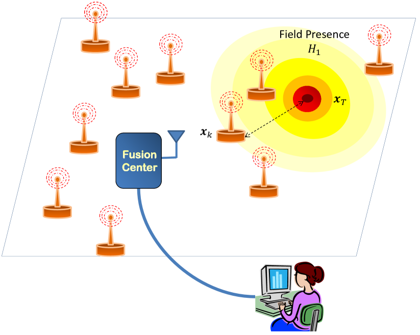
Unfortunately, the local detection probability is seldom known or difficult to estimate when the detection event relates to revealing a target described by a spatial signature. In fact, in the latter case the detection probability depends on the (unknown) constitutive parameters of the target to be detected, such as the average power and the target location (see Fig. 1.1). Without the knowledge of the local detection probabilities, the optimal fusion rule becomes impractical and an attractive alternative is the so-called Counting Rule (CR) test, i.e. the FC counts the number of local detections in the WSN and compares it with a threshold [13]. A performance analysis of the CR has been provided in [14] for a WSN with randomly deployed sensors. Unfortunately, CR suffers from performance degradation when trying to detect spatial events. Indeed, though CR is a very reasonable approach arising from different rationales [4, 7, 8], it does not make any attempt to use information about the contiguity of sensors that declare (potential) target presence. Therefore, based on these considerations, several studies have focused on design of fusion rules filling the performance gap between the CV rule and the CR.

In [15] a two-step decision-fusion algorithm is proposed, in which sensors first correct their decisions on the basis of neighboring sensors, and then make a collective decision as a network. It is shown that in many situations relevant to random sensor field detection, the local vote correction achieves significantly higher target detection probability than decision fusion based on the CR. Also, for the proposed approach, an explicit formula for FC threshold choice (viz. false-alarm rate determination) was provided, based on normal approximation of the statistic under the target-absent hypothesis. A simple and more accurate alternative for threshold choice based on the beta-binomial approximation is proposed in [16]. In [17] the Generalized Likelihood Ratio Test (GLRT) for the distributed detection of a target with a deterministic Amplitude Attenuation Function (AAF) and known emitted power is developed, and its superiority is shown in comparison to the CR. It is worth noticing that a similar model assuming a deterministic AAF was employed to analyze the (approximate) theoretical performance of CR in [14]. Differently, a stochastic AAF (subsuming the Rayleigh fading model) is assumed in [18] and [19], the latter being able to account for possible amplitude fluctuations. In the same works, also a scan statistic and Bayesian-originated approaches were obtained and compared with existing alternatives. In both works, the average emitted power of the target is however assumed known.

However, in many cases it is of practical importance to assume that also the (average) target emitted power is not available at the FC, which well fits the case of an uncooperative target, i.e. there is no preliminary agreement between target and sensors in order to exchange the information related to the (average) emitted power or make it possible to be estimated. Examples of practical interest for an uncooperative target are the primary user in a cognitive-radio system or an oil-spill source measured by an underwater sensor network. To the best of authors’ knowledge, a few works have dealt with the latter case. In [20], a GLRT was derived for the case of unknown target position and emitted power and compared to the CR, the CV rule and a GLRT based on the awareness of target emitted power. It has been shown that the loss incurred by the proposed GLRT is marginal when compared to the “power-clairvoyant” GLRT. Differently, in [21] an asymptotic locally-optimum detector was obtained for a WSN with (random) sensors positions following a Poisson point process. Remarkably, the aforementioned study accounted for unknown emitted power. Unfortunately, the deterministic AAF there employed implicitly assumed that FC has available the target position, thus limiting its applicability, though some numerical analysis to investigate mismatched AAF performance was provided.

Figure 1.1: Distributed detection of a non-cooperative target with spatial signature: System model.

1.2 Summary of Contributions

In this paper, we focus on decentralized detection of a non-cooperative target with a spatially-dependent emission (signature). We consider the practical setup in which the received signal at each individual sensor is embedded in white Gaussian noise and affected by Rayleigh fading, with an AAF depending on the sensor-target distance (viz. stochastic AAF). The Rayleigh fading assumption is employed here to account for fluctuations of the transmitted signal due to multipath propagation. For energy- and bandwidth-efficiency purposes, each sensor performs a local decision on the absence/presence of the target and forwards it to a FC, which is in charge of providing a more accurate global decision. With reference to this setup, the main contributions of the present work can be summarized as follows:

• We first review the scenario where the emitted power is available (thus the sole target position is unknown) at the FC, in order to understand the basics of the problem under investigation and list various alternatives employed in the open literature, such as GLRT [17] and Bayesian approaches. Then we switch to the more realistic case of unknown target location and power, which is typical in surveillance tasks. In this context we provide a systematic analysis of several detectors based on: ($i)$ GLRT [20], ($ii$) Bayesian approach and ($iii$) hybrid combinations of the two (for sake of completeness).

• In order to reduce the computational complexity required by these approaches, we also develop two novel sub-optimal fusion rules based on the locally-optimum detection framework [22]. The first relies on Bayesian assumption for the sole target position, whereas the latter obviates the problem by resorting to Davies rationale [23]. The design and the analysis of such practical rules and their comparison to the aforementioned alternatives represents the main contribution of this work. We underline that, since a uniformly most powerful test does not exist for our problem (because of the unknown parameters), nothing can be said in advance on their relative performance. All the aforementioned detectors are also compared in terms of computational complexity;

• The scenario at hand is then extended to the demanding case of imperfect reporting channels (typical for battery-powered sensors implementing low-energy communications), modeled as Binary Symmetric Channels (BSCs). The proposed fusion rules are then extended to take into account the (additional) reporting uncertainty, under the assumption of known Bit-Error Probabilities (BEPs).

• Finally, simulation results are provided to compare all the considered rules in some practical scenarios and to underline the relevant trends.

1.3 Paper Organization and Manuscript Notation

The remainder of the paper is organized as follows: in Sec. 2 we describe the system model, with reference to local sensing and FC modeling. In Sec. 3.1 we recall and discuss the problem of distributed detection under the assumption of a known average target emitted power. Differently, Sec. 3.2 is devoted to the development of fusion rules which deal with the additional uncertainty of unknown power. Then, in Sec. 3.3 we extend the obtained fusion rules to the more general case of imperfect reporting channels between the sensors and the FC. All the considered rules are compared in terms of complexity in Sec. 3.4. Furthermore, in Sec. 4 a set of simulations is provided to compare the developed rules and assess the loss incurred by non-availability of emitted power. Finally, some conclusions are drawn in Sec. 5. Proofs and derivations are confined to a dedicated Appendix.

Notation - Lower-case bold letters denote vectors, with $a_{n}$ being the $n$th element of $\bm{a}$; upper-case calligraphic letters, e.g. $\mathcal{A}$, denote finite sets; $\mathbb{E}\{\cdot\}$, $\mathrm{var\{\cdot\}}$, $(\cdot)^{T}$, and $\left\|\cdot\right\|$ denote expectation, variance, transpose and Euclidean norm operators, respectively; $P(\cdot)$ and $p(\cdot)$ denote probability mass functions (pmfs) and probability density functions (pdfs), while $P(\cdot|\cdot)$ and $p(\cdot|\cdot)$ their corresponding conditional counterparts; $\mathcal{N}(\mu,\sigma^{2})$ denotes a Gaussian pdf with mean $\mu$ and variance $\sigma^{2}$; $\mathcal{Q}(\cdot)$ is the complementary cumulative distribution function (ccdf) of a standard normal random variable; finally the symbols $\propto$ and $\sim$ mean “statistically equivalent to” and “distributed as”, respectively.

2 System Model

We consider a scenario where $K$ sensors are deployed in a surveillance area to monitor the absence ($\mathcal{H}_{0}$) or presence ($\mathcal{H}_{1}$) of a target of interest having a spatial signature. The measurement model of the generic sensor is described in Sec. 2.1. Then, we introduce the local decision procedure employed (independently) by each sensor in Sec. 2.2. Finally, in Sec. 2.3 we describe the problem of fusing sensors decisions at the FC.

2.1 Sensing Model

When the target is present in the surveillance area (i.e. $\mathcal{H}_{1}$), we assume that its radiated signal is isotropic and experiences (distance-depending) path-loss, Rayleigh fading, and Additive White Gaussian Noise (AWGN), before reaching individual sensors. In other terms, the sensing model for $k$th sensor ($k\in\{1,\ldots,K\}$) under $\mathcal{H}_{1}$ is [19]

$$y_{k}=\xi_{k}\,g(\bm{x}_{T},\bm{x}_{k})+w_{k}\,,$$ (2.1)

where $y_{k}\in\mathbb{R}$ is signal measured by $k$th sensor and $w_{k}\sim\mathcal{N}(0,\sigma_{w,k}^{2})$ denotes the corresponding measurement noise. Furthermore, $\bm{x}_{T}\in\mathbb{R}^{d}$ denotes the unknown position of the target (in $d$-dimensional coordinates), while $\bm{x}_{k}\in\mathbb{R}^{d}$ denotes the known $k$th sensor position (in $d$-dimensional coordinates). The positions $\bm{x}_{T}$ and $\bm{x}_{k}$ uniquely determine the value of $g(\bm{x}_{T},\bm{x}_{k})$, generically denoting the AAF. Finally $\xi_{k}$ is a Gaussian distributed random variable, $\xi_{k}\sim\mathcal{N}(0,\sigma_{s}^{2})$, modelling fluctuations in the received signal strength at $k$th sensor. Due to spatial separation of the sensors, we assume that the noise contributions $w_{k}$s and the fading coefficients $\xi_{k}$s are both statistically independent. Depending on the peculiar scenario being investigated, $\sigma_{s}^{2}$ will be assumed either known (Sec. 3.1) or unknown (Sec. 3.2).

Then, the measured signal $y_{k}$ is distributed under hypotheses $\mathcal{H}_{0}$ and $\mathcal{H}_{1}$ as

$$y_{k}\,|\,\mathcal{H}_{0}\sim\mathcal{N}(0,\sigma_{w,k}^{2}),\qquad\quad y_{k}\,|\,\mathcal{H}_{1}\sim\mathcal{N}\left(0,\,\sigma_{s}^{2}\,g^{2}(\bm{x}_{T},\bm{x}_{k})+\sigma_{w,k}^{2}\right),$$ (2.2)

respectively. With reference to the specific AAF, two common examples [15, 19] are the power-law attenuated model

$$g(\bm{x}_{T},\bm{x}_{k})\triangleq\frac{1}{\sqrt{1+\left(\frac{\left\|\bm{x}_{T}-\bm{x}_{k}\right\|}{\eta}\right)^{\alpha}}}\,,$$ (2.3)

and the exponentially attenuated model

$$g(\bm{x}_{T},\bm{x}_{k})\triangleq\sqrt{\exp\left(-\frac{\left\|\bm{x}_{T}-\bm{x}_{k}\right\|^{2}}{\eta^{2}}\right)}\,.$$ (2.4)

In Eqs. (2.3) and (2.4) the parameter $\eta$ controls the (approximate) spatial signature extent produced by both AAFs, while $\alpha$ is a positive coefficient that dictates the rapidity of signal decay as a function of the distance in the case of power-law AAF.

Figure 2.1: Detection probability ($P_{d,k}$) field, for a fixed $P_{f,k}=0.05$: Power-law AAF. Top plot shows $P_{d,k}$ vs. $\bm{x}$ (generic sensor position) for a target located at $\bm{x}_{T}=[0.1\;0.5]^{T}$; bottom plot depicts $P_{d,k}$ vs. $\left\|\bm{x}_{T}-\bm{x}\right\|$.

Figure 2.2: Detection probability ($P_{d,k}$) field, for a fixed $P_{f,k}=0.05$: Exponential AAF. Top plot shows $P_{d,k}$ vs. $\bm{x}$ (generic sensor position) for a target located at $\bm{x}_{T}=[0.1\;0.5]^{T}$; bottom plot depicts $P_{d,k}$ vs. $\left\|\bm{x}_{T}-\bm{x}\right\|$.

2.2 Local Decision Approach

We assume that sensors make their local decisions individually without collaboration. Then, each sensor is faced to tackle the following composite hypothesis testing:

$$\begin{cases}\mathcal{H}_{0}\,:\,&y_{k}=w_{k}\\ \mathcal{H}_{1}\,:\,&y_{k}=\xi_{k}\,g(\bm{x}_{T},\bm{x}_{k})+w_{k}\end{cases}$$ (2.5)

Indeed, although the sensor may be aware of its own position $\bm{x}_{k}$, the target position $\bm{x}_{T}$ is clearly unknown, independently from the availability of the average emitted power $\sigma_{s}^{2}$. Nonetheless, for this specific sensing model it can be shown that this difficulty can be elegantly circumvented. To this end, we consider a local decision procedure based on the well-known Neyman-Pearson lemma [12]. More specifically, we consider the local Log Likelihood-Ratio (LLR) of $k$th sensor, denoted with $\lambda_{k}$, whose explicit expression is:

$$\lambda_{k} \triangleq\ln\left[\frac{p(y_{k}|\mathcal{H}_{1})}{p(y_{k}|\mathcal{H}_{0})}\right]$$

$$=\frac{1}{2}\ln\left[\frac{\sigma_{w,k}^{2}}{\sigma_{w,k}^{2}+\sigma_{s}^{2}\,g^{2}(\bm{x}_{T},\bm{x}_{k})}\right]+\frac{\sigma_{s}^{2}\,g^{2}(\bm{x}_{T},\bm{x}_{k})}{\sigma_{w,k}^{2}\left[\sigma_{w,k}^{2}+\sigma_{s}^{2}\,g^{2}(\bm{x}_{T},\bm{x}_{k})\right]}\,y_{k}^{2}\,,$$ (2.6)

Last equation reveals that the LLR is an increasing function of $y_{k}^{2}$, irrespective of the target average emitted power $\sigma_{s}^{2}$ and the target location $\bm{x}_{T}$. Therefore, by Karlin-Rubin theorem [24], the following energy test

$$y_{k}^{2}\begin{array}[]{c}{\scriptstyle\hat{\mathcal{H}}=\mathcal{H}}_{1}\\ \gtrless\\ {\scriptstyle\hat{\mathcal{H}}=\mathcal{H}}_{0}\end{array}\gamma_{k}\,$$ (2.7)

is Uniformly Most Powerful (UMP) in a local sense. Also, $\gamma_{k}$ is a suitable threshold chosen to ensure a certain false-alarm rate at the sensor (in Neyman-Pearson approach) or to minimize the error-probability (in the Bayesian framework). In view of the aforementioned considerations, in what follows we will assume that each sensor implements its local UMP test based on its (local) measurement $y_{k}$.

Furthermore, we observe that the performance of the energy test in Eq. (2.7) is easily obtained explicitly, in terms of the detection ($P_{d,k}\triangleq\Pr\{\lambda_{k}\geq\gamma_{k}|\mathcal{H}_{1}\}$) and false-alarm ($P_{f,k}\triangleq\Pr\{\lambda_{k}\geq\gamma_{k}|\mathcal{H}_{0}\}$) probabilities as [12]

$$P_{d,k} =2\,\mathcal{Q}\left(\sqrt{\frac{\gamma_{k}}{\sigma_{w,k}^{2}+\sigma_{s}^{2}\,g^{2}(\bm{x}_{T},\bm{x}_{k})}}\right);\qquad P_{f,k}=2\,\mathcal{Q}\left(\sqrt{\frac{\gamma_{k}}{\sigma_{w,k}^{2}}}\right).$$ (2.8)

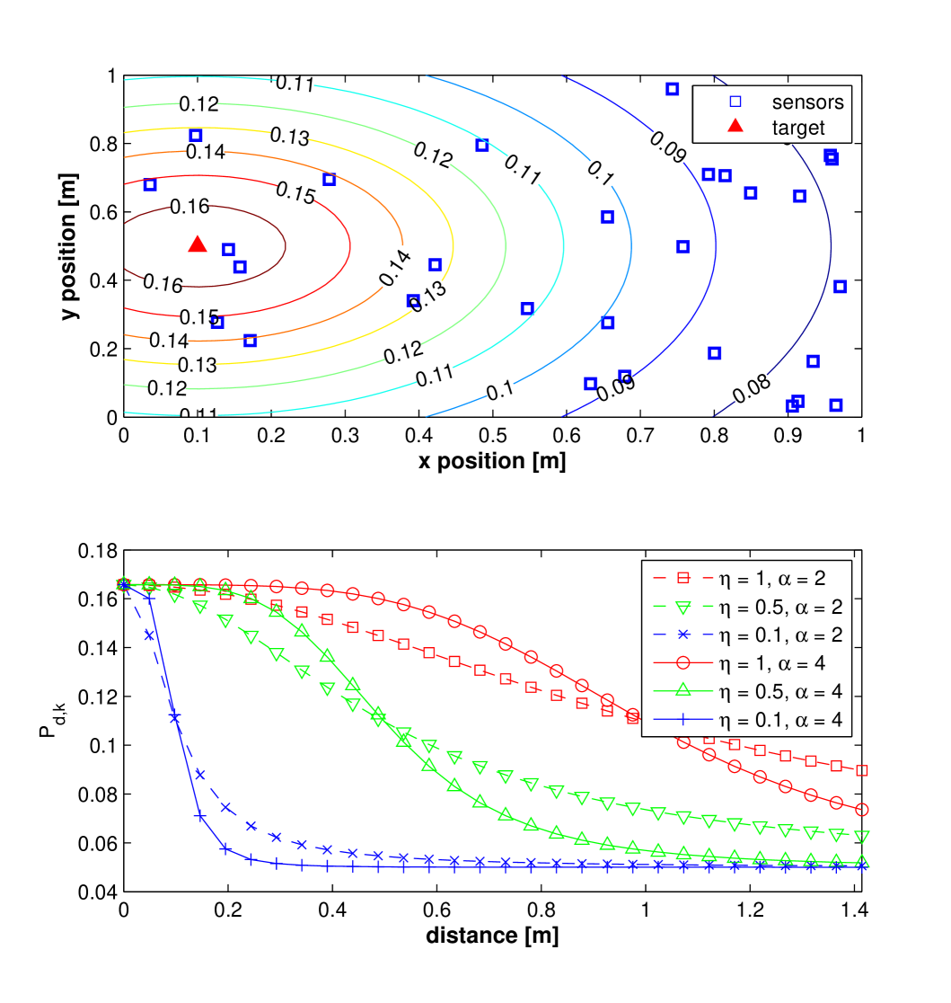
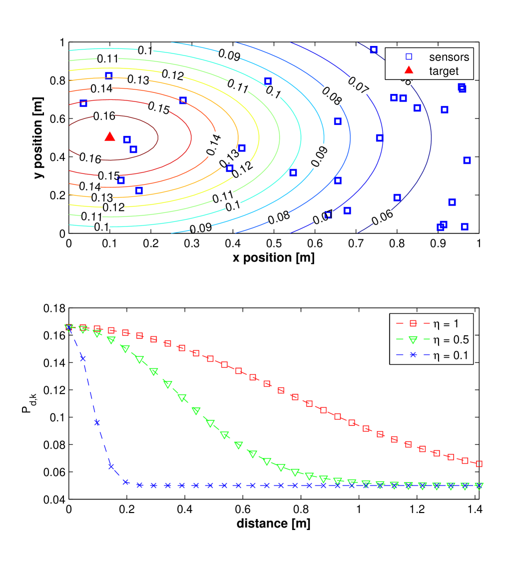
Two examples of a $P_{d,k}$ field (that is, the detection probability vs. the generic sensor position $\bm{x}$ for fixed target position and false-alarm probability) are depicted in the top plots of Figs. 2.1 and 2.2, for the power-law and exponential AAFs, respectively, with reference to a 2-D square surveillance area of length $L=1$. Also, we assumed $\bm{x}_{T}=\begin{bmatrix}0.1&0.5\end{bmatrix}^{T}$, $\eta=0.5$, $\alpha=2$, $\sigma_{w,k}^{2}=1$, $\sigma_{s}^{2}=1$ and $P_{f,k}=0.05$ (from which $\gamma_{k}$ is easily deduced, cf. Eq. (2.8)). Similarly, in the bottom plots of Figs. 2.1 and 2.2, we have showed the same $P_{d,k}$ (with the same parameters as the top plots) as a function of the distance $\left\|\bm{x}_{T}-\bm{x}\right\|$ for different values of $\eta\in\{0.1,0.5,1\}$ and $\alpha\in\{2,4\}$ (in the case of power law AAF).

Without loss of generality, we assume that $k$th sensor decision, denoted as $d_{k}$, follows the map $d_{k}=i$ when hypothesis $\mathcal{H}_{i}$ is declared. Finally, for the sake of notational compactness, we define the vector $\bm{d}\triangleq\begin{bmatrix}d_{1}&\cdots&d_{K}\end{bmatrix}^{T}$.

2.3 Decision Fusion

Each sensor then sends its decision $d_{k}$ to the FC, which employs a threshold-based decision test (we interchangeably use the term “fusion rule”) on the basis of vector $\bm{d}$, that is:

$$\Lambda(\bm{d})\begin{array}[]{c}{\scriptstyle\hat{\mathcal{H}}=\mathcal{H}}_{1}\\ \gtrless\\ {\scriptstyle\hat{\mathcal{H}}=\mathcal{H}}_{0}\end{array}\bar{\gamma}\,,$$ (2.9)

where $\bar{\gamma}$ is the threshold chosen to ensure a certain global false-alarm rate at the sensor (in Neyman-Pearson approach) or to minimize the global fusion error-probability (in the Bayesian framework) [12]. Global performance are accordingly evaluated in terms of (global) probability of false alarm ($P_{f,0}$ ) and detection ($P_{d,0}$), defined as follows

$$P_{f,0}\triangleq\Pr(\Lambda>\bar{\gamma}|\mathcal{H}_{0}),\qquad P_{d,0}\triangleq\Pr(\Lambda>\bar{\gamma}|\mathcal{H}_{1})\,.$$ (2.10)

It is worth noticing that $\Pr(\Lambda>\bar{\gamma}|\mathcal{H}_{i})$ generically describes both $P_{f,0}$ and $P_{d,0}$ (with $i=0$ and $i=1$, respectively). The behavior of the global probability of detection ($P_{d,0}$) versus the global probability of false alarm ($P_{f,0}$) is commonly denoted Receiver Operating Characteristic (ROC) [4].

It is apparent that, under hypothesis $\mathcal{H}_{1}$, the pmf of $\bm{d}$ assumes the explicit expression represented by the product of independent Bernoulli pmfs (since the decisions $d_{k}$ are conditionally independent, as an immediate consequence of mutual independence of $w_{k}$s, $\xi_{k}$s and of decoupled quantization process), that is

$$P(\bm{d}|\mathcal{H}_{1})=\prod_{k=1}^{K}P(d_{k}|\mathcal{H}_{1})=\prod_{k=1}^{K}(P_{d,k})^{d_{k}}(1-P_{d,k})^{(1-d_{k})}\,,$$ (2.11)

and a similar expression holds for $P(\bm{d}|\mathcal{H}_{0})$, when replacing $P_{d,k}$ with $P_{f,k}$. The optimal decision statistic in both Neyman-Pearson and Bayesian senses is represented by the (global) LLR, given by

$$\Lambda_{{\scriptscriptstyle\mathrm{LLR}}} \triangleq\ln\left[\frac{P(\bm{d}|\mathcal{H}_{1})}{P(\bm{d}|\mathcal{H}_{0})}\right]=\sum_{k=1}^{K}\ln\left[\frac{P(d_{k}|\mathcal{H}_{1})}{P(d_{k}|\mathcal{H}_{0})}\right]$$

$$=\sum_{k=1}^{K}\left\{d_{k}\ln\left[\frac{P_{d,k}}{P_{f,k}}\right]+(1-d_{k})\ln\left[\frac{1-P_{d,k}}{1-P_{f,k}}\right]\right\}\,,$$ (2.12)

where $P_{d,k}$ and $P_{f,k}$ are defined in Eq. (2.8). Unfortunately, the LLR cannot be implemented as the $P_{d,k}$s are usually unknown, since they depend on the constitutive parameters of the (unknown) target emission, that is ($i$) the average power $\sigma_{s}^{2}$ and ($ii$) the target location $\bm{x}_{T}$. Therefore, it is apparent that Eq. (2.12) should not be intended as a realistic element of comparison, but rather as an optimistic (upper) bound on the achievable performance, based on a clairvoyant assumption.

On the other hand, from direct inspection of Eq. (2.8), we notice that $P_{d,k}\geq P_{f,k}$ $\forall k\in\mathcal{K}$, as each reasonable local decision procedure would achieve a ROC — operation point that is more informative than an unbiased coin (i.e. above the chance line). Based on this observation, we may apply the well-known Counting Rule (CR) [4], not requiring sensors local performance for its implementation. This rule is widely used in DF (due to its simplicity and no requirements on system knowledge) and based on the following statistic:

$$\Lambda_{{\scriptscriptstyle\mathrm{CR}}}\triangleq\sum_{k=1}^{K}d_{k}\,.$$ (2.13)

The above rule, despite of its simplicity, has been obtained under different rationales in the literature [4, 7, 8]. In fact, Eq. (2.13) can be obtained as follows:

• It is statistically equivalent to the LLR in Eq. (2.12), by assuming that the sensors have all equal performance (i.e., $P_{d,k}=P_{d}$ and $P_{f,k}=P_{f}$) [4];

• It is statistically equivalent to the locally most-mean powerful test [25] in a partially-homogeneous scenario ($P_{f,k}=P_{f}$), assuming no other constraint than $P_{d,k}\geq P_{f,k}$ [8];

• It is the UMP invariant test for the permutation group [8];

• It is statistically equivalent to the GLRT and Rao test in a partially-homogeneous scenario ($P_{f,k}=P_{f}$, when $P_{f}<\frac{1}{2}$), assuming no other constraint than $P_{d,k}\geq P_{f,k}$ [8].

3 Practical Fusion Rules

3.1 Known Target Power

Initially, we assume that $\sigma_{s}^{2}$ is known and then the hypothesis testing problem can be summarized as:

$$\begin{cases}\mathcal{H}_{0}\,:\,&\sigma_{s}^{2}=0\\ \mathcal{H}_{1}\,:\,&\sigma_{s}^{2}>0\,(\mathrm{known})\,,\quad\bm{x}_{T}\,(\mathrm{nuisance})\end{cases},$$ (3.1)

that is, we are concerned with discriminating between two hypotheses where the nuisance parameters ($\bm{x}_{T}$) are present only under the (alternative) hypothesis $\mathcal{H}_{1}$. Such case has been analyzed in the works [13, 19].

GLRT

In [17] the authors proposed the use of a GLR statistic, whose explicit log form for the considered problem is

$$\Lambda_{\mathrm{G}} \triangleq\ln\left[\frac{\max_{\bm{x}_{T}}P(\bm{d}|\mathcal{H}_{1};\bm{x}_{T})}{P(\bm{d}|\mathcal{H}_{0})}\right]$$ (3.2)

$$=\sum_{k=1}^{K}\left\{d_{k}\,\ln\left[\frac{P_{d,k}(\widehat{\bm{x}}_{T})}{P_{f,k}}\right]+(1-d_{k})\,\ln\left[\frac{1-P_{d,k}(\widehat{\bm{x}}_{T})}{1-P_{f,k}}\right]\right\}\,,$$ (3.3)

where $\widehat{\bm{x}}_{T}$ denotes the Maximum Likelihood Estimate (MLE) of the target position, assuming that $\mathcal{H}_{1}$ holds, that is:

$$\widehat{\bm{x}}_{T}\triangleq\arg\max_{\bm{x}_{T}}\,P(\bm{d}|\mathcal{H}_{1};\bm{x}_{T})\,.$$ (3.4)

Clearly, the higher the estimation accuracy of $\bm{x}_{T}$, the higher the performance of GLR statistic. It is worth noticing that $\widehat{\bm{x}}_{T}$ cannot be obtained in closed form and therefore a grid search (or optimization routines) should be devised (details on implementation are later provided in Sec. 3.4). Exploiting the parametric independence of $P(\bm{d}|\mathcal{H}_{0})$ on $\bm{x}_{T}$ and the monotonic property of logarithm, the above expression can be rewritten in terms of Eq. (2.12) as:

$$\Lambda_{\mathrm{G}}=\max_{\bm{x}_{T}}\,\Lambda_{{\scriptscriptstyle\mathrm{LLR}}}(\bm{x}_{T})\,,$$ (3.5)

where $\Lambda_{{\scriptscriptstyle\mathrm{LLR}}}(\bm{x}_{T})$ underlines the evaluation of LLR in Eq. (2.12) assuming that the target position equals $\bm{x}_{T}$. The alternative form in (3.5) will be exploited to draw out interesting considerations when comparing GLRT with other detectors.

Bayesian Approach

The pdf dependence on target’s position under $\mathcal{H}_{1}$ may be eliminated if a prior distribution on the position itself is available (or can be safely assumed) and integrating the corresponding likelihood (see, for example, [26] for the advantages provided by the Bayesian approach). Then, the explicit expression of the Bayesian LLR is given by [19]

$$\Lambda_{\mathrm{B}} \triangleq\ln\left[\frac{\int P(\bm{d}|\mathcal{H}_{1};\bm{x}_{T})\,p(\bm{x}_{T})d\bm{x}_{T}}{P(\bm{d}|\mathcal{H}_{0})}\right]$$

$$=\ln\int\prod_{k=1}^{K}\left(\frac{P_{d,k}(\bm{x}_{T})}{P_{f,k}}\right)^{d_{k}}\left(\frac{1-P_{d,k}(\bm{x}_{T})}{1-P_{f,k}}\right)^{(1-d_{k})}\,p(\bm{x}_{T})\,d\bm{x}_{T}\,,$$ (3.6)

where the dependence of $P_{d,k}$ on target position $\bm{x}_{T}$ is underlined. It is interesting to notice that the above expression can be rewritten as:

$$\Lambda_{\mathrm{B}}=\ln\int\exp\left(\Lambda_{{\scriptscriptstyle\mathrm{LLR}}}(\bm{x}_{T})\right)\,p(\bm{x}_{T})\,d\bm{x}_{T}\,,$$ (3.7)

where $\Lambda_{{\scriptscriptstyle\mathrm{LLR}}}(\bm{x}_{T})$ has an analogous definition as that in Eq. (3.5).

3.2 Unknown Target Power

Differently, when $\sigma_{s}^{2}$ is assumed unknown, the resulting (composite) hypothesis testing generalizes to:

$$\begin{cases}\mathcal{H}_{0}\,:\,&\sigma_{s}^{2}=0\\ \mathcal{H}_{1}\,:\,&\sigma_{s}^{2}>0\,,\quad\bm{x}_{T}\,(\mathrm{nuisance})\end{cases}$$ (3.8)

The above problem is recognized as a one-sided hypothesis testing with nuisance parameters that are present only under the (alternative) hypothesis $\mathcal{H}_{1}$. In the rest of the paper, for the sake of notational convenience, we will use the symbol $\theta$ to refer to the unknown average power $\sigma_{s}^{2}$ (with corresponding notation $\theta_{0}$ for $\sigma_{s}^{2}=0$).

Discussion: Counting Rule (CR) and Clairvoyant LLR

It is worth noticing that, in the case of unknown power $\sigma_{s}^{2}$, the CR can be still implemented, as it does not require the knowledge of the $P_{d,k}$s (cf. Eq. (2.13)). Similarly, in the present scenario we will refer to the statistic which has (unrealistic) knowledge of both $\bm{x}_{T}$ and $\sigma_{s}^{2}$ as a clairvoyant LLR and thus the same formula as in Eq. (2.12) can be applied. Apparently, in the considered scenario, the LLR will represent an even looser benchmark on the performance of practical fusion rules.

GLRT

The GLRT for this case was proposed and analyzed in [20]. Indeed, the explicit expression of the (log-)GLR statistic is:

$$\Lambda_{\mathrm{G}} \triangleq\ln\left[\frac{\max_{\sigma_{s}^{2},\bm{x}_{T}}P(\bm{d}|\mathcal{H}_{1};\bm{x}_{T},\sigma_{s}^{2})}{P(\bm{d}|\mathcal{H}_{0})}\right]$$ (3.9)

$$=\sum_{k=1}^{K}\left\{d_{k}\,\ln\left[\frac{P_{d,k}\left(\widehat{\bm{x}}_{T},\widehat{\sigma_{s}^{2}}\right)}{P_{f,k}}\right]+(1-d_{k})\,\ln\left[\frac{1-P_{d,k}\left(\widehat{\bm{x}}_{T},\widehat{\sigma_{s}^{2}}\right)}{1-P_{f,k}}\right]\right\}\,,$$ (3.10)

where $\widehat{\bm{x}}_{T}$ and $\widehat{\sigma_{s}^{2}}$ denote the ML estimates of the target position and (average) target power, assuming that hypothesis $\mathcal{H}_{1}$ is true, that is:

$$\left(\widehat{\bm{x}}_{T},\widehat{\sigma_{s}^{2}}\right)\triangleq\arg\max_{\bm{x}_{T},\,\sigma_{s}^{2}}\,P(\bm{d}|\mathcal{H}_{1};\bm{x}_{T},\sigma_{s}^{2})\,.$$ (3.11)

The above expression can be rewritten (similarly as in the case of known power, cf. Eq. (3.5)) in terms of Eq. (2.12) as:

$$\Lambda_{\mathrm{G}}=\max_{\bm{x}_{T},\sigma_{s}^{2}}\,\Lambda_{{\scriptscriptstyle\mathrm{LLR}}}(\bm{x}_{T},\sigma_{s}^{2})\,,$$ (3.12)

where $\Lambda_{{\scriptscriptstyle\mathrm{LLR}}}(\bm{x}_{T},\sigma_{s}^{2})$ is used to denote the LLR of Eq. (2.12) evaluated assuming the target position and power corresponding to $\bm{x}_{T}$ and $\sigma_{s}^{2}$, respectively.

Bayesian Approach

In order to follow a purely Bayesian approach, we need eliminate both the dependence on target’s position and average emitted power (under $\mathcal{H}_{1}$) by assigning prior distributions to them both and integrating the corresponding likelihood. Thus, the closed form of the Bayesian LLR is given by [19]

$$\Lambda_{\mathrm{B}} \triangleq\ln\left[\frac{\int P(\bm{d}|\mathcal{H}_{1};\bm{x}_{T},\sigma_{s}^{2})\,p(\bm{x}_{T})\,p(\sigma_{s}^{2})\,d\bm{x}_{T}\,d\sigma_{s}^{2}}{P(\bm{d}|\mathcal{H}_{0})}\right]$$ (3.13)

$$=\ln\int\prod_{k=1}^{K}\left(\frac{P_{d,k}(\bm{x}_{T},\sigma_{s}^{2})}{P_{f,k}}\right)^{d_{k}}\left(\frac{1-P_{d,k}(\bm{x}_{T},\sigma_{s}^{2})}{1-P_{f,k}}\right)^{(1-d_{k})}\,p(\bm{x}_{T})\,p(\sigma_{s}^{2})\,d\bm{x}_{T}\,d\sigma_{s}^{2}\,.$$ (3.14)

As previously shown, the above expression can be similarly rewritten as:

$$\Lambda_{\mathrm{B}}=\ln\int\exp\left(\Lambda_{{\scriptscriptstyle\mathrm{LLR}}}(\bm{x}_{T},\sigma_{s}^{2})\right)\,p(\bm{x}_{T})\,p(\sigma_{s}^{2})\,d\bm{x}_{T}\,d\sigma_{s}^{2}\,,$$ (3.15)

where $\Lambda_{{\scriptscriptstyle\mathrm{LLR}}}(\bm{x}_{T},\sigma_{s}^{2})$ has an analogous definition as in Eq. (3.12).

Hybrid GLRT/Bayesian approaches

Other approaches can be obtained by mixing the two previous philosophies. For example, assuming a prior distribution to the target position and treating the average emitted power $\sigma_{s}^{2}$ as an unknown and deterministic parameter, leads to the following decision statistic:

$$\Lambda_{\mathrm{GB1}} \triangleq\ln\left[\frac{\max_{\sigma_{s}^{2}}\int P(\bm{d}|\mathcal{H}_{1};\bm{x}_{T},\sigma_{s}^{2})\,p(\bm{x}_{T})d\bm{x}_{T}}{P(\bm{d}|\mathcal{H}_{0})}\right]$$ (3.16)

$$=\ln\max_{\sigma_{s}^{2}}\left\{\int\prod_{k=1}^{K}\left(\frac{P_{d,k}(\bm{x}_{T},\sigma_{s}^{2})}{P_{f,k}}\right)^{d_{k}}\left(\frac{1-P_{d,k}(\bm{x}_{T},\sigma_{s}^{2})}{1-P_{f,k}}\right)^{(1-d_{k})}\,p(\bm{x}_{T})\,d\bm{x}_{T}\right\}\,.$$ (3.17)

The above statistic can be re-expressed as

$$\Lambda_{\mathrm{GB1}}=\max_{\sigma_{s}^{2}}\,\ln\int\exp(\Lambda_{{\scriptscriptstyle\mathrm{LLR}}}(\bm{x}_{T},\sigma_{s}^{2}))\,p(\bm{x}_{T})\,d\bm{x}_{T}\,,$$ (3.18)

with $\Lambda_{{\scriptscriptstyle\mathrm{LLR}}}(\bm{x}_{T},\sigma_{s}^{2})$ having the usual interpretation. Alternatively, we can pursue a dual approach, by assuming a prior distribution for $\sigma_{s}^{2}$ and treating the target position $\bm{x}_{T}$ as unknown and deterministic. In the latter case, the following decision statistic can be obtained:

$$\Lambda_{\mathrm{GB2}} \triangleq\ln\left[\frac{\max_{\bm{x}_{T}}\int P(\bm{d}|\mathcal{H}_{1};\bm{x}_{T},\sigma_{s}^{2})\,p(\sigma_{s}^{2})\,d\sigma_{s}^{2}}{P(\bm{d}|\mathcal{H}_{0})}\right]$$ (3.19)

$$=\ln\max_{\bm{x}_{T}}\left\{\int\prod_{k=1}^{K}\left(\frac{P_{d,k}(\bm{x}_{T},\sigma_{s}^{2})}{P_{f,k}}\right)^{d_{k}}\left(\frac{1-P_{d,k}(\bm{x}_{T},\sigma_{s}^{2})}{1-P_{f,k}}\right)^{(1-d_{k})}\,p(\sigma_{s}^{2})\,d\sigma_{s}^{2}\right\}\,.$$ (3.20)

The dual statistic can be similarly rewritten as

$$\Lambda_{\mathrm{GB2}}=\max_{\bm{x}_{T}}\,\ln\int\exp(\Lambda_{{\scriptscriptstyle\mathrm{LLR}}}(\bm{x}_{T},\sigma_{s}^{2}))\,p(\sigma_{s}^{2})\,d\sigma_{s}^{2}\,.$$ (3.21)

(Hybrid) Bayesian Locally-Optimum Detection Approach

In this case, we depart from naive Bayesian and GLRT approaches. More specifically, our aim is to exploit the one-sided nature (when referring to $\sigma_{s}^{2}$) of the hypothesis testing considered (cf. Eq. (3.8)). However, the problem here is complicated by the presence of the nuisance parameter $\bm{x}_{T}$ under the hypothesis $\mathcal{H}_{1}$. To this end, in order to get rid of the dependence on $\bm{x}_{T}$, we consider it as an unknown random parameter and assign a prior distribution $p(\bm{x}_{T})$. Then, we consider the averaged pdf under $\mathcal{H}_{1}$:

$$P(\bm{d}|\mathcal{H}_{1};\theta)=\int P(\bm{d}|\mathcal{H}_{1};\bm{x}_{T},\theta)\,p(\bm{x}_{T})\,d\bm{x}_{T}\,,$$ (3.22)

where we have used the common variable $\theta$ in the place of $\sigma_{s}^{2}$. Once we have averaged out the dependence on $\bm{x}_{T}$, we can apply the usual Locally-Optimum Detector (LOD), exploiting the one-sided problem [22]. Its implicit form is given by:

$$\Lambda_{{\scriptscriptstyle\mathrm{BLOD}}}\triangleq\frac{\left.\frac{\partial\ln\left[P(\bm{d}|\mathcal{H}_{1};\theta)\right]}{\partial\theta}\right|_{\theta=\theta_{0}}}{\sqrt{I(\theta_{0})}},$$ (3.23)

where $I(\theta_{0})$ represents the Fisher Information (FI) evaluated at $\theta_{0}$, that is:

$$I(\theta)\triangleq\mathbb{E}\left\{\left(\frac{\partial\ln\left[P(\bm{d}|\mathcal{H}_{1};\theta)\right]}{\partial\theta}\right)^{2}\right\}.$$ (3.24)

Evaluation of the terms contained in (3.23) provides the explicit form of $\Lambda_{\mathrm{{\scriptscriptstyle BLOD}}}$, shown hereinafter (the detailed derivation is given in the Appendix):

$$\Lambda_{{\scriptscriptstyle\mathrm{BLOD}}}=\frac{\sum_{k=1}^{K}\frac{d_{k}-P_{f,k}}{P_{f,k}\left(1-P_{f,k}\right)}p_{w}\left(\sqrt{\frac{\gamma_{k}}{\sigma_{w,k}^{2}}}\right)\frac{\sqrt{\gamma_{k}}}{\left(\sigma_{w,k}^{2}\right)^{3/2}}\,\int g^{2}(\bm{x}_{T},\bm{x}_{k})\,p(\bm{x}_{T})d\bm{x}_{T}}{\sqrt{\sum_{k=1}^{K}\frac{1}{P_{f,k}\left(1-P_{f,k}\right)}\,p_{w}^{2}\left(\sqrt{\frac{\gamma_{k}}{\sigma_{w,k}^{2}}}\right)\frac{\gamma_{k}}{\left(\sigma_{w,k}^{2}\right)^{3}}\left(\int g^{2}(\bm{x}_{T},\bm{x}_{k})\,p(\bm{x}_{T})\,d\bm{x}_{T}\right)^{2}}}\,.$$ (3.25)

The so-called “Bayesian-LOD” (or B-LOD) statistic can be also rewritten in a more compact form. To this end, we define the following quantities:

$$\nu_{k}(d_{k}) \triangleq\frac{d_{k}-P_{f,k}}{P_{f,k}(1-P_{f,k})}\,p_{w}\left(\sqrt{\frac{\gamma_{k}}{\sigma_{w,k}^{2}}}\right)\frac{\sqrt{\gamma_{k}}}{\left(\sigma_{w,k}^{2}\right)^{3/2}}\,,$$ (3.26)

$$\psi_{k} \triangleq\frac{1}{P_{f,k}(1-P_{f,k})}\,p_{w}^{2}\left(\sqrt{\frac{\gamma_{k}}{\sigma_{w,k}^{2}}}\right)\frac{\gamma_{k}}{\left(\sigma_{w,k}^{2}\right)^{3}}\,.$$ (3.27)

Exploiting Eqs. (3.26) and (3.27) into (3.25), we obtain the equivalent expression:

$$\Lambda_{{\scriptscriptstyle\mathrm{BLOD}}}=\frac{\sum_{k=1}^{K}\nu_{k}(d_{k})\,\int g^{2}(\bm{x}_{T},\bm{x}_{k})\,p(\bm{x}_{T})\,d\bm{x}_{T}}{\sqrt{\sum_{k=1}^{K}\psi_{k}\,\left(\int g^{2}(\bm{x}_{T},\bm{x}_{k})\,p(\bm{x}_{T})\,d\bm{x}_{T}\right)^{2}}}\,.$$ (3.28)

Generalized LOD based on Davies approach

A different approach to exploiting the one-sided nature of the problem under investigation consists in adopting the detection approach proposed by Davies [23]. The aforementioned approach allows to extend score-based tests to the case of nuisance parameters present under the sole $\mathcal{H}_{1}$, as these tests require the ML estimates of nuisances under $\mathcal{H}_{0}$ (which thus cannot be obtained). The building rationale of Davies approach is summarized as follows.

When $\bm{x}_{T}$ is known in (3.8), the problem reduces to a simple one-sided testing. In the latter case, the LOD seems a reasonable decision procedure for the problem. However, since in practice $\bm{x}_{T}$ is unknown, a family of statistics is rather obtained by varying $\bm{x}_{T}$. Hence, to overcome this technical difficulty, Davies proposed the use of the maximum of the family of the statistics, following a “GLRT-like” approach. In what follows, we will refer to the employed decision test as Generalized LOD (G-LOD), to underline the use of LOD as the inner statistic employed in Davies approach.

The implicit form of the G-LOD is given by [23]:

$$\Lambda_{{\scriptscriptstyle\mathrm{GLOD}}}\triangleq\max_{\bm{x}_{T}}\frac{\left.\frac{\partial\ln\left[P(\bm{d}|\mathcal{H}_{1};\bm{x}_{T},\theta)\right]}{\partial\theta}\right|_{\theta=\theta_{0}}}{\sqrt{I(\theta_{0},\bm{x}_{T})}},$$ (3.29)

where the symbol $I(\theta,\bm{x}_{T})$ is used to denote the FI assuming $\bm{x}_{T}$ known, that is:

$$I(\theta,\bm{x}_{T})\triangleq\mathbb{E}\left\{\left(\frac{\partial\ln\left[P(\bm{d}|\mathcal{H}_{1};\bm{x}_{T},\theta)\right]}{\partial\theta}\right)^{2}\right\}.$$ (3.30)

The derivation of the inner term in Eq. (3.29) is provided in Appendix. The explicit form is given as:

$$\Lambda_{{\scriptscriptstyle\mathrm{GLOD}}}=\max_{\bm{x}_{T}}\frac{\sum_{k=1}^{K}\frac{d_{k}-P_{f,k}}{P_{f,k}(1-P_{f,k})}\,p_{w}\left(\sqrt{\frac{\gamma_{k}}{\sigma_{w,k}^{2}}}\right)\frac{\sqrt{\gamma_{k}}\,g^{2}(\bm{x}_{T},\bm{x}_{k})}{\left(\sigma_{w,k}^{2}\right)^{3/2}}}{\sqrt{\sum_{k=1}^{K}\frac{1}{P_{f,k}(1-P_{f,k})}\,p_{w}^{2}\left(\sqrt{\frac{\gamma_{k}}{\sigma_{w,k}^{2}}}\right)\frac{\gamma_{k}\,g^{4}(\bm{x}_{T},\bm{x}_{k})}{\left(\sigma_{w,k}^{2}\right)^{3}}}}\,.$$ (3.31)

The G-LOD can be also expressed in the compact form

$$\Lambda_{{\scriptscriptstyle\mathrm{GLOD}}}=\max_{\bm{x}_{T}}\frac{\sum_{k=1}^{K}\nu_{k}(d_{k})\,g^{2}(\bm{x}_{T},\bm{x}_{k})}{\sqrt{\sum_{k=1}^{K}\psi_{k}\,g^{4}(\bm{x}_{T},\bm{x}_{k})}}\,,$$ (3.32)

by exploiting the same definitions as the B-LOD in Eqs. (3.26) and (3.27), respectively.

3.3 Imperfect Reporting Channels

The previous sections assumed that binary data $d_{k}$ from the WSN could be transmitted to the FC without any distortion. In this section, we consider an imperfect link scenario where the one-bit quantized data are sent to the FC over (independent) BSCs, in order to account for limited transmit energy and possible failures of the sensors. We observe that the BSC model arises when separation between sensing and communication layers is performed in the design phase (namely a “decode-then-fuse” approach [27, 28]).

More specifically, we assume that the FC observes a noisy binary-valued signal $\widehat{d}_{k}$ from $k$th sensor, that is:

$$\widehat{d}_{k}=\begin{cases}d_{k}&\mathrm{with}\,\mathrm{probability\;}(1-P_{e,k})\\ 1-d_{k}\quad&\mathrm{with}\,\mathrm{probability\;}P_{e,k}\end{cases}$$ (3.33)

Here $P_{e,k}$ denotes the BEP on the $k$th link. Throughout this paper we make the reasonable assumption $P_{e,k}\leq\frac{1}{2}$ and we hypothesize that $P_{e,k}$ values can be safely estimated by the FC (that is they are known). This is for example the case when coherent detection or non-coherent detection with orthogonal symbols is performed over a fading channel, as soon as the corresponding Signal-To-Noise Ratio (SNR) can be obtained, e.g. [7, 29, 30]. Then, we similarly collect the received (noisy) decisions as $\widehat{\bm{d}}\triangleq\left[\begin{array}[]{ccc}\widehat{d}_{1}&\cdots&\widehat{d}_{K}\end{array}\right]^{T}$.

It is apparent that, under hypothesis $\mathcal{H}_{1}$, the pmf of $\widehat{\bm{d}}$ still assumes a similar (to the noise-free reporting channels case) expression given by the product of independent Bernoulli pmfs (since the reporting channels are assumed to act independently), that is:

$$P(\widehat{\bm{d}}|\mathcal{H}_{1}) =\prod_{k=1}^{K}P(\widehat{d}_{k}|\mathcal{H}_{1})\,=\,\prod_{k=1}^{K}(\rho_{1,k})^{\widehat{d}_{k}}\,(1-\rho_{1,k})^{(1-\widehat{d}_{k})}\,,$$ (3.34)

where $\rho_{1,k}\triangleq\left[\left(1-P_{e,k}\right)P_{d,k}+P_{e,k}(1-P_{d,k})\right]$. Also, a similar expression holds for $P(\widehat{\bm{d}}|\mathcal{H}_{0})$, when replacing $\rho_{1,k}$ with $\rho_{0,k}\triangleq\left[\left(1-P_{e,k}\right)P_{f,k}+P_{e,k}(1-P_{f,k})\right]$. We remark that $P_{d,k}$ and $P_{f,k}$ retain the same definition of Eq. (2.8).

Discussion: Counting Rule (CR) and Clairvoyant LLR

First, it is worth noticing that, the CR rule can be still applied in the case of error-prone reporting channels, as long as $\rho_{1,k}\geq\rho_{0,k}$. Such condition is satisfied as long as the reasonable conditions $P_{d,k}\geq P_{f,k}$ and $P_{e,k}\leq 1/2$ hold, respectively. Secondly, the (clairvoyant) LLR is given by

$$\Lambda_{{\scriptscriptstyle\mathrm{LLR}}} \triangleq\ln\left[\frac{P(\widehat{\bm{d}}|\mathcal{H}_{1})}{P(\widehat{\bm{d}}|\mathcal{H}_{0})}\right]=\sum_{k=1}^{K}\ln\left[\frac{P(\widehat{d}_{k}|\mathcal{H}_{1})}{P(\widehat{d}_{k}|\mathcal{H}_{0})}\right]$$

$$=\sum_{k=1}^{K}\left\{\widehat{d}_{k}\ln\left[\frac{\rho_{1,k}}{\rho_{0,k}}\right]+(1-\widehat{d}_{k})\ln\left[\frac{1-\rho_{1,k}}{1-\rho_{0,k}}\right]\right\}\,.$$ (3.35)

As in the case of error-free reporting channels, the clairvoyant LLR requires knowledge of both $\bm{x}_{T}$ and $\sigma_{s}^{2}$ and additionally of BEPs $P_{e,k}$. Also, we recall that the additionally uncertainty arising from the BSCs should not affect the relative loss in performance incurred by the proposed rules in comparison to the LLR, as they will all rely on the availability of $P_{e,k}$. The sole exception is represented by the CR, which does not rely on $P_{e,k}$s for its implementation (it only requires $P_{e,k}\leq 1/2$).

GLRT

In the present scenario, the explicit expression of the (log-)GLR statistic generalizes to:

$$\Lambda_{\mathrm{G}}\triangleq \ln\left[\frac{\max_{\sigma_{s}^{2},\bm{x}_{T}}P(\widehat{\bm{d}}|\mathcal{H}_{1};\bm{x}_{T},\sigma_{s}^{2})}{P(\widehat{\bm{d}}|\mathcal{H}_{0})}\right]$$ (3.36)

$$= \sum_{k=1}^{K}\left\{\widehat{d}_{k}\,\ln\left[\frac{\rho_{1,k}\left(\widehat{\bm{x}}_{T},\widehat{\sigma_{s}^{2}}\right)}{\rho_{0,k}}\right]+(1-\widehat{d}_{k})\,\ln\left[\frac{1-\rho_{1,k}\left(\widehat{\bm{x}}_{T},\widehat{\sigma_{s}^{2}}\right)}{1-\rho_{0,k}}\right]\right\}\,,$$ (3.37)

where $\widehat{\bm{x}}_{T}$ and $\widehat{\sigma_{s}^{2}}$ denote the usual ML estimates of the target position and (average) emitted reference power, assuming that $\mathcal{H}_{1}$ is true. Also, we have adopted the notation $\rho_{1,k}(\bm{x}_{T},\sigma_{s}^{2})$ to underline the dependence on $\bm{x}_{T}$ and $\sigma_{s}^{2}$ via $P_{d,k}(\bm{x}_{T},\sigma_{s}^{2})$. Finally, we remark that the above expression can be similarly rewritten in terms of the clairvoyant LLR in (3.35) as Eq. (3.12).

Bayesian Approach

In the case of imperfect reporting channels, the explicit expression of the (purely) Bayesian LLR generalizes to:

$$\Lambda_{\mathrm{B}}\triangleq \ln\left[\frac{\int P(\widehat{\bm{d}}|\mathcal{H}_{1};\bm{x}_{T},\sigma_{s}^{2})\,p(\bm{x}_{T})\,p(\sigma_{s}^{2})\,d\bm{x}_{T}\,d\sigma_{s}^{2}}{P(\widehat{\bm{d}}|\mathcal{H}_{0})}\right]$$ (3.38)

$$= \ln\int\prod_{k=1}^{K}\left(\frac{\rho_{1,k}(\bm{x}_{T},\sigma_{s}^{2})}{\rho_{0,k}}\right)^{\widehat{d}_{k}}\times\left(\frac{1-\rho_{1,k}(\bm{x}_{T},\sigma_{s}^{2})}{1-\rho_{0,k}}\right)^{(1-\widehat{d}_{k})}p(\bm{x}_{T})\,p(\sigma_{s}^{2})\,d\bm{x}_{T}\,d\sigma_{s}^{2}\,.$$ (3.39)

As previously shown, the above expression can be similarly rewritten as in Eq. (3.15), exploiting the LLR definition provided in (3.35).

Hybrid GLRT/Bayesian approaches

Hybrid GLRT/Bayesian approaches are straightforwardly extended as follows. For example, assuming a prior for the target position $\bm{x}_{T}$ and treating $\sigma_{s}^{2}$ as deterministic provides:

$$\Lambda_{\mathrm{GB1}} \triangleq\ln\left[\frac{\max_{\sigma_{s}^{2}}\int P\left(\widehat{\bm{d}}|\mathcal{H}_{1};\bm{x}_{T},\sigma_{s}^{2}\right)\,p(\bm{x}_{T})d\bm{x}_{T}}{P\left(\widehat{\bm{d}}|\mathcal{H}_{0}\right)}\right]$$ (3.40)

$$=\ln\max_{\sigma_{s}^{2}}\int\left\{\prod_{k=1}^{K}\left(\frac{\rho_{1,k}(\bm{x}_{T},\sigma_{s}^{2})}{\rho_{0,k}}\right)^{\widehat{d}_{k}}\left(\frac{1-\rho_{1,k}(\bm{x}_{T},\sigma_{s}^{2})}{1-\rho_{0,k}}\right)^{(1-\widehat{d}_{k})}\right\}\,p(\bm{x}_{T})\,d\bm{x}_{T}$$ (3.41)

The above statistic can be re-expressed in terms of the LLR similarly as Eq. (3.18). Alternatively, assuming a prior distribution for $\sigma_{s}^{2}$ and treating the target position $\bm{x}_{T}$ as unknown deterministic, the complementary hybrid statistic generalizes to:

$$\Lambda_{\mathrm{GB2}}\triangleq \ln\left[\frac{\max_{\bm{x}_{T}}\int P\left(\widehat{\bm{d}}|\mathcal{H}_{1};\bm{x}_{T},\sigma_{s}^{2}\right)\,p(\sigma_{s}^{2})\,d\sigma_{s}^{2}}{P\left(\widehat{\bm{d}}|\mathcal{H}_{0}\right)}\right]$$ (3.42)

$$= \ln\max_{\bm{x}_{T}}\int\left\{\prod_{k=1}^{K}\left(\frac{\rho_{1,k}(\bm{x}_{T},\sigma_{s}^{2})}{\rho_{0,k}}\right)^{\widehat{d}_{k}}\left(\frac{1-\rho_{1,k}(\bm{x}_{T},\sigma_{s}^{2})}{1-\rho_{0,k}}\right)^{(1-\widehat{d}_{k})}\,p(\sigma_{s}^{2})\,d\sigma_{s}^{2}\right\}$$ (3.43)

As usual, the above statistic can be re-expressed in terms of LLR similarly as Eq. (3.21).

(Hybrid) Bayesian Locally-Optimum Detection Approach

To approach the detection problem through the common LOD approach, we first consider the averaged pdf under $\mathcal{H}_{1}$:

$$P\left(\widehat{\bm{d}}\,|\,\mathcal{H}_{1};\theta\right)=\int P\left(\widehat{\bm{d}}\,|\,\mathcal{H}_{1};\bm{x}_{T},\theta\right)\,p(\bm{x}_{T})\,d\bm{x}_{T}\,.$$ (3.44)

The implicit form of the LOD is thus given by:

$$\Lambda_{{\scriptscriptstyle\mathrm{BLOD}}}\triangleq\frac{\left.\frac{\partial\ln\left[P\left(\widehat{\bm{d}}\,|\,\mathcal{H}_{1};\theta\right)\right]}{\partial\theta}\right|_{\theta=\theta_{0}}}{\sqrt{I(\theta_{0})}},$$ (3.45)

where $I(\theta_{0})$ represents the usual FI evaluated at $\theta_{0}$, that is:

$$I(\theta)\triangleq\mathbb{E}\left\{\left(\frac{\partial\ln\left[P\left(\widehat{\bm{d}}\,|\,\mathcal{H}_{1};\theta\right)\right]}{\partial\theta}\right)^{2}\right\}.$$ (3.46)

The explicit form of $\Lambda_{\mathrm{{\scriptscriptstyle BLOD}}}$ is shown as follows (the derivation is left to the reader for the sake of brevity):

$$\Lambda_{{\scriptscriptstyle\mathrm{BLOD}}}=\frac{\sum_{k=1}^{K}\frac{\widehat{d}_{k}-\rho_{0,k}}{\rho_{0,k}\left(1-\rho_{0,k}\right)}\,(1-2P_{e,k})\,p_{w}\left(\sqrt{\frac{\gamma_{k}}{\sigma_{w,k}^{2}}}\right)\frac{\sqrt{\gamma_{k}}}{\left(\sigma_{w,k}^{2}\right)^{3/2}}\left(\int g^{2}(\bm{x}_{T},\bm{x}_{k})\,p(\bm{x}_{T})\,d\bm{x}_{T}\right)}{\sqrt{\sum_{k=1}^{K}\frac{1}{P_{f,k}\left(1-P_{f,k}\right)}\,p_{w}^{2}\left(\sqrt{\frac{\gamma_{k}}{\sigma_{w,k}^{2}}}\right)\frac{\gamma_{k}}{\left(\sigma_{w,k}^{2}\right)^{3}}\left(\int g^{2}(\bm{x}_{T},\bm{x}_{k})\,p(\bm{x}_{T})\,d\bm{x}_{T}\right)^{2}}}\,.$$ (3.47)

Similarly, by exploiting the following generalized definitions

$$\widehat{\nu}_{k}(\widehat{d}_{k}) \triangleq\frac{\widehat{d}_{k}-\rho_{0,k}}{\rho_{0,k}\left(1-\rho_{0,k}\right)}\,(1-2P_{e,k})\,p_{w}\left(\sqrt{\frac{\gamma_{k}}{\sigma_{w,k}^{2}}}\right)\frac{\sqrt{\gamma_{k}}}{\left(\sigma_{w,k}^{2}\right)^{3/2}}\,,$$ (3.48)

$$\widehat{\psi}_{k} \triangleq\frac{1}{\rho_{0,k}\left(1-\rho_{0,k}\right)}\,(1-2P_{e,k})^{2}\,p_{w}^{2}\left(\sqrt{\frac{\gamma_{k}}{\sigma_{w,k}^{2}}}\right)\frac{\gamma_{k}}{\left(\sigma_{w,k}^{2}\right)^{3}}\,,$$ (3.49)

the B-LOD can be also expressed in a similar compact form:

$$\Lambda_{{\scriptscriptstyle\mathrm{BLOD}}}=\frac{\sum_{k=1}^{K}\widehat{\nu}_{k}(\widehat{d}_{k})\,\int g^{2}(\bm{x}_{T},\bm{x}_{k})\,p(\bm{x}_{T})\,d\bm{x}_{T}}{\sqrt{\sum_{k=1}^{K}\widehat{\psi}_{k}\,\left(\int g^{2}(\bm{x}_{T},\bm{x}_{k})\,p(\bm{x}_{T})\,d\bm{x}_{T}\right)^{2}}}\,.$$ (3.50)

Generalized LOD based on Davies approach

The implicit form of LOD based on Davies approach is given by [23]:

$$\Lambda_{{\scriptscriptstyle\mathrm{GLOD}}}\triangleq\max_{\bm{x}_{T}}\frac{\left.\frac{\partial\ln\left[P\left(\widehat{\bm{d}}\,|\mathcal{H}_{1};\bm{x}_{T},\theta\right)\right]}{\partial\theta}\right|_{\theta=\theta_{0}}}{\sqrt{I(\bm{x}_{T},\theta_{0})}},$$ (3.51)

where the symbol $I(\bm{x}_{T},\theta)$ is used to denote the FI assuming $\bm{x}_{T}$ known, that is:

$$I(\bm{x}_{T},\theta)\triangleq\mathbb{E}\left\{\left(\frac{\partial\ln\left[P(\widehat{\bm{d}}|\mathcal{H}_{1};\bm{x}_{T},\theta)\right]}{\partial\theta}\right)^{2}\right\}.$$ (3.52)

The derivation of the inner term in Eq. (3.51) is left to the reader for sake of brevity. The explicit form is given as:

$$\Lambda_{{\scriptscriptstyle\mathrm{GLOD}}}=\max_{\bm{x}_{T}}\frac{\sum_{k=1}^{K}\frac{\widehat{d}_{k}-\rho_{0,k}}{\rho_{0,k}\left(1-\rho_{0,k}\right)}\,(1-2P_{e,k})\,p_{w}\left(\sqrt{\frac{\gamma_{k}}{\sigma_{w,k}^{2}}}\right)\frac{\sqrt{\gamma_{k}}\,g^{2}(\bm{x}_{T},\bm{x}_{k})}{\left(\sigma_{w,k}^{2}\right)^{3/2}}}{\sqrt{\sum_{k=1}^{K}\frac{(1-2P_{e,k})^{2}}{\rho_{0,k}\left(1-\rho_{0,k}\right)}\,p_{w}^{2}\left(\sqrt{\frac{\gamma_{k}}{\sigma_{w,k}^{2}}}\right)\frac{\gamma_{k}\,g^{4}(\bm{x}_{T},\bm{x}_{k})}{\left(\sigma_{w,k}^{2}\right)^{3}}}}\,.$$ (3.53)

Similarly, G-LOD can be also expressed in the compact form:

$$\Lambda_{{\scriptscriptstyle\mathrm{GLOD}}}=\max_{\bm{x}_{T}}\frac{\sum_{k=1}^{K}\widehat{\nu}_{k}(\widehat{d}_{k})\,g^{2}(\bm{x}_{T},\bm{x}_{k})}{\sqrt{\sum_{k=1}^{K}\widehat{\psi}_{k}\,\,g^{4}(\bm{x}_{T},\bm{x}_{k})}}\,,$$ (3.54)

by exploiting the same definitions as the B-LOD in Eqs. (3.48) and (3.49), respectively.

3.4 Summary of the Considered Rules and their Practical Implementation

In this section, we provide a summarizing comparison of the considered rules, focusing on the computational complexity (a performance comparison is then provided in Sec. 4). To this end, in Tab. 1 we report the explicit form of the considered fusion rules, as well as the corresponding complexity required for their implementation.

First of all, we observe that CR (cf. Eq. (2.13)) and B-LOD (cf. Eq. (3.50)) require the lowest complexity (that is $\mathcal{O}(K)$), as only a sum of $K$ terms needs to be evaluated (indeed the integrations of B-LOD in (3.50) can be performed off-line). Secondly, all the remaining rules require optimizations (GLRT and G-LOD), integrations (Bayesian approach) or both of them (viz. hybrid approaches). In this case, the complexity evaluation in Tab. 1 subsumes that a grid search or integration is performed, similarly as in [17, 19, 20]. Additionally, when dealing with prior pdfs, we employ non-informative priors with the intent of underlining useful analogies among proposed rules. Nonetheless, grid implementation (and corresponding complexity evaluation) still applies to the case of informative priors.

More specifically, after assuming that $\bm{x}_{T}$ and $\sigma_{s}^{2}$ belong to limited sets $\mathrm{S}_{\bm{x}_{T}}\subset\mathbb{R}^{d}$ and $S_{\mathrm{\sigma_{s}^{2}}}\subset\mathbb{R}^{+}$, respectively, the space ($\bm{x}_{T},\sigma_{s}^{2})$ is then discretized into:

• $N_{\bm{x}_{T}}$ position bins in the $d$-dimensional space, each one associated to a center bin position, say $\bm{x}_{T}[i]$, $i\in\{1,\ldots N_{\bm{x}_{T}}\}$;

• $N_{\sigma_{s}^{2}}$ variance (power) bins, each one to associated to a center bin variance, say $\sigma_{s}^{2}[j]$, $j\in\{1,\ldots N_{\sigma_{s}^{2}}\}$.

Grid implementation of GLRT: Starting from the alternative form of Eq. (3.12), we approximate the GLRT via the following grid search:

$$\Lambda_{\mathrm{G}}\approx\max_{i=1,\ldots N_{\bm{x}_{T}}}\,\max_{j=1,\ldots,N_{\sigma_{s}^{2}}}\,\Lambda_{{\scriptscriptstyle\mathrm{LLR}}}(\bm{x}_{T}[i]\,,\,\sigma_{s}^{2}[j])\,;$$ (3.55)

where we recall that $\Lambda_{{\scriptscriptstyle\mathrm{LLR}}}(\bm{x}_{T}[i]\,,\,\sigma_{s}^{2}[j])$ represents the expression of the clairvoyant LLR statistic obtained by evaluating the $P_{d,k}$s by replacing $\bm{x}_{T}$ and $\sigma_{s}^{2}$ with $\bm{x}_{T}[i]$ and $\sigma_{s}^{2}[j]$, respectively, into (2.8).

Grid implementation of Bayesian approach: First, we approximate the double integral in (3.15) through the Riemann sums as follows:

$$\Lambda_{\mathrm{B}} \approx\ln\left[\sum_{i=1}^{N_{\bm{x}_{T}}}\,\sum_{j=1}^{N_{\sigma_{s}^{2}}}\exp\left\{\Lambda_{{\scriptscriptstyle\mathrm{LLR}}}(\bm{x}_{T}[i],\sigma_{s}^{2}[j])+\ln\,r_{i}+\ln\,\bar{r}_{j}\right\}\right]\,,$$ (3.56)

where $r_{i}$ and $\bar{r}_{j}$ are the the mass probabilities associated to bins $i$ and $j$ of $\bm{x}_{T}$ and $\sigma_{s}^{2}$, through $p(\bm{x}_{T})$ and $p(\sigma_{s}^{2})$, respectively. In other words, $r_{i}\triangleq\Pr\{\bm{x}_{T}\in\mathcal{I}(\bm{x}_{T}[i])\}$ and $\bar{r}_{j}\triangleq\Pr\{\sigma_{s}^{2}\in\mathcal{I}(\sigma_{s}^{2}[j])\}$, where $\mathcal{I}(\bm{x}_{T}[i])$ and $\mathcal{I}(\sigma_{s}^{2}[j])$ denote the extent of $i$th and $j$th bins of the grid employed. This approximation admits a more intuitive form when the prior pdfs are assumed non-informative (viz. uniform). Indeed, in the latter case, the above approximation specializes into:

$$\Lambda_{\mathrm{B}} \approx r\,\bar{r}\,\ln\left[\sum_{i=1}^{N_{\bm{x}_{T}}}\,\sum_{j=1}^{N_{\sigma_{s}^{2}}}\,\exp(\Lambda_{{\scriptscriptstyle\mathrm{LLR}}}(\bm{x}_{T}[i],\sigma_{s}^{2}[j]))\right]\,,$$ (3.57)

$$\propto\ln\left[\sum_{i=1}^{N_{\bm{x}_{T}}}\,\sum_{j=1}^{N_{\sigma_{s}^{2}}}\,\exp(\Lambda_{{\scriptscriptstyle\mathrm{LLR}}}(\bm{x}_{T}[i],\sigma_{s}^{2}[j]))\right]\,.$$ (3.58)

The right-hand side is in the form of the well-known log-sum-exp combination, which can be also interpreted as a “soft-max” function. Therefore it is apparent that GLR approximation in (3.55) shows a clear connection with the Bayesian approach in (3.58), as also observed in [19] for the case of random sensor deployment.

Grid implementation of hybrid approaches: Remarkably, the hybrid fusion rules of Sec. 3.3 admit similar approximations as the pure GLR and Bayesian decision statistic. Indeed, $\Lambda_{\mathrm{GB1}}$ in (3.18) is approximated (assuming a uniform pdf for $p(\bm{x}_{T})$) as

$$\Lambda_{\mathrm{GB1}}\approx\max_{j=1,\ldots,N_{\sigma_{s}^{2}}}\,\ln\sum_{i=1}^{N_{\bm{x}_{T}}}\exp(\Lambda_{{\scriptscriptstyle\mathrm{LLR}}}(\bm{x}_{T}[i],\sigma_{s}^{2}[j]))\,,$$ (3.59)

while $\Lambda_{\mathrm{GB2}}$ in (3.21) is approximated (assuming a uniform pdf for $p(\sigma_{s}^{2})$) as:

$$\Lambda_{\mathrm{GB2}}\approx\max_{i=1,\ldots N_{\bm{x}_{T}}}\,\ln\sum_{j=1}^{N_{\sigma_{s}^{2}}}\exp(\Lambda_{{\scriptscriptstyle\mathrm{LLR}}}(\bm{x}_{T}[i],\sigma_{s}^{2}[j]))\,.$$ (3.60)

The above expressions underline the soft-max approach with respect to one variable and a max approach with respect to the other. Clearly, the computational complexity of all these methods is based on the evaluation of the statistic at the grid points, thus implying $\mathcal{O}\left(K\cdot N_{\bm{x}_{T}}\cdot N_{\sigma_{s}^{2}}\right)$.

Grid implementation of G-LOD: Finally, the G-LOD can be approximated in a similar way by discretizing only the search space of $\bm{x}_{T}$ as:

$$\Lambda_{{\scriptscriptstyle\mathrm{GLOD}}}\approx\max_{i=1,\ldots N_{\bm{x}_{T}}}\frac{\sum_{k=1}^{K}\widehat{\nu}_{k}(\widehat{d}_{k})\,g^{2}(\bm{x}_{T}[i],\bm{x}_{k})}{\sqrt{\sum_{k=1}^{K}\widehat{\psi}_{k}\,\,g^{4}(\bm{x}_{T}[i],\bm{x}_{k})}}\,.$$ (3.61)

Therefore, its complexity is given by $\mathcal{O}\left(K\cdot N_{\bm{x}_{T}}\right)$ and provides a dramatic reduction in complexity with respect to other rules based on grid implementation.

Fusion Rule	Explicit Expression	Computational Complexity
GLR	$\max_{\bm{x}_{T},\sigma_{s}^{2}}\,\Lambda_{{\scriptscriptstyle\mathrm{LLR}}}(\bm{x}_{T},\sigma_{s}^{2})$	$\mathcal{O}\left(K\cdot N_{\bm{x}_{T}}\cdot N_{\sigma_{s}^{2}}\right)$ (Grid)
Bayesian	$\ln\int\exp(\Lambda_{{\scriptscriptstyle\mathrm{LLR}}}(\bm{x}_{T},\sigma_{s}^{2}))\,p(\bm{x}_{T})\,p(\sigma_{s}^{2})d\bm{x}_{T}\,d\sigma_{s}^{2}$	$\mathcal{O}\left(K\cdot N_{\bm{x}_{T}}\cdot N_{\sigma_{s}^{2}}\right)$ (Grid)
Hybrid Approach 1	$\max_{\sigma_{s}^{2}}\,\ln\int\exp(\Lambda_{{\scriptscriptstyle\mathrm{LLR}}}(\bm{x}_{T},\sigma_{s}^{2}))\,p(\bm{x}_{T})\,d\bm{x}_{T}$	$\mathcal{O}\left(K\cdot N_{\bm{x}_{T}}\cdot N_{\sigma_{s}^{2}}\right)$ (Grid)
Hybrid Approach 2	$\max_{\bm{x}_{T}}\,\ln\int\exp(\Lambda_{{\scriptscriptstyle\mathrm{LLR}}}(\bm{x}_{T},\sigma_{s}^{2}))\,p(\sigma_{s}^{2})\,d\sigma_{s}^{2}$	$\mathcal{O}\left(K\cdot N_{\bm{x}_{T}}\cdot N_{\sigma_{s}^{2}}\right)$ (Grid)
Bayesian LOD	$\frac{\sum_{k=1}^{K}\widehat{\nu}_{k}(\widehat{d}_{k})\,\int g^{2}(\bm{x}_{T},\bm{x}_{k})\,p(\bm{x}_{T})d\bm{x}_{T}}{\sqrt{\sum_{k=1}^{K}\widehat{\psi}_{k}\left(\int g^{2}(\bm{x}_{T},\bm{x}_{k})\,p(\bm{x}_{T})\,d\bm{x}_{T}\right)^{2}}}$	$\mathcal{O}(K)$
Counting Rule	$\sum_{k=1}^{K}\widehat{d}_{k}$	$\mathcal{O}(K)$
Generalized LOD	$\max_{\bm{x}_{T}}\frac{\sum_{k=1}^{K}\widehat{\nu}_{k}(\widehat{d}_{k})\,\,g^{2}(\bm{x}_{T},\bm{x}_{k})}{\sqrt{\sum_{k=1}^{K}\widehat{\psi}_{k}\,g^{4}(\bm{x}_{T},\bm{x}_{k})}}$	$\mathcal{O}\left(K\cdot N_{\bm{x}_{T}}\right)$ (Grid)

Table 1: Comparison of decision statistics; $\Lambda_{{\scriptscriptstyle\mathrm{LLR}}}(\bm{x}_{T})$ and $\Lambda_{{\scriptscriptstyle\mathrm{LLR}}}(\bm{x}_{T},\sigma_{s}^{2})$ are defined through Eq. (2.12).

4 Simulation Results

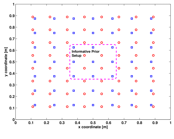
In this section we compare the performance of the considered rules through numerical results. To this end, we consider a 2-D scenario ($\bm{x}_{T}\in\mathbb{R}^{2}$) where a WSN is employed to detect the presence of a target within the region $[0,1]\times[0,1]$, which represents the considered surveillance area. The sensors are arranged according to a regular square grid covering the surveillance area, as shown in Fig. 4.1, where two cases concerning $K=49$ and $K=64$ sensors are illustrated.

Figure 4.1: Regular deployment of WSN in the case of $K=49$ (blue “$\square$” markers) and $K=64$ (red “$\circ$” markers) sensors. The area delimited by magenta dashed line refers to informative prior setup, i.e. $\mathrm{S}_{\bm{x}_{T}}\triangleq[0.35,0.65]\times[0.35,0.65]$.

With reference to the sensing model, for simplicity we assume the same measurement variance for all the sensors, i.e. $\sigma_{w,k}^{2}=\sigma_{w}^{2}$. Also, without loss of generality, we set $\sigma_{w}^{2}=1$. Differently, with reference to the AAF, we will both consider both the cases of ($i$) power-law and ($ii$) exponential AAFs, with parameter values: $\eta=0.2$ (viz. approximate target extent); $\alpha=4$ (power-law AAF decay exponent). Finally, we define the local sensing SNR as $\mathrm{SNR}\triangleq 10\,\log_{10}\frac{\sigma_{s}^{2}}{\sigma_{w}^{2}}$. The local false-alarm rate for every sensor is set to $P_{f,k}=0.05$ (the corresponding decision threshold $\gamma_{k}$ is obtained by inverting relationship in Eq. (2.8)). When not otherwise specified, we assume ideal reporting channels, i.e. $P_{e,k}=0$, $k\in\mathcal{K}$.

With reference to grid-based approaches (cf. Sec. 3.4), those employed for $\bm{x}_{T}$ and $\sigma_{s}^{2}$ are the following:

• Target position $\bm{x}_{T}$: the search (resp. integration) space corresponds to the surveillance area, i.e. $\mathrm{S}_{\bm{x}_{T}}=[0,1]\times[0,1]$. The x-and y-coordinates grid spacings are given by $(1/N_{x})$, where $N_{x}=100$ is chosen here;

• Target average emitted power $\sigma_{s}^{2}$: the search (resp. integration) space is chosen as

  $$S_{\mathrm{\sigma_{s}^{2}}}=\left[(1-\rho_{s})\cdot\sigma_{s,\mathrm{true}}^{2}\>,\>(1+\rho_{s})\cdot\sigma_{s,\mathrm{true}}^{2}\right]\,,$$ (4.1)

  where $\sigma_{s,\mathrm{true}}^{2}$ denotes the emitted power true value and $\rho_{s}=\frac{1}{10}$, which provides a relative $20\%$ uncertainty with respect to $\sigma_{s,\mathrm{true}}^{2}$. The grid spacing is given by $\frac{2\rho_{s}\sigma_{s,\mathrm{true}}^{2}}{N_{\sigma}}$, where $N_{\sigma}=10$ is chosen here;

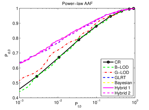
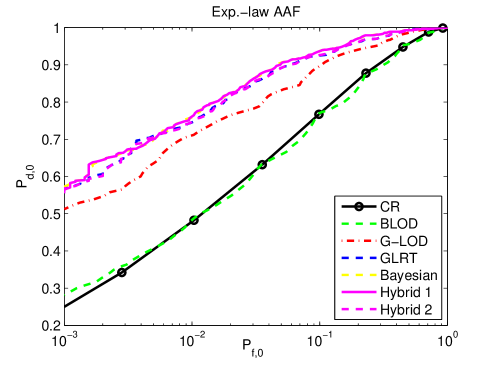
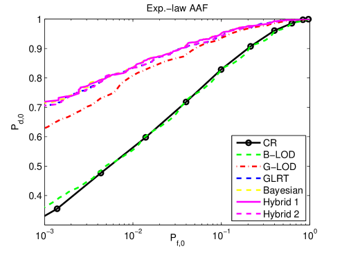
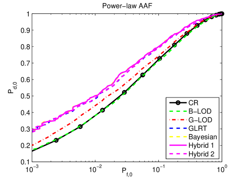
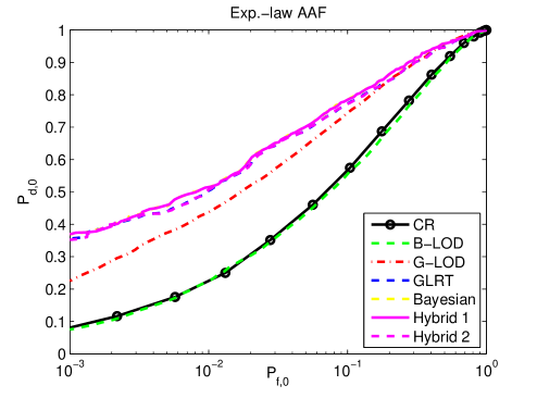
In what follows we compare the considered rules through their corresponding ROCs based on Monte Carlo simulations, obtained with $10^{5}$ runs. The ROC performance reported refer to a scenario where $\bm{x}_{T}$ is uniformly randomly generated at each run within the surveillance area $\mathrm{S}_{\bm{x}_{T}}$.

First, in Fig. 4.2 we report the ROCs for both the cases of power-law AAF (subfigure ($a$)) and exponential AAF (subfigure ($b$)) in a WSN with $K=49$ sensors arranged as in Fig. 4.1 (blue “$\square$” markers). First of all, it is apparent that B-LOD and CR achieve almost the same performance in this scenario. Therefore, the prior information on $\bm{x}_{T}$ is too vague and does not provide itself a relevant gain w.r.t. “blind assumption” of CR, which also arises from different founding rationales (cf. Sec. 2.3). Differently, all the other rules achieve a significant performance improvement over CR. Moreover, purely Bayesian and GLRT approaches, as well as the hybrid ones, roughly achieve the same performance under both power-law and exponential AAFs. Interestingly, G-LOD achieves a worth performance gain w.r.t. CR, especially in the case of an exponential AAF. This is motivated by a faster signal decay (viz. a more “sensitive” spatial signature), which is effectively exploited by the maximization required for G-LOD implementation (see Eq. (3.54)). Also, from inspection of the figures, G-LOD suffers from a slight performance loss when compared to remaining grid-based approaches. However, such loss is balanced by a significant lower complexity required, thus confirming its attractiveness.

(a) Power-law AAF.

(b) Exponential AAF.

Figure 4.2: $P_{d,0}$ vs. $P_{f,0}$ for all the presented rules; WSN with $K=49$ sensors, $\mathrm{SNR}=10\,\mathrm{dB}$, $P_{e,k}=0$ (ideal reporting channels).

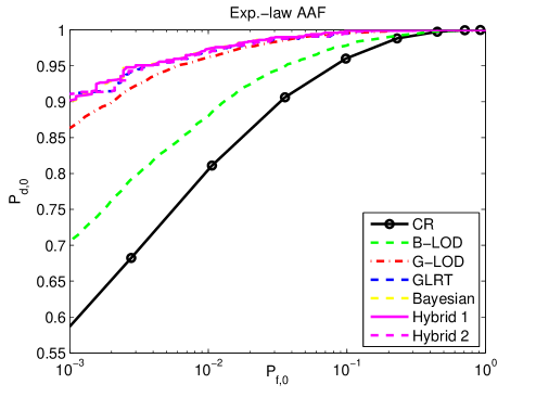
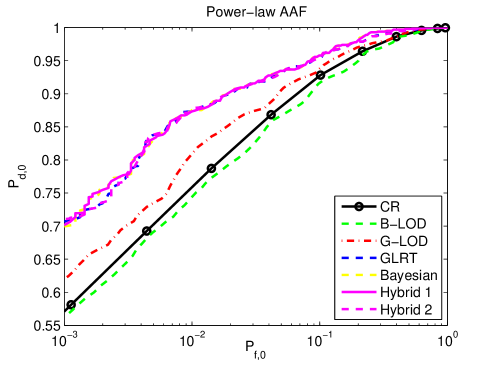
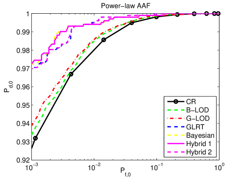
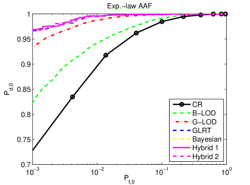
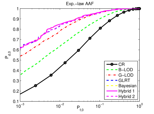
Differently, in Fig. 4.3 we report similar ROCs for the case of a more informative prior availability on $\bm{x}_{T}$. More specifically, we assume that $\bm{x}_{T}\in\mathrm{S}_{\bm{x}_{T}}\triangleq[0.35,0.65]\times[0.35,0.65]$ (see Fig. 4.1), i.e. the target can be located (when present) within a smaller square than the WSN deployment region (see Fig. 4.1). By looking at the figure, similar considerations can be also drawn in this setup, except for the ROC performance achieved by B-LOD. Indeed, in the latter case, the exploitation of the more informative prior pdf $p(\bm{x}_{T})$ available (i.e. a uniform one on a smaller area) overcomes the blind nature behind CR derivation. Therefore, when accurate information on target potential position is available, B-LOD represents an interesting alternative rule, since its complexity grows only linearly with the number of sensors $K$ (cf. Tab. 1).

(a) Power-law AAF.

(b) Exponential AAF.

Figure 4.3: $P_{d,0}$ vs. $P_{f,0}$ for all the presented rules (informative prior setup); WSN with $K=49$ sensors, $\mathrm{SNR}=10\,\mathrm{dB}$, $P_{e,k}=0$ (ideal reporting channels).

Then, in Figs. 4.4 and 4.5 we illustrate performance for the previous two setups (common and informative setups) in the case of $K=64$ sensors (i.e. a more densely deployed WSN), arranged as shown in Fig. 4.1 (red “$\circ$” markers). It is apparent that all rules benefit from an increase of the number of sensors. Nonetheless, analogous trends as the case $K=49$ can be observed.

(a) Power-law AAF.

(b) Exponential AAF.

Figure 4.4: $P_{d,0}$ vs. $P_{f,0}$ for all the presented rules; WSN with $K=64$ sensors, $\mathrm{SNR}=10\,\mathrm{dB}$, $P_{e,k}=0$ (ideal reporting channels).

(a) Power-law AAF.

(b) Exponential AAF.

Figure 4.5: $P_{d,0}$ vs. $P_{f,0}$ for all the presented rules (informative prior setup); WSN with $K=64$ sensors, $\mathrm{SNR}=10\,\mathrm{dB}$, $P_{e,k}=0$ (ideal reporting channels).

Finally, in Figs. 4.6 and 4.7 we show ROCs for the previous setups (assuming $K=64$) in the case of imperfect reporting channels. More specifically, for simplicity we assume the same BEP for all the sensors, i.e. $P_{e,k}=P_{e}$, $k\in\mathcal{K}$, and we set $P_{e}=0.1$. From both figures it is apparent a general degradation of performance due to imperfect reporting channels. Additionally, it can be observed a general decrease of the performance spread for the considered rules. The reason is that a non-zero BEP tends to smooth the spatial signature of the AAF. Additionally, the equal BEP assumption leads to a similar relative confidence of each sensor local decision. Therefore the relative performance loss incurred by CR decreases.

Finally, in Tabs. 2 and 3, we report a comparison of all the presented rules in terms of $P_{d,0}$ (assuming $K=64$ and $\mathrm{SNR=10\,\mathrm{dB}}$) for the relevant scenario of $P_{f,0}=10^{-2}$, in both the previously considered cases of uninformative and informative prior ($p(\bm{x}_{T})$), respectively. As an example, in Tab. 2 when $P_{e,k}=0$ and the assumed AAF follows the exponential law, G-LOD is able to provide a $26\%$ improvement of the detection rate with respect to B-LOD and CR.

(a) Power-law AAF.

(b) Exponential AAF.

Figure 4.6: $P_{d,0}$ vs. $P_{f,0}$ for all the presented rules; WSN with $K=64$ sensors, $\mathrm{SNR}=10\,\mathrm{dB}$, $P_{e,k}=0.1$ (imperfect reporting channels).

(a) Power-law AAF.

(b) Exponential AAF.

Figure 4.7: $P_{d,0}$ vs. $P_{f,0}$ for all the presented rules (informative prior setup); WSN with $K=64$ sensors, $\mathrm{SNR}=10\,\mathrm{dB}$, $P_{e,k}=0.1$ (imperfect reporting channels).

Fusion Rule	Pow-Law,	Exp-Law,	Pow-Law,	Exp-Law,
	$P_{e,k}=0$	$P_{e,k}=0$	$P_{e,k}=0.1$	$P_{e,k}=0.1$
$\Lambda_{\mathrm{G}}$	$0.87$	$0.83$	$0.49$	$0.50$
$\Lambda_{\mathrm{B}}$	$0.87$	$0.83$	$0.5$	$0.51$
$\Lambda_{\mathrm{GB1}}$	$0.87$	$0.83$	$0.5$	$0.51$
$\Lambda_{\mathrm{GB2}}$	$0.87$	$0.83$	$0.49$	$0.50$
$\Lambda_{{\scriptscriptstyle\mathrm{BLOD}}}$	$0.75$	$0.55$	$0.38$	$0.23$
$\Lambda_{{\scriptscriptstyle\mathrm{CR}}}$	$0.77$	$0.55$	$0.38$	$0.23$
$\Lambda_{{\scriptscriptstyle\mathrm{GLOD}}}$	$0.81$	$0.81$	$0.44$	$0.44$

Table 2: Global detection probability ($P_{d,0})$ comparison for the presented rules (global false-alarm rate is set to $P_{f,0}=10^{-2}$). WSN with $K=64$ sensors, $\mathrm{SNR}=10\,\mathrm{dB}$.

Fusion Rule	Pow-Law,	Exp-Law,	Pow-Law,	Exp-Law,
	$P_{e,k}=0$	$P_{e,k}=0$	$P_{e,k}=0.1$	$P_{e,k}=0.1$
$\Lambda_{\mathrm{G}}$	$0.99$	$0.99$	$0.83$	$0.83$
$\Lambda_{\mathrm{B}}$	$0.99$	$0.99$	$0.84$	$0.85$
$\Lambda_{\mathrm{GB1}}$	$0.99$	$0.99$	$0.83$	$0.85$
$\Lambda_{\mathrm{GB2}}$	$0.99$	$0.99$	$0.84$	$0.83$
$\Lambda_{{\scriptscriptstyle\mathrm{BLOD}}}$	$0.98$	$0.94$	$0.78$	$0.64$
$\Lambda_{{\scriptscriptstyle\mathrm{CR}}}$	$0.97$	$0.90$	$0.72$	$0.47$
$\Lambda_{{\scriptscriptstyle\mathrm{GLOD}}}$	$0.98$	$0.98$	$0.78$	$0.78$

Table 3: Global detection probability ($P_{d,0})$ comparison for the presented rules (global false-alarm rate is set to $P_{f,0}=10^{-2}$). WSN with $K=64$ sensors (informative prior setup), $\mathrm{SNR}=10\,\mathrm{dB}$.

5 Conclusions and Future Directions

In this paper we tackled distributed detection of a non-cooperative target. Sensors measure an unknown random signal (embedded in Gaussian noise) with an AAF depending on the distance between the sensor and the target (unknown) positions. Each local decision, based on (local) energy detection, is then sent to a FC for improved detection performance. The focus of this work has concerned the development of practical fusion rules at the FC. To this end, we first focused on the scenario where the emitted power is available at the FC and analyzed fusion rules based on GLRT and Bayesian approaches. Then we moved to the more realistic case of unknown target location ($\bm{x}_{T}$) and power ($\sigma_{s}^{2}$). Such case is typical when detecting non-cooperative targets. The present problem has been formally cast as a one-sided hypothesis testing with nuisance parameters (i.e. $\bm{x}_{T}$) which are present only under $\mathcal{H}_{1}$ (viz. target-present hypothesis). For the resulting hypothesis testing, we analyzed several fusion rules based on: ($i)$ GLRT, ($ii$) Bayesian approach and ($iii$) hybrid combinations of the two. All these rules have been shown to achieve similar performance in all the scenarios being considered. Unfortunately, they all require a grid-based implementation on the Cartesian product of optimization (integration) space of $\bm{x}_{T}$ and $\sigma_{s}^{2}$. Then, with the intent of reducing the computational complexity required by all these approaches, we proposed other two (sub-optimal) fusion rules built upon the LOD framework [22] and based on the following specific rationales:

• B-LOD: $\bm{x}_{T}$ is treated as a random parameter with a prior pdf $p(\bm{x}_{T})$, while $\sigma_{s}^{2}$ is tackled under the LOD framework;

• G-LOD: A generalized version of LOD (based on [23]), arising from maximization (w.r.t. nuisance parameter $\bm{x}_{T}$) of a family of LOD decision statistics obtained by assuming $\bm{x}_{T}$ known;

The aforementioned rules present reduced complexity with respect to the previous rules, all requiring a grid-based search or integration with respect to both $\bm{x}_{T}$ and $\sigma_{s}^{2}$. More specifically, B-LOD retains a linear complexity in the number of sensors (as the simple CR), while G-LOD is based on a (reduced) grid search which only requires optimization w.r.t. $\bm{x}_{T}$. Additionally, G-LOD has been shown to outperform CR in all the considered cases and to incur in a moderate performance loss with respect to other rules requiring grid implementation on both parameters. Differently, B-LOD has been shown to provide a significant gain over CR only when the prior pdf of $\bm{x}_{T}$ is informative enough.

All the considered rules have been extended to the case of imperfect reporting channels, modeled as BSCs with corresponding BEPs $P_{e,k}$ assumed known at the FC. It has been demonstrated that only a slight modification of their expressions is required in order to account for this additional uncertainty, whereas it has been observed that non-zero BEPs tend to smooth the spatial signature determined by the AAF and thus to reduce the gain obtained by all the rules exploiting spatial information of the target w.r.t. CR.

Future works will include the design and analysis of fusion rules based on soft-decisions (i.e. multi-bit quantization) from the sensors, as well as the problem of detecting time-evolving (diffusive) sources with possibly moving sensors. Both the cases of cooperative and uncooperative targets are of interest. Furthermore, the case of uncertain sensors positions will be tackled in comparison to the well-known concept of scan statistics [18]. Finally, robust design of fusion rules accounting for uncertainties at the reporting channels (i.e. unknown BEPs) will be also considered.

Appendix

Derivation of Bayesian LOD

In this Appendix, we derive the explicit expression of the LOD [22] based on a prior distribution assumption for the target position $\bm{x}_{T}$, that is based on Eq. (3.22). To this end, starting from the implicit form in (3.45), we first concentrate on obtaining the closed form of $\frac{\partial\ln\left[P(\bm{d}|\mathcal{H}_{1};\theta)\right]}{\partial\theta}$. The latter term is obtained recalling that:

$$\ln\left[P(\bm{d}|\mathcal{H}_{1};\theta)\right]=\ln\left[\int\prod_{k=1}^{K}P_{d,k}(\bm{x}_{T},\theta)^{d_{k}}\left[1-P_{d,k}(\bm{x}_{T},\theta)\right]^{(1-d_{k})}\,p(\bm{x}_{T})\,d\bm{x}_{T}\right]\,.$$ (5.1)

The derivative of the log-pdf can be thus obtained in closed form as:

$$\frac{\partial\ln\left[P(\bm{d}|\mathcal{H}_{1};\theta)\right]}{\partial\theta}=\frac{\int\frac{\partial P(\bm{d}|\mathcal{H}_{1};\bm{x}_{T},\theta)}{\partial\theta}\,p(\bm{x}_{T})\,d\bm{x}_{T}}{\int\prod_{k=1}^{K}P_{d,k}(\bm{x}_{T},\theta)^{d_{k}}\left[1-P_{d,k}(\bm{x}_{T},\theta)\right]^{(1-d_{k})}\,p(\bm{x}_{T})\,d\bm{x}_{T}}\,,$$ (5.2)

where we have interchanged the order of derivative and integration at the numerator. Also, the derivative within the integral in (5.2) at the numerator can be evaluated in explicit form as:

$$\frac{\partial P(\bm{d}|\mathcal{H}_{1};\bm{x}_{T},\theta)}{\partial\theta}= \left(\prod_{k=1}^{K}P_{d,k}(\bm{x}_{T},\theta)^{d_{k}}\left[1-P_{d,k}(\bm{x}_{T},\theta)\right]^{(1-d_{k})}\right)\,$$

$$\times\sum_{k=1}^{K}\frac{d_{k}-P_{d,k}(\bm{x}_{T},\theta)}{P_{d,k}(\bm{x}_{T},\theta)\left[1-P_{d,k}(\bm{x}_{T},\theta)\right]}\frac{\partial P_{d,k}(\bm{x}_{T},\theta)}{\partial\theta}\,.$$ (5.3)

For the considered model in Eq. (2.8), the derivative of the $P_{d,k}$ w.r.t. $\theta$ is given explicitly as:

$$\frac{\partial P_{d,k}(\bm{x}_{T},\theta)}{\partial\theta} =2\,\frac{\partial}{\partial\theta}\mathcal{Q}\left(\sqrt{\frac{\gamma_{k}}{\sigma_{w,k}^{2}+\theta\,g^{2}(\bm{x}_{T},\bm{x}_{k})}}\right)$$ (5.4)

$$=p_{w}\left(\sqrt{\frac{\gamma_{k}}{\sigma_{w,k}^{2}+\theta\,g^{2}(\bm{x}_{T},\bm{x}_{k})}}\right)\frac{\sqrt{\gamma_{k}}\,g^{2}(\bm{x}_{T},\bm{x}_{k})}{\left[\sigma_{w,k}^{2}+\theta\,g^{2}(\bm{x}_{T},\bm{x}_{k})\right]^{3/2}}\,.$$ (5.5)

Evaluating the derivative of the log-pdf in (5.2) at $\theta=\theta_{0}$ (which corresponds to null hypothesis $\mathcal{H}_{0}$, see Eq. (3.8)), leads to

$$\left.\frac{\partial\ln\left[P(\bm{d}|\mathcal{H}_{1};\theta)\right]}{\partial\theta}\right|_{\theta=\theta_{0}}=\frac{\int\left.\frac{\partial P(\bm{d};\mathcal{H}_{1},\bm{x}_{T},\theta)}{\partial\theta}\right|_{\theta=0}\,p(\bm{x}_{T})\,d\bm{x}_{T}}{\prod_{k=1}^{K}(P_{f,k})^{d_{k}}(1-P_{f,k})^{(1-d_{k})}}\,,$$ (5.6)

where, exploiting (5.3), we obtain:

$$\left.\frac{\partial P(\bm{d}|\mathcal{H}_{1};\bm{x}_{T},\theta)}{\partial\theta}\right|_{\theta=\theta_{0}}=\left(\prod_{k=1}^{K}(P_{f,k})^{d_{k}}\left[1-P_{f,k}\right]^{(1-d_{k})}\right)\sum_{k=1}^{K}\frac{d_{k}-P_{f,k}}{P_{f,k}\left(1-P_{f,k}\right)}\left.\frac{\partial P_{d,k}(\bm{x}_{T},\theta)}{\partial\theta}\right|_{\theta=\theta_{0}}\,,$$ (5.7)

and in turn (cf. Eq. (5.5))

$$\left.\frac{\partial P_{d,k}(\bm{x}_{T},\theta)}{\partial\theta}\right|_{\theta=\theta_{0}}=p_{w}\left(\sqrt{\frac{\gamma_{k}}{\sigma_{w,k}^{2}}}\right)\frac{\sqrt{\gamma_{k}}\,g^{2}(\bm{x}_{T},\bm{x}_{k})}{\left(\sigma_{w,k}^{2}\right)^{3/2}}\,.$$ (5.8)

Then, exploiting the appropriate substitutions, we obtain:

$$\left.\frac{\partial\ln\left[P(\bm{d}|\mathcal{H}_{1};\theta)\right]}{\partial\theta}\right|_{\theta=\theta_{0}}=\sum_{k=1}^{K}\frac{d_{k}-P_{f,k}}{P_{f,k}\left(1-P_{f,k}\right)}\,p_{w}\left(\sqrt{\frac{\gamma_{k}}{\sigma_{w,k}^{2}}}\right)\frac{\sqrt{\gamma_{k}}}{\left(\sigma_{w,k}^{2}\right)^{3/2}}\left(\int g^{2}(\bm{x}_{T},\bm{x}_{k})\,p(\bm{x}_{T})\,d\bm{x}_{T}\right)\,.$$ (5.9)

Now we show how to obtain the explicit form of the FI evaluated at $\theta_{0}$. First, we start from the common definition:

$$I(\theta_{0})=\mathbb{E}_{P(\bm{d}|\mathcal{H}_{0})}\left\{\left(\left.\frac{\partial\ln\left[P(\bm{d}|\,\mathcal{H}_{1};\theta)\right]}{\partial\theta}\right|_{\theta=\theta_{0}}\right)^{2}\right\}\,.$$ (5.10)

Since the elements $d_{k}$, $k=1,\ldots K$, are uncorrelated it holds that:

$$I(\theta_{0})=\sum_{k=1}^{K}\frac{\mathbb{E}\left\{\left(d_{k}-P_{f,k}\right)^{2}\right\}}{P_{f,k}^{2}\left(1-P_{f,k}\right)^{2}}\,p_{w}^{2}\left(\sqrt{\frac{\gamma_{k}}{\sigma_{w,k}^{2}}}\right)\frac{\gamma_{k}}{\left(\sigma_{w,k}^{2}\right)^{3}}\left(\int g^{2}(\bm{x}_{T},\bm{x}_{k})\,p(\bm{x}_{T})\,d\bm{x}_{T}\right)^{2}\,.$$ (5.11)

Evaluating the expectation inside the above equation, provides the explicit form of $I(\theta_{0})$:

$$I(\theta_{0})=\sum_{k=1}^{K}\frac{1}{P_{f,k}\left(1-P_{f,k}\right)}\,p_{w}^{2}\left(\sqrt{\frac{\gamma_{k}}{\sigma_{w,k}^{2}}}\right)\frac{\gamma_{k}}{\left(\sigma_{w,k}^{2}\right)^{3}}\left(\int g^{2}(\bm{x}_{T},\bm{x}_{k})\,p(\bm{x}_{T})\,d\bm{x}_{T}\right)^{2}\,.$$ (5.12)

Substitution of closed forms of Eqs. (5.9) and (5.12) into the implicit form in (3.23), provides the explicit expression reported in Eq. (3.25).

Derivation of Generalized LOD

In this Appendix, we derive the explicit expression of the G-LOD proposed by Davies. To this end, we concentrate on finding the explicit form of LOD fusion rule [22] assuming $\bm{x}_{T}$ known. Once obtained, the explicit expression will clearly depend on $\bm{x}_{T}$. Such expression will be then plugged in the maximization of Eq. (3.29) to obtain the final statistic. First, we observe that:

$$\frac{\partial\ln P(\bm{d}|\mathcal{H}_{1};\bm{x}_{T},\theta)}{\partial\theta}=\sum_{k=1}^{K}\frac{d_{k}-P_{d,k}(\bm{x}_{T},\theta)}{P_{d,k}(\bm{x}_{T},\theta)\left[1-P_{d,k}(\bm{x}_{T},\theta)\right]}\frac{\partial P_{d,k}(\bm{x}_{T},\theta)}{\partial\theta}\,,$$ (5.13)

where $\frac{\partial P_{d,k}(\bm{x}_{T},\theta)}{\partial\theta}$ is defined as in Eq. (5.5). Setting $\theta=\theta_{0}$, the above term reduces to:

$$\left.\frac{\partial\ln P(\bm{d}|\mathcal{H}_{1};\bm{x}_{T},\theta)}{\partial\theta}\right|_{\theta=\theta_{0}}=\sum_{k=1}^{K}\frac{d_{k}-P_{f,k}}{P_{f,k}(1-P_{f,k})}\,p_{w}\left(\sqrt{\frac{\gamma_{k}}{\sigma_{w,k}^{2}}}\right)\frac{\sqrt{\gamma_{k}}\,g^{2}(\bm{x}_{T},\bm{x}_{k})}{\left(\sigma_{w,k}^{2}\right)^{3/2}}\,,$$ (5.14)

where we exploited the definition in Eq. (5.5). Similarly, exploiting (conditional) independence of the decisions $d_{k}$, $k=1,\ldots K$, we obtain:

$$I(\bm{x}_{T},\theta)=\sum_{k=1}^{K}I_{k}(\bm{x}_{T},\theta)\,,$$ (5.15)

where we have denoted with $I_{k}(\bm{x}_{T},\theta)$ the contribution of $k$th to the FI, that is:

$$I_{k}(\bm{x}_{T},\theta) =\mathbb{E}\left\{\left(\frac{\partial\ln\left[P(d_{k}|\mathcal{H}_{1};\bm{x}_{T},\theta)\right]}{\partial\theta}\right)^{2}\right\}$$ (5.16)

$$=\frac{\mathbb{E}\left\{\left[d_{k}-P_{d,k}(\bm{x}_{T},\theta)\right]^{2}\right\}}{P_{d,k}(\bm{x}_{T},\theta)^{2}\left[1-P_{d,k}(\bm{x}_{T},\theta)\right]^{2}}\left(\frac{\partial P_{d,k}(\bm{x}_{T},\theta)}{\partial\theta}\right)^{2}$$ (5.17)

$$=\frac{1}{P_{d,k}(\bm{x}_{T},\theta)\left[1-P_{d,k}(\bm{x}_{T},\theta)\right]}\left(\frac{\partial P_{d,k}(\bm{x}_{T},\theta)}{\partial\theta}\right)^{2}$$ (5.18)

where, in obtaining the last line we have explicitly evaluated the expectation in Eq. (5.17). Then, substitution $\theta\rightarrow\theta_{0}$ in $I(\bm{x}_{T},\theta)$ provides:

$$I(\bm{x}_{T},\theta_{0})\;= \sum_{k=1}^{K}I_{k}(\bm{x}_{T},\theta_{0})$$ (5.19)

$$= \sum_{k=1}^{K}\frac{1}{P_{f,k}\left[1-P_{f,k}\right]}p_{w}^{2}\left(\sqrt{\frac{\gamma_{k}}{\sigma_{w,k}^{2}}}\right)\frac{\gamma_{k}\,g^{4}(\bm{x}_{T},\bm{x}_{k})}{\left(\sigma_{w,k}^{2}\right)^{3}}\,.$$ (5.20)

Exploiting Eqs. (5.20) and (5.14) into (3.29), provides the final expression in (3.31).

References

- [1] D. Ding, Z. Wang, H. Dong, H. Shu, Distributed H-inf state estimation with stochastic parameters and nonlinearities through sensor networks: The finite-horizon case, Automatica 48 (8) (2012) 1575–1585.
- [2] D. Ding, Z. Wang, B. Shen, H. Dong, Event-triggered distributed H-Inf state estimation with packet dropouts through sensor networks, IET Control Theory & Applications 9 (13) (2015) 1948–1955.
- [3] C.-Y. Chong, S. P. Kumar, Sensor networks: evolution, opportunities, and challenges, Proceedings of the IEEE 91 (8) (2003) 1247–1256.
- [4] P. K. Varshney, Distributed Detection and Data Fusion, 1st Edition, Springer-Verlag New York, Inc., 1996.
- [5] D. Ciuonzo, G. Papa, G. Romano, P. Salvo Rossi, P. Willett, One-bit decentralized detection with a Rao test for multisensor fusion, IEEE Signal Processing Letters 20 (9) (2013) 861–864.
- [6] J. Fang, Y. Liu, H. Li, S. Li, One-bit quantizer design for multisensor GLRT fusion, IEEE Signal Processing Letters 20 (3) (2013) 257–260.
- [7] D. Ciuonzo, P. Salvo Rossi, Decision fusion with unknown sensor detection probability, IEEE Signal Processing Letters 21 (2) (2014) 208–212.
- [8] D. Ciuonzo, A. De Maio, P. Salvo Rossi, A systematic framework for composite hypothesis testing of independent Bernoulli trials, IEEE Signal Processing Letters 22 (9) (2015) 1249–1253.
- [9] P. Salvo Rossi, D. Ciuonzo, T. Ekman, H. Dong, Energy detection for MIMO decision fusion in underwater sensor networks, IEEE Sensors Journal 15 (3) (2015) 1630–1640.
- [10] P. Salvo Rossi, D. Ciuonzo, K. Kansanen, T. Ekman, On energy detection for MIMO decision fusion in wireless sensor networks over NLOS fading., IEEE Communications Letters 19 (2) (2015) 303–306.
- [11] Z. Chair, P. K. Varshney, Optimal data fusion in multiple sensor detection systems, IEEE Transactions on Aerospace and Electronic Systems AES-22 (1) (1986) 98–101.
- [12] S. M. Kay, Fundamentals of Statistical Signal Processing, Volume 2: Detection Theory, Prentice Hall PTR, 1998.
- [13] R. Niu, P. K. Varshney, Q. Cheng, Distributed detection in a large wireless sensor network, Information Fusion 7 (4) (2006) 380–394, special Issue on the 7th International Conference on Information Fusion-Part I.
- [14] R. Niu, P. K. Varshney, Performance analysis of distributed detection in a random sensor field, IEEE Transactions on Signal Processing 56 (1) (2008) 339–349.
- [15] N. Katenka, E. Levina, G. Michailidis, Local vote decision fusion for target detection in wireless sensor networks, IEEE Transactions on Signal Processing 56 (1) (2008) 329–338.
- [16] M. S. Ridout, An improved threshold approximation for local vote decision fusion, IEEE Transactions on Signal Processing 61 (5) (2013) 1104–1106.
- [17] R. Niu, P. K. Varshney, Joint detection and localization in sensor networks based on local decisions, in: 40th Asilomar Conference on Signals, Systems and Computers, 2006, pp. 525–529.
- [18] M. Guerriero, P. Willett, J. Glaz, Distributed target detection in sensor networks using scan statistics, IEEE Transactions on Signal Processing 57 (7) (2009) 2629–2639.
- [19] M. Guerriero, L. Svensson, P. K. Willett, Bayesian data fusion for distributed target detection in sensor networks, IEEE Transactions on Signal Processing 58 (6) (2010) 3417–3421.
- [20] A. Shoari, A. Seyedi, Detection of a non-cooperative transmitter in Rayleigh fading with binary observations, in: IEEE Military Communications Conference (MILCOM), 2012, pp. 1–5.
- [21] Y. Sung, L. Tong, A. Swami, Asymptotic locally optimal detector for large-scale sensor networks under the Poisson regime, IEEE Transactions on Signal Processing 53 (6) (2005) 2005–2017.
- [22] S. A. Kassam, J. B. Thomas, Signal detection in non-Gaussian noise, Springer-Verlag New York, 1988.
- [23] R. D. Davies, Hypothesis testing when a nuisance parameter is present only under the alternative, Biometrika 74 (1) (1987) 33–43.
- [24] E. L. Lehmann, J. P. Romano, Testing statistical hypotheses, Springer Science & Business Media, 2006.
- [25] A. S. Gupta, L. Vermeire, Locally optimal tests for multiparameter hypotheses, J. Am. Stat. Assoc. 81 (395) (1986) 819–825.
- [26] J. O. Berger, B. Liseo, R. L. Wolpert, Integrated likelihood methods for eliminating nuisance parameters, Statistical Science 14 (1) (1999) 1–28.
- [27] D. Ciuonzo, G. Romano, P. Salvo Rossi, Channel-aware decision fusion in distributed MIMO wireless sensor networks: Decode-and-fuse vs. decode-then-fuse, IEEE Transactions on Wireless Communications 11 (8) (2012) 2976–2985.
- [28] D. Ciuonzo, P. Salvo Rossi, S. Dey, Massive MIMO channel-aware decision fusion, IEEE Transactions on Signal Processing 63 (3) (2015) 604–619.
- [29] J. Proakis, Digital Communications, 4th Edition, McGraw-Hill Science/Engineering/Math, 2000.
- [30] S. Chaudhari, J. Lundén, V. Koivunen, H. V. Poor, Cooperative sensing with imperfect reporting channels: Hard decisions or soft decisions?, IEEE Transactions on Signal Processing 60 (1) (2012) 18–28.