Comparative study of space filling curves for cache oblivious TU Decomposition

Abstract

We examine several matrix layouts based on space-filling curves that allow for a cache-oblivious adaptation of parallel TU decomposition for rectangular matrices over finite fields. The TU algorithm of [11] requires index conversion routines for which the cost to encode and decode the chosen curve is significant. Using a detailed analysis of the number of bit operations required for the encoding and decoding procedures, and filtering the cost of lookup tables that represent the recursive decomposition of the Hilbert curve, we show that the Morton-hybrid order incurs the least cost for index conversion routines that are required throughout the matrix decomposition as compared to the Hilbert, Peano, or Morton orders. The motivation lies in that cache efficient parallel adaptations for which the natural sequential evaluation order demonstrates lower cache miss rate result in overall faster performance on parallel machines with private or shared caches, on GPU’s, or even cloud computing platforms. We report on preliminary experiments that demonstrate how the TURBO algorithm in Morton-hybrid layout attains orders of magnitude improvement in performance as the input matrices increase in size. For example, when $N=2^{13}$, the row major TURBO algorithm concludes within about 38.6 hours, whilst the Morton-hybrid algorithm with truncation size equal to $64$ concludes within 10.6 hours.

1 Introduction

Exact triangulisation of matrices is crucial for a large range of problems in Computer Algebra and Algorithmic Number Theory, where a basis of the solution set of the associated linear system is required. A known algorithm in the field which resulted in several prominent adaptations is the TURBO algorithm of Dumas et al. [11] for exact LU decomposition. This algorithm recurses on rectangular and potentially singular matrices, which makes it possible to take advantage of cache effects. It improves on other expensive methods for handling singular matrices, which otherwise have to dynamically adjust the submatrices so that they become invertible. Particularly, TURBO significantly reduces the volume of communication on distributed architectures, and retains optimal work and linear span. TURBO can also compute the rank in an exact manner. As benchmarked against some of the most efficient exact elimination algorithms in the literature, TURBO incurs low synchronisation costs and reduces the communication cost featured by [13, 14] by a factor of one third when used with only one level of recursion on 4 processors. In TURBO, local TU factorisations are performed until the sub-matrices reach a given threshold, and so one can take advantage of cache effects. A cache friendly adaptation of the serial version of TURBO bears impact on all possible forms of parallel or distributed deployment of the algorithm. For one, nested parallel algorithms with low depth and for which the natural sequential execution has low cache complexity will also attain good cache complexity on parallel machines with private or shared caches [6]. Locality of reference on distributed systems is also being advocated by the Databricks group initiated by founders of Apache Spark. In their own terms, when profiling Spark user applications on distributed clusters, a large fraction of the CPU time was spent waiting for data to be fetched from main memory. Locality of reference is also of concern on GPUs. Although one does not have full control over optimising locality of reference on such machines, and despite that GPUs rely on thread-level parallelism to hide long latencies associated with memory access, the memory hierarchy remains critical for many applications. Finally, applications that are cache aware are also deemed to be more energy aware, as remarked by the Green computing community.

This preamble motivates our work on trying to improve the cache performance of the serial version of TURBO. It is well established that traditional row-major or column-major layouts of matrices in compilers lead to extremely poor temporal and spatial locality of matrix algorithms. Instead, several matrix layouts based on space filling-curves have yielded cache-oblivious adaptations of matrix algorithms such as matrix-matrix multiplication [5, 9] and matrix factorisation [4, 12, 21]. Those alternative layouts are recursive in nature and produce highly cache-efficient, cache-oblivious adaptations that scale with the size of the underlying matrices. The cache-oblivious model does not require knowledge of, and hence tuning the algorithm according to, the cache parameters. Cache-oblivious programs allow for resource usage not to be programmed explicitly, and for algorithms to be portable across varying architectures, as well as all levels of the memory hierarchy within one specific architecture.

Our contributions can be summarised as follows:

1. We investigate prospects for a cache oblivious adaptation of the TURBO algorithm by mapping four different matrix layouts against each other: the Hilbert order [10, 15], the Peano order [4, 5], the Morton order [16, 20], and the Morton-hybrid order [2]. Whilst matrices on which we want to perform matrix-matrix multiplication or LU decomposition without pivoting can be serialized no matter what layout is used, the recursive TU decomposition considered in this work consistently requires permutation steps that require one to traverse the matrix in a row-wise or column-wise manner, thus eliciting index conversion from the Cartesian scheme to the recursive scheme and vice versa. In addition to the specific contributions summarised below, this survey component of our work

2. Our analysis of the four schemes addresses the cost of bit operations and accessing table lookups when applicable. Our findings show the following:

   1. The overhead for using the Peano layout will be compelling as index conversion invokes operations modulo 3.

   2. Whilst the Hilbert layout has been promising for improving memory performance of matrix algorithms in general, and despite that the operations for encoding and decoding in this layout can be performed using bit shifts and bit masks, we will still require $m$ iterations for a $2^{m}\times 2^{m}$ matrix for each single invocation of encoding or decoding.

   3. In contrast, we find that the conversions for the Morton and the Morton-hybrid layouts incur a constant number of operations assuming the matrix is of dimensions at most $2^{\alpha}\times 2^{\alpha}$, where $\alpha$ is the machine word-size. For the typical value $\alpha=64$, such matrix sizes are sufficiently large for many applications.

   4. Furthermore, despite that the Morton order can be encoded and decoded faster than the Morton-hybrid order, the factor of improvement is constant: ten less operations. In return, the Morton-hybrid layout allows the recursion to stop when the blocks being divided are of some prescribed size equal to $T\times T$ , thus decreasing the recursion overhead. These $T\times T$ blocks are stored in a row-major order, which allows for benefiting from compiler optimizations that have already been designed for this layout. The row-major ordering of the block at the base case also makes accessing the entries within the blocks at the base case of the inversion, multiplication, and decomposition steps of the algorithm faster and easier because no index conversion is required.

3. Unless otherwise stated and explicitly cited, the various encoding and decoding algorithms we present under these various layouts and the propositions/proofs associated with them, are novel.

4. The present manuscript is an indispensable precursor for our work in [1], where we introduce the concepts of alignment of sub-matrices with respect to the cache lines and their containment within proper blocks under the Morton-hybrid layout, and describe the problems associated with the recursive subdivisions of TURBO under this scheme. Although the full details of the resulting algorithm are beyond the scope of this paper, we report on experiments that demonstrate how the TURBO algorithm in Morton-hybrid layout attains orders of magnitude improvement in performance as the input matrices increase in size. For example, when $N=2^{13}$, the row major TURBO algorithm concludes within about 38.6 hours, whilst the Morton-hybrid algorithm with truncation size equal to $64$ concludes within 10.6 hours.

2 The TU Algorithm: A Summary

Consider a $2m\times 2n$ matrix $A$ with rank $r$ over a field $\mathbb{F}$, where $A$ may be singular. The TURBO algorithm triangulates the matrix $A$ in a succession of recursive steps, relaxing the condition for generating a strictly lower triangular matrix. All the recursive steps are independent and thus TURBO is inherently parallel. It further outputs two matrices $T$ and $U$, such that $A=T\cdot U$, where $U$ is a $2m\times 2n$ upper triangular matrix, and $T$ is $2m\times 2m$, with some “$T$” patterns. In all of the following, let $A^{(i,j)}_{{}_{(a,b)}}$ denote the sub-matrix of $A$ of dimensions $a\times b$ and starting at the entry of Cartesian index $(i,j)$. Whenever the superscript $(i,j)$ is omitted, a default value $(0,0)$ is assumed. First, begin by decomposing the matrix $A$ of size $2m\times 2n$ as follows:

$$A_{{}_{(2m,2n)}}=\left(\begin{array}[]{cc}NW_{{}_{(m,n)}}&NE_{{}_{(m,n)}}\\ SW_{{}_{(m,n)}}&SE_{{}_{(m,n)}}\end{array}\right)$$ (1)

The TURBO alogrithm now performs the following:

1. Recursive TU decomposition in each of SE, then SW, NE, and finally, NW

2. Virtual row and column permutations needed to re-order the blocks to yield a final, upper triangular matrix

For brevity, we only elaborate on the first step in the TURBO algorithm. It gives a flavour of the various matrix opertions we will be addressing throughout the paper. The rest of the steps can be found in [11].

2.1 Step 1: Recursive TU in $NW$

This step performs a recursive call to the TU decomposition algorithm in the $NW$ quadrant of $A$ to get $U_{1}$ upper triangular, $G_{1}$, and $L_{1}$, lower triangular, such that

$$L_{1}\cdot NW=\left(\begin{array}[]{cc}U_{1}&G_{1}\\ 0&0\end{array}\right).$$

Here, $U_{1}$ is $r\times r$ for some $r\geq 0$, $G_{1}$, and $L_{1}$ is $m\times m$. $L_{1}$ is then used to update $NE$ by:

$$B_{1_{(m,n)}}=L_{1}\cdot NE.$$

One now aims to zero out the sub-matrix of SW that lies under $U_{1}$. This is done by calculating

$$N_{1_{(m,r)}}=-SW_{{}_{(m,r)}}\cdot U_{1}^{-1}$$

and then setting

$$\left(\begin{array}[]{cc}0_{{}_{(m,r)}}&I_{1_{(m,n-r)}}\end{array}\right)=SW+N_{1_{(m,r)}}\cdot\left(\begin{array}[]{cc}U_{1_{(r,r)}}&G_{1_{(r,n-r)}}.\end{array}\right)$$

The submatrix $SE$ has to be updated accordingly:

$$E_{1}=SE+N_{1}\cdot B_{1}.$$

At the end of this step, matrix $A$ has been updated as follows:

$$A_{1}=\left(\begin{array}[]{ccc}U_{1_{(r,r)}}&G_{1_{(r,n-r)}}&B_{1_{(r,n)}}\\ 0_{{}_{(m-r,r)}}&0_{{}_{(m-r,n-r)}}&B_{1_{(m-r,n)}}\\ 0_{{}_{(m,r)}}&I_{1_{(m,n-r)}}&E_{1_{(m,n)}}\\ \end{array}\right).$$

The resulting matrix can be seen in Fig. 1(a) taken from [11].

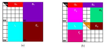
Figure 1: Matrix after Step 1 (a) and Step 2 (b)

3 Comparison of Index Conversion Overhead

The amount of computation required for index conversion from each of the Hilbert, Peano, Morton, and Morton-hybrid layouts to the Cartesian order is used to rate each of these layouts as they apply to TURBO. The row and column permutations required at every level of the recursion make row and column traversals of the matrix crucial. Intensive conversion tasks are required for row and column traversals of the matrices. This makes the overhead of index conversion essential in the comparison of the different layouts available. Let $\Theta$ denote a subscript associated with one of the four layouts named above. Given a Cartesian index $(i,j)$, encoding it in the order $\Theta$ corresponds to calculating its index $z_{\Theta}$ in the resulting matrix layout under $\Theta$.

Given an index $z_{\Theta}$ of a matrix entry under order $\Theta$, decoding $z_{\Theta}$ corresponds to calculating the Cartesian index $(i,j)$.

3.1 Conversion Terms

The following is a list of terminologies used in the remainder of this manuscript.

1. $\&$ : the bitwise AND operator

2. $|$ : the bitwise OR operator

3. $<<$ : the bitwise left shift operator, where $i<<k$ is equivalent to multiplying $i$ by $2^{k}$.

4. $>>$ : the bitwise right shift operator, where $i>>k$ is equivalent to dividing $i$ by $2^{k}$.

5. Masks: These are bit values represented in hexadecimal format. The masks used hereafter are:

   • $0$x$00FF00FF=(00000000111111110000000011111111)_{2}$

   • $0$x$0F0F0F0F=(00001111000011110000111100001111)_{2}$

   • $0$x$33333333=(00110011001100110011001100110011)_{2}$

   • $0$x$55555555=(01010101010101010101010101010101)_{2}$

   • $0$x$0000FFFF=(00000000000000001111111111111111)_{2}$

   • $0$x$AAAAAAAA=(10101010101010101010101010101010)_{2}$

6. The act of masking a value $v$: applying an AND operation on $v$ and a mask to extract part of $v$.

7. The row index of an entry $e$ in a given matrix is its row offset within the matrix. It is given by $i$ from the Cartesian index $(i,j)$ of $e$. The column index of the entry is its column offset, given by $j$.

8. Consider a matrix $M$ decomposed into sub-blocks of size $2^{k}\times 2^{k}$. For any given sub-block, its row index is its row offset within $M$ and its column index is its column offset within $M$.

9. The index of an entry in a given matrix laid out in order $\Theta$ is its offset within the linear array representing the matrix in the layout $\Theta$. This was denoted earlier by $z_{\Theta}$

10. The index of a sub-block of size $2^{k}\times 2^{k}$ in a given matrix laid out in order $\Theta$ is the offset of this sub-block within the linear array of objects representing the matrix in the layout $\Theta$, where each object is a $2^{k}\times 2^{k}$ sub-block.

11. We refer to the index of an entry (or block) in the $\Theta$ order as the $\Theta$ index of this entry (or block). For example, when considering a matrix $M$ laid out in the row-major order, $\Theta$ refers to the row-major order and the row-major index of an entry (or block) of $M$ is the index of this entry (or block) in the row-major layout of $M$.

3.2 Encoding/Decoding in the Row-Major Order

The row-major (column-major) order is the default ordering used by compilers for two dimensional arrays. Computer memory is linear and consists of a list of consecutive addresses in memory. Compilers therefore store a two dimensional array by laying it out row by row. When the programmer uses the notation $A[i][j]$ to access the element in position $(i,j)$ of the matrix $A$, the compiler performs the index conversion behind the scenes. In the rest of this section, we consider the example matrix shown in Fig. 2 with $n=8$ i.e. $m=3$, and take $\Theta$ to denote the row-major order.

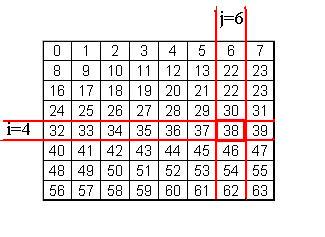
Figure 2: Row Major Ordered Matrix

3.2.1 Encoding in the Row-Major Order

Consider the Cartesian index $(i,j)$ in a matrix laid out in a row-major fashion. To find $z_{\Theta}(i,j,n)$, denoted by $z_{\Theta}$ for simplicity, use the equation

$$z_{\Theta}=i\times n+j.$$ (2)

For the example shown in Fig. 2, to encode $i=4$ and $j=6$, using Eq. (2) results in $z_{\Theta}=4\times 8+6=32+6=38$. Because the element of Cartesian index $(i,j)$ lies within a $2^{m}\times 2^{m}$ matrix, then $i,j\in\{0,1,2,...,2^{m}\}$, and so, to represent any of these values in the binary system, at most $m$ bits are needed. Write

$$i=(i_{m-1}....i_{3}i_{2}i_{1}i_{0})_{2}$$

and

$$j=(j_{m-1}....j_{3}j_{2}j_{1}j_{0})_{2}.$$

The integer operations to find $z_{\Theta}$ given by Eq. (2) are equivalent to the following bit operations:

$$z_{\Theta}=(i<<m)|j$$

for $n=2^{m}$. This can be seen as concatenating the bits of $j$ to the bits of $i$ to get:

$$z_{\Theta}=(i_{m-1}...i_{3}i_{2}i_{1}i_{0}j_{m-1}...j_{3}j_{2}j_{1}j_{0})_{2}.$$

Hence, the encoding can be done using bit shifting and bit masking operations on the binary representations of $i$ and $j$, as shown in Alg. 1. For $i=4$ and $j=6$ represented as $i=(100)_{2}$ and $j=(110)_{2}$, $i<<3=(100000)_{2}$ and $z_{\Theta}=(100000)_{2}|(110)_{2}=(100110)_{2}=38$.

1

2$z_{\Theta}$ = ( $i$ $<<$ $m$ ) $|$ $j$

Algorithm 1 Encoding for the Row-Major Order Using Bit Operations

3.2.2 Decoding in the Row-Major Order

$$i=z_{\Theta}\div n$$ (3)

$$j=z_{\Theta}\%n$$ (4)

Equations Eq. (3) and Eq. (4) present the operations used for decoding an index in the row-major order using integer operations. These equations follow from Eq. (2) by which we obtain $z_{\Theta}$ as:

$$z_{\Theta}=i\times n+j$$

In Eq. (3) and Eq. (4), we extract the $i$ and $j$ value of the index $(i,j)$ respectively. Using these equations to decode the index 38 from Fig. 2, compute $i=38\div 8=4$ and $j=38\%8=6$. Alg. 2 describes the corresponding bit operations. Recall that $n=2^{m}$, so the extraction of $i$ given by Eq. (3) can be done using the bit operations:

$$i=z_{\Theta}>>m$$

and the extraction of $j$ given by Eq. (4) can be done using:

$$j=z_{\Theta}\&(2^{m}-1).$$

To decode $z_{\Theta}=38$, one operates on the bit representation of $z_{\Theta}=(100110)_{2}$. Extract $i$ as

$$i=(100110)_{2}>>m=(100110)_{2}>>3=(100)_{2}=4$$

and $j$ as

$$j=(100110)_{2}\&(2^{m}-1)=(100110)_{2}\&(111)_{2}=(110)_{2}=6.$$

1

2$i$ = $z_{\Theta}$ $>>$ $m$

3 $j$ = $z_{\Theta}$ $\&$ $2^{m}-1$

Algorithm 2 Decoding for the Row-Major Order Using Bit Operations

3.2.3 Computation Overhead

The encoding procedure given by Eq. (2) uses one integer multiplication and one integer addition and costs two integer operations. The decoding procedures to extract $i$ and $j$ in Eq. (3) and Eq. (4) use one division operation and one modulo operation also costing two integer operations in total. Equivalently, to encode a Cartesian index in the row-major order two bit operations are required. Decoding row-major indices also requires two bit operations.

3.3 Encoding/Decoding in the Hilbert-based layout

The Hilbert ordering is recursively generated by dividing a $2^{m}\times 2^{m}$ matrix $M$ into four quadrants following a certain pattern and recursively laying out the elements of these four quadrants [8]. Before deriving the costs associated with the conversion to and from this layout, We review the procedure to generate the Hilbert order of a $2^{m}\times 2^{m}$ matrix $M$, i.e. to map the entries of $M$ to entries in the one-dimensional array representing $M$. The primitive patterns $U,D,C,$ and $N$ are shown in Fig. 3.

Figure 3: Primitive Hilbert Patterns

In one variant of the Hilbert layout, the matrix $M$ is assigned an initial pattern $\rho_{M}$ from the four primitive patterns $U,D,C,$ and $N$ and its four quadrants are laid out in an order depending on the pattern $\rho_{M}$ of $M$. To generate the Hilbert order of $M$, a recursive procedure is followed. We denote by $Q^{k}$ the sub-matrix we are laying onto memory for each recursive level and denote by $\rho_{Q^{k}}$ the pattern of the sub-matrix $Q^{k}$ obtained from the set $\{U,D,C,N\}$. We start with $Q^{0}=M$, assuming it has pattern $\rho_{Q^{0}}=U$. The generation proceeds as follows. At the $k^{th}$ step, each of the sub-matrices $Q^{k}$ is refined into four quadrants $Q^{k+1}\in\{NW_{Q^{k}},NE_{Q^{k}},SW_{Q^{k}},SE_{Q^{k}}\}$ of $Q^{k}$. These are then laid onto memory in the Hilbert order according to two rules: the $NextPattern$ rule and the $HilbertOrder$ rule. Let $M_{\rho}$ denote any matrix $M$ of pattern $\rho\in\{U,D,C,N\}$. Let $i\in\{0,1,2,3\}$ denote the quadrants of $M_{\rho}$ where $0,1,2,$ and $3$ refer to the $NW$, $NE$, $SW$, $SE$ quadrants respectively. The $NextPattern(M_{\rho})$ rule for any sub-matrix $M$ of pattern $\rho_{M}\in\{U,D,C,N\}$ identifies the pattern of each quadrant of $M$. The $HilbertOrder(M_{\rho})$ rule identifies the order of precedence in which these quadrants are mapped onto memory. The $NextPattern$ rule is given by:

$$NextPattern(M_{\rho})=\left(\begin{array}[]{cc}\rho_{0}&\rho_{1}\\ \rho_{2}&\rho_{3}\end{array}\right)$$

where $\rho_{i}$ denotes the pattern of the $i^{th}$ quadrant of $M_{\rho}$. The $HilbertOrder$ rule is given by:

$$HilbertOrder(M_{\rho})=\left(\begin{array}[]{cc}v_{0}&v_{1}\\ v_{2}&v_{3}\end{array}\right)$$

where $v_{i}$ represents the order of precedence of quadrant $i$ in the physical layout when generating the Hilbert order. The $NextPattern$ rules for the four patterns as used in the generation of the Hilbert curve are given by the following:

$$NextPattern(M_{U})=\left(\begin{array}[]{cc}D&C\\ U&U\end{array}\right)\quad\quad NextPattern(M_{D})=\left(\begin{array}[]{cc}U&D\\ N&D\end{array}\right)$$

$$NextPattern(M_{C})=\left(\begin{array}[]{cc}C&U\\ C&N\end{array}\right)\quad\quad NextPattern(M_{N})=\left(\begin{array}[]{cc}N&N\\ D&C\end{array}\right)$$

The $HilbertOrder$ rules for each pattern are given by the following:

$$HilbertOrder(M_{U})=\left(\begin{array}[]{cc}0&3\\ 1&2\end{array}\right)\quad\quad HilbertOrder(M_{D})=\left(\begin{array}[]{cc}0&1\\ 3&2\end{array}\right)$$

$$HilbertOrder(M_{C})=\left(\begin{array}[]{cc}2&3\\ 1&0\end{array}\right)\quad\quad HilbertOrder(M_{N})=\left(\begin{array}[]{cc}2&1\\ 3&0\end{array}\right)$$

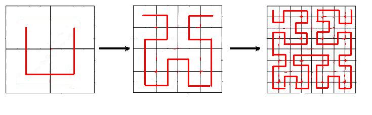
Figure 4: Generation of Hilbert order

These rules can be deduced from the patterns shown in Fig. 3. In turn, Fig. 4 shows the steps of generating the Hilbert order for an $8\times 8$ matrix $M$ of initial pattern $U$. In Fig. 5, the entries of the matrix at the end of the generation of the Hilbert order show the indices of the elements of $M$ within the physical one-dimensional array representing $M$ in the Hilbert order.

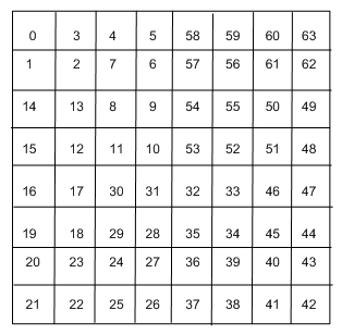
Figure 5: Matrix in the Hilbert Order

The matrix to be laid out in the Hilbert order is given a pattern and refined according to the refinement rules for each pattern. The refinement is done by recursively dividing the matrix into four quadrants and storing them according to the pattern refinement rules. Let $M_{\rho}$ denote a Hilbert matrix of pattern $\rho\in\{U,D,C,N\}$. Each step of the refinement for $M_{\rho}$ is done by identifying the patterns of the quadrants of $M_{\rho}$ and the order in which these quadrants are accessed. This is done using the following structures for each matrix $M_{\rho}$ laid out in some pattern $\rho$:

$$NextPattern(M_{\rho})=\left(\begin{array}[]{cc}\rho_{0}&\rho_{1}\\ \rho_{2}&\rho_{3}\end{array}\right),$$

where $\rho_{i}$ denotes the pattern of the $i^{th}$ quadrant of $M_{\rho}$ in the row-major layout, and

$$HilbertOrder(M_{\rho})=\left(\begin{array}[]{cc}\nu_{0}&\nu_{1}\\ \nu_{2}&\nu_{3}\end{array}\right),$$

where $\nu_{i}$ denotes the index in the Hilbert layout of the $i^{th}$ quadrant of $M_{\rho}$ in the row-major layout.

For example, the refinement rule for the $U$ pattern is given by:

$$NextPattern(U)=\left(\begin{array}[]{cc}D&C\\ U&U\end{array}\right)$$

and

$$HilbertOrder(U)=\left(\begin{array}[]{cc}0&3\\ 1&2\end{array}\right).$$

The refinement process is referred to as the generation of the Hilbert curve and is going to guide the encoding and decoding procedures. Fig. 6 shows an $8\times 8$ matrix stored in the $U$-shaped Hilbert order on which the encoding and decoding procedures will be traced. In the rest of this section, $\Theta$ refers to the Hilbert order and $M$ refers to a $2^{m}\times 2^{m}$ matrix in the Hilbert order.

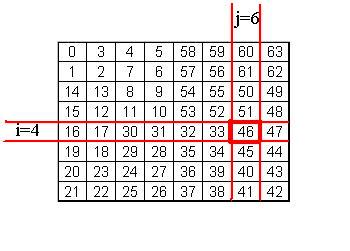
Figure 6: Hilbert Ordered Matrix

3.3.1 Encoding in the Hilbert Order

Given an entry $e$ with Cartesian index $(i,j)$ in the $2^{m}\times 2^{m}$ matrix $M$, we denote by $Q^{k+1}_{e}$ the quadrant of $Q^{k}_{e}$ of dimensions $2^{(m-(k+1))}\times 2^{(m-(k+1))}$ and in which the entry $e$ lies in refinement step $k$, for $k=0,1,..m-1$. We start with $Q^{0}_{e}=M$. To use the refinement rules, we translate them into two lookup tables: Table $\mathcal{T_{P}}$ and Table $\mathcal{T_{V}}$. We index the lookup tables using $\rho$ and $v$: $\rho$ is the pattern of the matrix we are refining and $v$ is the index, in the row-major order, of the quadrant $Q^{k+1}_{e}$ within $Q^{k}_{e}$. Table $\mathcal{T_{P}}$ is a table mapping a pattern $\rho$ and an index $v$ to the next pattern, i.e. the pattern of the block $Q^{k+1}_{e}$, and is given by Table 1. The other look-up table, $\mathcal{T_{V}}$, maps a pattern $\rho$ and an index $v$ to two bits of $z_{\Theta}$ and is given by Table 2. These two bits are the Hilbert index of $Q^{k+1}_{e}$ within $Q^{k}_{e}$.

To determine these tables, consider matrix $M_{\rho}$ of pattern $\rho\in\{U,D,C,N\}$. Let $v\in\{0,1,2,3\}$ refer to the row-major index of any quadrant of $M$, designating $NW$, $NE$, $SW$, and $SE$ respectively. The entry

$$\mathcal{T_{P}}(\rho,v)=\rho^{\prime}$$

is determined as follows: $\rho^{\prime}$ is the pattern of the $v^{th}$ quadrant of $M_{\rho}$ in the row-major order. Table $\mathcal{T_{V}}$ presents a mapping between the row-major layout of the quadrants of a matrix of pattern $\rho$ and the Hilbert layout of these quadrants. The entry

$$\mathcal{T_{V}}(\rho,v)=v^{\prime}$$

is the Hilbert index of the $v^{th}$ quadrant of $M_{\rho}$ in the row-major order.

For example, recall that a matrix of the $U$ Hilbert pattern is refined as follows:

$$NextPattern(M_{U})=\left(\begin{array}[]{cc}D&C\\ U&U\end{array}\right)$$

and

$$HilbertOrder(M_{U})=\left(\begin{array}[]{cc}0&3\\ 1&2\end{array}\right).$$

Hence the entry $\mathcal{T_{P}}(U,1)$ is $C$ and $\mathcal{T_{V}}(U,1)=3=(11)_{2}$.

Recall that $Q^{k}_{e}$ denotes the $2^{(m-k)}\times 2^{(m-k)}$ quadrant of $Q^{k-1}_{e}$ in which the element $e$ of Cartesian index $(i,j)$ lies at each refinement step. Table $\mathcal{T_{P}}$ guides the generation of $z_{\Theta}$ by identifying the pattern of $Q^{k+1}_{e}$. Table $\mathcal{T_{V}}$ identifies two bits to be appended at each iteration to a binary index $z_{k}$. These two bits represent the index, in the Hilbert layout, of $Q^{k+1}_{e}$ within $Q^{k}_{e}$. We justify that this index is identified using two bits as follows. Recall that $Q^{k+1}_{e}$ is one of the quadrants of $Q^{k}_{e}$. There are only four quadrants in a matrix. Hence, the possible values for the index of any of these quadrants - regardless of the layout - are 0, 1, 2, and 3, which can be represented using at most two bits. Hence, the length of the binary representation of this index is at most two.

Table 1: Encoding Pattern Look-Up Table $\mathcal{T_{P}}$

	0	1	2	3
U	$D$	$C$	$U$	$U$
C	$C$	$U$	$C$	$N$
D	$U$	$D$	$N$	$D$
N	$N$	$N$	$D$	$C$

Table 2: Encoding Bits Look-Up Table $\mathcal{T_{V}}$

	0	1	2	3
U	00	11	01	10
C	10	11	01	00
D	00	01	11	10
N	10	01	11	00

Now that the lookup tables are ready, we describe the iterative encoding procedure for a given $2^{m}\times 2^{m}$ matrix and a Cartesian index $(i,j)$. Each iteration represents a refinement step within the generation of the Hilbert curve and, after $m$ iterations, the sequence $\{z_{k+1}\}_{k=0,1,...,m-1}$, converges to $z_{\Theta}$. In each iteration $k$, the pattern $\rho_{k}$ - whether $U$, $C$, $D$, or $N$ - of the quadrant $Q^{k+1}_{e}$ of $Q^{k}_{e}$ must be determined. Recall that $Q^{k}_{e}$ is the $2^{(m-k)}\times 2^{(m-k)}$ sub-block of $M$ containing element $e$ of Cartesian index $(i,j)$. The initial $Q^{0}_{e}$ is $M$ and $\rho_{0}=U$ because the Hilbert pattern we assume for the initial matrix is $U$. The corresponding index in the Hilbert order is progressively calculated by finding some partial index $z_{k}$ in each iteration. The algorithm begins with $z_{0}=0$ and ends with the value for $z_{m}=z_{\Theta}$. Write

$$i=(i_{m-1}...i_{2}i_{1}i_{0})_{2}$$

and

$$j=(j_{m-1}...j_{2}j_{1}j_{0})_{2}.$$

Recall that there are $m$ bits in each of $i$ and $j$, because at most $m$ bits are needed to represent a value between 0 and $2^{m-1}$ in the binary system. In each iteration $k$ of the encoding algorithm:

• we generate an auxiliary index $v_{k}=(i_{(m-1-k)}j_{(m-1-k)})_{2}$, where $v_{k}\in\{0,1,2,3\}$, the two-bit, row-major index of $Q^{k+1}_{e}$ within $Q^{k}_{e}$.

• we use $v_{k}$ and $\rho_{k}$ to index the lookup table $\mathcal{T_{P}}$ and find the next pattern of $Q^{k+1}_{e}$ $\rho_{k+1}=\mathcal{T_{P}}(\rho_{k},v_{k})$.

• we use $v_{k}$ and $\rho_{k}$ to index the lookup table $\mathcal{T_{V}}$ and find

  $$z_{k+1}=(z_{k}<<2)|\mathcal{T_{V}}(\rho_{k},v_{k}).$$

  This appends the two bits of the Hilbert index of $Q^{k+1}_{e}$ within $Q^{k}_{e}$ to the partial index $z_{k}$ to get $z_{k+1}$.

As two bits are appended to $z_{k}$ at each iteration, and there are $m$ iterations, then $z_{\Theta}$ is formed of $2m$ bits.

To prove correctness, we propose the following:

Lemma 3.1

The auxiliary variable $v_{k}$ is the row-major index of $Q^{k+1}_{e}$ within $Q^{k}_{e}$.

proof

Consider the entry $e$ of Cartesian index $(i,j)$. Write

$$i=(i_{m-1}...i_{2}i_{1}i_{0})_{2}$$

and

$$j=(j_{m-1}...j_{2}j_{1}j_{0})_{2}.$$

To prove that $v_{k}$ is the row-major index of $Q^{k+1}_{e}$ within $Q^{k}_{e}$, we will show that the bits $i_{(m-1-k)}$ and $j_{(m-1-k)}$ are the row and column indices of the $Q^{k+1}_{e}$ within $Q^{k}_{e}$ respectively, from which it follows directly that $v_{k}$, the concatenation of $j_{(m-1-k)}$ to $i_{(m-i-k)}$, is the row-major index of $Q^{k+1}_{e}$ within $Q^{k}_{e}$. We proceed by induction on $k$.

Base Case: For $k=0$, recall that $Q^{0}_{e}$ is the $2^{m}\times 2^{m}$ matrix $M$. Let $i_{B}$ denote the row index of $Q^{1}_{e}$ within $Q^{0}_{e}$. We need to show that $i_{B}=i_{(m-1)}$. Let $i_{r}$ denote the row index of $e$ within $Q^{1}_{e}$. The row index $i$ of $e$ is given by $i=i_{B}\times 2^{m-1}+i_{r}$ since $Q^{1}_{e}$ is of size $2^{m-1}\times 2^{m-1}$. The equation $i=i_{B}\times 2^{m-1}+i_{r}$ is equivalent to

$$i=(i_{B}<<(m-1))|i_{r}$$

in bit operations . Hence, $i_{B}$ is the $(m-1)^{st}$ bit of $i$ given by $i_{(m-1)}$. This establishes the base case.

Induction Step: We want to show that $i_{(m-(k+1))}$ is the row index of $Q^{k+1}_{e}$ within $Q^{k}_{e}$. Let $i_{B}$ denote the row index of $Q^{k+1}_{e}$ within $Q^{k}_{e}$. We need to show that $i_{B}=i_{(m-(k+1))}$. Let $i_{r}$ and $i^{\prime}_{r}$ denote the row index of $e$ within $Q^{k}_{e}$ and $Q^{k+1}_{e}$ respectively. As $Q^{k+1}_{e}$ is a $2^{m-(k+1)}\times 2^{m-(k+1)}$ quadrant within $Q^{k}_{e}$, we have

$$i_{r}=i_{B}\times 2^{m-(k+1)}+i^{\prime}_{r}$$

which is equivalent to

$$i_{r}=(i_{B}<<(m-(k+1)))|i^{\prime}_{r}.$$ (5)

By induction, we know that the bit $i_{(m-1-k)}$ is the row index of $Q^{k}_{e}$ within $Q^{k-1}_{e}$, so that

$$i=(i_{m-1}i_{m-2}...i_{(m-k)}<<(m-k))|i_{r}.$$ (6)

Replacing $i_{r}$ as in Eq. (5) in Eq. (6) above, we obtain

$$i=(i_{m-1}i_{m-2}...i_{(m-k)}<<(m-k))|(i_{B}<<(m-(k+1)))|i^{\prime}_{r}.$$

Hence the $i_{(m-(k+1))}=_{B}$. This establishes the induction step and concludes the proof.

Proposition 3.2

The partial index $z_{k}$ is the Hilbert index of the sub-block $Q^{k}_{e}$ of dimenions $2^{(m-k)}\times 2^{(m-k)}$ within $M$, for $k=0,1,...m$.

proof

We proceed by induction on $k$.

Base Case: For $k=0$, $Q^{k}_{e}\equiv M$ and has index $z_{k}=z_{0}=0$ within the Hilbert layout of $M$.

Induction Step: We assume that $z_{k}$ is the Hilbert index of the $2^{(m-k)}\times 2^{(m-k)}$ sub-block $Q^{k}_{e}$ within $M$. We refine more and obtain the $2^{(m-(k+1))}\times 2^{(m-(k+1))}$ quadrant $Q^{k+1}_{e}$ within $Q^{k}_{e}$. From Prop. 3.1, we know that $v_{k}$ is the row-major index of $Q^{k+1}_{e}$ within $Q^{k}_{e}$. The quadrant $Q^{k+1}_{e}$ has Hilbert index $v^{\prime}_{k}=\mathcal{T_{V}}(\rho_{k},v_{k})$ within $Q^{k}_{e}$ from the definition of table $\mathcal{T_{V}}$. We will show that

$$z_{k+1}=(z_{k}<<2)|v^{\prime}_{k}$$

is the Hilbert index of $Q^{k+1}_{e}$ within $M$. By induction, $z_{k}$ represents the Hilbert index of $Q^{k}_{e}$ within $M$. Upon another refinement step, each of the $2^{(m-k)}\times 2^{(m-k)}$ sub-blocks of $M$ is in turn divided into four quadrants of size $2^{(m-(k+1))}\times 2^{(m-(k+1))}$ each. The indices of the four quadrants of $Q^{k}_{e}$ are obtained by $z_{k}\times 4$, $z_{k}\times 4+1$, $z_{k}\times 4+2$, and $z_{k}\times 4+3$ depending on their index $v^{\prime}_{k}$ in the Hilbert layout of $Q^{k}_{e}$. These indices can be re-written as $(z_{k}<<2)|00$, $(z_{k}<<2)|01$, $(z_{k}<<2)|10$, and $(z_{k}<<2)|11$. The sub-block $Q^{k+1}_{e}$ is a quadrant of $Q^{k}_{e}$ and thus $Q^{k+1}_{e}$ takes on one of these indices depending on its Hilbert index $v^{\prime}_{k}$ within $Q^{k}_{e}$. Thus $Q^{k+1}_{e}$ has index

$$z_{k+1}=(z_{k}<<2)|v^{\prime}_{k}$$

within $M$. This concludes the proof.

Corollary 3.3

The index $z_{m}$ is $z_{\Theta}$.

proof

For $k=m$, $z_{m}$ is the Hilbert index of the smallest sub-block $Q^{m}_{e}$ within $M$ containing $e$, which is $e$ itself. This concludes the proof.

We illustrate this encoding procedure with an example in Appendix A.

3.3.2 Decoding in the Hilbert Order

In the decoding procedure, we are given the Hilbert index $z_{\Theta}$ of an entry $e$ and we wish to find $(i,j)$, the Cartesian index of $e$. Recall that $Q^{k}_{e}$ denotes the quadrant of $Q^{k-1}_{e}$ in which $e$ lies, starting with $Q^{0}_{e}=M$. To find $(i,j)$, we need two different lookup tables: $\mathcal{T^{\prime}_{P}}$ (Table 3 below) is used to identify the pattern of $Q^{k}_{e}$. Table $\mathcal{T^{\prime}_{V}}$ (Table 4 below) is used to find a two-bit value $v^{\prime}_{k}$ representing the row-major index of $Q^{k}_{e}$ within $Q^{k-1}_{e}$. To determine these tables, consider matrix $M_{\rho}$ of pattern $\rho\in\{U,D,C,N\}$. Recall that the $NW$, $NE$, $SW$, and $SE$ quadrants are the $0^{th}$, $1^{st}$, $2^{nd}$, $3^{rd}$ quadrants in the row-major order. Entries in Table $\mathcal{T^{\prime}_{P}}$ represent patterns and are given by:

$$\mathcal{T^{\prime}_{P}}(\rho,v)=\rho^{\prime}.$$

The pattern $\rho^{\prime}$ refers to the pattern of the $v^{th}$ quadrant of $M_{\rho}$ in the Hilbert order. Table $\mathcal{T^{\prime}_{V}}$ presents a mapping between the Hilbert layout of the quadrants of $M_{\rho}$ and the row-major layout of these quadrants. The entry

$$\mathcal{T^{\prime}_{V}}(\rho,v)=v^{\prime}$$

indicates that the $v^{th}$ quadrant of $M_{\rho}$ in the Hilbert order is the $v^{\prime th}$ quadrant of $M_{\rho}$ in the row-major order. Note that $\mathcal{T^{\prime}_{V}}$ is the inverse mapping of the table $\mathcal{T_{V}}$ used for encoding: i.e.

$$\mathcal{T^{\prime}_{V}}(\rho,v)=v^{\prime}\leftrightarrow\mathcal{T_{V}}(\rho,v^{\prime})=v.$$

For example, recall that a matrix $M_{U}$ in a $U$ Hilbert pattern is refined as follows:

$$NextPattern(M_{U})=\left(\begin{array}[]{cc}D&C\\ U&U\end{array}\right),$$

and

$$HilbertOrder(M_{U})=\left(\begin{array}[]{cc}0&3\\ 1&2\end{array}\right).$$

Hence, we have $\mathcal{T^{\prime}_{P}}(U,3)=C$ because the $3^{rd}$ quadrant of $M_{U}$ in the Hilbert order has pattern $C$. Also, $\mathcal{T^{\prime}_{V}}(U,3)=1=(01)_{2}$ because the $3^{rd}$ quadrant of $M_{U}$ in the Hilbert order is the $1^{st}$ - i.e. the $NE$ quadrant of $M_{U}$ in the row-major order. Tables $\mathcal{T^{\prime}_{P}}$ and $\mathcal{T^{\prime}_{V}}$ guide the generation of $i$ and $j$ by identifying the pattern of $Q^{k}_{e}$ and the row-major index of $Q^{k}_{e}$ within $M$ respectively.

Table 3: Decoding Pattern Look-Up Table $\mathcal{T^{\prime}_{P}}$

	0	1	2	3
U	$D$	$U$	$U$	$C$
C	$N$	$C$	$C$	$U$
D	$U$	$D$	$D$	$N$
N	$C$	$N$	$N$	$D$

Table 4: Decoding Bits Look-Up Table $\mathcal{T^{\prime}_{V}}$

	0	1	2	3
U	00	10	11	01
C	11	10	00	01
D	00	01	10	11
N	11	01	00	10

Now that the lookup tables have been described, we present the decoding procedure. Recall from the encoding procedure that $z_{\Theta}$ is formed of $2m$ bits. Write

$$z_{\Theta}=(z_{2m-1}...z_{2}z_{1}z_{0})_{2}.$$

The decoding reverses the encoding procedure, in which at each iteration one bit of each of $i$ and $j$ is used to generate two bits of $z$. Recall, from encoding, that, in each iteration $k$, these two bits of $z_{\Theta}$ make up the Hilbert index of $Q^{k}_{e}$ within $Q^{k-1}_{e}$ as follows:

$$v_{k}=(z_{(2m-1-2k)}z_{(2m-1-(2k+1))})_{2}.$$

Also, we identify the pattern $\rho_{k}$ of $Q^{k}_{e}$. We start with $\rho_{0}=U$. In each iteration $k$, $\rho_{k}$ and $v_{k}$ are used to index the two lookup tables $\mathcal{T^{\prime}_{P}}$ and $\mathcal{T^{\prime}_{V}}$. As mentioned earlier, table $\mathcal{T^{\prime}_{P}}$ is used to find the pattern of the quadrant of the next iteration $Q^{k+1}_{e}$, given by $\rho_{k+1}=\mathcal{T^{\prime}_{P}}(\rho_{k},v_{k})$. Table $\mathcal{T^{\prime}_{V}}$ is used to find a two-bit value $v^{\prime}_{k}=(b_{i}b_{j})_{2}$ which represents the row-major index of $Q^{k+1}_{e}$ within $Q^{k}_{e}$. Recall that this is a two-bit value because it represents the index of a quadrant. The values of $i$ and $j$ are found progressively: start with $i_{0}=0$ and $j_{0}=0$. In each iteration append $b_{i}\in\{0,1\}$ and $b_{j}\in\{0,1\}$ to $i_{k}$ and $j_{k}$ to get $i_{k+1}$ and $j_{k+1}$ respectively. In bit operations, this corresponds to

$$i_{k+1}=(i_{k}<<1)|(v^{\prime}_{k}>>1),$$

appends bit $b_{i}$ to $i_{k}$ to get $i_{k+1}$, and

$$j_{k+1}=(j_{k}<<1)|(v^{\prime}_{k}\&1),$$

which appends bit $b_{j}$ to $j_{k}$ to get $j_{k+1}$. This reverses the process of encoding. We iterate $m$ times, after which we have $i_{m}=i$ and $j_{m}=j$.

We illustrate this decoding procedure with an example in Appendix B.

3.3.3 Computation Overhead

Each of encoding and decoding requires $m$ iterations. In each iteration, the encoding operation uses six bit operations and two table look-ups and the decoding algorithm uses eight bit operations and two table look-ups. The first of each table look-up incurs a random cache miss. The tables are small enough to fit in internal memory. As row and column permutations swaps in TURBO take place consecutively in one batch, so do the conversion routines, each of which requires access to the look-up table. By the LRU cache policy, the tables are kept in internal memory until the permutations have concluded. Consequently, the overall I/O cost for table lookups is $\Theta(1)$ per one batch of permutations, which is dominated by the I/O cost of the matrix operations in each recursive step, and hence, can be discarded. Summarising, the overall run-time for each of encoding and decoding in the Hilbert order is $\Theta(m)$ bit operations.

Algorithms for encoding and decoding in the Hilbert order which do not use look-up tables are described in full detail in [15]. In [10], a new variant of the Hilbert curve is introduced for which the encoding runtime overhead is $O(\lg(\max(i,j)))$. Yet, such conversion schemes are still beaten by the Morton and Morton-hybrid layouts as we will describe in Sec. 3.5 and Sec. 3.6 respectively.

3.4 Encoding/Decoding in the Peano Layout

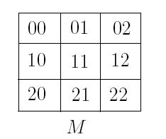
Figure 7: Peano Matrix Division

The Peano ordering of a matrix is based on the Peano space filling curve. This ordering results from recursive construction and assumes the matrix has dimension $3^{m}\times 3^{m}$ [5]. Each dimension of $M$ is divided into $3$ equal parts as shown in Fig. 7 resulting in nine sub-matrices which are named $\{00,01,02,10,11,12,20,21,22\}$. The Peano order for each of the resulting sub-matrices is recursively generated according to a certain precedence depending on the pattern of the higher level sub-matrix.

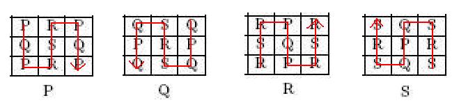
Figure 8: Peano Generation Rules

Any Peano sub-matrix has a pattern from the set of primitive patterns $\{P,Q,R,S\}$ shown in Fig. 8. The Peano order assumes the initial matrix $M$ has pattern $P$. We denote by $Q^{k}$ the sub-matrix we are laying onto memory for each recursive level and denote by $\rho_{Q^{k}}$ the pattern of the sub-matrix $Q^{k}$ obtained from the set $\{P,Q,R,S\}$. We start with $Q^{0}=M$ of pattern $\rho_{Q^{0}}=P$. At the $k^{th}$ step, each of the sub-matrices $Q^{k}$ is refined into nine quadrants $Q^{k+1}\in\{00_{Q^{k}},01_{Q^{k}},02_{Q^{k}},10_{Q^{k}},11_{Q^{k}},12_{Q^{k}},20_{Q^{k}},21_{Q^{k}},22_{Q^{k}}\}$ of $Q^{k}$. These are then laid onto memory in the Peano order governed by two rules: the $NextPattern$ rule and the $PeanoOrder$ rule, similar to the rules governing the generation of the Hilbert order. Let $M_{\rho}$ denote any matrix $M$ of pattern $\rho\in\{P,Q,R,S\}$. Let $i\in\{0,1,2,3,4,5,6,7,8\}$ denote the sub-matrices of $M_{\rho}$ where each $i$ refers to the $00$, $01$, $02$, $10$, $11$, $12$, $20$, $21$, and $22$ sub-matrices respectively. The $NextPattern(M_{\rho})$ rule for any sub-matrix $M$ of pattern $\rho_{M}\in\{P,Q,R,S\}$ identifies the pattern of each quadrant of $M$. The $PeanoOrder(M_{\rho})$ rule identifies the order of precedence in which these quadrants are mapped onto memory. These rules can also be seen from Fig. 8: the precedence order of the sub-matrices is given by the direction of the arrow and the pattern is given by the letter inside the sub-matrix.

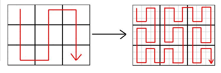
Figure 9: Generation of Peano order

Fig. 9 shows the steps for the generation of the Peano order for a $9\times 9$ matrix $M$. In Fig. 10, the entries of the matrix at the end of the generation of the Peano order show the indices of the elements of $M$ within the physical one-dimensional array representing $M$ in the Peano order.

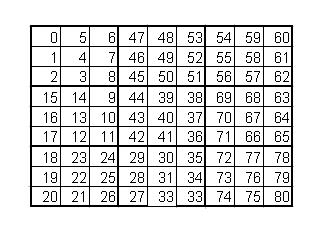
Figure 10: Matrix in the Peano Order

The Peano-based ordering of matrices has the property that computations within matrix-matrix multiplication can be re-ordered so as to ensure no jumps in the address space [5].

The Peano layout is similar to the Hilbert layout in that it is based on more than one pattern, and so the encoding and decoding procedures for the Peano layout are analogous to those for the Hilbert layout. Specifically, the indices are encoded (or decoded) progressively through iterations. In each iteration, a pattern identifier is used along with a set of lookup tables to identify auxiliary variables for the next iteration. The differences between the procedure for the Peano layout and those for the Hilbert layout are:

• The operations used in each iteration are operations in base 3 - division by 3 and modulo 3.

• The resulting indices are in base 3 and need to be converted to base 2.

This results in $m$ iterations with a constant number of operations in base 3 per iteration, which cannot be replaced by bit operations. Conversion between base 3 and base 2 values is also needed at the end of the iterative computations in order to get the final indices. In total, this makes encoding and decoding indices within the Peano layout significantly costly as opposed to the Hilbert, Morton, and Morton-hybrid orders. As such, we rule out using the Peano order within the TURBO algorithm. This is specifically so because the nature of the recursive TU decomposition algorithms requires row-wise and column-wise traversal of the matrix for pivoting and permutations – in contrast to matrix multiplication where any traversal that suits the layout may be used.

3.5 Encoding/Decoding in the Morton Layout

The Morton order is another alternative layout used for $2^{m}\times 2^{m}$ matrices. To generate the Morton-order of a matrix, the latter is divided into four quadrants, which are laid out onto memory in the order northwest, northeast, southwest, then southeast. The Morton order differs from the Hilbert order in that it does not alternate between patterns, but rather uses the same pattern to generate the Morton order for each of the sub-matrices. In this section, we present the $Z$-shaped Morton order, in which the pattern used looks like the letter Z as can be seen in Fig. 11.

Figure 11: Morton $Z$ Pattern

Fig. 12 shows the steps in the generation of the $Z$-shaped Morton order of an $8\times 8$ matrix. For this example, there are three levels of decomposition, after which the entries of the matrix are laid out as shown in Fig. 13.

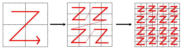
Figure 12: Generation of Morton order

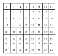
Figure 13: Matrix in Morton Order

In the remainder of this section, $\Theta$ refers to the Morton layout and we assume a given matrix $M$ of dimensions $2^{m}\times 2^{m}$. Given a Cartesian index $(i,j)$, recall that the length of the binary representation of $i$ and $j$ is at most $m$ because $i,j\in\{0,1,2,...,2^{m}-1\}$. These values can be represented by at most $m$ bits. Write

$$i=(i_{m-1}...i_{4}i_{3}i_{2}i_{1}i_{0})_{2}$$

and

$$j=(j_{m-1}...j_{4}j_{3}j_{2}j_{1}j_{0})_{2}.$$

According to [16], the corresponding Morton index $z_{\Theta}$ is

$$z_{\Theta}=(i_{m-1}j_{m-1}...i_{4}j_{4}i_{3}j_{3}i_{2}j_{2}i_{1}j_{1}i_{0}j_{0})_{2},$$ (7)

which represents an inter-leaving of the bits of $i$ and $j$. The reverse process by which we extract the bits of $i$ and $j$ from the bits of $z_{\Theta}$ is referred to as de-leaving. In this section, we derive the costs for encoding and decoding the Morton order based on this inter-leaving of indices. For this, we revisit the notions of dilating and un-dilating integers from [16]. Dilating an integer $k=(k_{b-1}...k_{4}k_{3}k_{2}k_{1}k_{0})_{2}$ of $b$ bits is the process of expanding $k$ into an integer $k^{\prime}=(0k_{b-1}...0k_{4}0k_{3}0k_{2}0k_{1}0k_{0})_{2}$ of $2\times b$ bits by inserting a zero bit between every two bits of $k$. Un-dilating is the reverse process that takes $k^{\prime}$ back to $k$. Before we determine the computational overhead for index conversion, we review here two algorithms - dilate and un-dilate - that perform the encoding and decoding between Morton order indices and Cartesian indices. Fig. 14 shows an $8\times 8$ Morton ordered matrix on which the encoding and decoding procedures will be traced.

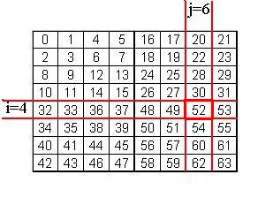
Figure 14: Morton Ordered Matrix

3.5.1 Encoding in the Morton Order

1unsigned int $r$ = $t$

2 $r$ = ($r$ $|$ ($r$ $<<$ 8)) & $0$x$00FF00FF$

3 $r$ = ($r$ $|$ ($r$ $<<$ 4)) & $0$x$0F0F0F0F$

4 $r$ = ($r$ $|$ ($r$ $<<$ 2)) & $0$x$33333333$

5 $r$ = ($r$ $|$ ($r$ $<<$ 1)) & $0$x$55555555$

6 return $r$

Algorithm 3 (unsigned int) dilate( unsigned short t) [20]

All the present discussion follows from [16, 20]. For encoding the Morton order, $z_{\Theta}$ must be found given $(i,j)$. As shown in Eq. (7), the inter-leaving of the bits of $i$ and $j$ must be performed. This can be done by finding the dilated forms of $i$ and $j$, denoted by $i^{\prime}$ and $j^{\prime}$ respectively. The algorithm for dilation is given by Alg. 3 from [20]. According to the definition of dilation above, dilating $i$ and $j$ gives

$$i^{\prime}=(0i_{m-1}0i_{m-2}...0i_{3}0i_{2}0i_{1}0i_{0})_{2}$$

and

$$j^{\prime}=(0j_{m-1}0j_{m-2}...0j_{3}0j_{2}0j_{1}0j_{0})_{2}.$$

Then $z_{\Theta}$ is given by

$$z_{\Theta}=(i^{\prime}<<1)|j^{\prime}.$$ (8)

To verify Eq. (8) from [16], perform

$$i^{\prime}<<1=(i_{m-1}0i_{m-2}0...i_{3}0i_{2}0i_{1}0i_{0}0)_{2}$$

followed by

$$(i^{\prime}<<1)|j^{\prime}=(i_{m-1}j_{m-1}i_{m-2}j_{m-2}...i_{3}j_{3}i_{2}j_{2}i_{1}j_{1}i_{0}j_{0})_{2}.$$

We illustrate this encoding procedure with an example in Appendix C.

3.5.2 Decoding in the Morton Order

To decode the Morton order, we need to extract $i$ and $j$ from $z_{\Theta}$. We write $z_{\Theta}$ as in Eq. (7). Then, the bits of $z_{\Theta}$ must be de-leaved to separate the bits of $i$, denoted $i_{z_{\Theta}}$, from the bits of $j$, denoted $j_{z_{\Theta}}$. To do this, we mask $z_{\Theta}$ with $0$x$AAAAAAAA$ to get

$$i_{z_{\Theta}}=(i_{m-1}0i_{m-2}0...i_{3}0i_{2}0i_{1}0i_{0}0)_{2}.$$

and mask $z_{\Theta}$ with $0$x$55555555$ to get

$$j_{z_{\Theta}}=(0j_{m-1}0j_{m-2}...0j_{3}0j_{2}0j_{1}0j_{0})_{2}.$$

Now we shift $i_{z_{\Theta}}$ one position to the right to get

$$i^{\prime}_{z_{\Theta}}=i_{z_{\Theta}}>>1=(0i_{m-1}0i_{m-2}...0i_{3}0i_{2}0i_{1}0i_{0})_{2}.$$

To calculate $i$, we un-dilate $i^{\prime}_{z_{\Theta}}$ using the un-dilation algorithm given in Alg. 4. To calculate $j$, we un-dilate $j_{z_{\Theta}}$ using Alg. 4.

1unsigned int $r$ = $t$

2 $t$ = ($t$ $|$ ($t$ $>>$ 1)) & $0$x$33333333$

3 $t$ = ($t$ $|$ ($t$ $>>$ 2)) & $0$x$0F0F0F0F$

4 $t$ = ($t$ $|$ ($t$ $>>$ 4)) & $0$x$00FF00FF$

5 $t$ = ($t$ $|$ ($t$ $>>$ 8)) & $0$x$0000FFFF$

6 return (unsigned short)$t$

Algorithm 4 unsigned short un-dilate( unsigned int t) taken from [16, 20]

We illustrate this decoding procedure with an example in Appendix D.

3.5.3 Computation Overhead

Assume that the input matrix has dimensions $2^{\alpha}\times 2^{\alpha}$, where $\alpha$ is the machine word-size. This guarantees that each cartesian index fits in a machine word. For the typical value $\alpha=64$, such matrix sizes are very generous. Each of dilation and un-dilation performs twelve bit operations: four OR operations, four AND operations, and four bit-shift operations. The encoding procedure makes use of the dilation algorithm twice, followed by one bit-shift operation and one OR operation. This results in a total of twenty six bit operations for encoding an index in the Morton order. The decoding procedure makes use of two masking operations, one bit-shift operation, and two calls to the un-dilation algorithm: one for un-dilating $i_{z}$ and one for un-dilating $j_{z}$. This requires a total of twenty seven bit operations for decoding a Morton index to a Cartesian index.

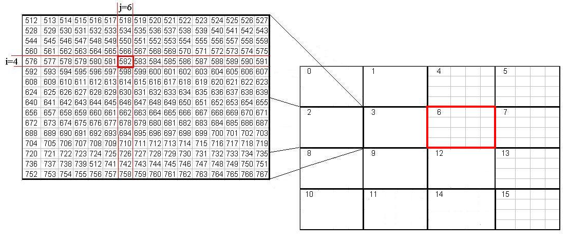
Figure 15: Morton-Hybrid Ordered Matrix with $T=16$

3.6 Encoding/Decoding in the Morton-Hybrid Layout

The Morton-hybrid order is a variant of the Morton order used in [2] and [8] among others. In this variant of the Morton order, the recursive sub-dividing into blocks stops at a given truncation size $T$, resulting in a base case block of size $T\times T$, for which the row-major order is used. The value of the truncation size can vary.

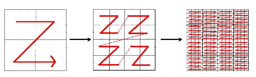
Figure 16: Generation of Morton-hybrid order

To generate the Morton-hybrid order, the procedure for generation of the Morton order is followed, using the $Z$ pattern as shown in Fig. 11, until the size of the sub-matrix being mapped onto memory is $T\times T$. To map the entries of this block in the one-dimensional array representing the matrix, a row-major order is assumed. Fig. 16 shows the steps in the generation of the $Z$-shaped Morton-hybrid order of an $16\times 16$ matrix for truncation size $T=4$. The resulting map of the entries of the matrix in the corresponding one-dimensional array in memory can be seen in Fig. 17.

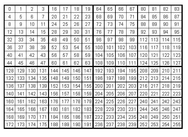
Figure 17: Matrix in Morton-hybrid Order

The following presentation of the Morton-hybrid index for $T=16$ was taken from [2], but we elaborate on it additionally in our Proposition 3.4 below and the associated proof. For the remainder of this section, $\Theta$ denotes the Morton-hybrid layout for $T=16$. We assume the input matrix $M$ has dimension $2^{m}\times 2^{m}$. In Sec. 3.5, we saw that the Morton index is determined using the inter-leaving of the bits of $i$ and $j$, for a given Cartesian index $(i,j)$. In Sec. 3.2 the row major index was composed of the bits of $j$ concatenated to the bits of $i$. The Morton-hybrid order is a combination of both these orders.

Consider the Morton-hybrid matrix shown in Fig. 15 showing row-major sub-blocks of a Morton-hybrid matrix for $T=16$. Each $16\times 16$ row-major block has a row index and a column index as given in Sec. 3.1. For example, consider the row-major sub-block outlined in red in Fig. 15. Its row index is 1 and its column index is 2. The Morton index of a sub-block in the Morton-hybrid order is then given by the interleaving of the block row and block column indices as per the Morton indexing scheme. Now, each entry $e$ in a Morton-hybrid matrix can be indexed with the help of information regarding:

1. the $T\times T$ row-major sub-block in which it lies

2. its row index within this row-major sub-block

3. its column index within this row-major sub-block

For each element $e$ in a $T\times T$ sub-block, the possible values for the row and column indices of $e$ within this block can be 0, 1, …, $T-1$. Thus, the offset values can be represented using $\beta$ bits where $T=2^{\beta}$. Let $(i,j)$ denote the Cartesian index of $e$. We now have:

Proposition 3.4

The $\beta$ lower order bits of $i$ represent the row index of the element within the $T\times T$ row-major sub-block and the $(m-\beta)$ higher order bits of $i$ represent the row index of this $T\times T$ sub-block.

proof

Let $M$ be a $2^{m}\times 2^{m}$ matrix laid out in the Morton-hybrid order with truncation size $T=2^{\beta}$. Let $e$ be any entry in the $T\times T$ row-major sub-block $S_{M}$ of $M$, and let $(i,j)$ denote the Cartesian index of $e$. First we show that the bit representations of the row index of the sub-block $S_{M}$ and the row index of the element $e$ within $S_{M}$ require $(m-\beta)$ and $\beta$ bits respectively.

The matrix $M$ has dimensions $2^{m}\times 2^{m}$ and the sub-blocks at the base case have dimensions $T\times T$, with $T=2^{\beta}$. Thus there are exactly $2^{(m-\beta)}$ rows of $T\times T$ blocks and the row index $i_{M}$ of a sub-block can be 0, 1,…, $2^{(m-\beta)}-1$. So these row indices require $(m-\beta)$ bits to be represented. The $T\times T$ sub-block $S_{M}$ of $M$ is in the row-major layout and contains $T$ rows of entries. Let $r$ denote the row of $S_{M}$ in which entry $e$ lies. The row index $i_{r}$ of $e$ within $S_{M}$, which is the same as the row index of any entry within $r$, can be $0$, $1$,$\ldots$, $T-1$ and thus its bit representation requires $\beta$ bits.

Now we identify where to get these bits from. The row index $i$ of the entry $e$ within $M$ is given by

$$i=i_{M}\times T+i_{r}$$

which is equivalent to

$$i=(i_{M}<<\beta)|i_{r}.$$

As such, $i$ can be represented by $m$ bits: the higher order $(m-\beta)$ bits are the bits of $i_{M}$, making up the row index of $S_{M}$ within $M$, and the $\beta$ lower order bits are the bits of $i_{r}$, making up the row index of $e$ within $S_{M}$. This concludes the proof.

To illustrate the proposition, take for example the element $(20,6)$ from Fig. 15. In this example, $n=2^{m}=64$, i.e. $m=6$, and $T=2^{\beta}=16$, so $\beta=4$. Consider $i=20=(010100)_{2}$. The $\beta=4$ lower order bits are $(0100)_{2}=4$, the element’s row index within the row-major block, $i_{r}$. The $m-\beta=2$ higher order bits $(01)_{2}=2$ identify the row index of the row-major sub-block in which this element lies. The same applies to $j=6=(000110)_{2}$. The $\beta=4$ lower order bits $(0110)_{2}=6$ are the column index of the element within the row-major block. The $m-\beta=2$ higher order bits, $(00)_{2}$, correspond to the column index of the block.

Now consider a matrix $M$ laid out in the Morton-hybrid order and an entry $e$ in $M$. Let $z_{\Theta}$ denote the Morton-hybrid index of $e$ and $(i,j)$ denote its Cartesian index. Let $S_{M}$ denote the $T\times T$ row-major sub-block in which $e$ lies. Recall the interleaving of the two coordinates $i$ and $j$ presented in Sec. 3.5 leading up to the Morton index of $e$. The $T\times T$ sub-blocks of $M$ are laid out in the Morton order, so we use this procedure to inter-leave the $(m-\beta)$ higher order bits of $i$ and $j$ to get the Morton index $z_{M}$ of $S_{M}$. Then, we find the row-major index of $e$ within $S_{M}$: as $S_{M}$ is stored in row-major order, the index within $S_{M}$ of $e$ is in the context of a row-major ordering scheme. To get the row-major index of $e$ within $S_{M}$, denoted by $z_{r}$, we concatenate $j_{r}$ to $i_{r}$, where $i_{r}$ and $j_{r}$ are the row and column indices of element $e$ within $S_{M}$ respectively (according to Sec. 3.2). Because the smallest sub-blocks of $M$ are of size $T\times T$, the Morton-hybrid index of the element $e$ of Cartesian index $(i,j)$ is then given by

$$(z_{M}\times T^{2})+z_{r}$$

or

$$(z_{M}<<2\cdot\beta)|z_{r}.$$

Hence, it can be formed by concatenating the row-major offset of $e$ within $S_{M}$ to the Morton index of $S_{M}$ within $M$. Recall, from Prop. 3.4, that the $(m-\beta)$ higher order bits of $i$ and $j$ are row and column indices of $S_{M}$ within $M$ respectively and the $\beta$ lower order bits of $i$ and $j$ are the row and column indices of $e$ within $S_{M}$. That is, if we write

$$i=(i_{m-1}i_{m-2}...i_{\beta}i_{\beta-1}i_{\beta-2}...i_{1}i_{0})_{2}$$

and

$$j=(j_{m-1}j_{m-2}...j_{\beta}j_{\beta-1}j_{\beta-2}...j_{1}j_{0})_{2},$$

the Morton-hybrid index $z_{\Theta}$ is given by

$$z_{\Theta}=(i_{m-1}j_{m-1}i_{m-2}j_{m-2}...i_{\beta+1}j{\beta+1}i_{\beta}j_{\beta}i_{\beta-1}i_{\beta-2}...i_{1}i_{0}j_{\beta-1}j_{\beta-2}...j_{1}j_{0})_{2}.$$

Figure 18: Morton-Hybrid Ordered Matrix with $T=16$

3.6.1 Encoding in the Morton-Hybrid Order

To encode a Cartesian index $(i,j)$ in the Morton-hybrid order, we proceed as follows. The last $\beta$ bits of $i$ must be extracted. To do this, mask $i$ with

$$\mu=(1<<\beta)-1$$

to extract $i_{r}$, the part of the binary representation of $i$ representing the row offset of the element within the row-major block. Thus

$$i_{r}=i\&\mu=(i_{\beta-1}i_{\beta-2}...i_{1}i_{0})_{2}.$$

The rest of $i$ is denoted by $i_{m}$. It represents the row index of the row-major block in which the element $(i,j)$ lies. The value of $i_{m}$ is given by

$$i_{m}=i\&(0xFFFFFFFF<<\beta)=(i_{m-1}...i_{\beta+1}i_{\beta}0000..)_{2}.$$

We find

$$j_{r}=(j_{\beta-1}j_{\beta-2}...j_{1}j_{0})_{2}$$

and

$$j_{m}=(j_{m-1}...j_{\beta+1}j_{\beta}0000..)_{2},$$

the row-major and Morton parts of the index $j$ respectively in a similar manner. The values $j_{r}$ and $j_{m}$ are the column offset of the element in the row-major block and the column index of this block respectively. The Morton-hybrid index $z_{\Theta}$ is found by dilating $i_{m}$ and $j_{m}$ into

$$i^{\prime}_{m}=(0i_{m-1}...0i_{\beta+1}0i_{\beta}00000000)_{2}$$

and

$$j^{\prime}_{m}=(0j_{m-1}...0j_{\beta+1}0j_{\beta}00000000)_{2}$$

respectively using Alg. 3. Then, $z_{\Theta}$ is given by:

$$z_{\Theta}=((i^{\prime}_{m}<<1)|j^{\prime}_{m})|(i_{r}<<\beta)|j_{r}.$$ (9)

Note that this equation is in fact made of two parts:

$$(i^{\prime}_{m}<<1)|j^{\prime}_{m},$$

which performs the interleaving of the Morton parts of the indices as from Eq. (8) from Sec. 3.5 and

$$(i_{r}<<\beta)|j_{r}$$

which appends the row-major parts of the indices as from Alg. 1 from Sec. 3.2 with $m=\beta$.

To verify that this results in $z_{\Theta}$ given in Eq. (3.6), we perform:

$$(i^{\prime}_{m}<<1)=(i_{m-1}0...i_{\beta+1}0i_{\beta}00...00)_{2},$$

$$j^{\prime}_{m}=(0j_{m-1}...0j_{\beta+1}0j_{\beta}00...00)_{2},$$

$$(i_{r}<<\beta)=(i_{\beta-1}i_{\beta-2}...i_{1}i_{0}0...0)_{2},$$

and

$$j_{r}=(j_{\beta-1}j_{\beta-2}...j_{1}j_{0})_{2}.$$

We perform OR operations on the above values to get

$$z_{\Theta}=(i_{m-1}j_{m-1}...i_{\beta+1}j_{\beta+1}i_{\beta}j_{\beta}i_{\beta-1}i_{\beta-2}...i_{1}i_{0}j_{\beta-1}j_{\beta-2}...j_{1}j_{0})_{2}$$

as in Eq. (3.6).

We illustrate this encoding procedure with an example in Appendix E.

3.6.2 Decoding in the Morton-Hybrid Order

When decoding an index in the Morton-hybrid order, we start with

$$z_{\Theta}=(i_{m-1}j_{m-1}...i_{\beta+1}j_{\beta+1}i_{\beta}j_{\beta}i_{\beta-1}i_{\beta-2}...i_{1}i_{0}j_{\beta-1}j_{\beta-2}...j_{1}j_{0})_{2}$$

We wish to find the Cartesian index $(i,j)$ by isolating the bits of $i$ and the bits of $j$. Recall that $z_{\Theta}$ is in fact made of three parts as described in the introduction of this section:

1. the Morton index of the row-major block in which this element lies

2. the row offset of the element within this block

3. the column offset of the element within this block

Thus to determine $i$, the Morton index of the row-major block must be decoded to get a row index, and the row offset of the element within the block is concatenated to this to get $i$. The same applies for $j$.

We extract the two parts for $i$ and $j$ from above as follows, in a reverse process to encoding. Recall from the encoding procedure the intermediate values $i_{r}$, $i_{m}$, $i^{\prime}_{m}$, $j_{r}$, and $j_{m}$. We mask $z_{\Theta}$ by

$$((0xAAAAAAAA<<\beta)<<\beta)$$

to get $i^{\prime}_{m}$ and mask $z_{\Theta}$ by

$$((0x55555555<<\beta)<<\beta)$$

to get $j^{\prime}_{m}$. The result is

$$i^{\prime}_{m}=(i_{m-1}0...i_{\beta+1}0i_{\beta}000....00)_{2}$$

and

$$j^{\prime}_{m}=(0j_{m-1}...0j_{\beta+1}0j_{\beta}00...00)_{2}.$$

Then, $(i^{\prime}_{m}>>1)$ and $j^{\prime}_{m}$ are un-dilated using Alg. 4 to get

$$i_{m}=(i_{m-1}...i_{\beta+1}i_{\beta}0...0)_{2}$$

and

$$j_{m}=(j_{m-1}...j_{\beta+1}j_{\beta}0...0)_{2}$$

respectively. To extract $i_{r}$ and $j_{r}$, we mask $z_{\Theta}$ with $(\mu<<\beta)$ and $\mu$ respectively to get

$$i_{r}=(i_{\beta-1}i_{\beta-2}...i_{1}i_{0}0...0)_{2}$$

and

$$j_{r}=(j_{\beta-1}j_{\beta-2}...j_{1}j_{0})_{2}.$$

The values for $i$ and $j$ can then be found as:

$$i=i_{m}|(i_{r}>>\beta)$$ (10)

and

$$j=j_{m}|j_{r}$$ (11)

resulting in

$$i=(i_{m-1}...i_{\beta+1}i_{\beta}i_{\beta-1}...i_{1}i_{0})_{2}$$

and

$$i=(j_{m-1}...j_{\beta+1}j_{\beta}j_{\beta-1}...j_{1}j_{0})_{2}.$$

We illustrate this decoding procedure with an example in Appendix F.

3.6.3 Computation Overhead

As above, assume the input matrix has dimensions $2^{\alpha}\times 2^{\alpha}$, where $\alpha$ is the machine word-size. The encoding algorithm for the Morton-hybrid layout performs the same twenty six bitwise operations as those for the encoding algorithm for the Morton layout for bit dilation, with an additional ten operations: four AND operations, four bit shift operations, and two OR operations. Thus encoding in the Morton-hybrid order costs thirty six bit operations. The decoding algorithm for the Morton-hybrid layout performs the same twenty seven operations used in the decoding procedure for the Morton order. In addition to those, seven bit shift operations, two AND operations, and two OR operations are needed, totalling to eleven additional bit operations. Thus decoding Morton-hybrid index to get the Cartesian index requires thirty eight bit operations.

4 Summary of findings and a brief note on empirical performance

Our findings so far can be summarised as follows. The overhead for using the Peano layout will be compelling as index conversion invokes operations modulo 3. Whilst the Hilbert layout has been promising for improving memory performance of matrix algorithms in general, and despite that the operations for encoding and decoding in this layout can be performed using bit shifts and bit masks, we will still require $m$ iterations for a $2^{m}\times 2^{m}$ matrix for each single invocation of encoding or decoding. In contrast, we find that the conversions for the Morton and the Morton-hybrid layouts incur a constant number of operations assuming the matrix is of dimensions at most $2^{\alpha}\times 2^{\alpha}$, where $\alpha$ is the machine word-size. For the typical value $\alpha=64$, such matrix sizes are sufficiently large for many applications.

The present manuscript is an indispensable precursor for our work in [1], where we introduce the concepts of alignment of sub-matrices with respect to the cache lines and their containment within proper blocks under the Morton-hybrid layout, and describe the problems associated with the recursive subdivisions of TURBO under this scheme. Although the full details of the resulting algorithm are beyond the scope of this paper, we report briefly on experiments that demonstrate how the TURBO algorithm in Morton-hybrid layout attains orders of magnitude improvement in run-time performance as the input matrices increase in size. A more detailed cache analysis is reported in [1].

We run the serial TURBO algorithm on given matrices stored in the row-major layout and use the index conversion techniques from Sec. 3.2 to complete the row and column permutations. We then run the algorithm on the same matrices stored in the Morton-hybrid order and use the conversion techniques from Sec. 3.6. We perform the experiments for a number of different values of $T$, the truncation size at which the Morton Ordering stops and a row-major layout begins. We run our experiments is a Pentium III with processor speed of 800 MHz. Its has 16 KB of L1 cache and 256 KB of L2 cache. It runs a linux operating system of version 2.6.12 with gcc compiler version 4.0.0.

4.1 Test Cases for Recursive TU Decomposition

To neutralise the effect of modular aritmetic over finite fields and to be able to exclusively account for the gains induced by the Morton-hybrid order, we generate random $n\times n$ matrices over the binary field. Direct linear algebra over finite fields is an important kernel for several integer factorisation and polynomial factorisation algorithms. We chose to test the Morton-hybrid TURBO algorithm on matrices generated from the Niderretier algorithm for factoring polynomials. These matrices arise from the problem of factoring a polynomial $f$ over the binary field and are given by the equation $N_{f}-I$ where $N_{f}$ is the Niederreiter matrix corresponding to the polynomial $f$ [17, 18, 19] and $I$ is the identity matrix. If $f$ is a polynomial of degree $n$, then the matrix $N_{f}$ is an $n\times n$ matrix. We vary the value of $n$ from $256$ to $8192$ in the tests. We also vary the truncation size $T$ of the Morton-hybrid layout from $T=$ $16$, $32$, $64$, $128$, $256$, in line with previous Morton-hybrid algorithms for matrix multiplication and Cholesky Factorisation in [3].

4.2 Results and Analysis for Recursive TU Decomposition

In this section, we present the performance results for the various truncation sizes we experimented with. Below we summarise the actual run-times for both versions and given truncation sizes. We interpret our results as follows. For small values of $N$, the row-major TURBO beats the Morton-hybrid one. Obviously, the overhead associated with the index conversions required by the Morton-hybrid version during each recursive step dominate the overall run-time for small values of $N$. For all possible truncation sizes, the cross-over point is for $N=1024$. For larger values of $N$ we actually gain orders of magnitude reduction in overall run-time. For example, when $N=2^{13}$, the row major TURBO algorithm concludes within about 38.6 hours, whilst the Morton-hybrid algorithm with truncation size equal to $64$ concludes within $10.6$ hours. Now, for each given value of $N$, the best truncation size seems to be around $T=32$ and $T=64$. This is where roughly half of the recursive calls down to a trivial base case block have been dispensed with. For smaller truncation sizes, the loss in performance is due to the recursion overhead. For higher truncation sizes, the loss in performance is associated with poor cache performance. We finally note that not only is the best performance of the Morton-hybrid version is for $T=32$ and $64$. For those ranges, the rate of deceleration in run-time as $N$ increases is the lowest.

Table 5: Run-time performance for the Morton-hybrid TURBO

N	Row Major
128	0.15 sec
256	1.34 sec
512	12.2 sec
1024	3.4 min
2048	28.6 min
4096	4.2 hrs
8092	38.6 hrs

Table 6: Run-time performance for the Morton-hybrid TURBO

T	N	Morton Hybrid
16	128	0.5 sec
16	256	3.74 sec
16	512	25 sec
16	1024	3 min 12 sec
16	2048	20 min
16	4096	3 hrs
16	8192	21 hrs 24 min
32	128	0.4 sec
32	256	2.6 sec
32	512	17 sec
32	1024	2 min
32	2048	12 min 24 sec
32	4096	1 hrs 36 min
16	8192	10 hrs 56 min
64	128	0.28 sec
64	256	2 sec
64	512	16 sec
64	1024	1 min 42 sec
64	2048	13 min 18 sec
64	4096	1 hrs 30 min
16	8192	10 hrs 36 min
128	256	2 sec
128	512	17 sec
128	1024	2 min 6 sec
128	2048	14 min 12 sec
128	4096	1 hrs 50 min
128	8192	14 hrs
256	512	11.67 sec
256	1024	2 min
256	2048	16.3 min
256	4096	1 hr 53 min
16	8192	15 hrs 31 min

4.3 Conclusion

In this paper we have reviewed four major space-filling curve representations as they apply to parallel TU decomposition over finite fields (TURBO). Whilst these representations have been traditionally employed to develop cache-oblivious matrix multiplication and factorisation algorithms, both serial and parallel, we find that they incur additional costs associated with encoding and decoding from the row major layout as needed for the row and column permutations within TURBO. Our detailed analysis of the bit operations required, and in some cases the number of table look-ups, shows that the Morton and Morton-hybrid order are the best candidates. Additionally, the Morton-hybrid order balances this cost with that of recursion overhead and thus is a better candidate than the purely Morton order. The present paper is an indispensable precursor for our work in [1], where we introduce the concepts of alignment of sub-matrices with respect to the cache lines and their containment within proper blocks under the Morton-hybrid layout, and describe the problems associated with the recursive subdivisions of TURBO under this scheme. We develop the full details of a cache oblivious variant of TURBO that observes the alignment and containment of sub-matrices invariably across the recursive steps. The resulting algorithm is inherently nested-parallel, and has low span, for which the natural sequential evaluation order has lower cache miss rate. Our experiments show that the TURBO algorithm in the Morton-hybrid layout attains orders of magnitude improvement in performance as the input matrices increase in size.

Appendix A Encoding in the Hilbert Order

From the example in Fig. 6 we illustrate how to calculate the Hilbert index $z_{\Theta}$ corresponding to the Cartesian index $(4,6)$. Here, $n=8$ and $m=3$. Write $i=4=(100)_{2}=(i_{2}i_{1}i_{0})_{2}$ and $j=6=(110)_{2}=(j_{2}j_{1}j_{0})_{2}$.

For iteration $k=0$, we have:

• $\rho_{0}=U$ and $z_{0}=0$

• $v_{0}=(i_{2}j_{2})_{2}=(11)_{2}=3$

• $\rho_{1}=\mathcal{T_{P}}(\rho_{0},v_{0})=U$

• $z_{1}=(z_{0}<<2)|\mathcal{T_{V}}(\rho_{0},v_{0})=(10)_{2}$

For iteration $k=1$

• $\rho_{1}=U$ and $z_{1}=(10)_{2}$

• $v_{1}=(\mathcal{T_{P}}(\rho_{1},v_{1})=C$

• $z_{2}=(z_{1}<<2)|\mathcal{T_{V}}(\rho_{1},v_{1})=(1011)_{2}$

For iteration $k=2$

• $\rho_{2}=C$ and $z_{2}=(1011)_{2}$

• $v_{2}=(i_{0}j_{0})_{2}=(00)_{2}=0$

• $\rho_{3}=\mathcal{T_{P}}(\rho_{2},v_{2})=C$

• $z_{3}=(z_{2}<<2)|\mathcal{T_{V}}(\rho_{2},v_{2})=(101110)_{2}$

We end with $z_{\Theta}=z_{3}=(101110)_{2}=46$

Appendix B Decoding in the Hilbert Order

We illustrate the process to decode $z_{\Theta}=46$ from Fig. 6. In this example, $n=8$ and $m=3$. Start by writing $z_{\Theta}=(101110)_{2}$.

For iteration $k=0$, we have:

• $\rho_{0}=U$, $i_{0}=0$ and $j_{0}=0$

• $v_{0}=(z_{5}z_{4})_{2}=(10)_{2}=2$

• $\rho_{1}=\mathcal{T^{\prime}_{P}}(\rho_{0},v_{0})=U$

• $v^{\prime}_{0}=\mathcal{T^{\prime}_{V}}(\rho_{0},{v_{0}})=(11)_{2}$

• $i_{1}=(i_{0}<<1)|(v^{\prime}_{0}>>1)=(1)_{2}$

• $j_{1}=(j_{0}<<1)|(v^{\prime}_{0}\&1)=(1)_{2}$

For iteration $k=1$

• $\rho_{1}=U$, $i_{1}=(1)_{2}$, and $j_{1}=(1)_{2}$

• $v_{1}=(z_{3}z_{2})_{2}=(11)_{2}=3$

• $\rho_{2}=\mathcal{T^{\prime}_{P}}(\rho_{1},v_{1})=C$

• $v^{\prime}_{1}=\mathcal{T^{\prime}_{V}}(\rho_{1},{v_{1}})=(01)_{2}$

• $i_{2}=(i_{1}<<1)|(v^{\prime}_{1}>>1)=(10)_{2}$

• $j_{2}=(j_{1}<<1)|(v^{\prime}_{1}\&1)=(11)_{2}$

For iteration $k=2$

• $\rho_{2}=C$, $i_{2}=(10)_{2}$, and $j_{2}=(11)_{2}$

• $v_{2}=(z_{1}z_{0})_{2}=(10)_{2}=2$

• $\rho_{3}=\mathcal{T^{\prime}_{P}}(\rho_{2},v_{2})=C$

• $v^{\prime}_{2}=\mathcal{T^{\prime}_{V}}(\rho_{2},{v_{2}})=(00)_{2}$

• $i_{3}=(i_{2}<<1)|(v^{\prime}_{2}>>1)=(100)_{2}$

• $j_{3}=(j_{2}<<1)|(v^{\prime}_{2}\&1)=(110)_{2}$

We get $i=i_{3}=(100)_{2}=4$ and $j=j_{3}=(110)_{2}$ and the resulting Cartesian index is $(4,6)$.

Appendix C Encoding in the Morton Order

We illustrate the process to find the Morton index $z_{\Theta}$ corresponding to the Cartesian index $(4,6)$ from Fig. 14. We dilate $i=(100)_{2}$ into $i^{\prime}$ and $j=(110)_{2}$ into $j^{\prime}$ using the dilation algorithm. This gives $i^{\prime}=(010000)_{2}$ and $j^{\prime}=(010100)_{2}$. Then $z_{\Theta}$ is found using Eq. (8).

$$z_{\Theta}=(100000)_{2}|(010100)_{2}=(110100)_{2}=52.$$

Appendix D Decoding in the Morton Order

We illustrate the procedure to find the $(i,j)$ index corresponding to $z_{\Theta}=52$ from Fig. 14. Start by writing $z_{\Theta}=(110100)_{2}$. This is masked to get

$$i_{z}=z_{\Theta}\&0xAAAAAAAA=(100000)_{2}.$$

$$i^{\prime}_{z}=i_{z}>>1=(010000)_{2}$$

Then, un-dilating $i^{\prime}_{z}$ gives $i=(100)_{2}=4$. We mask $z_{\Theta}$ to get

$$j_{z}=z_{\Theta}\&0x55555555=(010100)_{2}.$$

Un-dilating $j_{z}$ results in $j=(110)_{2}=6$. Thus the corresponding Cartesian index is $(4,6)$.

Appendix E Encoding in the Morton-hybrid Order

From the example in Fig. 18 we illustrate the procedure to calculate the Morton-hybrid index $z_{\Theta}$ corresponding to the Cartesian index $(20,6)$. Here, $T=16$ and $\beta=4$. We write

$$i=(010100)_{2}$$

and

$$j=(000110)_{2}.$$

Mask these with $\mu=(1<<\beta)-1$ and $(0xFFFFFFFF<<4)$ to get $i_{r}$ and $i_{m}$ from $i$ and $j_{r}$ and $j_{m}$ from $j$. For $\beta=4$, $\mu=(1111)_{2}$. We have:

$$i_{r}=i\&\mu=(0100)_{2},$$

$$i_{m}=i\&(0xFFFFFFFF<<4)=(010000)_{2},$$

$$j_{r}=j\&\mu=(0110)_{2},$$

and

$$j_{m}=j\&\mu=(000000)_{2}.$$

Then, $i_{m}$ and $j_{m}$ are dilated into $i^{\prime}_{m}$ and $j^{\prime}_{m}$ respectively to get:

$$i^{\prime}_{m}=(000100000000)_{2}$$

and

$$j^{\prime}_{m}=(000000000000)_{2}$$

Finally, find $z_{\Theta}$ according to Eq. (9):

$$z_{\Theta}=((i^{\prime}_{m}<<1)|j^{\prime}_{m})|(i_{r}<<4)|j_{r},$$

resolving to

$$z_{\Theta}=((1000000000)_{2}|(0000000000)_{2})|(01000000)_{2}|(0110)_{2}=(1001000110)_{2}.$$

We get $z_{\Theta}=582$.

Appendix F Decoding in the Morton-hybrid Order

We illustrate this procedure on the matrix in Fig. 18. We start with $z_{\Theta}=582$ and we aim to extract $i$ and $j$. For this matrix, $T=16$ and $\beta=4$. Write

$$z_{\Theta}=(001001000110)_{2}.$$

We follow the steps described above. First we extract $i^{\prime}_{m}$ and $j^{\prime}_{m}$ using the masks $((0xAAAAAAAA<<\beta)<<\beta)$ and $((0x55555555<<\beta)<<\beta)$ respectively. We get

$$i^{\prime}_{m}=(001000000000)_{2}$$

and

$$j^{\prime}_{m}=(00000000000)_{2}.$$

Then un-dilate $(i^{\prime}_{m}>>1)$ and $j^{\prime}_{m}$ to get

$$i_{m}=(010000)_{2}$$

and

$$j_{m}=(000000)_{2}$$

respectively. We then extract $i_{r}$ and $j_{r}$ from $z_{\Theta}$ as

$$i_{r}=z_{\Theta}\&(\mu<<4)=(000001000000)_{2}$$

and

$$j_{r}=z_{\Theta}\&\mu=(000000000110)_{2},$$

where $\mu=(1<<\beta)-1=(1111)_{2}$, for $\beta=4$. We then calculate

$$i=i_{m}|(i_{r}>>\beta)=(010100)_{2}$$

and

$$j=j_{m}|j_{r}=(000110)_{2}.$$

This gives $i=20$ and $j=6$.

References

- [1] F. K. Abu Salem and Mira Al Arab, “Morton-hybrid order for TU decomposition over finite fields”, pre-print, 2016.
- [2] M. D. Adams and D. S. Wise. “Fast additions on masked integers”, SIGPLAN Not., 41(5): 39–45, 2006.
- [3] M. D. Adams and D. S. Wise. “Seven at one stroke: results from a cache-oblivious paradigm for scalable matrix algorithms”, in MSPC ’06: Proceedings of the 2006 workshop on Memory system performance and correctness, pp. 41–50, 2006, ACM Press.
- [4] M. Bader and C. Mayer, “Cache Oblivious Matrix Operations Using Peano Curves”, in PARA 2006: International Workshop on Applied Parallel Computing, pp. 521–530, Lecture Notes in Computer Science, v. 4699, Springer Berlin-Heidelberg, 2006.
- [5] M. Bader and C. Zenger, “A Cache Oblivious Algorithm for Matrix Multiplication Based on Peano’s Space Filling Curve”, in PPAM 2005: International Conference on Parallel Processing and Applied Mathematics, pp. 1042–1049, Lecture Notes in Computer Science, v. 3911, Springer Berlin-Heidelberg, 2005.
- [6] G. Blelloch, P. B. Gibbons, and H.-V. Simhadri, “Low depth cache-oblivious algorithms”, in SPAA 2010: ACM symposium on Parallelism in algorithms and architectures, pp. 189–199, ACM Press, 2010.
- [7] S. Browne, J. Dongarra, N. Garner, G. Ho, and P. Mucci, “A portable programming interface for performance evaluation on modern processors”, in Int. J. High Perform. Comput. Appl., 14(3): 189–204, 2000.
- [8] S. Chatterjee, A. R. Lebeck, P. K. Patnala, and M. Thottethodi, “Recursive array layouts and fast parallel matrix multiplication”, in SPAA ’99: ACM symposium on Parallel algorithms and architectures, pp. 222–231, ACM Press, 1999.
- [9] S. Chatterjee, A. R. Lebeck, M. Thottethodi, and P. K. Patnala, “Recursive array layouts and fast matrix multiplication”, in SPAA ’99: ACM Symposium on Parallel Algorithms and Architectures, pp. 1105–1123, ACM Press, 1999.
- [10] N. Chen, N. Wang, and B. Shi, “A new algorithm for encoding and decoding the hilbert order”, in Softw. Pract. Exper., 37(8):897–908, 2007.
- [11] Jean-Guillaume Dumas and Jean-Louis Roche. A parallel block algorithm for exact triangulizations. Parallel Computing 28 (11), pages 1531–1548, 2002.
- [12] J. D. Frens and D. S. Wise, “QR factorization with morton-ordered quadtree matrices for memory re-use and parallelism”, in PPoPP ’03: ACM SIGPLAN symposium on Principles and practice of parallel programming, pp. 144–154, ACM Press, 2003.
- [13] O. H. Ibarra, S. Moran, and L. E. Rosier, “A Note on the Parallel Complexity of Computing the Rank of Order Matrices”, in Inf. Process. Lett. 11 (4-5): 162–162, 1980.
- [14] O. H. Ibarra, S. Moran, and R. Hui, “A Generalization of the Fast LUP Matrix Decomposition Algorithm and Applications”, in Journal of Algorithms 3(1):45–56, 1982.
- [15] X. Liu and G. Schrack, “Encoding and decoding the Hilbert order”, in Softw. Pract. Exper., 26(12):1335–1346, 1996.
-
[16]
P. Merkey, “Z-ordering and UPC”,
Technical Report, Michigan Technological University, June 2003
\urlhttp://www.upc.mtu.edu/papers/zorder.pdf. - [17] H. Niederreiter. Factorization of polynomials and some linear algebra problems over finite fields. In Linear Algebra and Its Applications, volume 192, 1993.
- [18] H. Niederreiter. A new efficient factorization algorithm for polynomials over small finite fields. In Applicable Algebra in Engineering, Communication, and Computing, volume 4, pages 81–87, 1993.
- [19] Harald Niederreiter and Rainer Göttfert. Factorization of polynomials over finite fields and characteristic sequences. J. Symb. Comput., 16(5):401–412, 1993.
- [20] R. Raman and D. S. Wise, “Converting to and from dilated integers”, in IEEE Trans. on Computers, 57(4):567–573, 2008.
- [21] D. S. Wise, C. L. Citro, J. J. Hursey, F. Liu, and M. A. Rainey, “A paradigm for parallel matrix algorithms: Scalable Cholesky”, in Euro-Par 2005: Parallel Processing, pp. 687–698, 2005.