Long-time stability and accuracy of the ensemble Kalman-Bucy filter for fully observed processes and small measurement noise

Abstract

The ensemble Kalman filter has become a popular data assimilation technique in the geosciences. However, little is known theoretically about its long term stability and accuracy. In this paper, we investigate the behavior of an ensemble Kalman-Bucy filter applied to continuous-time filtering problems. We derive mean field limiting equations as the ensemble size goes to infinity as well as uniform-in-time accuracy and stability results for finite ensemble sizes. The later results require that the process is fully observed and that the measurement noise is small. We also demonstrate that our ensemble Kalman-Bucy filter is consistent with the classic Kalman-Bucy filter for linear systems and Gaussian processes. We finally verify our theoretical findings for the Lorenz-63 system.

Keywords. Data assimilation, Kalman-Bucy filter, ensemble Kalman filter, stability, accuracy, asymptotic behavior
AMS(MOS) subject classifications. 65C05, 62M20, 93E11, 62F15, 86A22

1 Introduction

In this paper, we consider the continuous-time filtering problem [Jaz70, BC08] for diffusion processes of type

$${\rm d}X_{t}=f(X_{t}){\rm d}t+\sqrt{2}C{\rm d}W_{t}$$ (1)

and observations, $Y_{t}$, given by

$${\rm d}Y_{t}=h(X_{t}){\rm d}t+R^{1/2}{\rm d}B_{t}.$$ (2)

Here $X_{t}$ denotes the state variable of the $N_{x}$-dimensional diffusion process with Lipschitz-continuous drift $f:\mathbb{R}^{N_{x}}\to\mathbb{R}^{N_{x}}$ and constant diffusion tensor $D=CC^{\rm T}$ and $C\in\mathbb{R}^{N_{x}\times N_{w}}$. The observations $Y_{t}$ are $N_{y}$-dimensional with forward map $h:\mathbb{R}^{N_{x}}\to\mathbb{R}^{N_{y}}$ and measurement error covariance matrix $R\in\mathbb{R}^{N_{y}\times N_{y}}$. Finally, $W_{t}\in\mathbb{R}^{N_{w}}$ and $B_{t}\in\mathbb{R}^{N_{y}}$ denote independent Brownian motion of dimension $N_{w}$ and $N_{y}$, respectively. It is well-known that the filtering distribution $\pi_{t}$, i.e., the conditional distribution in $X_{t}$ for given observations $Y_{s}$, $s\in[0,t]$, satisfies the Kushner-Zakai equation [Jaz70, BC08], which we write as an evolution equation in the expectation values

$$\pi_{t}[g]=\int_{\mathbb{R}^{N_{x}}}g(x)\pi_{t}(x){\rm d}x$$ (3)

of smooth and bounded functions $g:\mathbb{R}^{N_{x}}\to\mathbb{R}$, i.e.

$${\rm d}\pi_{t}[g]=\pi_{t}[f\cdot\nabla g]{\rm d}t+\pi_{t}[\nabla\cdot D\nabla g]{\rm d}t+\left(\pi_{t}[gh]-\pi_{t}[g]\pi_{t}[h]\right)^{\rm T}R^{-1}\left({\rm d}Y_{t}-\pi_{t}[h]{\rm d}t\right).$$ (4)

In order to have a properly formulated filtering problem, we also have to specify the distribution at initial time $t=0$.

Popular numerical methods for approximating solutions to (4) include direct finite-difference or finite-element discretizations of (4) and sequential Monte Carlo methods, also called particle filters [BC08, DdFe01]. These methods lead to consistent approximations but are typically restricted to low-dimensional problems. In recent years, particle filter methods have become popular, which are applicable to higher-dimensional problems but are no longer consistent. These include the ensemble Kalman filter (EnKF) [Eve06, LSZ15, RC15], which is now widely used in the geosciences.

Abstractly spoken, particle filters are defined as follows. First one defines $M$ weighted random variables $X_{t}^{i}$, called particles, which are i.i.d. at initial time $t=0$ with distribution $\pi_{0}$, and weights $w_{t}^{i}\geq 0$ with $w_{0}^{i}=1/M$ at initial time. A particle filter is then characterized by appropriate evolution laws for the particles and the weights. Most known particle filters lead to particles which remain identically distributed while no longer being independent, so called interacting particle systems [Mor13]. If the weights are furthermore kept uniform either through resampling or appropriately defined evolution equations, then expectation can be taken with respect to the law $\pi_{t}^{M}$ of the $M$th particle and consistency of a particle filter means that $\lim_{M\to\infty}\pi_{t}^{M}[g]\to\pi_{t}[g]$.

The classic bootstrap filter [AMGC02] uses (1) for the evolution of the particles and (2) for the update of the weights in combination with an appropriate resampling strategy in order to avoid the weights to degenerate. The EnKF, on the contrary, introduces modified evolution equations for the particles which include the observations and keep the weights uniform instead. Most available EnKF formulations are stated for discrete-in-time observations [Eve06]. While the robust behavior of EnKFs has been demonstrated for many applications primarily arising from the geosciences, our theoretical understanding of their long-time stability and accuracy is still rather limited. Large sample size limits have been, for example, investigated in [GMT11, KM15] and it has been demonstrated that the EnKF converges to the classic Kalman filter for linear systems (1), linear observations (2) and Gaussian initial conditions. Using concepts from shadowing, [GTH13] showed that the EnKF is stable and accurate uniformly in time for hyperbolic dynamical systems provided the ensemble size is larger than the dimension of the chaotic attractor. Stability and ergodicity of EnKFs have also been studied in [TMK16]. The authors demonstrate that the extended system consisting of (1), (2), and the filter algorithm possesses a unique ergodic invariant measure provided the existence of an appropriate Lyapunov function can be guaranteed. While such ergodicity results of [MH12] are important, they do not imply accuracy of a filter. In fact, it is well known, that ensemble Kalman filter can diverge and techniques, such as ensemble inflation [Eve06], have been developed in order to stabilize a filter. Furthermore, it has been rigorously demonstrated, for example, in [KLS14] that a judicious choice of inflation can lead to uniform-in-time accurate state estimates. At the same time, [KMT15] provides an example of catastrophic filter divergence, i.e. an exponential blow-up of the ensemble systems, for a linear forward map $h(x)=Hx$ with strongly non-normal operator $H$.

In this paper, we investigate a time-continuous EnKF formulation which is consistent with the classic Kalman filter in the linear case and which is also stable and accurate uniformly in time without additional ensemble inflation. In this first study, we will assume for simplicity that the system is fully observable, i.e. $h(x)=x$ in (2), and that the measurement errors are small. These assumptions can be relaxed under appropriate assumptions on the stochastic process (1) and the observation process (2), well known from the theory of classic Kalman filter theory (i.e. observability and controlability) [Jaz70]. We will also investigate in future work whether the proposed filter formulations can prevent catastrophic filter divergence for strongly nonlinear and partially observed systems.

The specific ensemble Kalman-Bucy filter (EnKBF) formulation, which we will investigate in this paper, is given by drawing $M$ independent realizations (called particles or ensemble members) $X_{0}^{i}\sim\pi_{0}$, which then follow the system of differential equations

$${\rm d}X_{t}^{i}=f(X_{t}^{i}){\rm d}t+D(P_{t}^{M})^{-1}(X_{t}^{i}-\bar{x}_{t}^{M}){\rm d}t-\frac{1}{2}Q_{t}^{M}R^{-1}\left(h(X_{t}^{i}){\rm d}t+\bar{h}_{t}^{M}{\rm d}t-2{\rm d}Y_{t}\right)$$ (5)

for $t\geq 0$. These equations of motion for the particles are closed through the empirical estimates

$$\bar{x}_{t}^{M}=\frac{1}{M}\sum_{i=1}^{M}X_{t}^{i},\qquad P_{t}^{M}=\frac{1}{M-1}\sum_{i=1}^{M}(X_{t}^{i}-\bar{x}_{t}^{M})(X_{t}^{i}-\bar{x}_{t}^{M})^{\rm T},$$ (6)

and

$$\bar{h}_{t}^{M}=\frac{1}{M}\sum_{i=1}^{M}h(X_{t}^{i}),\qquad Q_{t}^{M}=\frac{1}{M-1}\sum_{i=1}^{M}(X_{t}^{i}-\bar{x}_{t}^{M})(h(X_{t}^{i})-\bar{h}_{t}^{M})^{\rm T}.$$ (7)

Finally, given a solution of (5), we define the empirical expectation values of a function $g$ and the empirical distribution $\hat{\pi}_{t}^{M}$ by

$$\bar{g}^{M}_{t}:=\hat{\pi}_{t}^{M}[g],\qquad\hat{\pi}_{t}^{M}(x):=\frac{1}{M}\sum_{i=1}^{M}\delta(x-X_{t}^{i})\,,$$ (8)

respectively. Here $\delta(\cdot)$ denotes the standard Dirac delta function. The formulation (5) has been stated first in [BR10, BR12]. Alternative ensemble Kalman-Bucy formulations include stochastically perturbed formulations [Rei11, LSZ15, RC15] and the extended ensemble Kalman-Bucy filter, whose exponential stability and propagation of chaos properties have been studied in [DMKT16].

In case $P_{t}^{M}$ is not invertible, which is surely the case for $M\leq N_{x}$, the inverse of $P_{t}^{M}$ is replaced by its generalized inverse $(P_{t}^{M})^{+}$. This generalization is unproblematic from a mathematical perspective since $(P_{t}^{M})^{+}$ gets multiplied by a vector which is in the range of $P_{t}^{M}$ and we show that the equations are well-posed in Section 2. At the same time it is known that $M\ll N_{x}$ often requires application of localization [Eve06, RC15] in order to obtain a full rank approximation of the covariance matrix and to prevent filter divergence. The impact of localization has been studied in [Ton17] from a rigorous mathematical perspective for high-dimensional linear systems.

Given the evolution equations (5), one can derive associated evolution equations for the ensemble mean, $\bar{x}_{t}^{M}$, and the ensemble covariance matrix, $P_{t}^{M}$. These are given by

$${\rm d}\bar{x}_{t}^{M}=\bar{f}_{t}^{M}{\rm d}t-Q_{t}^{M}R^{-1}(\bar{h}_{t}^{M}{\rm d}t-{\rm d}Y_{t})$$ (9)

with $\bar{f}_{t}^{M}=\hat{\pi}_{t}^{M}[f]$ and

$$\frac{{\rm d}}{{\rm d}t}P_{t}^{M} =\frac{1}{M-1}\sum_{i=1}^{M}\left\{(f(X_{t}^{i})-\bar{f}_{t})(X_{t}^{i}-\bar{x}_{t})^{\rm T}+(X_{t}^{i}-\bar{x}_{t})(f(X_{t}^{i})-\bar{f}_{t})^{\rm T}\right\}\,\,+$$ (10)

$$\qquad\quad+\,\,\left\{D(P_{t}^{M})^{+}P_{t}^{M}+P_{t}^{M}(P_{t}^{M})^{+}D\right\}-Q_{t}^{M}R^{-1}(Q_{t}^{M})^{\rm T}.$$

We will study the behavior of the EnKBF for fully observed processes, i.e. $h(x)=x$ and regular measurement error covariance matrix $R$ in Sections 2 and 3. More specifically, it is shown in Section 2 that strong solutions of (5) exist for all times and are unique. This result implies that catastrophic filter divergence [KMT15] cannot arise under the setting considered in this paper. Next uniform-in-time stability and accuracy of (5) are proven in Section 3 under the additional assumption that $R=\epsilon I$, $\varepsilon>0$ sufficiently small, and that $M>N_{x}$, i.e., the empirical covariance matrix $P_{t}^{M}$ is invertible. In Sections 4 and 5, we return to the filtering problem for general observation operator, $h$, and measurement error covariance matrix $R$. It is demonstrated in Section 4 that in the case of linear systems, (9) and (10) are consistent with the classic Kalman-Bucy filtering equations [Jaz70].

Note that this does not imply that the empirical distribution of the extended ensemble Kalman-Bucy filter is asymptotically normal. In fact, we will identify in Section 5 its asymptotic distribution for $M\to\infty$. To this end we will prove in Theorem 5.4 that the ensemble $X_{t}^{i}$, $1\leq i\leq M$, converges as $M\to\infty$ to independent solutions $\hat{X}_{t}^{i}$, $i=1,2,3,\ldots$, of the following McKean-Vlasov equation

$${\rm d}\hat{X}_{t}=f(\hat{X}_{t}){\rm d}t+D({\cal P}_{t})^{-1}(\hat{X}_{t}-\bar{x}_{t}){\rm d}t-\frac{1}{2}{\cal Q}_{t}R^{-1}\left(h(\hat{X}_{t}){\rm d}t+\bar{h}_{t}{\rm d}t-2{\rm d}Y_{t}\right),$$ (11)

with $\bar{x}_{t}=\hat{\pi}_{t}[x]$, $h_{t}=\hat{\pi}_{t}[h]$,

$${\cal P}_{t}=\mbox{Cov}\,(\hat{X}_{t},\hat{X}_{t}),\qquad{\cal Q}_{t}=\mbox{Cov}\,(\hat{X}_{t},h(\hat{X}_{t}))\,.$$ (12)

Here $\hat{\pi}_{t}$ denotes the distribution of $\hat{X}_{t}$.

Using Itô’s formula, it is then easy to derive from (11) the weak formulation of the nonlinear Fokker-Planck equation driving the distribution $\hat{\pi}_{t}$ of $\hat{X}_{t}$

$${\rm d}\hat{\pi}_{t}[g] =\hat{\pi}_{t}\left[\nabla g\cdot\left\{f{\rm d}t+D{\cal P}^{-1}_{t}(x-\hat{\pi}_{t}[x]){\rm d}t-\frac{1}{2}{\cal Q}_{t}R^{-1}(h(x){\rm d}t+\hat{\pi}_{t}[h]{\rm d}t-2{\rm d}Y_{t})\right\}\right]$$ (13)

$$\qquad+\,\hat{\pi}_{t}\left[\frac{1}{2}\nabla\cdot{\cal Q}_{t}R^{-1}{\cal Q}_{t}^{\rm T}\nabla g\,{\rm d}t\right]\,.$$

Note the difference between (13) and the Kushner-Zakai equation (4).

Some numerical results, supporting our theoretical estimates, will be presented in Section 6 using a stochastically perturbed Lorenz-63 system [Lor63, LSZ15].

2 Well-posedness of the ensemble Kalman-Bucy filter for fully observed processes

In this section, we specify the problem setting which is investigated in detail in this paper. We will also derive a first well-posedness result for the system (5)–(7) implying that the filter is not subject to catastrophic filter divergence. More specifically, we assume that the process is fully observed, i.e. $h(x)=x$, that the diffusion tensor $D$ has full rank, and that the drift function $f$ is globally Lipschitz continuous. Since the ensemble size, $M$, will be fixed in this section, we also drop the superscript $M$ in (5). Hence (5) is replaced by

$${\rm d}X_{t}^{i}=f(X_{t}^{i}){\rm d}t+DP_{t}^{+}(X_{t}^{i}-\bar{x}_{t}){\rm d}t-\frac{1}{2}P_{t}R^{-1}\left(X_{t}^{i}{\rm d}t+\bar{x}_{t}{\rm d}t-2{\rm d}Y_{t}\right)\,,$$ (14)

$i=1,\ldots,M$. The standard inner product in $R^{N_{x}}$ will be denoted by $\langle\cdot,\cdot\rangle$ and we recall that

$$\langle a,b\rangle=\mbox{tr}\,(ba^{\rm T}).$$ (15)

Hence we quickly verify that

$$\frac{1}{M-1}\sum_{i=1}^{M}\langle X_{t}^{i}-\bar{x}_{t},DP_{t}^{+}(X_{t}^{i}-\bar{x}_{t})\rangle=\mbox{tr}\,(DP_{t}^{+}P_{t})$$ (16)

and

$$\frac{1}{M-1}\sum_{i=1}^{M}\langle X_{t}^{i}-\bar{x}_{t},P_{t}R^{-1}(X_{t}^{i}-\bar{x}_{t})\rangle=\mbox{tr}\,(P_{t}R^{-1}P_{t})=\|R^{-\frac{1}{2}}P_{t}\|^{2}_{\rm F}.$$ (17)

Here $\|A\|_{\rm F}$ denotes the Frobenius norm of a matrix $A$. We also introduce the notation $\langle A,B\rangle=\mbox{tr}\,(BA^{\rm T})$, i.e. $\|A\|_{\rm F}^{2}=\langle A,A\rangle$.

We now investigate the $l_{2}$-norm of the ensemble deviations from the mean, i.e.

$$V_{t}=\frac{1}{M-1}\sum_{i=1}^{M}\|X^{i}_{t}-\bar{x}_{t}\|^{2},$$ (18)

which satisfies the evolution equation

$$\frac{1}{2}\frac{{\rm d}V_{t}}{{\rm d}t} =\frac{1}{M-1}\sum_{i=1}^{M}\langle X_{t}^{i}-\bar{x}_{t},f(X_{t}^{i})-\bar{f}_{t}\rangle+\frac{1}{M-1}\sum_{i=1}^{M}\langle X_{t}^{i}-\bar{x}_{t},DP_{t}^{+}(X_{t}^{i}-\bar{x}_{t})\rangle$$ (19)

$$\qquad\quad-\,\,\frac{1}{2\varepsilon}\frac{1}{M-1}\sum_{i=1}^{M}\langle X_{t}^{i}-\bar{x}_{t},P_{t}R^{-1}(X_{t}^{i}-\bar{x}_{t})\rangle$$

$$=\frac{1}{M-1}\sum_{i=1}^{M}\langle X_{t}^{i}-\bar{x}_{t},f(X_{t}^{i})-\bar{f}_{t}\rangle+\mbox{tr}\,(DP_{t}^{+}P_{t})-\frac{1}{2}\|R^{-\frac{1}{2}}P_{t}\|^{2}_{\rm F}$$

$$=\frac{1}{M-1}\sum_{i=1}^{M}\langle X_{t}^{i}-\bar{x}_{t},f(X_{t}^{i})-f(\bar{x}_{t})\rangle+\mbox{tr}\,(DP_{t}^{+}P_{t})-\frac{1}{2}\|R^{-\frac{1}{2}}P_{t}\|^{2}_{\rm F}\,.$$

Here we have used

$$\sum_{i}\langle X_{t}^{i}-\bar{x}_{t},f(\bar{x}_{t})-\bar{f}_{t}\rangle=0$$ (20)

and that the evolution equation (9) for the mean, $\bar{x}_{t}$, reduces to

$${\rm d}\bar{x}_{t}=\bar{f}_{t}{\rm d}t-P_{t}R^{-1}(\bar{x}_{t}{\rm d}t-{\rm d}Y_{t})$$ (21)

in our setting.

Lemma 2.1.

The Frobenius norm of $P_{t}$ satisfies

$$\frac{1}{\sqrt{M}}V_{t}\leq\|P_{t}\|_{\rm F}\leq V_{t}\,.$$ (22)

Proof.

We first note the following identity:

$$\|P_{t}\|_{\rm F}^{2}=\frac{1}{(M-1)^{2}}\sum_{i,j}\langle X_{t}^{i}-\bar{x}_{t},X_{t}^{j}-\bar{x}_{t}\rangle^{2}\,.$$ (23)

For the proof of the upper bound it is now sufficient to observe that

$$\frac{1}{(M-1)^{2}}\sum_{i,j}\langle X_{t}^{i}-\bar{x}_{t},X_{t}^{j}-\bar{x}_{t}\rangle^{2} \leq\frac{1}{(M-1)^{2}}\sum_{i,j}\|X_{t}^{i}-\bar{x}_{t}\|^{2}\|X_{t}^{j}-\bar{x}_{t}\|^{2}$$ (24)

$$=\left(\frac{1}{M-1}\sum_{i}\|X_{t}^{i}-\bar{x}_{t}\|^{2}\right)^{2}\,.$$

For the proof of the lower bound observe that

$$\frac{1}{(M-1)^{2}}\sum_{i,j}\langle X_{t}^{i}-\bar{x}_{t},X_{t}^{j}-\bar{x}_{t}\rangle^{2}\geq\frac{1}{(M-1)^{2}}\sum_{i}\|X_{t}^{i}-\bar{x}_{t}\|^{4}\geq\frac{1}{M}\left(\frac{1}{M-1}\sum_{i}\|X_{t}^{i}-\bar{x}_{t}\|^{2}\right)^{2}\,.$$ (25)

∎

Remark 2.2.

We recall the standard relations between the Frobenius and the spectral norm of a matrix $A$, i.e.,

$$\|A\|\leq\|A\|_{\rm F}$$ (26)

and

$$\|A\|_{\rm F}\leq\sqrt{N_{x}}\|A\|\,.$$ (27)

We are now ready to obtain uniform-in-time upper and lower bounds on $V_{t}$. First, we can estimate the first term of (19) from above and from below as follows:

$$\frac{1}{M-1}\sum_{i}\langle X_{t}^{i}-\bar{x}_{t},f(X_{t}^{i})-f(\bar{x}_{t})\rangle \leq L_{+}\frac{1}{M-1}\sum_{i}\|X_{t}^{i}-\bar{x}_{t}\|^{2}=L_{+}V_{t}$$ (28)

and

$$\frac{1}{M-1}\sum_{i}\langle X_{t}^{i}-\bar{x}_{t},f(X_{t}^{i})-f(\bar{x}_{t})\rangle\geq L_{-}\frac{1}{M-1}\sum_{i}\|X_{t}^{i}-\bar{x}_{t}\|^{2}=L_{-}V_{t},$$ (29)

respectively, where

$$L_{+}:=\sup_{x\neq y}\frac{\langle f(x)-f(y),x-y\rangle}{\|x-y\|^{2}}\qquad L_{-}:=\inf_{x\neq y}\frac{\langle f(x)-f(y),x-y\rangle}{\|x-y\|^{2}}$$ (30)

are the upper and lower control on the “dissipativity” constant of $f$. We clearly have $L_{+}\leq\|f\|_{\rm Lip}$ and $L_{-}\geq-\|f\|_{\rm Lip}$ for globally Lipschitz continuous $f$ with Lipschitz constant $\|f\|_{\rm Lip}$. Provided $V_{t}\not=0$, we also find that

$$\lambda^{\rm min}(D)\leq\mbox{tr}\,(DP_{t}^{+}P_{t})\leq{\rm tr}\,(D)\,.$$ (31)

Here, $\lambda^{\min}(A)$ and $\lambda^{\max}(A)$ denote the smallest and largest singular values of a matrix $A$, respectively.

Finally, the third term in (19) can be estimated from above and from below using

$$\lambda^{\min}(R^{-1})\|P_{t}\|^{2}_{\rm F}=\mbox{tr}(P_{t}\lambda^{\min}(R^{-1})P_{t})\leq\mbox{tr}(P_{t}R^{-1}P_{t})=\|R^{-\frac{1}{2}}P_{t}\|_{\rm F}^{2}$$ (32)

and

$$\|R^{-\frac{1}{2}}P_{t}\|_{\rm F}^{2}=\mbox{tr}(P_{t}R^{-1}P_{t})\leq\mbox{tr}(P_{t}\lambda^{\max}(R^{-1})P_{t})=\lambda^{\max}(R^{-1})\,\mbox{tr}(P_{t}^{2})=(\lambda^{\min}(R))^{-1}\|P_{t}\|^{2}_{\rm F}\,,$$ (33)

which follow from the inequalities $P_{t}(\lambda^{\min}(R^{-1})P_{t}\leq P_{t}R^{-1}P_{t}\leq P_{t}\lambda^{\max}(R^{-1})P_{t}$, where $\leq$ is meant in the sense of (symmetric) positive (semi-) definite matrices.

Inserting these estimates and the previous two identities into (19) we first obtain the upper bound

$$\frac{1}{2}\frac{{\rm d}V_{t}}{{\rm d}t}\leq L_{+}V_{t}+{\rm tr}\,(D)-\frac{\lambda^{\min}(R^{-1})}{2M}V_{t}^{2}\,.$$ (34)

This implies that $V_{t}\leq\max\{V_{0},\lambda^{\max}(R)L_{+}M+\sqrt{\left(\lambda^{\max}(R)ML_{+}\right)^{2}+2\lambda^{\max}(R)M\,{\rm tr}\,(D)}\}$ uniformly in $t$. Similarly, we obtain the lower bound

$$\frac{1}{2}\frac{{\rm d}V_{t}}{{\rm d}t}\geq L_{-}V_{t}+\lambda^{\rm min}(D)-\frac{\lambda^{\max}(R^{-1})}{2}V_{t}^{2}\,,$$ (35)

which implies that $V_{t}\geq\min\{V_{0},\lambda^{\min}(R)L_{-}+\sqrt{\left(\lambda^{\min}(R)L_{-}\right)^{2}+2\lambda^{\min}(R)\lambda^{\rm min}(D)}\}$ uniformly in $t$ and $V_{t}>0$ provided $V_{0}>0$.

Theorem 2.3.

Assume that the drift term $f$ in (1) is globally Lipschitz continuous and satisfies a linear growth condition

$$\|f(x)\|\leq\tilde{c}_{1}(1+\|x\|)$$ (36)

for an appropriate $\tilde{c}_{1}>0$. Then the system (14) together with (6)-(7) possesses strong solutions for all times $t\geq 0$.

Proof.

We can decompose the equations (14) into ordinary differential equations in $X_{t}^{i}-\bar{x}_{t}$, $i=1,\ldots,M$ and Equation (21) for the mean, $\bar{x}_{t}$. Since the $l_{2}$-norm, $V_{t}$, remains bounded, the equations in $X_{t}^{i}-\bar{x}_{t}$ are well-posed. Furthermore, since $\|P_{t}\|$ remains bounded as well, the combined drift term in (21), written as

$${\rm d}\bar{x}_{t}=f(\bar{x}_{t}){\rm d}t+b_{t}{\rm d}t-P_{t}R^{-1}(\bar{x}_{t}{\rm d}t-{\rm d}Y_{t}),$$ (37)

with $b_{t}=\bar{f}_{t}-f(\bar{x}_{t})$, is Lipschitz continuous in $\bar{x}_{t}$ and, hence, satisfies a linear growth condition, i.e.

$$\|f(\bar{x}_{t})+b_{t}-P_{t}R^{-1}\bar{x}_{t}\|\leq\|f(\bar{x}_{t})-P_{t}R^{-1}\bar{x}_{t}\|+\|\bar{f}_{t}-f(\bar{x}_{t})\|\leq\tilde{c}_{2}(1+\|\bar{x}_{t}\|)$$ (38)

for an appropriate $\tilde{c}_{2}>0$, and, hence, strong solutions to (21) exist for all times [Øks00]. ∎

Remark 2.4.

For the analysis of the asymptotic behavior of $M\to\infty$ the upper bound on $V_{t}$ is not sufficient, because it diverges as $M\to\infty$. However, since we need a control only locally in time, we can use (34) to estimate $\frac{1}{2}\frac{d}{dt}V_{t}\leq L_{+}V_{t}+{\rm tr}\,(D)$ which implies the upper bound

$$V_{t}\leq e^{2L_{+}t}\left(V_{0}+\frac{{\rm tr}\,(D)}{L_{+}}\right)\,,$$ (39)

which becomes uniform in $M$ (but of course not in $t$) if the particles at time $t=0$ are chosen with uniform upper bound on $V_{0}=V^{M}_{0}$.

3 Accuracy of the ensemble Kalman-Bucy filter for finite ensemble sizes and small measurement noise

The goal of this section is to derive bounds on the estimation error

$$e_{t}=X_{t}^{\rm ref}-\bar{x}_{t},$$ (40)

where $X_{t}^{\rm ref}$ denotes the reference trajectory of (1) which generated the data. We again restrict the discussion to fully observed processes and globally Lipschitz-continuous drift functions $f$. In addition, we assume the error covariance to be of the type $R=\varepsilon I$ with sufficiently small $\varepsilon>0$, implying

$${\rm d}Y_{t}=X_{t}^{\rm ref}{\rm d}t+\sqrt{\varepsilon}{\rm d}B_{t}\,,$$ (41)

and that $P_{t}^{M}$ is invertible which necessitates that $M>N_{x}$. We drop the superscript $M$ from all relevant quantities throughout this section, as we are interested in the accuracy of the filter for fixed ensemble size, $M$.

We find that the estimation error satisfies the evolution equation

$${\rm d}e_{t}=f(X_{t}^{\rm ref}){\rm d}t+\sqrt{2}C{\rm d}W_{t}-\bar{f}_{t}{\rm d}t-\frac{1}{\varepsilon}P_{t}(e_{t}{\rm d}t+\varepsilon^{1/2}{\rm d}B_{t}).$$ (42)

We introduce the squared estimation error norm $E_{t}=\|e_{t}\|^{2}/2=\langle e_{t},e_{t}\rangle/2$. Then Ito’s formula implies that

$${\rm d}E_{t} =\langle f(X_{t}^{\rm ref})-\bar{f}_{t},X_{t}^{\rm ref}-\bar{x}_{t}\rangle\,{\rm d}t-\frac{1}{\varepsilon}\langle e_{t},P_{t}e_{t}\rangle\,{\rm d}t$$

$$\qquad+\langle e_{t},\sqrt{2}C{\rm d}W_{t}\rangle-\frac{1}{\sqrt{\varepsilon}}\langle e_{t},P_{t}{\rm d}B_{t}\rangle+\mbox{tr}\,(D)\,{\rm d}t+\frac{1}{2\varepsilon}\mbox{ tr}(P_{t}^{2})\,{\rm d}t\,,$$ (43)

which can be rewritten as

$${\rm d}E_{t}={\cal E}_{t}{\rm d}t+{\rm d}M_{t}$$ (44)

with

$${\cal E}_{t} =\langle X_{t}^{\rm ref}-\bar{x}_{t},f(X_{t}^{\rm ref})-\bar{f}_{t}\rangle-\frac{1}{\varepsilon}\langle e_{t},P_{t}e_{t}\rangle+\mbox{tr}\,(D)+\frac{1}{2\varepsilon}\|P_{t}\|_{\rm F}^{2}$$ (45)

and the martingale

$$M_{t}=\int_{0}^{t}\langle e_{s},-\varepsilon^{-1/2}P_{s}{\rm d}B_{s}+\sqrt{2}C{\rm d}W_{s}\rangle\,,\quad t\geq 0\,.$$

To make further progress we need bounds for the smallest and largest singular values $\lambda_{t}^{\rm min}=\lambda^{\min}(P_{t})$ and $\lambda_{t}^{\rm max}=\lambda^{\max}(P_{t})$ of $P_{t}$, respectively. An upper bound for the largest singular value has already been derived in Section 2, since $\lambda_{t}^{\rm max}=\|P_{t}\|\leq\|P_{t}\|_{\rm F}\leq V_{t}$. Since $P_{t}$ is assumed to be invertible, the explicit evolution equation for $P_{t}$ reduces to

$$\frac{d}{dt}P_{t} =\frac{1}{M-1}\sum_{i}(f(X_{t}^{i})-\bar{f}(t))(X_{t}^{i}-\bar{x}_{t})^{T}+(X_{t}^{i}-\bar{x}_{t})(f(X_{t}^{i})-\bar{f}(t))^{T}+2D-\frac{1}{\varepsilon}P_{t}^{2}\,.$$ (46)

Next we make use of the fact that $P_{t}$ can be diagonalized, i.e., there are orthogonal matrices $Q_{t}$ and diagonal matrices $\Lambda_{t}$ such that

$$P_{t}=Q_{t}^{\rm T}\Lambda_{t}Q_{t}.$$ (47)

While the orthogonal matrices $Q_{t}$ are in general only continuous in $t$, the diagonal matrix of singular values can be chosen to be differentiable in $t$ [Rel69]. As shown in [DE99], the evolution equation for diagonal matrix of eigenvalues, $\Lambda_{t}$, is of the form

$$\frac{{\rm d}\Lambda_{t}}{{\rm d}t} =\mbox{diag}\,(Q_{t}U_{t}Q_{t}^{\rm T})+2\mbox{diag}\,(Q_{t}DQ_{t}^{\rm T})-\frac{1}{\varepsilon}\Lambda_{t}^{2}$$ (48)

with

$$U_{t}:=\frac{1}{M-1}\sum_{i}\left\{f(X_{t}^{i})-f(\bar{x}_{t})\right\}\left\{X_{t}^{i}-\bar{x}_{t}\right\}^{\rm T}+\left\{X_{t}^{i}-\bar{x}_{t}\right\}\left\{f(X_{t}^{i})-f(\bar{x}_{t})\right\}^{\rm T}.$$ (49)

Here ${\rm diag}\,(A)$ denotes a diagonal matrix with diagonal entries equal to the diagonal of $A$. More specifically, the diagonal entries of $\mbox{diag}\,(Q_{t}U_{t}Q_{t}^{\rm T})$ are given by

$$\left(\mbox{diag}\,(Q_{t}U_{t}Q_{t}^{\rm T})\right)_{ii}=e_{i}^{\rm T}Q_{t}U_{t}Q_{t}^{\rm T}e_{i}$$ (50)

where $e_{i}\in\mathbb{R}^{N_{x}}$ denotes the $i$th basis vector in $\mathbb{R}^{N_{x}}$.

Next we derive the following estimate using the fact that $f$ is globally Lipschitz continuous. Then, given any unit vector $v$, it holds that

$$|\frac{1}{M-1}\sum_{i} \langle f(X_{t}^{i})-f(\bar{x}_{t}),v\rangle\langle X_{t}^{i}-\bar{x}_{t},v\rangle|$$ (51)

$$\leq\left(\frac{1}{M-1}\sum_{i}\langle f(X_{t}^{i})-f(\bar{x}_{t}),v\rangle^{2}\right)^{\frac{1}{2}}\left(\frac{1}{M-1}\sum_{i}\langle X_{t}^{i}-\bar{x}_{t},v\rangle^{2}\right)^{\frac{1}{2}}$$

$$\leq\|f\|_{\rm Lip}V_{t}\leq\|f\|_{\rm Lip}\sqrt{N_{x}M}\|P_{t}\|\,,$$

where we have used $V_{t}\leq\sqrt{N_{x}M}\|P_{t}\|$.

Hence setting $v=Q_{t}^{\rm T}e_{i}$, we obtain

$$|\left(\mbox{diag}\,(Q_{t}U_{t}Q_{t}^{\rm T})\right)_{ii}|\leq 2\|f\|_{\rm Lip}\sqrt{N_{x}M}\|P_{t}\|=2\|f\|_{\rm Lip}\sqrt{N_{x}M}\lambda_{t}^{\rm max}\,.$$ (52)

Since $\lambda_{t}^{\rm max}=(\Lambda_{t})_{ii}$ for some index $i$, we hence deduce that

$$\frac{{\rm d}\lambda_{t}^{\rm max}}{{\rm d}t} \leq 2\|f\|_{\rm Lip}\sqrt{N_{x}M}\lambda_{t}^{\rm max}+2\lambda^{\max}(D)-\frac{(\lambda_{t}^{\rm max})^{2}}{\varepsilon}\,.$$ (53)

This implies that

$$\lambda_{t}^{\rm max}\leq\max\left\{\lambda_{0}^{\rm max},\varepsilon\|f\|_{\rm Lip}\sqrt{N_{x}M}+\sqrt{\varepsilon^{2}\|f\|_{\rm Lip}^{2}N_{x}M+2\varepsilon\lambda^{\max}(D)}\right\}\,.$$ (54)

Hence we have shown the following

Lemma 3.1.

(upper bound on spectral radius of $P_{t}$) There is a constant

$$C_{1}=C_{1}(\|f\|_{\rm Lip},M,N_{x},D,\varepsilon_{0})$$ (55)

such that $\lambda_{0}^{\rm max}\leq C_{1}\varepsilon^{1/2}$ at initial time $t=0$ implies $\lambda_{t}^{\rm max}\leq C_{1}\varepsilon^{1/2}$ for all times and all $\varepsilon\leq\varepsilon_{0}$.

We now use our upper bound on $\lambda_{t}^{\rm max}=\|P_{t}\|_{2}$ from Lemma 3.1 in order to get the estimate

$$|\left(\mbox{diag}\,(Q_{t}U_{t}Q_{t}^{\rm T}\right)_{ii}|\leq 2L\sqrt{N_{x}M}C_{1}\varepsilon^{1/2}.$$ (56)

Hence, we deduce that

$$\frac{{\rm d}\lambda_{t}^{\rm min}}{{\rm d}t}\geq-2\|f\|_{\rm Lip}\sqrt{N_{x}M}C_{1}\varepsilon^{1/2}+2\lambda^{\min}(D)-\frac{(\lambda_{t}^{\rm min})^{2}}{\varepsilon}$$ (57)

and

$$\lambda_{t}^{\rm min}\geq\min\left\{\lambda_{0}^{\rm min},-\varepsilon^{3/2}\|f\|_{\rm Lip}C_{1}\sqrt{N_{x}M}+\sqrt{\varepsilon^{3}\|f\|_{\rm Lip}^{2}C_{1}^{2}N_{x}M+2\varepsilon\lambda^{\min}(D)}\right\}\,,$$ (58)

which implies the desired lower bound on $\lambda_{t}^{\rm min}$. Here $\lambda^{\min}(D)$ denotes the smallest eigenvalue of $D$. We now fix $\varepsilon_{0}>0$ such that

$$-\varepsilon_{0}^{3/2}\|f\|_{\rm Lip}C_{1}\sqrt{N_{x}M}+\sqrt{\varepsilon_{0}^{3}\|f\|_{\rm Lip}^{2}C_{1}^{2}N_{x}M+\varepsilon_{0}\lambda^{\min}(D)}>0\,.$$ (59)

Lemma 3.2.

(lower bound on smallest singular value of $P_{t}$) There is a constant

$$C_{2}=C_{2}(\|f\|_{\rm Lip},M,N_{x},D,\varepsilon_{0})$$ (60)

such that $\lambda_{0}^{\rm min}\geq C_{2}\varepsilon^{1/2}$ at initial time $t=0$ implies $\lambda_{t}^{\rm min}\geq C_{2}\varepsilon^{1/2}$ for all $t>0$ and all $\varepsilon\leq\varepsilon_{0}$.

Remark 3.3.

The upper and lower bounds for the largest and smallest, respectively, eigenvalue of $P_{t}$ depend on the ensemble size, $M$. This dependence can be eliminated for the price of the estimates no longer being valid uniformly in time. We now derive such $M$-independent upper and lower bounds. Let us assume that

$$\|f\|_{\rm Lip}V_{s}\leq\lambda^{\max}(D)$$ (61)

for all $s\in[0,t]$. Such a bound can be found because of (39) and for $\varepsilon$ sufficiently small, i.e. $\varepsilon\leq\varepsilon_{t}$. Then (53) implies that

$$\lambda_{s}^{\rm max}\leq 2\left(\lambda^{\max}(D)\varepsilon\right)^{1/2}$$ (62)

for all $s\in[0,t]$ and all $\varepsilon\leq\varepsilon_{t}$. Similarly, (57) implies that

$$\lambda_{s}^{\rm min}\geq\left(2\lambda^{\min}(D)\varepsilon\right)^{1/2}\,.$$ (63)

Hence we have traded the $M$-dependent constants $C_{1}$ and $C_{2}$ in the previous two lemmas by $M$-independent constants $\tilde{C}_{1}=2\lambda^{\max}(D)^{1/2}$ and $\tilde{C}_{2}=\lambda^{\min}(D)^{1/2}$, respectively. However, the estimates hold for $\varepsilon\leq\varepsilon_{t}$ only, where the upper bound $\varepsilon_{t}=\varepsilon_{t}(\|f\|_{\rm Lip},D)$ decreases in time.

The upper and lower bounds of the eigenvalues of $P_{t}$ obtained in the previous two lemmas hold with constants $C_{1}$ and $C_{2}$ independent of the driving Wiener processes. They only depend on the initial conditions (which might be random), but we can impose deterministic bounds on the spectral radius of the covariance matrix. Hence we can take expectations on both sides of (44) in order to obtain the following integral inequality

$$\mathbb{E}\left[E_{t}\right] \leq\mathbb{E}\left[E_{0}\right]+\int_{0}^{t}\mathbb{E}\left[\mathcal{E}_{s}\right]\,{\rm d}s$$ (64)

$$\leq\mathbb{E}\left[E_{0}\right]+\int_{0}^{t}\mathbb{E}\left[\mbox{tr}\,(D)+N_{x}C_{1}^{2}+2\varepsilon^{1/4}\|f\|_{\rm Lip}C_{1}^{1/2}(N_{x}M)^{1/4}E_{s}^{1/2}-2\frac{C_{2}-\varepsilon^{1/2}\|f\|_{\rm Lip}}{\varepsilon^{1/2}}E_{s}\right]\,{\rm d}s\,,$$

where we used

$$\langle f(X_{t}^{\rm ref})-\bar{f}_{t},X_{t}^{\rm ref}-\bar{x}_{t}\rangle =\langle f(X_{t}^{\rm ref})-f(\bar{x}_{t}),X_{t}^{\rm ref}-\bar{x}_{t}\rangle+\langle f(\bar{x}_{t})-\bar{f}_{t},X_{t}^{\rm ref}-\bar{x}_{t}\rangle$$ (65)

$$\leq 2L_{+}E_{t}+\sqrt{2}\|f\|_{\rm Lip}V_{t}^{1/2}E_{t}^{1/2}$$

$$\leq 2\|f\|_{\rm Lip}\left(E_{t}+\varepsilon^{1/4}C_{1}^{1/2}(MN_{x})^{1/4}E_{t}^{1/2}\right)\,.$$

The next step is to close the right hand side in $\mathbb{E}[E_{s}]$. To this end, we first derive the following $\omega$-wise estimate

$$\mathcal{E}_{s} \leq\left(\mbox{tr}\,(D)+N_{x}C_{1}^{2}+2\varepsilon^{1/4}\|f\|_{\rm Lip}C_{1}^{1/2}(N_{x}M)^{1/4}E_{s}^{1/2}-2\frac{C_{2}-\varepsilon^{1/2}\|f\|_{\rm Lip}}{\varepsilon^{1/2}}E_{s}\right)$$ (66)

$$\leq C_{3}+\varepsilon^{1/4}C_{4}E_{s}^{1/2}-2\frac{C_{2}-\varepsilon^{1/2}\|f\|_{\rm Lip}}{\varepsilon^{1/2}}E_{s}$$

$$\leq\left(C_{3}+\varepsilon\frac{C_{4}^{2}}{C_{2}}\right)-\frac{C_{2}-2\varepsilon^{1/2}\|f\|_{\rm Lip}}{\varepsilon^{1/2}}E_{s}$$

$$=:\Phi\left(E_{s}\right)$$

for $C_{3}=\mbox{tr}\,(D)+N_{x}C_{1}^{2}$, $C_{4}=2\|f\|_{\rm Lip}C_{1}^{1/2}(N_{x}M)^{1/4}$, and a linear function $\Phi(E_{s})$. Taking expectations and using $\mathbb{E}\left[\Phi(E_{s})\right]=\Phi\left(\mathbb{E}[E_{s}]\right)$ we arrive at the integral inequality

$$\mathbb{E}\left[E_{t}\right]\leq\mathbb{E}\left[E_{0}\right]+\int_{0}^{t}\Phi\left(\mathbb{E}\left[E_{s}\right]\right)\,{\rm d}s$$ (67)

and we can now apply the Gronwall lemma or comparison techniques for integral inequalities. More precisely, let $\alpha=\varepsilon^{-1/2}(C_{2}-2\varepsilon^{1/2}\|f\|_{\rm Lip})>0$, then the time-dependent Ito’s-formula implies that

$$e^{\alpha t}\mathbb{E}\left[E_{t}\right]\leq\mathbb{E}\left[E_{0}\right]+\int_{0}^{t}e^{\alpha s}\left(C_{3}+\varepsilon\frac{C_{4}^{2}}{C_{2}}\right)\,{\rm d}s$$ (68)

and, hence,

$$\mathbb{E}\left[E_{t}\right]\leq e^{-\alpha t}\mathbb{E}\left[E_{0}\right]+\alpha^{-1}K$$ (69)

with $K:=C_{3}+\varepsilon\frac{C_{4}^{2}}{C_{2}}$. Note that $\alpha^{-1}=\mathcal{O}(\varepsilon^{\frac{1}{2}})$. Hence we have shown the following

Theorem 3.4.

(estimation error) If the measurement error variance $\varepsilon$ is chosen sufficiently small, the initial ensemble is chosen such that $P_{0}$ is invertible and the bounds of Lemmas 3.1 and 3.2 are satisfied at initial time, then the mean squared estimation error is of order $\varepsilon^{1/2}$ asymptotically in time.

Using Markov’s inequality the above estimate on the measurement error now yields for fixed $t$ the following estimate

$$\mathbb{P}\left[E_{t}\geq c\varepsilon^{q}\right]\leq\frac{1}{c\varepsilon^{q}}\mathbb{E}\left[E_{t}\right]=\mathcal{O}\left(\varepsilon^{1/2-q}\right)\,.$$ (70)

In particular, for any $q\in(0,1/2)$ the estimation error $E_{t}=\|e_{t}\|^{2}/2$ is of order $\mathcal{O}\left(\varepsilon^{q}\right)$ with probability close to one. Note that this does not imply that for a given realization of the EnKBF, the estimation error $E_{t}$ will be small all the time, i.e. that $\sup_{t\geq 0}E_{t}$ (or $\max_{t\in[0,T]}E_{t}$) is of order $\mathcal{O}\left(\varepsilon^{q}\right)$ with probability close to one. This latter statement requires a pathwise control, i.e. a (locally) uniform in time control of $E_{t}$, which we will derive in the next step. To this end note that (44) together with the inequality (66) imply the pathwise estimate

$$E_{t} \leq e^{-\alpha t}E_{0}+\frac{K}{\alpha}(1-e^{-\alpha t})+\int_{0}^{t}e^{-\alpha(t-s)}\,{\rm d}M_{s}$$ (71)

$$=e^{-\alpha t}E_{0}+\frac{K}{\alpha}(1-e^{-\alpha t})+e^{-\alpha t}M_{t}+\alpha\int_{0}^{t}e^{-\alpha(t-s)}(M_{t}-M_{s})\,{\rm d}s\,,$$

hence

$$\sup_{t\leq T}E_{t}\leq\left(E_{0}+\frac{K}{\alpha}\right)+\sup_{t\leq T}\left(e^{-\alpha t}|M_{t}|+\alpha\int_{0}^{t}e^{-\alpha(t-s)}|M_{t}-M_{s}|\,{\rm d}s\right)\,.$$ (72)

In order to control the third term, first note that the quadratic variation of the martingale is given as

$$\langle M\rangle_{t}=\int_{0}^{t}\varepsilon^{-1}\|P_{s}e_{s}\|^{2}+2\|Ce_{s}\|^{2}\,{\rm d}r\,,$$ (73)

so that

$$\langle M\rangle_{t}-\langle M\rangle_{s}=\int_{s}^{t}\varepsilon^{-1}\|P_{r}e_{r}\|^{2}+2\|Ce_{r}\|^{2}\,{\rm d}r\leq(C_{1}+2)\int_{s}^{t}E_{r}\,{\rm d}r\,.$$ (74)

In the following let $L_{T,\delta}:=\sup_{0\leq s<t\leq T}|M_{t}-M_{s}|/\left(\langle M\rangle_{t}-\langle M\rangle_{s}\right)^{\frac{1}{2}-\delta}$ for $\delta\in(0,\frac{1}{2})$. Theorem 5.1 in [BY82] now implies for any $\gamma\geq 1$ that there exists a finite constant $C_{\delta,\gamma}$ such that

$$\mathbb{E}\left[\left(L_{T,\delta}\right)^{\gamma}\right]^{\frac{1}{\gamma}}\leq C_{\delta,\gamma}\mathbb{E}\left[\langle M\rangle_{T}^{\delta\gamma}\right]^{\frac{1}{\gamma}}\,.$$ (75)

Combining the last estimate with the previous Theorem 3.4 we obtain for $\gamma\delta\leq 1$ that

$$\mathbb{E}\left[\left(L_{T,\delta}\right)^{\gamma}\right]^{\frac{1}{\gamma}}\leq C_{\delta,\gamma}\mathbb{E}\left[\langle M\rangle_{T}^{\delta\gamma}\right]^{\frac{1}{\gamma}}\leq C_{\delta,\gamma}\mathbb{E}\left[\langle M\rangle_{T}\right]^{\delta}\leq C_{\delta,\gamma}(C_{1}+2)^{\delta}\mathbb{E}\left[\int_{0}^{T}E_{t}\,{\rm d}t\right]^{\delta}\leq C\varepsilon^{\frac{\delta}{2}}$$ (76)

for some constant $C$, depending on $\gamma$, $\delta$, $T$, $C_{1}$ and on the bound on the mean squared error obtained in Theorem 3.4. We can therefore estimate

$$\mathbb{E} \left[\sup_{t\leq T}e^{-\alpha t}|M_{t}|+\alpha\int_{0}^{t}e^{-\alpha(t-s)}|M_{t}-M_{s}|\,{\rm d}s\right]$$ (77)

$$\qquad\leq\mathbb{E}\left[\sup_{t\leq T}\left(e^{-\alpha t}\langle M\rangle_{t}^{\frac{1}{2}-\delta}+\alpha\int_{0}^{t}e^{-\alpha(t-s)}\left(\langle M\rangle_{t}-\langle M\rangle_{s}\right)^{\frac{1}{2}-\delta}\,{\rm d}s\right)L_{T,\delta}\right]$$

$$\qquad\leq(C_{1}+2)\mathbb{E}\left[\sup_{t\leq T}\left(e^{-\alpha t}t^{\frac{1}{2}-\delta}+\alpha\int_{0}^{t}e^{-\alpha(t-s)}(t-s)^{\frac{1}{2}-\delta}\,{\rm d}s\right)\sup_{t\leq T}E_{t}^{\frac{1}{2}-\delta}\,L_{T,\delta}\right]$$

$$\qquad\leq(C_{1}+2)\frac{\Gamma\left(\frac{3}{2}-\delta\right)}{\alpha^{\frac{1}{2}-\delta}}\mathbb{E}\left[\sup_{t\leq T}E_{t}^{\frac{1}{2}-\delta}\,L_{T,\delta}\right]\,.$$

Applying Young’s inequality with $p=\frac{1}{\frac{1}{2}-\delta}$ and $q=\frac{1}{\frac{1}{2}+\delta}$ we can further estimate the right hand side from above by

$$(C_{1}+2)\frac{\Gamma\left(\frac{3}{2}-\delta\right)}{\alpha^{\frac{1}{2}-\delta}}\mathbb{E}\left[\sup_{t\leq T}E_{t}^{\frac{1}{2}-\delta}L_{T,\delta}\right]\leq\left(\frac{1}{2}-\delta\right)\mathbb{E}\left[\sup_{t\leq T}E_{t}\right]+\frac{C}{\alpha^{\frac{1-2\delta}{1+2\delta}}}\mathbb{E}\left[L_{T,\delta}^{\frac{1}{\frac{1}{2}+\delta}}\right]\,,$$ (78)

for some finite constant $C$ depending on $C_{2}$ and $\delta$. Taking expectation in (72) and using (76) to estimate the third term gives

$$\mathbb{E}\left[\sup_{t\leq T}E_{t}\right] \leq\left(\mathbb{E}\left[E_{0}\right]+\frac{K}{\alpha}\right)+\left(\frac{1}{2}-\delta\right)\mathbb{E}\left[\sup_{t\leq T}E_{t}\right]+\frac{C}{\alpha^{\frac{1-2\delta}{1+2\delta}}}\mathbb{E}\left[L_{T,\delta}^{\frac{1}{\frac{1}{2}+\delta}}\right]$$ (79)

$$\leq\left(\mathbb{E}\left[E_{0}\right]+\frac{K}{\alpha}\right)+\left(\frac{1}{2}-\delta\right)\mathbb{E}\left[\sup_{t\leq T}E_{t}\right]+\frac{C}{\alpha^{\frac{1-2\delta}{1+2\delta}}}\varepsilon^{\frac{\delta}{1+2\delta}}$$

with some different constant $C$. Under the assumptions of Theorem 3.4, in particular $\mathbb{E}\left[E_{0}\right]\in{\mathcal{O}}\left(\varepsilon^{\frac{1}{2}}\right)$, and thus $\alpha^{-1}={\mathcal{O}}\left(\varepsilon^{\frac{1}{2}}\right)$ for $\varepsilon\leq\varepsilon_{0}$, $\varepsilon_{0}$ sufficiently small, we can now find for any $\eta\in\left(0,\frac{1}{4}\right)$ now a finite constant $C$ such that

$$\mathbb{E}\left[\sup_{t\leq T}E_{t}\right]\leq C\varepsilon^{\frac{1}{2}-\eta}\,.$$ (80)

In particular,

$$\mathbb{P}\left[\sup_{t\leq T}E_{t}\geq c\varepsilon^{q}\right]\leq\frac{1}{c\varepsilon^{q}}\mathbb{E}\left[\sup_{t\leq T}E_{t}\right]=\mathcal{O}\left(\varepsilon^{1/2-\eta-q}\right)\,,$$ (81)

which implies that for any $q\in(0,1/2)$ the estimation error $E_{t}=\|e_{t}\|^{2}/2$ is of order $\mathcal{O}\left(\varepsilon^{q}\right)$ uniformly on $[0,T]$ with probability close to one.

4 Consistency of the ensemble Kalman-Bucy filter for linear systems

In this section, we provide a detailed analysis of the EnKBF in the case of linear model dynamics, i.e., $f(x)=Ax+b$, linear forward map, i.e. $h(x)=Hx$, full rank diffusion tensor, $D$, and initial ensemble, $X_{0}^{i}$, chosen such that $P^{M}_{0}$ is invertible. Then the EnKBF (5) reduces to

$${\rm d}X_{t}^{i}=(AX_{t}^{i}+b){\rm d}t+D(P_{t}^{M})^{-1}(X_{t}^{i}-\bar{x}_{t}^{M}){\rm d}t-\frac{1}{2}P_{t}^{M}H^{\rm T}R^{-1}\left(HX_{t}^{i}{\rm d}t+H\bar{x}_{t}^{M}{\rm d}t-2{\rm d}Y_{t}\right)\,,$$ (82)

$i=1,\ldots,M$, from which we can extract the equation for the empirical mean, $\bar{x}_{t}$,

$${\rm d}\bar{x}_{t}^{M}=A\bar{x}_{t}^{M}{\rm d}t+b{\rm d}t-P_{t}^{M}H^{\rm T}R^{-1}(H\bar{x}_{t}^{M}{\rm d}t-{\rm d}Y_{t})$$ (83)

and the equation for the empirical covariance matrix, as defined in (6),

$$\frac{{\rm d}}{{\rm d}t}P_{t}^{M}=AP_{t}^{M}+P_{t}^{M}A^{\rm T}+2D-P_{t}^{M}H^{\rm T}R^{-1}HP_{t}^{M}$$ (84)

provided $P_{t}^{M}$ has full rank. These equations correspond exactly to the classic Kalman-Bucy filter formulas for the mean and the covariance matrix [Jaz70]. However, while one would set $P_{0}^{M}$ and $\bar{x}_{0}^{M}$ equal to the mean and the covariance matrix, respectively, of the given initial Gaussian distribution ${\rm N}(\bar{x}_{0},P_{0})$ in the classic Kalman-Bucy filter formulation, the $P_{t}^{M}$ and $\bar{x}_{t}^{M}$ arise in our context from sampling from the initial distribution, i.e., $X_{0}^{i}\sim{\rm N}(\bar{x}_{0},P_{0})$.

Remark 4.1.

It is well-known that solutions to (84) have full rank for all $t>0$ even if the initial $P_{0}^{M}$ is singular. However, note that (84) holds true only if $P_{0}^{M}$ is non-singular and that the diffusion induced contribution in (84) needs to be replaced by $D(P_{t}^{M})^{+}P_{t}^{M}$ otherwise. This discrepancy between the Riccati equation for the classic Kalman-Bucy filter and the EnKBF is caused by our interacting particle approximation to the diffusion term in (1).

We will now investigate the asymptotic behavior of the EnKBF in the large ensemble size limit. More specifically, we will show that the empirical distribution of the EnKBF converges under appropriate conditions towards a distribution with mean and covariance determined by the Kalman-Bucy filtering equations. Note that this does not imply that the empirical distribution of the EnKBF converges to the conditional distribution $\pi_{t}$ given by the solution of the Kushner-Zakai equation (4), but by the nonlinear Fokker-Planck equation (13) instead as we will show in Section 5 below.

Let us first state the following a.s. result on the asymptotic behavior of $P_{t}^{M}$.

Proposition 4.2.

Let $\pi_{0}$ be the initial distribution on $\mathbb{R}^{N_{x}}$ with finite second moments and invertible covariance matrix with entries

$$\bar{P}_{0}(k,l)=\pi_{0}[x_{k}x_{l}]-\pi_{0}[x_{k}]\pi_{0}[x_{l}]\,,$$ (85)

$1\leq k,l\leq N_{x}$. Let $X^{i}_{0}$, $i=1,2,\ldots$, be iid ($\pi_{0}$), and let $\bar{P}_{t}$ be the solution of the Kalman-Bucy filtering equation (99) with initial condition $\bar{P}_{0}$. Then there exists a constant

$$\tilde{C}=\tilde{C}(t,A,D,H^{T}R^{-1}H,\max_{0\leq s\leq t}\|\bar{P}_{s}\|_{\rm F},\sup_{M\geq 2}V^{M}_{0})$$ (86)

such that

$$\|P_{t}^{M}-\bar{P}_{t}\|_{\rm F}^{2}\leq e^{t\tilde{C}}\|P_{0}^{M}-\bar{P}_{0}\|^{2}_{\rm F}\,,$$ (87)

where $V_{0}^{M}$ is defined by (18) with $t=0$.

Note that the strong law of large numbers implies that $\sup_{M\geq 2}V^{M}_{0}<\infty$ $\pi_{0}$-a.s.

Proof.

Using the dynamical equations (84) for $P_{t}^{M}$ and (99) for $\bar{P}_{t}$ (which of course coincides with (84)), we immediately obtain that

$$\frac{1}{2}\frac{\rm d}{{\rm d}t}\|P^{M}_{t}-\bar{P}_{t}\|^{2}_{\rm F} \leq\langle A(P^{M}_{t}-\bar{P}_{t}),P^{M}_{t}-\bar{P}_{t}\rangle+\langle\left(P^{M}_{t}-\bar{P}_{t}\right)A^{\rm T},P^{M}_{t}-\bar{P}_{t}\rangle$$ (88)

$$\qquad-\langle P_{t}^{M}H^{\rm T}R^{-1}HP_{t}^{M}-\bar{P}_{t}H^{\rm T}R^{-1}H\bar{P}_{t},P^{M}_{t}-\bar{P}_{t}\rangle\,.$$

Using

$$\langle P_{t}^{M}H^{\rm T}R^{-1}HP_{t}^{M}-\bar{P}_{t}H^{\rm T}R^{-1}H\bar{P}_{t},P^{M}_{t}-\bar{P}_{t}\rangle$$ (89)

$$\qquad=\langle P_{t}^{M}H^{\rm T}R^{-1}H\left(P_{t}^{M}-\bar{P}_{t}\right),P^{M}_{t}-\bar{P}_{t}\rangle+\langle\left(P_{t}^{M}-\bar{P}_{t}\right)H^{\rm T}R^{-1}H\bar{P}_{t},P^{M}_{t}-\bar{P}_{t}\rangle$$

$$\qquad\leq\|H^{T}R^{-1}H\|_{\rm F}\left(\|P_{t}^{M}\|_{\rm F}+\|\bar{P}_{t}\|_{\rm F}\right)\|P_{t}^{M}-\bar{P}_{t}\|^{2}_{\rm F}$$

we arrive at the following differential inequality

$$\frac{1}{2}\frac{\rm d}{{\rm d}t}\|P^{M}_{t}-\bar{P}_{t}\|^{2}_{\rm F} \leq\left(2\|A\|_{\rm F}+\|H^{T}R^{-1}H\|_{\rm F}\left(\|P_{t}^{M}\|_{\rm F}+\|\bar{P}_{t}\|_{\rm F}\right)\right)\|P_{t}^{M}-\bar{P}_{t}\|^{2}_{\rm F}\,.$$ (90)

Integrating up the last inequality w.r.t. time $t$ yields

$$\|P^{M}_{t}-\bar{P}_{t}\|^{2}_{\rm F} \leq\exp\left(4t\|A\|_{\rm F}+\|H^{T}R^{-1}H\|_{\rm F}\int_{0}^{t}\left(\|P_{s}^{M}\|_{\rm F}+\|\bar{P}_{s}\|_{\rm F}\right)\,ds\right)\|P_{0}^{M}-\bar{P}_{0}\|^{2}_{\rm F}\,.$$ (91)

In the next step we will need a uniform in $M$ upper bound on $\|P_{t}^{M}\|_{\rm F}$ that holds (locally) uniform w.r.t. time $t$. To this end first note that (39) implies

$$\|P_{t}^{M}\|_{\rm F}\leq V^{M}_{t}\leq e^{t\|A\|_{\rm F}}\left(V^{M}_{0}+\frac{\mbox{tr}\,(D)}{\|A\|_{\rm F}}\right)\,,$$ (92)

thereby using $L_{+}\leq\|A\|_{\rm F}$. Since the solution $\bar{P}_{t}$ of (99) is continuous, hence, also locally bounded, we can estimate the exponential in (91) from above by

$$2t\left(2\|A\|_{\rm F}+\|R^{-1}\|_{\rm F}\|H\|^{2}_{\rm F}\left(e^{t\,\|A\|_{\rm F}}\left(V^{M}_{0}+\frac{\mbox{tr}\,(D)}{\|A\|_{\rm F}}\right)+\max_{0\leq s\leq t}\|\bar{P}_{s}\|_{\rm F}\right)\right)$$

which implies the assertion. ∎

We can now state our main result on the asymptotic consistency of the ensemble Kalman filter.

Theorem 4.3.

Suppose that $X^{i}_{0}$, $i=1,2,3,\ldots$, are iid ($\pi_{0}$) where the initial distribution $\pi_{0}$ has finite second-order moments and invertible covariance matrix (85). Let $\bar{P}_{t}$ be the solution of the Kalman-Bucy filtering equation (99) with initial condition $\bar{P}_{0}$ and $\bar{x}_{t}$ be the unique solution of

$${\rm d}\bar{x}_{t}=A\bar{x}_{t}\,{\rm d}t+b\,{\rm d}t-\bar{P}_{t}H^{T}R^{-1}\left(H\bar{x}_{t}\,{\rm d}t-{\rm d}Y_{t}\right)$$ (93)

with initial condition $\bar{x}_{0}:=\pi_{0}[x]$. Then $\lim_{M\to\infty}\bar{x}^{M}_{t}=\bar{x}_{t}$ in $L^{2}$, in particular in probability, for all $t\geq 0$.

Proof.

Since $X_{0}^{i}$ are iid, the strong law of large numbers implies that $\lim_{M\to\infty}P_{0}^{M}=\bar{P}_{0}$ $\pi_{0}$-a.s. and in $L^{2}$, since $\pi_{0}$ has finite second moments, thus $\lim_{M\to\infty}P_{t}^{M}=\bar{P}_{t}$ a.s. and in $L^{2}$ for $t\geq 0$ due to Proposition 4.2.

To see that $\bar{x}_{t}^{M}$ converges towards the unique solution $\bar{x}_{t}$ of (93) note that

$${\rm d}\left(\bar{x}^{M}_{t}-\bar{x}_{t}\right) =A\left(\bar{x}^{M}_{t}-\bar{x}_{t}\right)\,{\rm d}t-\left(P_{t}^{M}H^{\rm T}R^{-1}H\bar{x}^{M}_{t}-\bar{P}_{t}H^{\rm T}R^{-1}H\bar{x}_{t}\right)\,{\rm d}t$$ (94)

$$\qquad+\left(P_{t}^{M}-\bar{P}_{t}\right)H^{\rm T}R^{-1}\,{\rm d}Y_{t}\,$$

and, consequently,

$$\|\bar{x}^{M}_{t}-\bar{x}_{t}\| \leq\|\bar{x}^{M}_{0}-\bar{x}_{0}\|+\int_{0}^{t}\left(\|A\|_{\rm F}+\|H^{T}R^{-1}H\|_{\rm F}\|\bar{P}_{s}\|_{\rm F}\right)\|\bar{x}^{M}_{s}-\bar{x}_{s}\|\,{\rm d}s$$ (95)

$$\qquad+\int_{0}^{t}\|H^{T}R^{-1}H\|_{\rm F}\|P_{s}^{M}-\bar{P}_{s}\|_{\rm F}\|\bar{x}_{s}^{M}\|\,{\rm d}s+\left\|\int_{0}^{t}\left(P_{s}^{M}-\bar{P}_{s}\right)H^{\rm T}R^{-1}\,{\rm d}Y_{s}\right\|\,.$$

Taking expectations we arrive at

$$\mathbb{E}\left[\|\bar{x}^{M}_{t}-\bar{x}_{t}\|\right] \leq\mathbb{E}\left[\|\bar{x}^{M}_{0}-\bar{x}_{0}\|\right]+\int_{0}^{t}\left(\|A\|_{F}+\|H\|^{2}_{\rm F}\|R^{-1}\|_{\rm F}\|\bar{P}_{s}\|_{\rm F}\right)\mathbb{E}\left[\|\bar{x}^{M}_{s}-\bar{x}_{s}\|\right]\,{\rm d}s$$ (96)

$$\qquad+\int_{0}^{t}\|H\|^{2}_{\rm F}\|R^{-1}\|_{\rm F}\mathbb{E}\left[\|P_{s}^{M}-\bar{P}_{s}\|_{\rm F}\right]\|\bar{x}_{s}^{M}\|\,{\rm d}s$$

$$\qquad+\mathbb{E}\left[\left\|\int_{0}^{t}\left(P_{s}^{M}-\bar{P}_{s}\right)H^{\rm T}R^{-1}\,{\rm d}Y_{s}\right\|\right)\,.$$

Using $\lim_{M\to\infty}\mathbb{E}\left[\|P_{t}^{M}-\bar{P}_{t}\|^{2}_{\rm F}\right]=0$ it follows that

$$\lim_{M\to\infty}\mathbb{E}\left[\left\|\int_{0}^{t}\left(P_{s}^{M}-\bar{P}_{s}\right)H^{\rm T}R^{-1}\,{\rm d}Y_{s}\right\|\right]=0$$ (97)

by dominated convergence, and then Gronwall’s lemma implies that $\lim_{M\to\infty}\mathbb{E}\left[\|\bar{x}^{M}_{t}-\bar{x}_{t}\|\right]=0$. ∎

Remark 4.4.

It is well-known that if $(A,H)$ is observable, i.e., $\mbox{rank }\left[H^{\rm T},(HA)^{\rm T},\ldots,(HA^{N_{x}-1})^{\rm T}\right]=N_{x}$, and $(A,C)$ is controllable, i.e., $\mbox{rank }\left[C,AC,\ldots,A^{N_{x}-1}C\right]=N_{x}$, then there exists a unique positive definite solution $P_{\infty}$ of the matrix Riccati equation

$$0=AP_{\infty}+P_{\infty}A^{\rm T}+2D-P_{\infty}H^{\rm T}R^{-1}HP_{\infty}\,,$$ (98)

and the solution $P_{t}$ of the matrix Riccati equation

$$\frac{\rm d}{{\rm d}t}P_{t}=AP_{t}+P_{t}A^{\rm T}+2D-P_{t}H^{\rm T}R^{-1}HP_{t}\,,$$ (99)

converges for any initial condition $P_{0}$ towards $P_{\infty}$ as $t\to\infty$ with exponential rate $\lambda<\lambda_{\ast}$, where

$$\lambda_{\ast}:=\inf\{-Re(\lambda)\mid\lambda\mbox{ eigenvalue of }A-P_{\infty}H^{\rm T}R^{-1}H\}\,.$$ (100)

(see [KS72], Theorem 4.11, and [OP96], Lemma 2.2).

Now recall that we have assumed in Sections 2 and 3 that $h(x)=x$, i.e. $H=I$, and that $D=CC^{T}$ has full rank. In other words, we have assumed a restricted case of (nonlinear) controllability and observability. It would be of interest to explore in as far the conditions of Sections 2 and 3 can be relaxed while maintaining the well-posedness, stability and accuracy of the associated EnKBF.

5 Asymptotic limiting equations for the extended EnKBF

In this section, we will derive the non-Markovian stochastic differential equation (11) with (12) of McKean-Vlasov type. We first have to show now that (11) is well-posed. To this end we assume that $f$, $h$ are globally Lipschitz continuous and that the initial condition $\hat{X}_{0}$ has finite second moments with invertible covariance matrix ${\cal P}_{0}$. Recall that - given $X_{t}=X^{\rm ref}_{t}$ - the observation process $Y_{t}$ can be interpreted as Brownian motion with covariance operator $R$ and drift term $h(X^{\rm ref}_{t})$, so that we can solve (11) uniquely up to the first time $\tau$ where ${\cal P}_{\tau}$ becomes singular. Clearly, $\tau>0$ a.s. (w.r.t. the distribution of $\{Y_{s}\}$). Using Itô’s formula, it is then straightforward to see that the distribution $\hat{\pi}_{t}$ of $\hat{X}_{t}$ indeed satisfies the nonlinear Fokker-Planck equation (13) (up to time $\tau$).

5.1 Lower bounds on $\lambda^{\rm min}(\mathcal{P}_{t})$ and well-posedness of (11)

We will prove in the Lemma 5.3 below a strictly positive lower bound on the smallest eigenvalue $\lambda^{\rm min}({\cal P}_{t})$ of ${\cal P}_{t}$ locally uniformly w.r.t. $t$, a.s. w.r.t. the distribution of $\{Y_{s}\}$, under appropriate assumptions on the coefficients $f,h,D$ and $R$. This implies in particular that ${\cal P}_{t}$ will stay invertible for all $t$, a.s. and yields existence and uniqueness of a strong solution of (11) for all times $t$ (for typical observation $\{Y_{s}\}$). On the other hand, using the algebraic identity

$$(P_{s}^{M})^{-1}-{\cal P}_{s}^{-1}=(P_{s}^{M})^{-1}\left({\cal P}_{s}-P_{s}^{M}\right){\cal P}_{s}^{-1}$$ (101)

we also obtain the following control

$$\|(P_{s}^{M})^{-1}-{\cal P}_{s}^{-1}\|_{2}\leq C(t)^{2}\|{\cal P}_{s}-P_{s}^{M}\|_{2}\,,\quad s\leq t\,,$$ (102)

for the distance between the inverse covariance matrix of the EnKBF and ${\mathcal{P}}_{t}$. Here, $C(t)$ is a joint upper bound of $\|{\cal P}_{s}^{-1}\|_{2}$ and $\|(P_{s}^{M})^{-1}\|_{2}$ (uniform in $M$) for $s\leq t$.

To this end let us first state the dynamical equations for the mean $\bar{x}_{t}$ and the covariance matrix ${\cal P}_{t}$ (analogous to (9) and (10) for the EnKBF):

$$d\bar{x}_{t}=\bar{f}_{t}\,dt-{\cal Q}_{t}R^{-1}\left(\bar{h}_{t}\,dt-dY_{t}\right)\,,\quad t<\tau\,,$$ (103)

with $\bar{f}_{t}=\mathbb{E}\left[f(\hat{X}_{t})\right]$ and

$$\frac{d}{dt}{\cal P}_{t}=\mathbb{E}\left[(f(\hat{X}_{t})-\bar{f}_{t})(\hat{X}_{t}-\bar{x}_{t})^{\rm T}+(\hat{X}_{t}-\bar{x}_{t})(f(\hat{X}_{t})-\bar{f}_{t})^{\rm T}\right]+2D-{\cal Q}_{t}R^{-1}{\cal Q}^{\rm T}_{t}\,,\quad t<\tau\,.$$ (104)

Lemma 5.1.

$$\frac{1}{\sqrt{N_{x}}}\mathbb{E}\left[\|\hat{X}_{t}-\bar{x}_{t}\|^{2}\right]\leq\|{\cal P}_{t}\|_{\rm F}\leq\mathbb{E}\left[\|\hat{X}_{t}-\bar{x}_{t}\|^{2}\right]\,,\quad t\leq\tau\,.$$ (105)

Proof.

Similar to the proof of Lemma 2.1:

Upper bound:

$$\|{\cal P}_{t}\|^{2}_{\rm F} =\sum_{k,l}\mathbb{E}\left[\left(\hat{X}_{t}-\bar{x}_{t}\right)(k)\left(\hat{X}_{t}-\bar{x}_{t}\right)(l)\right]^{2}$$ (106)

$$\leq\sum_{k,l}\mathbb{E}\left[\left(\hat{X}_{t}-\bar{x}_{t}\right)^{2}(k)\right]\mathbb{E}\left[\left(\hat{X}_{t}-\bar{x}_{t}\right)^{2}(l)\right]=\mathbb{E}\left[\|\hat{X}_{t}-\bar{x}_{t}\|^{2}\right]^{2}\,.$$

Lower bound:

$$\|{\cal P}_{t}\|^{2}_{\rm F}=\sum_{k,l}\mathbb{E}\left[\left(\hat{X}_{t}-\bar{x}_{t}\right)(k)\left(\hat{X}_{t}-\bar{x}_{t}\right)(l)\right]^{2}\geq\sum_{k}\mathbb{E}\left[\left(\hat{X}_{t}-\bar{x}_{t}\right)^{2}(k)\right]^{2}\,.$$ (107)

∎

Lemma 5.2.

For all $t<\tau$ there exists some finite constant $C_{4}(t)$ - independent of $\{Y_{s}\}$ - such that

$$\sup_{0\leq s\leq t}\mathbb{E}\left[\|\hat{X}_{s}-\bar{x}_{s}\|^{2}\right]\leq C_{4}(t)\,.$$ (108)

Proof.

The difference $\hat{X}_{t}-\bar{x}_{t}$ satisfies the ordinary differential equation

$$\frac{\rm d}{{\rm d}t}\left(\hat{X}_{t}-\bar{x}_{t}\right)=\left(f(\hat{X}_{t})-\bar{f}_{t}\right)+D{\cal P}_{t}^{-1}\left(\hat{X}_{t}-\bar{x}_{t}\right)-\frac{1}{2}{\cal Q}_{t}R^{-1}\left(h(\hat{X}_{t})-\bar{h}_{t}\right)$$ (109)

up to time $\tau$ so that for $t<\tau$

$$\frac{\rm d}{{\rm d}t}\mathbb{E}\left[\|\hat{X}_{t}-\bar{x}_{t}\|^{2}\right] =2\mathbb{E}\left[\langle f(\hat{X}_{t})-\bar{x}_{t},\hat{X}_{t}-\bar{x}_{t}\rangle\right]+2\mathbb{E}\left[\langle D{\cal P}_{t}^{-1}\left(\hat{X}_{t}-\bar{x}_{t}\right),\hat{X}_{t}-\bar{x}_{t}\rangle\right]$$ (110)

$$\qquad-\mathbb{E}\left[\langle{\cal Q}_{t}R^{-1}\left(h(\hat{X}_{t})-\bar{h}_{t}\right),\hat{X}_{t}-\bar{x}_{t}\rangle\right]$$

$$\leq 2L_{+}\mathbb{E}\left[\|\hat{X}_{t}-\bar{x}_{t}\|^{2}\right]+2\mbox{ tr}\,(D)$$

thereby using

$$\mathbb{E}\left[\langle{\cal Q}_{t}R^{-1}\left(h(\hat{X}_{t})-\bar{h}_{t}\right),\hat{X}_{t}-\bar{x}_{t}\rangle\right]=\|R^{-1/2}{\cal Q}_{t}^{\rm T}\|_{\rm F}^{2}\geq 0\,.$$ (111)

This implies the same bound

$$\mbox{Var}\,(\hat{X}_{t}):=\mathbb{E}\left[\|\hat{X}_{t}-\bar{x}_{t}\|^{2}\right]\leq e^{2L_{+}t}\left(\mathbb{E}\left[\|\hat{X}_{0}-\bar{x}_{0}\|^{2}\right]+\frac{\mbox{tr}\,(D)}{L_{+}}\right)$$ (112)

as stated in Remark 2.4 for the EnKBF for $h(x)=x$, therefore,

$$\sup_{0\leq s\leq t}\mbox{Var}\,(\hat{X}_{s})=\sup_{0\leq s\leq t}\mathbb{E}\left[\|\hat{X}_{s}-\bar{x}_{s}\|^{2}\right]\leq C_{4}(t)$$ (113)

for some finite constant $C_{4}(t)$ depending on $t$. Note that $C_{4}(t)$ clearly is independent of $\{Y_{s}\}$. ∎

Lemma 5.3.

Let $\|f\|_{\rm Lip}^{2}<2\lambda^{\min}(D)\|R^{-1}\|_{\rm F}\|h\|^{2}_{\rm Lip}$. If

$$\lambda^{\rm min}({\cal P}_{0})\geq\kappa_{-}:=\frac{2\lambda^{\min}(D)\|R^{-1}\|_{\rm F}\|h\|^{2}_{\rm Lip}-\|f\|_{\rm Lip}^{2}}{2\|R^{-1}\|_{\rm F}^{2}\|h\|^{4}_{\rm Lip}C_{4}(t)}\,,$$ (114)

where $C_{4}(t)$ is the upper bound (108) obtained in the previous Lemma 5.2, then $\lambda^{\rm min}({\cal P}_{s})\geq\kappa_{-}$ for all $s<\tau\wedge t$. In particular, $\tau>t$.

Proof.

We will use the representation $\lambda^{\rm min}({\cal P}_{t})=\inf_{\|v\|=1}\langle{\cal P}_{t}v,v\rangle$. So fix $v$ with $\|v\|=1$. Then

$$\frac{\rm d}{{\rm d}t}\langle{\cal P}_{t}v,v\rangle=2\mathbb{E}\left[\langle f(\hat{X}_{t})-\bar{f}_{t},v\rangle\langle\hat{X}_{t}-\bar{x}_{t},v\rangle\right]+2\langle Dv,v\rangle-\langle R^{-1}{\cal Q}^{\rm T}_{t}v,{\cal Q}^{\rm T}_{t}v\rangle\,.$$ (115)

Using

$$\langle{\cal P}_{t}v,v\rangle=\mathbb{E}\left[\langle\hat{X}_{t}-\bar{x}_{t},v\rangle^{2}\right]$$ (116)

and

$$\langle R^{-1}{\cal Q}^{\rm T}_{t}v,{\cal Q}_{t}^{\rm T}v\rangle =\langle R^{-1}\mathbb{E}\left[(h(\hat{X}_{t})-\bar{h}_{t})\langle\hat{X}_{t}-\bar{x}_{t},v\rangle\right],\mathbb{E}\left[(h(\hat{X}_{t})-\bar{h}_{t})\langle\hat{X}_{t}-\bar{x}_{t},v\rangle\right]\rangle$$ (117)

$$\leq\|R^{-1}\|_{\rm F}\mathbb{E}\left[\|h(\hat{X}_{t})-\bar{h}_{t}\|^{2}\right]\mathbb{E}\left[\langle\hat{X}-\bar{x}_{t},v\rangle^{2}\right]$$

$$\leq\|R^{-1}\|_{\rm F}\|h\|^{2}_{\rm Lip}\mbox{ Var}\left(\hat{X}_{t}\right)\langle{\cal P}_{t}v,v\rangle\,,$$

we can estimate

$$\frac{\rm d}{{\rm d}t}\langle{\cal P}_{t}v,v\rangle \geq-2\|f\|_{\rm Lip}\mbox{ Var}(\hat{X}_{t})^{\frac{1}{2}}\|v\|\langle{\cal P}_{t}v,v\rangle^{\frac{1}{2}}+2\langle Dv,v\rangle-\|h\|^{2}_{\rm Lip}\|R^{-1}\|_{\rm F}\mbox{Var}(\hat{X}_{t})\langle{\cal P}_{t}v,v\rangle$$ (118)

$$\geq-2\|f\|_{\rm Lip}C_{4}(t)^{1/2}\langle{\cal P}_{t}v,v\rangle^{\frac{1}{2}}+2\langle Dv,v\rangle-\|h\|^{2}_{\rm Lip}\|R^{-1}\|_{\rm F}C_{4}(t)\langle{\cal P}_{t}v,v\rangle$$

$$\geq 2\lambda^{\min}(D)-\frac{\|f\|_{\rm Lip}^{2}}{\|R^{-1}\|_{\rm F}\|h\|^{2}_{\rm Lip}}-2\|h\|^{2}_{\rm Lip}\|R^{-1}\|_{\rm F}C_{4}(t)\langle{\cal P}_{t}v,v\rangle\,.$$

Now $\lambda^{\rm min}({\cal P}_{0})\geq\kappa_{-}$ implies that $\langle{\cal P}_{0}v,v\rangle\geq\kappa_{-}$ and thus $\langle{\cal P}_{s}v,v\rangle\geq\kappa_{-}$ for all $s<\tau\wedge t$. Hence $\lambda^{\rm min}({\cal P}_{s})\geq\kappa_{-}>0$ for all $s<\tau\wedge t$ so that $\tau>t$, since otherwise $\lim_{s\uparrow\tau}\lambda^{\rm min}({\cal P}_{s})=0$. ∎

The lower bound on $\lambda^{\rm min}({\cal P}_{t})$, locally uniformly w.r.t. $t$, implies that the coefficients of (11) are globally Lipschitz on bounded time-intervals, which gives existence and uniqueness of strong solutions by standard results for all $t$, a.s. (w.r.t. the distribution of $\{Y_{s}\}$).

5.2 Convergence of the extended EnKBF to the solution of (11)

We are now ready to state our main result on the asymptotic behavior of the extended EnKBF:

Theorem 5.4.

Assume that $\|f\|_{\rm Lip}^{2}<2\lambda^{\min}(D)\|R^{-1}\|_{\rm F}\|h\|^{2}_{\rm Lip}$. Let $\pi_{0}$ be a distribution on $\mathbb{R}^{N_{x}}$ with finite support and invertible covariance matrix ${\cal P}_{0}$ satisfying $\lambda^{\min}({\cal P}_{0})\geq\kappa_{-}$, where $\kappa_{-}$ is as in Lemma 5.3. Let $\hat{X}_{t}^{i}$ be solutions of the mean-field process (11) with initial conditions $\hat{X}^{i}_{0}=X_{0}^{i}$ and $X_{0}^{i}$ are iid $(\pi_{0})$, so that the solutions $\hat{X}_{t}^{i}$ to the mean field processes are iid too. Then

$$\lim_{M\to\infty}\mathbb{E}\left[\frac{1}{M}\sum_{i=1}^{M}\|X^{i}_{t}-\hat{X}_{t}^{i}\|^{2}\right]=0\,.$$ (119)

In particular,

$$\lim_{M\to\infty}\frac{1}{M}\sum_{i=1}^{M}g(X_{t}^{i})-\hat{\pi}_{t}[g]=0$$ (120)

in $L^{2}(\mathbb{P})$, hence in probability, for any Lipschitz continuous function $g$. Here, the expectation is taken also w.r.t. the distribution of $\{Y_{s}\}$.

Remark 5.5.

The last theorem implies by general theory that the empirical distribution $\hat{\pi}_{t}^{M}$, defined in (8), of the extended EnKBF with $M$ ensemble members converges weakly towards the distribution $\hat{\pi}_{t}$ of the mean field process (11) in probability w.r.t. the distribution of $\{Y_{s}\}$.

Remark 5.6.

The conditions of Theorem 5.4 are satisfied for fully observed processes $h(x)=x$, measurement error covariance matrix $R=\varepsilon I$, $\varepsilon>0$ sufficiently small, and full rank diffusion tensor $D$, i.e., for the filtering setting considered in Sections 2 and 3.

Proof.

(of Theorem 5.4) Itô’s formula implies that

$${\rm d}\left(\frac{1}{M}\sum_{i=1}^{M}\|\Delta{X}_{t}^{i}\|^{2}\right) =\frac{2}{M}\sum_{i=1}^{M}\langle f(X_{t}^{i})-f(\hat{X}_{t}^{i}),\Delta X_{t}^{i}\rangle\,{\rm d}t$$ (121)

$$\qquad+\frac{2}{M}\sum_{i=1}^{M}\langle D\left((P_{t}^{M})^{-1}\left(X_{t}^{i}-\bar{x}^{M}_{t}\right)-\mathcal{P}_{t}^{-1}\left(\hat{X}_{t}^{i}-\bar{x}_{t}\right)\right),\Delta X_{t}^{i}\rangle\,{\rm d}t$$

$$\qquad-\frac{1}{M}\sum_{i=1}^{M}\langle Q^{M}_{t}R^{-1}\left(h(X_{t}^{i})+\bar{h}^{M}_{t}\right)-\mathcal{Q}_{t}R^{-1}\left(h(\hat{X}_{t}^{i})+\bar{h}_{t}\right),\Delta X_{t}^{i}\rangle\,{\rm d}t$$

$$\qquad+\frac{2}{M}\sum_{i=1}^{M}\langle\left(Q^{M}_{t}-\mathcal{Q}_{t}\right)R^{-1}\,{\rm d}Y_{t},\Delta X^{i}_{t},\rangle$$

$$\qquad+\frac{1}{M}\mbox{tr}\left(\left(Q_{t}^{M}-\mathcal{Q}_{t}\right)R^{-1}\left(Q_{t}^{M}-\mathcal{Q}_{t}\right)^{\rm T}\right)\,{\rm d}t$$

$$=I+\ldots+V\,,$$

with the abbreviation $\Delta X_{t}^{i}=X_{t}^{i}-\hat{X}_{t}^{i}$. Our aim is to estimate the right hand side of (121) in terms of $\frac{1}{M}\sum_{i=1}^{M}\|X_{t}^{i}-\hat{X}_{t}^{i}\|^{2}$ and then to apply the Gronwall inequality. This requires in particular to control the stochastic integral $IV$ w.r.t. the observation $\{Y_{s}\}$. Using the decomposition ${\rm d}Y_{t}=h(X_{t}^{\rm ref})\,{\rm d}t+R^{1/2}{\rm d}B_{t}$ we can split up the stochastic integral $IV$ into

$$\frac{2}{M}\sum_{i=1}^{M}\langle\left(Q^{M}_{t}-\mathcal{Q}_{t}\right)R^{-1}{\rm d}Y_{t},\Delta X^{i}_{t}\rangle =\frac{2}{M}\sum_{i=1}^{M}\langle\left(Q^{M}_{t}-\mathcal{Q}_{t}\right)R^{-1}h\left(X_{t}^{\rm ref}\right),\Delta X^{i}_{t}\rangle{\rm d}t$$ (122)

$$\qquad+\frac{2}{M}\sum_{i=1}^{M}\langle\left(Q^{M}_{t}-\mathcal{Q}_{t}\right)R^{-1/2}{\rm d}B_{t},\Delta X^{i}_{t}\rangle$$

$$=IVa+IVb\,.$$

We can now estimate the right hand side of the above equation for $t\leq T$ from above as follows

$${\rm d}\left(\frac{1}{M}\sum_{i=1}^{M}\|X_{t}^{i}-\hat{X}_{t}^{i}\|^{2}\right) \leq U_{M}(t)\left(\frac{1}{M}\sum_{i=1}^{M}\|X_{t}^{i}-\hat{X}_{t}^{i}\|^{2}+R_{M}(t)\right){\rm d}t$$ (123)

$$\qquad+\frac{2}{M}\sum_{i=1}^{M}\langle\left(Q^{M}_{t}-\mathcal{Q}_{t}\right)\,R^{-1/2}{\rm d}B_{t},X^{i}_{t}-\hat{X}_{t}^{i}\rangle$$

thereby keeping the stochastic integral $IVb$. Here,

$$U_{M}(t) =C_{T}\left(1+\left\|h\left(X^{\rm ref}_{0:T}\right)\right\|_{\infty}^{2}+\frac{1}{M}\sum_{i=1}^{M}\|\hat{X}_{t}^{i}\|^{2}\right)$$ (124)

$$\qquad\qquad\left(1+\frac{1}{M}\sum_{i=1}^{M}\|X_{t}^{i}-\bar{x}_{t}^{M}\|^{2}+\frac{1}{M}\sum_{i=1}^{M}\|\hat{X}_{t}^{i}-\bar{x}_{t}\|^{2}\right)\,,$$

with some finite constant $C_{T}$, and a remainder $R_{M}(t)$ that converges to zero in $L^{p}(\mathbb{P})$ as $M\to\infty$ for all finite $p$.

Indeed, this is obvious for term $I$, using that $f$ is globally Lipschitz, for terms $III$, $IVa$ and $V$ using (133) in Lemma 7.1 in the Appendix and for term $II$ it follows from (131) in Lemma 7.1 in the Appendix in combination with (102).

Applying Itô’s product formula to the process $e^{-\int_{0}^{t}U_{M}(s){\rm d}s}\frac{1}{M}\sum_{i=1}^{M}\|X_{t}^{i}-\hat{X}_{t}^{i}\|^{2}$ and taking expectations w.r.t. the distribution of $\{Y_{s}\}$, we arrive at the following estimate

$$\mathbb{E}\left[e^{-\int_{0}^{t}U_{M}(s){\rm d}s}\frac{1}{M}\sum_{i=1}^{M}\|X_{t}^{i}-\hat{X}_{t}^{i}\|^{2}\right] \leq C_{T}\mathbb{E}\left[\int_{0}^{t}e^{-\int_{0}^{s}U_{M}(r){\rm d}r}U_{M}(s)R_{M}(s){\rm d}s\right]$$ (125)

for $t\leq T$. Since $U_{M}R_{M}$ is bounded by some finite constant plus some power of $\frac{1}{M}\sum_{i=1}^{M}\|\hat{X}_{t}^{i}\|^{2}$ and the latter one has some finite exponential moment by Lemma 7.3 below, it follows that

$$\lim_{M\to\infty}\mathbb{E}\left[e^{-\alpha_{T}\int_{0}^{t}\frac{1}{M}\sum_{i=1}^{M}\|\hat{X}_{s}^{i}\|^{2}{\rm d}s}\frac{1}{M}\sum_{i=1}^{M}\|X_{t}^{i}-\hat{X}_{t}^{i}\|^{2}\right]=0\,,\quad t\leq T\,,$$ (126)

for some $\alpha_{T}>0$. Now, using Lemma 7.3 again, we also may now conclude that

$$\lim_{M\to\infty}\mathbb{E}\left[\frac{1}{M}\sum_{i=1}^{M}\|X_{t}^{i}-\hat{X}_{t}^{i}\|\right]^{2} \leq\sup_{M\geq 2}\mathbb{E}\left[e^{\alpha_{T}\int_{0}^{t}\frac{1}{M}\sum_{i=1}^{M}\|\hat{X}_{s}^{i}\|^{2}{\rm d}s}\right]$$ (127)

$$\qquad\times\lim_{M\to\infty}\mathbb{E}\left[e^{-\alpha_{T}\int_{0}^{t}\frac{1}{M}\sum_{i=1}^{M}\|\hat{X}_{s}^{i}\|^{2}{\rm d}s}\frac{1}{M}\sum_{i=1}^{M}\|X_{t}^{i}-\hat{X}_{t}^{i}\|^{2}\right]=0\,,$$

for all $t\leq T$. ∎

6 Numerical example

   

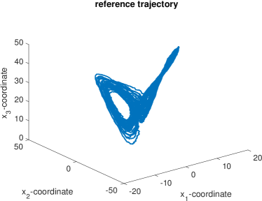
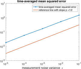
Figure 1: Reference trajectory (left panel) and time-averaged mean squared error as a function of the measurement error variance $\varepsilon$ (right panel).

   

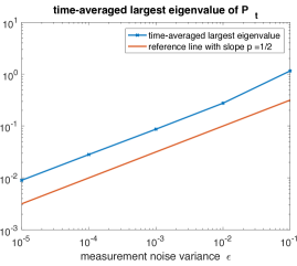
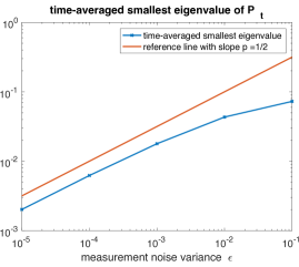
Figure 2: Time-averaged largest (left panel) and smallest (right panel) eigenvalues of $P_{t}$ as a function of the measurement error variance $\varepsilon$

We consider the stochastically perturbed Lorenz-63 system [Lor63, LSZ15], which leads to $N_{x}=3$, $D=C=I_{3}$, and drift term given by

$$f(x)=\left(\begin{array}[]{l}10(x_{2}-x_{1})\\ (28-x_{3})x_{1}-x_{2}\\ x_{1}x_{2}-\frac{8}{3}x_{3}\end{array}\right),$$ (128)

where $x=(x_{1},x_{2},x_{3})^{\rm T}$. Solutions of the Lorenz-63 system diverge exponentially fast and filtering is required in order to track a reference solution. Although (128) is only locally Lipschitz continuous, the results from this paper are likely to be applicable to the Lorenz-63 system due to the existence of a Lyapunov function.

We apply the EnKBF with ensemble size $M=4$ for values of the measurement error variances $\varepsilon\in\{10^{-1},\ldots,10^{-4},10^{-5}\}$. The stochastic evolution equations of the EnKBF are solved by the following modified Euler-Maruyama scheme

$$X^{i}_{n+1}=X_{n}^{i}+\Delta tf(X_{n}^{i})+\Delta t(P^{M}_{n})^{-1}(X_{n}^{i}-\bar{x}^{M}_{n})-\frac{1}{2}P_{n}^{M}\left(P_{n}^{M}+\frac{\varepsilon}{\Delta t}I_{3}\right)^{-1}\left(X_{n}^{i}+\bar{x}_{n}^{i}-2\frac{\Delta Y_{n}}{\Delta t}\right)$$ (129)

with step-size $\Delta t=0.00005$ over a total of $10^{7}$ time-steps. Note that

$$\left(P_{n}^{M}+\frac{\varepsilon}{\Delta t}I_{3}\right)^{-1}\approx\frac{\Delta t}{\epsilon}I_{3}$$ (130)

for $\Delta t$ sufficiently small and the modification is introduced for numerical stability reasons. See [AKIR14] for more details.

The results can be found in Figures 1 and 2. The numerical results are in agreement with our theoretical findings, which predicted an ${\cal O}(\varepsilon^{1/2})$ behavior of these quantities. While this scaling holds for the time-averaged mean squared error and the time-averaged largest eigenvalue of $P_{t}^{M}$ for the whole range of considered values of $\varepsilon$, the time-averaged smallest eigenvalue truncates slightly off for the larger values of $\varepsilon$. We can also see that there is a gap between the smallest and largest eigenvalues of $P_{t}^{M}$ on average.

We repeated the experiment for ensemble sizes of $M=2$ and $M=3$, in which case $P_{t}^{M}$ is singular. We still find that the time-averaged mean squared error is roughly of ${\cal O}(\varepsilon^{1/2})$. See Figure 3. The results are in line with those obtained in [GTH13] for hyperbolic dynamical systems. We will further investigate the theoretical properties of the EnKBF under singular $P_{t}^{M}$ in a separate paper.

   

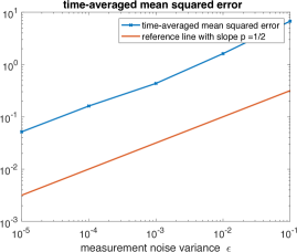
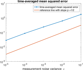
Figure 3: Time-averaged mean squared error as a function of the measurement error variance $\varepsilon$ for ensemble sizes $M=2$ (left panel) and $M=3$ (right panel).

7 Conclusions

In this paper, we have taken first steps towards an understanding of the long-time behavior of the ensemble Kalman-Bucy filter and have derived limiting mean-field equations. Natural extensions include partially observed processes and configurations which lead to singular empirical covariance matrices $P_{t}^{M}$. We also plan to extend our analysis to other ensemble filter algorithms, such as the stochastically perturbed ensemble Kalman-Bucy filter and the ensemble transform particle filter. See, for example, [RC15] for more details.

Appendix: Supplement to the proof of Theorem 5.4

The purpose of this Appendix is to provide two Lemmata on the control of $\|P_{t}^{M}-{\cal P}_{t}\|_{F}$ and on the existence of exponential moments of $\int_{0}^{t}\frac{1}{M}\sum_{i=1}^{M}\|\hat{X}_{s}^{i}\|^{2}{\rm d}s$ used in the proof of Theorem 5.4.

Lemma 7.1.

$$\|P_{t}^{M}-\mathcal{P}_{t}\|_{F}\leq 2\Sigma(t)\left(\frac{1}{M-1}\sum_{i}\|X_{t}^{i}-\hat{X}_{t}^{i}\|^{2}\right)^{\frac{1}{2}}+R_{M}(t)$$ (131)

with $\lim_{M\to\infty}R_{M}(t)=0$ a.s. and in $L^{1}(\mathbb{P})$. Here

$$\Sigma(t):=\left(\frac{1}{M-1}\sum_{i}\|X_{t}^{i}-\bar{x}_{t}^{M}\|^{2}\right)^{\frac{1}{2}}+\left(\frac{1}{M-1}\sum_{i}\|\hat{X}_{t}^{i}-\bar{x}_{t}\|^{2}\right)^{\frac{1}{2}}\,.$$ (132)

Similarly,

$$\|Q_{t}^{M}-\mathcal{Q}_{t}\|_{F}\leq 2(1+\|h\|_{\rm Lip})\Sigma(t)\left(\frac{1}{M-1}\sum_{i}\|X_{t}^{i}-\hat{X}_{t}^{i}\|^{2}\right)^{\frac{1}{2}}+S_{M}(t)$$ (133)

with $\lim_{M\to\infty}S_{M}(t)=0$ a.s. and in $L^{1}(\mathbb{P})$.

Remark 7.2.

Note that the factor $\Sigma(t)$ is locally bounded in $t$ due to Lemma 5.2 and an appropriate generalization of Lemma 2.4.

Proof.

(of Lemma 7.1) First note that we can decompose

$$P_{t}^{M}-\mathcal{P}_{t} =\frac{1}{M-1}\sum_{i=1}^{M}\left(X_{t}^{i}-\bar{x}_{t}^{M}\right)\left(X_{t}^{i}-\bar{x}_{t}^{M}\right)^{\rm T}-\mathbb{E}\left[\left(\hat{X}_{t}-\bar{x}_{t}\right)\left(\hat{X}_{t}-\bar{x}_{t}\right)^{\rm T}\right]$$ (134)

$$=\frac{1}{M-1}\sum_{i=1}^{M}\left(X_{t}^{i}-\bar{x}_{t}^{M}-\left(\hat{X}_{t}^{i}-\bar{x}_{t}\right)\right)\left(X_{t}^{i}-\bar{x}_{t}^{M}\right)^{\rm T}$$

$$\qquad+\frac{1}{M-1}\sum_{i=1}^{M}\left(\hat{X}_{t}^{i}-\bar{x}_{t}\right)\left(X_{t}^{i}-\bar{x}_{t}^{M}-\left(\hat{X}_{t}^{i}-\bar{x}_{t}\right)\right)^{\rm T}$$

$$\qquad+\frac{1}{M-1}\sum_{i=1}^{M}\left(\hat{X}_{t}^{i}-\bar{x}_{t}\right)\left(\hat{X}_{t}^{i}-\bar{x}_{t}\right)^{T}-\mathbb{E}\left[\left(\hat{X}_{t}-\bar{x}_{t}\right)\left(\hat{X}_{t}-\bar{x}_{t}\right)^{\rm T}\right]$$

$$=I+II+III\,.$$

In particular, $\|P_{t}^{M}-\mathcal{P}_{t}\|_{\rm F}\leq\|I\|_{\rm F}+\|II\|_{\rm F}+\|III\|_{\rm F}$. Term $I$ can be estimated from above by

$$\|I\|_{\rm F} \leq\left(\frac{1}{M-1}\sum_{i=1}^{M}\|X_{t}^{i}-\bar{x}_{t}^{M}-\left(\hat{X}_{t}^{i}-\bar{x}_{t}\right)\|^{2}\right)^{1/2}\left(\frac{1}{M-1}\sum_{i=1}^{M}\|X_{t}^{i}-\bar{x}_{t}^{M}\|^{2}\right)^{1/2}$$ (135)

$$\leq\left(\left(\frac{1}{M-1}\sum_{i=1}^{M}\|X_{t}^{i}-\hat{X}_{t}^{i}\|^{2}\right)^{1/2}+\sqrt{\frac{M}{M-1}}\|x_{t}^{M}-\bar{x}_{t}\|\right)\left(\frac{1}{M-1}\sum_{i=1}^{M}\|X_{t}^{i}-\bar{x}_{t}^{M}\|^{2}\right)^{1/2}$$

$$\leq\left(2\left(\frac{1}{M-1}\sum_{i=1}^{M}\|X_{t}^{i}-\hat{X}_{t}^{i}\|^{2}\right)^{1/2}+\sqrt{\frac{M}{M-1}}\left\|\frac{1}{M}\sum_{i=1}^{M}\hat{X}_{t}^{i}-\mathbb{E}\left[\hat{X}_{t}^{i}\right]\right\|\right)$$

$$\qquad\qquad\left(\frac{1}{M-1}\sum_{i=1}^{M}\|X_{t}^{i}-\bar{x}_{t}^{M}\|^{2}\right)^{1/2}\,.$$

Similarly,

$$\|II\|_{\rm F} \leq\left(2\left(\frac{1}{M-1}\sum_{i=1}^{M}\|X_{t}^{i}-\hat{X}_{t}^{i}\|^{2}\right)^{1/2}+\sqrt{\frac{M}{M-1}}\left\|\frac{1}{M}\sum_{i=1}^{M}\hat{X}_{t}^{i}-\mathbb{E}\left[\hat{X}_{t}^{i}\right]\right\|\right)$$ (136)

$$\qquad\qquad\left(\frac{1}{M-1}\sum_{i=1}^{M}\|\hat{X}_{t}^{i}-\bar{x}_{t}\|^{2}\right)^{1/2}\,.$$

Finally,

$$\|III\|_{\rm F} =\left\|\frac{1}{M}\sum_{i=1}^{M}\left(\hat{X}_{t}^{i}(\hat{X}_{t}^{i})^{\rm T}-\mathbb{E}\left[\hat{X}_{t}^{i}(\hat{X}_{t}^{i})^{\rm T}\right]\right)+\frac{1}{M(M-1)}\left(\hat{X}_{t}^{i}-\bar{x}_{t}\right)\left(\hat{X}_{t}^{i}-\bar{x}_{t}\right)^{\rm T}\right\|_{\rm F}$$ (137)

$$\leq\left\|\frac{1}{M}\sum_{i=1}^{M}\left(\hat{X}_{t}^{i}(\hat{X}_{t}^{i})^{\rm T}-\mathbb{E}\left[\hat{X}_{t}^{i}(\hat{X}_{t}^{i})^{\rm T}\right]\right)\right\|_{\rm F}+\frac{1}{M}\left\|\frac{1}{M-1}\sum_{i=1}^{M}\left(\hat{X}_{t}^{i}-\bar{x}_{t}\right)\left(\hat{X}_{t}^{i}-\bar{x}_{t}\right)^{\rm T}\right\|_{\rm F}$$

Adding up all terms we arrive at the estimate

$$\|P_{t}^{M}-\mathcal{P}_{t}\|_{\rm F} \leq 2\Sigma(t)\left(\frac{1}{M-1}\sum_{i=1}^{M}\|X_{t}^{i}-\hat{X}_{t}^{i}\|^{2}\right)^{1/2}+R_{M}(t)$$ (138)

with the remainder

$$R_{M}(t) =\Sigma(t)\sqrt{\frac{M}{M-1}}\left\|\frac{1}{M}\sum_{i=1}^{M}\hat{X}_{t}^{i}-\mathbb{E}\left[\hat{X}_{t}^{i}\right]\right\|+\|III\|_{\rm F}\,.$$ (139)

The strong law of large numbers now implies that $\lim_{M\to\infty}R_{M}(t)=0$ in a.s. and in $L^{1}(\mathbb{P})$. The proof of the second estimate is done similarly. ∎

Lemma 7.3.

Let $\hat{X}_{t}^{i}$, $1\leq i\leq M$, $M\geq 2$, be the solution of (11) with initial conditions iid ($\pi_{0}$) and suppose that $\pi_{0}$ has bounded support contained in a ball with radius $K$. Then for all $T>0$ there exist $\delta_{0}>0$ and $\kappa_{0}>0$ depending on $T$, but independent of $M$, such that

$$\mathbb{E}\left[e^{\delta_{0}\int_{0}^{t}\frac{1}{M}\sum_{i=1}^{M}\|\hat{X}_{s}^{i}\|^{2}{\rm d}s}\right]\leq e^{2\kappa_{0}\left(\frac{K^{2}}{M}+\left\|h\left(X^{\rm ref}_{0:T}\right)\right\|^{2}_{\infty}\right)}<+\infty\quad\forall\,t\leq T\,.$$ (140)

Here, the expectation is taken also w.r.t. the distribution of $\{Y_{s}\}$.

Proof.

First note that Itô’s formula and (11) imply that

$${\rm d}\left(\frac{1}{M}\sum_{i=1}^{M}\|\hat{X}_{t}^{i}\|^{2}\right) =\frac{2}{M}\sum_{i=1}^{M}\langle f\left(\hat{X}_{t}^{i}\right),\hat{X}_{t}^{i}\rangle{\rm d}t+\frac{2}{M}\sum_{i=1}^{M}\langle D\mathcal{P}_{t}^{-1}\left(\hat{X}_{t}^{i}-\bar{x}_{t},\right),\hat{X}_{t}^{i}\rangle{\rm d}t$$ (141)

$$\qquad-\frac{1}{M}\sum_{i=1}^{M}\langle\mathcal{Q}_{t}R^{-1}h\left(\hat{X}_{t}^{i}\right),\hat{X}_{t}^{i}\rangle{\rm d}t-\frac{1}{M}\sum_{i=1}^{M}\langle\mathcal{Q}_{t}R^{-1}\bar{h}_{t},\hat{X}_{t}^{i}\rangle{\rm d}t$$

$$\qquad+\frac{2}{M}\sum_{i=1}^{M}\langle\hat{X}_{t}^{i},\mathcal{Q}_{t}R^{-1}{\rm d}Y_{t}\rangle+\frac{1}{M}\mbox{tr}\left(\mathcal{Q}_{t}R^{-1}\mathcal{Q}_{t}\right){\rm d}t\,.$$

Using Lipschitz continuity of $f$ and $h$ and the previous two Lemmata 5.2 and 5.3, the right hand side can be estimated from above for $t\leq T$ by

$$C(T)\left(1+\frac{1}{M}\sum_{i=1}^{M}\|\hat{X}_{t}^{i}\|^{2}\right)+\frac{2}{M}\sum_{i=1}^{M}\langle\hat{X}_{t}^{i},\mathcal{Q}_{t}R^{-1}{\rm d}Y_{t}\rangle$$ (142)

for some uniform constant $C(T)$. Since ${\rm d}Y_{t}=h\left(X^{\rm ref}_{t}\right){\rm d}t+R^{-1/2}{\rm d}B_{t}$ we can further estimate from above for $t\leq T$

$$C(T)\left(1+\left\|h\left(X^{\rm ref}_{t}\right)\right\|^{2}+\frac{1}{M}\sum_{i=1}^{M}\|\hat{X}_{t}^{i}\|^{2}\right)+\frac{2}{M}\sum_{i=1}^{M}\langle\hat{X}_{t}^{i},\mathcal{Q}_{t}R^{-1/2}{\rm d}B_{t}\rangle$$ (143)

for some possibly different constant $C(T)$. Itô’s product rule now implies for $\alpha:=1+C(T)$ and $t\leq T$

$${\rm d}\left(e^{-\alpha t}\frac{1}{M}\sum_{i=1}^{M}\|\hat{X}_{t}^{i}\|^{2}\right) \leq e^{-\alpha t}C(T)\left(1+\left\|h\left(X^{\rm ref}_{t}\right)\right\|^{2}\right)\,{\rm d}t-e^{-\alpha t}\left(\frac{1}{M}\sum_{i=1}^{M}\|\hat{X}_{t}^{i}\|^{2}\right){\rm d}t$$ (144)

$$\qquad+e^{-\alpha t}\frac{2}{M}\sum_{i=1}^{M}\langle\hat{X}_{t}^{i},\mathcal{Q}_{t}R^{-1/2}{\rm d}B_{t}\rangle\,,$$

which implies that

$$\int_{0}^{t}e^{-\alpha s}\frac{1}{M}\sum_{i=1}^{M}\|\hat{X}_{s}^{i}\|^{2}{\rm d}s \leq\frac{1}{M}\sum_{i=1}^{M}\|\hat{X}_{0}^{i}\|^{2}+C(T)\left(1+\left\|h\left(X^{\rm ref}_{0:T}\right)\right\|^{2}_{\infty}\right)$$ (145)

$$\qquad+\int_{0}^{t}e^{-\alpha s}\frac{2}{M}\sum_{i=1}^{M}\langle\hat{X}_{s}^{i},\mathcal{Q}_{t}R^{-1/2}{\rm d}B_{s}\rangle\,.$$

To simplify notations in the following let

$$M_{t}:=\int_{0}^{t}e^{-\alpha s}\frac{2}{M}\sum_{i=1}^{M}\langle\hat{X}_{s}^{i},\mathcal{Q}_{t}R^{-1/2}{\rm d}B_{s}\rangle$$ (146)

and observe that the quadratic variation $\langle M\rangle_{t}$ can be estimated from above by

$$\langle M\rangle_{t} =\frac{4}{M^{2}}\sum_{i=1}^{M}\int_{0}^{t}e^{-2\alpha s}\|R^{-1/2}\mathcal{Q}^{T}_{s}\hat{X}_{s}^{i}\|^{2}{\rm d}s$$ (147)

$$\leq\frac{4\|R^{-1/2}\|^{2}_{\rm F}\|h\|_{\rm Lip}^{2}C(T)^{2}}{M}\int_{0}^{t}e^{-\alpha s}\frac{1}{M}\sum_{i=1}^{M}\|\hat{X}_{s}^{i}\|^{2}{\rm d}s\,,$$

using

$$\|\mathcal{Q}_{s}\|^{2}_{\rm F}\leq\|h\|_{\rm Lip}^{2}\mathbb{E}\left[\|\hat{X}_{s}-\bar{x}_{s}\|^{2}\right]\leq\|h\|_{\rm Lip}^{2}C(T)^{2}$$ (148)

and Lemma 5.2. The assumption on the initial condition now implies for $\delta>0$

$$\mathbb{E}\left[e^{\delta\int_{0}^{t}e^{-\alpha s}\frac{1}{M}\sum_{i=1}^{M}\|\hat{X}_{s}^{i}\|^{2}\,ds}\right] \leq e^{\delta\left(\frac{K^{2}}{M}+C(T)\left(1+\left\|h\left(X^{\rm ref}_{0:T}\right)\right\|^{2}_{\infty}\right)\right)}\mathbb{E}\left[e^{\delta M_{t}}\right]$$ (149)

$$\leq e^{\delta\left(\frac{K^{2}}{M}+C(T)\left(1+\left\|h\left(X^{\rm ref}_{0:T}\right)\right\|^{2}_{\infty}\right)\right)}\mathbb{E}\left[e^{2\delta^{2}\langle M\rangle_{t}}\right]^{1/2}$$

$$\leq e^{\delta\left(\frac{K^{2}}{M}+C(T)\left(1+\left\|h\left(X^{\rm ref}_{0:T}\right)\right\|^{2}_{\infty}\right)\right)}$$

$$\qquad\mathbb{E}\left[e^{2\delta\frac{4\|R^{-1/2}\|^{2}_{\rm F}\|h\|_{\rm Lip}^{2}C(T)^{2}}{M}\delta\int_{0}^{t}e^{-\alpha s}\frac{1}{M}\sum_{i=1}^{M}\|\hat{X}_{s}^{i}\|^{2}{\rm d}s}\right]^{1/2}\,,$$

thereby using the inequality

$$\mathbb{E}\left[e^{\delta M_{t}}\right] =\mathbb{E}\left[e^{\frac{1}{2}\left(2\delta M_{t}-2\delta^{2}\langle M\rangle_{t}\right)}e^{\frac{1}{2}\left(2\delta^{2}\langle M\rangle_{t}\right)}\right]\leq\mathbb{E}\left[e^{2\delta M_{t}-2\delta^{2}\langle M\rangle_{t}}\right]^{1/2}\mathbb{E}\left[e^{2\delta^{2}\langle M\rangle_{t}}\right]^{1/2}$$ (150)

$$=\mathbb{E}\left[e^{2\delta^{2}\langle M\rangle_{t}}\right]^{1/2}\,.$$

Hence for $\delta_{0}>0$ with

$$\delta_{0}\frac{8\|R^{-1/2}\|_{\rm F}^{2}\|h\|_{\rm Lip}^{2}C(T)^{2}}{M}<1$$ (151)

it follows that

$$\mathbb{E}\left[e^{\delta_{0}\int_{0}^{t}e^{-\alpha s}\frac{1}{M}\sum_{i=1}^{M}\|\hat{X}_{s}^{i}\|^{2}{\rm d}s}\right] \leq e^{2\delta_{0}\left(\frac{K^{2}}{M}+C(T)\left(1+\left\|h\left(X^{\rm ref}_{0:T}\right)\right\|^{2}_{\infty}\right)\right)}<e^{2\kappa_{0}\left(\frac{K^{2}}{M}+\left\|h\left(X^{\rm ref}_{0:T}\right)\right\|^{2}_{\infty}\right)}<+\infty\$$ (152)

for a suitable $\kappa_{0}>0$. ∎

References

• [AKIR14] J. Amezcua, E. Kalnay, K. Ide, and S. Reich. Ensemble transform Kalman-Bucy filters. Q.J.R. Meteor. Soc., 140:995–1004, 2014.
• [AMGC02] M.S. Arulampalam, S. Maskell, N. Gordon, and T. Clapp. A tutorial on particle filters for online nonlinear/non-Gaussian Bayesian tracking. IEEE Trans. Sign. Process., 50:174–188, 2002.
• [BC08] A. Bain and D. Crisan. Fundamentals of stochastic filtering, volume 60 of Stochastic modelling and applied probability. Springer-Verlag, New-York, 2008.
• [BR10] K. Bergemann and S. Reich. A localization technique for ensemble Kalman filters. Q. J. R. Meteorological Soc., 136:701–707, 2010.
• [BR12] K. Bergemann and S. Reich. An ensemble Kalman-Bucy filter for continuous data assimilation. Meteorolog. Zeitschrift, 21:213–219, 2012.
• [BY82] M. Barlow and M. Yor. Semi-martingale inequalities via the Garcia-Rodemich-Rumsey lemma, and applications to local times. Journal of Functional Analysis, 49:198–229, 1982.
• [DdFe01] A. Doucet, N. de Freitas, and N. Gordon (eds.). Sequential Monte Carlo methods in practice. Springer-Verlag, Berlin Heidelberg New York, 2001.
• [DE99] L. Dieci and T. Eirola. On smooth decompositions of matrices. SIAM J. Matrix Anal., 20:800–819, 1999.
• [DMKT16] P. Del Moral, A. Kurtzmann, and J. Tugaut. On the stability and the uniform propagation of chaos of extended ensemble Kalman-Bucy filters. Technical Report arXiv:1606.08256v1, INRIA Bordeaux Research Center, 2016.
• [Eve06] G. Evensen. Data assimilation. The ensemble Kalman filter. Springer-Verlag, New York, 2006.
• [GMT11] F. Le Gland, V. Monbet, and V.D. Tran. Large sample asymptotics for the ensemble Kalman filter. In The Oxford Handbook of Nonlinear Filtering, pages 598–631, Oxford, 2011. Oxford University Press.
• [GTH13] C. González-Tokman and B.R. Hunt. Ensemble data assimilation for hyperbolic systems. Physica D, 243:128–142, 2013.
• [Jaz70] A.H. Jazwinski. Stochastic processes and filtering theory. Academic Press, New York, 1970.
• [KLS14] D. T. Kelly, K. J. H. Law, and A. Stuart. Well-posedness and accuracy of the ensemble Kalman filter in discrete and continuous time. Nonlinearity, 27:2579–2604, 2014.
• [KM15] E. Kwiatowski and J. Mandel. Convergence of the square root ensemble Kalman filter in the large ensemble limit. SIAM/ASA J. Uncertainty Quantification, 3:1–17, 2015.
• [KMT15] D. Kelly, A.J. Majda, and X.T. Tong. Concrete ensemble Kalman filters with rigorous catastrophic filter divergence. Proc. Natl. Acad. Sci. USA, 112:10589–10594, 2015.
• [KS72] Kwakernaak and Sivan. Linear Optimal Control Systems. Wiley Interscience, New York, 1972.
• [Lor63] E.N. Lorenz. Deterministic non-periodic flows. J. Atmos. Sci., 20:130–141, 1963.
• [LSZ15] K. Law, A. Stuart, and K. Zygalakis. Data Assimilation: A Mathematical Introduction. Springer-Verlag, New York, 2015.
• [MH12] A. Majda and J. Harlim. Filtering Complex Turbulent Systems. Cambridge University Press, Cambridge, 2012.
• [Mor13] P. Del Moral. Mean field simulation for Monte Carlo integration. Chapman & Hall, London, 2013.
• [Øks00] B. Øksendal. Stochastic Differential Equations. Springer-Verlag, Berlin-Heidelberg, 5th edition, 2000.
• [OP96] D. Ocone and E. Pardoux. Asymptotic stability of the optimal filter with respect to its initial condition. SIAM J. Control and Optimization, 34:226–243, 1996.
• [RC15] S. Reich and C.J. Cotter. Probabilistic Forecasting and Bayesian Data Assimilation. Cambridge University Press, Cambridge, 2015.
• [Rei11] S. Reich. A dynamical systems framework for intermittent data assimilation. BIT Numer Math, 51:235–249, 2011.
• [Rel69] F. Rellich. Perturbation Theory for Linear Operators. Gordon and Breach, New York, 1969.
• [TMK16] X.T. Tong, A.J. Majda, and D. Kelly. Nonlinear stability and ergodicity of ensemble based Kalman filters. Nonlinearity, 29(2):657, 2016.
• [Ton17] X.T. Tong. Performance analysis of local ensemble Kalman filter. Technical Report arXiv:1705.10598, National University of Singapore, 2017.