Mixing Times and Structural Inference for Bernoulli Autoregressive Processes
Abstract
We introduce a novel multivariate random process producing Bernoulli outputs per dimension, that can possibly formalize binary interactions in various graphical structures and can be used to model opinion dynamics, epidemics, financial and biological time series data, etc. We call this a Bernoulli Autoregressive Process (BAR). A BAR process models a discrete-time vector random sequence of scalar Bernoulli processes with autoregressive dynamics and corresponds to a particular Markov Chain. The benefit from the autoregressive dynamics is the description of a transition matrix by at most effective parameters for some or by two sparse matrices of dimensions and , respectively, parameterizing the transitions. Additionally, we show that the BAR process mixes rapidly, by proving that the mixing time is . The hidden constant in the previous mixing time bound depends explicitly on the values of the chain parameters and implicitly on the maximum allowed in-degree of a node in the corresponding graph. For a network with nodes, where each node has in-degree at most and corresponds to a scalar Bernoulli process generated by a BAR, we provide a greedy algorithm that can efficiently learn the structure of the underlying directed graph with a sample complexity proportional to the mixing time of the BAR process. The sample complexity of the proposed algorithm is nearly order-optimal as it is only a factor away from an information-theoretic lower bound. We present simulation results illustrating the performance of our algorithm in various setups, including a model for a biological signaling network.
Keywords: Autoregressive, Glauber dynamics, mixing time, networked process, Markov chain, structural learning.
1 Introduction
Dynamical systems which evolve over networks are ubiquitous: examples include epidemic and opinion dynamics over social networks, gene regulatory networks, and stock/option price dynamics in financial markets [5, 7, 8, 27, 30, 34]. We model the interactions between the nodes in a network of this type using directed edges, where an edge from node to node indicates that the state of node at one time instant affects the state of node at the next time instant. Our goal is to infer such a directed graph from time series data. To this end, the mixing properties of the corresponding dynamical system become critical in determining sufficient sample complexities for consistent structure estimators.
Prior to performing inference on dynamical system data, one has to select a model class for the underlying dynamics. Modeling the dynamics of a multivariate process is a core subproblem of system identification [16, 24]. The work in this paper can be thought as laying the groundwork for performing discrete system identification in the class of Bernoulli Autoregressive Processes (BAR) that are defined later and determining their mixing properties. Traditionally, the identification literature deals with the problem of estimating the unknown parameters of a system model directly; however, in the machine learning literature, the problem is broken down into two steps: first, structure learning and second, parameter estimation. Structure learning refers to the problem of estimating whether each parameter is positive, negative, or zero. Here, we focus only on the structure learning problem; parameter estimation is typically a simpler problem once the structure is known. When the state variables take continuous values, structure learning can be related to Lasso-type sparse inference ideas (see [7]) or more traditional system-theoretic filtering ideas [27]. However, to the best of our knowledge, these ideas do not directly apply to models where the state variables take on discrete values, as in our BAR model.
A related approach to discrete system identification is what is known as causal network inference. Historically, this problem is linked to the notion of Granger causality [17]. The goal in [17] was the description of a hypothesis test to determine whether a time series can be used to improve the predictability of another time series. The problem was initially formalized to tackle the case of linear dynamics. Granger causality has been more recently incorporated and extended in information theory through the notion of directed information. Following the pioneering work of Marko [25], the notion of directed information was first introduced by Massey [26], as a measure of the information flow from one random sequence to another in a synchronized fashion. Later on, Kramer introduced the notion of causal conditioning in probability distributions. Connecting the latter with directed information, Kramer was able to analyze the capacity of systems with feedback [21, 22]. Whenever there is feedback between the input and the output of a system, the directivity of information flow becomes significant. Very recently, directed information has been used to perform causal network inference of networked dynamical processes [30]. The approach is very generally applicable, but here we are interested in developing algorithms, which have good sample and computational complexities when applied to a specific model class.
If the underlying model does not have dynamics, i.e., the state of the system at one time instant does not affect the state of the system at the next time instant, then the discrete system identification problem reduces to the problem of learning graphical models from independent samples. Graphical models constitute a powerful statistical tool used to represent joint probability distributions, with the underlying graph dictating the way that these distributions factorize. The associated graphs are most often undirected giving rise to Markov random fields, while the data are often considered to be i.i.d. [3, 4, 9, 35]. The associated graphs can also be directed and acyclic giving rise to Bayesian networks, which possess a different set of properties from Markov random fields [35]. The graphical structure affects the computational complexity associated with different statistical inference tasks such as computing marginals, posterior probabilities, maximum a posteriori estimates and sampling from the corresponding distributions. The absence of an edge in such graphs represents conditional independence between two nodes or random variables given the rest of the network. Our problem can be thought as that of learning a directed network in which the output at one time instant becomes the input to the next time instant.
1.1 Main Results
In this paper, we introduce a novel multivariate dynamical process producing Bernoulli outputs at each node in a network, that can possibly formalize binary interactions in various graphical structures. We call this a Bernoulli Autoregressive Process. A BAR models a Bernoulli vector process with linear dynamics imposed on the parameters of the associated Bernoulli random variables and corresponds to a special form of Markov chain with a directed underlying graphical structure. Assuming nodes in the network, we first prove that any BAR process mixes very rapidly by showing that for any . Motivated by the operation of local Markov chains including the Glauber dynamics, we also introduce in Section 9 two BAR random walks on the hypercube and under a column-substochasticity assumption on the dynamics, we prove that in this case. If each node has in-degree at most and corresponds to a scalar Bernoulli process generated by a BAR, we provide a greedy algorithm that can learn the structure of the underlying directed graph with computational complexity of order for a sufficient number of samples proportional to the mixing time of the BAR process. The aforementioned structure estimator is shown to be nearly order-optimal requiring a sample complexity that is only a multiple of away from a lower information-theoretic bound.
1.2 Other Related Work
In their influential paper [13], Chow and Liu showed that learning a tree-structured Markov random field can be achieved with time complexity of order , when the graph has nodes. Very recently, Bresler provided a method to learn the structure of Ising models with nodes of degree at most in time , where is a constant depending doubly-exponentially on and the range of interaction strengths in the Ising model [9]. Exponential dependence on is unavoidable in binary graphical models as it has been shown in [33]. [13] and [9] perform structure learning of graphical models based on i.i.d. samples. In the more relevant work [10], the problem of learning undirected graphical models based on data generated by the Glauber dynamics is examined. The Glauber dynamics is a special form of a reversible Markov chain and it is often used in the context of Markov Chain Monte Carlo algorithms to sample from a distribution of interest. The key observation in [10] is that the problem of learning graphs by observing the Glauber dynamics is computationally tractable. Our work differs from the assumptions in [10] in that the corresponding graph for a BAR process is directed and at any time instant the individual states of ultimately all nodes can be updated. The problem of learning the graphical structure of a general Markov time series is examined in [12]. The proposed approach is relevant to the notion of causal entropy, which is very similar in nature to directed information. The corresponding sample complexity depends logarithmically on the dimension of the process and linearly on the mixing time, while the computational complexity is . The problem of learning from epidemic cascades has been considered in [29, 31] and [28], while a number of papers have studied the problem of learning functions or concepts by observing Markov chain sample paths [2, 6, 15]. Finally, a relevant model to the BAR is the so-called ALARM introduced in [1]. ALARM differs from the BAR in the use of the logistic function in defining the transition probabilities, which allows linear (positive and negative) coefficients in the autoregressive dynamics. Nevertheless, the interpretability of the model parameters is not as straighforward as in the BAR model. In addition, we can easily devise examples of BAR chains in which the transitions cannot be exactly described by the ALARM model. Moreover, to the best of our knowledge, no mixing time analysis of the ALARM model exists, while the proposed algorithm for recovering the structure of the network is based on a straightforward application of regularization, i.e., Lasso and group-Lasso. It is well-known that convex optimization approaches like Lasso and group-Lasso for model selection have very poor performance, when the observed data have temporal dependencies as in our case [36, 37]. Further analysis details would be of interest, e.g., recovery guarantees, sample complexity and mixing properties of the ALARM model.
1.3 Organization
Section 2 informally presents the contributions of this paper. The BAR model is introduced in Section 3. Section 4 formulates the BAR structure learning problem, while the proposed BAR structure observer is formalized. The main results in this paper and their proofs are presented in Sections 5, 6 and 7. Section 8 provides a lower information-theoretic bound on the necessary sample complexity for any BAR structure estimator, verifying that the proposed algorithm is nearly order-optimal. Random walk variants of the BAR model along with their mixing properties are provided in Section 9, completing the palette of BAR processes. Finally, numerical examples are provided in Section 10 and the paper is concluded in Section 11.
2 Main Contributions: A Conceptual Overview
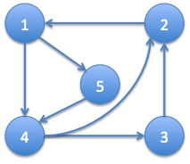
In this section, we informally discuss and provide intuitive interpretations of our results. The graphical structure of a BAR process can be visualized as in Fig. 1(a), where for simplicity we assume that . Each node corresponds to a scalar Bernoulli random process. The arrows represent causal relationships between the nodes. The problems that we consider are to evaluate the mixing time of any BAR process and to identify the parental sets of all nodes in the graph, i.e., the set of nodes whose states at one time instant affect the state of any given node at the next time instant. We assume that the in-degree of each node is at most . Our main results are the following:
Theorem 1
(BAR, Mixing Time-informal) Consider a BAR process corresponding to an arbitrary graph with nodes, where each node has in-degree at most . This process corresponds to a special kind of Markov chains with a directed graphical structure. For any , the BAR process mixes rapidly with . The hidden terms in notation depend explicitly on and the parameter values defining the BAR model and implicitly on . Moreover, the BAR random walks corresponding to the same network also mix rapidly with , when the dynamics satisfy a column-substochasticity assumption. The hidden terms in notation depend explicitly on , the parameter values defining the BAR random walk, the probability of being lazy and implicitly on
Theorem 2
(BAR, Algorithm Performance-informal) Consider the BAR model on an arbitrary graph with nodes, where each node has in-degree at most . Given samples from the model for some , it is possible to learn the underlying graph using computations. Here, is a function of and the parameter values defining the BAR model. Moreover, since , corresponds to having absorbed the mixing bound constant.
The parental set or parental neighborhood of each node in the graph is separately estimated. To obtain the necessary accuracy in the required statistics for the proposed algorithm, the order of the sample complexity can be proved to be . To decide the edge set of the graph, i.e., the existence of arrows and their orientations, the algorithm has to initially examine all possible pairs of nodes separately, the number of which is . Given the required computations per sample, it turns out that the complexity of the algorithm is due to a constant upper bound imposed on by the definition of the BAR model, as we will see shortly. Further, the proposed algorithm for learning the structure of a BAR process can determine if a node affects another node positively or negatively.
3 Bernoulli Autoregressive Processes
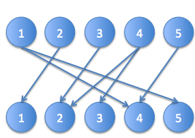
We consider a directed graph with nodes (Fig. 1(a)). We can associate with this graph a bipartite graph, where the two parts have the same vertex set (Fig. 1(b)). For each node in the upper part we have directed links to the lower part only to those nodes that points to or causally affects. Although Fig. 1(b) is illuminating, we will focus on Fig. 1(a) from now on and we will consider a directed graph , the topology of which we would like to infer based on a particular form of Bernoulli time series data to be specified shortly.
The state of each node in is assumed to be a Bernoulli random variable (r.v.) . The state vector is considered to be observable. We will denote a particular realization of by . Assuming that the state vector of at time instant is , the BAR updates the state vector as follows:
| (1) |
with a rowwise interpretation of . Additionally, is the matrix with the interpretation that are the corresponding diagonal elements (or blocks) and . Each corresponds to a vector and has the form
| (5) |
where we denote the parental neighborhood of node by . Here, stands for the unsigned support of a vector or a matrix. For the choice of either or is irrelevant; hence, we will assume from now on the convention in this case. Moreover, we consider the partition , where . The set of parents, which positively influence node , is denoted by and the set of parents, which negatively influence node , is denoted by . The simplest but also the most natural case assumes that , i.e., for all , resulting to
| (6) |
Here, is the matrix
| (7) |
Remark: can be always defined and will always be a reference matrix in our subsequent analysis, even in the case that it does not directly appear to the BAR model, as for example in (1).
In addition, is distributed according to and we write . are assumed to be i.i.d. vectors drawn from the product distribution with for any with , where denotes independence. As before, denotes a particular realization of . Furthermore, we assume that each has support size such that and for some . Additionally, is considered to be diagonal with and . To ensure that the parameters of the Bernoulli random variables in (1) lie in the interval [0,1], we assume that
| (8) |
These constraints show that is a square substochastic matrix and is a doubly substochastic matrix111 is diagonal.. Moreover, the imposed constraints on the values of the parameters and (8) imply that is upper bounded by , where is the integer solution of the following program:
| (9) |
The aforementioned rowwise interpretation of the in (1) has the meaning that given the argument , is independently drawn from . The term ensures persistence of excitation in the model. In this sense, it is sufficient to assume that is diagonal. Nevertheless, extensions to more general ’s are possible. Note that a consequence of the assumption that all the ’s are strictly positive is the prevention of the event that the model generates all-zeros or all-ones state vectors after a visit to a state that is all-zeros on and all-ones on or all-ones on and all-zeros on , respectively, at a particular time instant. The random sequence is referred to as the Bernoulli Autoregressive Process.
We now let . Then, with if , where is the directed link from node to node . We also let with , where ‘’ is used twice for notational convenience. Thus, for the graph , we define the set of valid parameter vectors as
4 BAR Learning
Let be the set of all directed graphs with nodes, each node having at most parents. For any graph in , we associate a sign or with each edge from to to indicate whether belongs to or as in (5). For some and a pair of parameter vectors , we assume that we initialize the system at , where is the stationary measure of the BAR process222We prove later on that every BAR process has a unique invariant measure.. We observe the sequence of correlated state vectors denoted by , where each is generated by (1). A BAR structure observer is a mapping:
The output
is the observer’s best estimate of the unsigned support of denoted by and of , where for all . To evaluate the performance of the BAR structure observer, we use the zero-one loss
Here, denotes the indicator of the event . The associated risk for some pair corresponding to is given by . For robustness, we focus on finding observers such that the worst case risk
tends to zero as with the least number of samples .
4.1 BAR Structure Observer
The proposed BAR structure observer operates in two stages:
-
•
Supergraph Selection: A supergraph of the actual graph is obtained.
-
•
Supergraph Trimming: The obtained supergraph from the previous stage is reduced to the actual graph by excluding nodes from the neighborhood of each node with no causal influence to this node.
The above two stages will be successful with high probability for a sufficient sample complexity.
4.1.1 Supergraph Selection
This stage will be based on the following measure of conditional influence:
| (10) |
Here, and refer to successive time instants. Also, the underlying measure in defining is the stationary, thus we have dropped the temporal indices in the involved random variables. The main reason motivating this metric is the desire of a good tradeoff between computational complexity and statistical efficiency in squeezing out structural information from the observed data. Similar measures have been used in prior work to define structure estimators, see for example [3, 4, 9, 10]. The difference in from prior measures is that the conditioning does not account for other nodes that possibly belong to the neighborhood of the th node. The key point here is that can be nonzero even when , since can be correlated with some or all . On the other hand, similar metrics in prior literature aim at defining by conditioning also with respect to . Clearly, if and is defined as
then if due to the Markov property and thus, for and , can only be zero. Our subsequent analysis shows that there is no significant loss in the BAR case from considering only conditioning with respect to a single node every time. Intuitively, the magnitude of quantifies what is the probability that causally affects either positively or negatively over the case of no influence. A more rigorous motivation for defining as the difference of the two conditional probabilities appearing in (10) is by considering reductions of relevant entropies. More specifically, pick an and let
and
characterizes the residual randomness in when and quantifies the corresponding residual randomness when . If is (causally) independent of , i.e., and is independent of all , then and . Thus, in this case. At the same time, and therefore, (causal) independence between and is totally characterized by . In the general case, consider the causal entropy and observe that
Thus, the differences and more or less control the magnitude of . Considering without loss of generality only the first difference, we have the following result:
Lemma 1
The difference critically depends on .
Proof
Appendix A.
In practice, we will work the empirical analogues
where and similarly for .
4.1.2 Supergraph Trimming
For the trimming stage, we assume that the upper bound is known, which is a very reasonable assumption333in the worst scenario, ., and has been used by the supergraph selection stage to deliver an overestimate with unknown edge labels (i.e., and have not been estimated yet). For a sufficiently large , the true graph is a subgraph of with high probability. Hence, our starting point is the assumption that the true graph is contained in . Let and assume without loss of generality that . Then,
| (11) |
If takes all binary vector values, then there is at least one binary vector such that
Therefore, corresponds to the maximum value that can take. If is unique, then we can safely conclude that and . Here, the subscript is reserved for “final estimates”. Furthermore, we can immediately extract and by placing in all corresponding to in and by placing in all corresponding to in . If is not unique, then we conclude that and there are such that . In this case, we collect all binary vectors corresponding to the maximum value of , namely , where . When but , there will be at least two binary vectors among the maximizers in which appears with the values and . This observation shows that we can estimate the final neighborhood by placing in all corresponding to either only the value in all maximizers or to only the value in all maximizers. Also, we can immediately extract and by placing in all corresponding to in all maximizers and by placing in all corresponding to in all maximizers.
In practice, we will empirically estimate by
where and similarly for . Empirical estimates cause the problem that almost surely will be maximized by a single binary vector , while there might be binary vectors corresponding to less variables than in the true neighborhood, yielding a value of close to the maximum. Here, is used on to denote that we refer to a maximizer of the empirical conditional probability measure. These problems can be resolved by observing the following:
-
•
As , for some . Here, stands for a ball with center and radius . Therefore, for sufficiently large , only the actual maximizers will yield almost maximum values for .
-
•
Every time a node does not participate in (11) with the appropriate polarity, is reduced by at least according to our assumptions. In other words, the possible distinct values that can take for all possible binary vectors differ by at least . Assuming that the maximum value of is , then for sufficiently large , we will have that for some . We can therefore pick , which is an estimate of , as the binary vector delivering the maximum empirical conditional probability and the rest of the maximizers as those binary vectors giving empirical conditional probability values within from .
Having described the above procedure, the final point to consider is the choice of an appropriate threshold such that the picked maximizers are the correct ones. If corresponds to , then the interval contains all the maximizers for sufficiently large . If corresponds to , then we must make sure that the interval contains no points. This leads to the conclusion that should be at most .
4.1.3 The Algorithm
The proposed BAR structure observer, which learns the support of and when the in-degrees of all nodes are upper bounded by , is given by Alg. 1.
Remarks:
-
1.
BARObs can be possibly stopped upon the termination of the supergraph selection stage if an overestimate of the actual graph is sufficient for the application at hand. Overestimates of and can be then obtained by placing in each all such that and in each all such that . The sufficient sample complexity such that only the supergraph selection stage is successful with probability at least is lower than the sufficient sample complexity such that the supergraph selection and the supergraph trimming stages are both successful with probability at least .
-
2.
In addition to the previous remark, BARObs can in principle be stopped upon the termination of the supergraph selection stage with an estimate of the actual graph, if the individual node degrees are a priori known. In this scenario, . Moreover, and can be obtained by placing in each all such that and in each all such that . The comment about the required sample complexity for success with probability at least remains the same as in the previous remark.
-
3.
In the case of (6), lines to in BARObs are eliminated. In this setup, only the unsigned support of is meaningful.
5 Main Results
Our main results concern the mixing properties of BAR processes and the sample complexity of Alg. 1. As we analyze the sample complexity of BARObs, we also provide sample complexity results for instances in which the algorithm is stopped upon the termination of the supergraph selection stage, as noted in the first two remarks after Alg. 1.
5.1 Mixing Time Bound for a General BAR Process
A very critical property of the BAR model is that the mixing is rapid. This property is summarized by the following theorem:
Remark: Note that corresponds to the maximum row sum of (or ), which is less than by definition.
5.2 Sample Complexity and Correctness of BARObs
The success of BARObs in determining the actual graph depends on a mild condition that we define in subsubsection 7.3.2 and we call BAR Identifiability Condition. The sample complexity and the correctness of Alg. 1 are summarized by the following theorem:
Theorem 4
Let , and , where is the stationary measure. Suppose that we observe the BAR sequence for given by
| (13) |
where is some constant and . Assume that the BAR Identifiability Condition holds and , where is a parameter characterizing with high probability the accuracy of used by the supergraph selection stage via and is a set of parameters associated with the BAR Identifiability Condition. Then, BARObs correctly identifies the true graph with probability at least .
We note here that the sample complexity given by (13) has an exponential dependence on via for some . Therefore, scales as . Exponential dependence of the sample complexity on is very usual; in [9], the sample complexity has a double-exponential dependence on , while exponential dependence on is unavoidable, e.g., in Ising models as a lower information-theoretic bound derived in [33] shows.
Sample Complexity Interpretation: Consider the static model , where and . Assume that we observe i.i.d pairs . The required sample complexity is determined by the rate of convergence of the empirical probabilities to the true probabilities. In this scenario, a sufficient number of samples can be shown to be . In the dynamic scenario considered here, (13) shows that a sufficient sample complexity is . Again, the sample complexity is determined by the rate that empirical probabilities converge to the true probabilities. Since the BAR model generates almost i.i.d. samples every steps, (13) is consistent with the static scenario result.
6 Proof of Theorem 3
We first prove a very useful result for the subsequent derivation:
Lemma 2
Let be random variables such that almost surely. Assume that and let random variables among the ’s, specifically without loss of generality, be in almost surely and be in almost surely. Then,
| (14) |
In particular:
-
•
If almost surely, then
(15) -
•
If almost surely, then
(16)
Proof Without loss of generality, let be in almost surely and be in almost surely. Then,
where:
-
•
In (a), we have used Jensen’s inequality.
-
•
In (b), we have employed the inequality for any .
-
•
In (c), we have noted that almost surely for and almost surely for .
-
•
In (d), for we have employed the inequality , which holds for any .
Remark: Note that is included to both and . If some of the ’s have all their mass placed at , then they can participate to the inequality either with the or the exponent, since both their realized values and their mean values are .
We now bound the mixing time of the BAR model (1) based on an appropriate coupling.
Choice of Coupling
Let be a copy of the BAR chain , which is arbitrarily initialized at some point of the state space , say . Let also be a different copy of the same BAR chain initialized at , which is chosen according to the stationary measure . We will upper bound the mixing time of the BAR chain using the following coupling that respects the transitions of the BAR model:
Coupling:
-
1.
At every time instant , we sample from and we feed this vector to both and .
-
2.
At every time instant , we draw i.i.d. random variables . We let
and
It is straightforward to see that, individually, the processes and preserve the transitions of the BAR model (1). Also, it is immediate to see that upon the event for some , the above coupling, by definition, leads to
| (17) |
Mixing Time Bound Strategy
The maximal distance to stationarity is defined as [23]:
where denote the th step transition probabilities of the BAR chain when initialized at . is the total variation distance, which, for any two measures on , is defined as [23]. Moreover,
denotes the standardized maximal distance, which satisfies:
It is usually easier to work with rather than . We also let
be the stopping time until the two processes meet (also called coupling time).
With these definitions, standard coupling theory gives that:
| (18) |
where denotes the coupling measure and .
Strategy: We will use the aforementioned coupling to bound .
The BAR Model: Proof of the Mixing Time Bound
Consider the individual scalar processes and with the coupling described previously. Let . Then:
given that or
in the opposite case. Therefore,
| (19) |
and correspondingly
| (20) |
In (6) and (6) we have used the observation that for any . Extending this argument to an arbitrary time instant before the coupling time, we can see that
| (21) |
and correspondingly
| (22) |
where .
Considering now (18) we have:
| (23) |
We now note that the following recursive relation holds:
| (24) |
To prove this, we have:
Note that:
-
•
In , we condition with respect to .
-
•
In , we use the fact that is a Bernoulli random variable.
-
•
In , we employ (6).
Therefore,
| (25) |
By (18), (6) and (25), we obtain
Hence, the number of required steps to mixing can be upper bounded by requiring:
This immediately shows that
Furthermore, we can write:
thus
Here, we have used the inequality for . We therefore obtain:
7 Proof of Theorem 4
In this section, we proceed in a modular fashion, proving first some necessary intermediate results. We then combine these results to prove Theorem 4.
7.1 Transition Matrix of the BAR Model
Suppose that , where can be an arbitrary measure or . Let be the sequence of samples generated by the BAR model (1) when initialized at . Then, is a homogeneous, first order Markov chain on the finite state space with transition matrix given by:
| (26) |
where we have used the independence of the involved random variables as functions of for a given and the fact that for each only one of the two terms or appears in the product. Here, represents the all-ones vector.
It is easy to see that the BAR chain is irreducible and aperiodic, and further since it is finite state, the chain is geometrically ergodic [32].
7.2 Uniform Bounds for Required Stationary Probabilities
In this section, we derive some uniform bounds on specific stationary probabilities that emerge in the proposed structure estimator.
7.2.1 Bounding Marginal Stationary Probabilities for Supergraph Selection
We first observe that since the BAR chain is irreducible and aperiodic, all states are positive recurrent. Thus, . If the transition matrix is doubly stochastic, the stationary distribution is uniform. Thus, . This special but important case reveals that can be positive for all , but as . In other words, as increases, the minimum fraction of time that an irreducible chain spends at any given state decreases. In this important special case,
for , where and the underlying measure of is .
To continue with the derivation of uniform lower bounds on the desired stationary probabilities, consider for the moment any sample path converging to stationarity. Let be the vector
Using (1) we obtain:
| (27) |
Let be the vector with ’s at the locations where inverts polarities and zeros elsewhere. Also, let be with negated the entries where a polarity inversion happens. At stationarity,
where denotes the Kronecker product. Letting denote the matrix whose th row corresponds to
the previous equation becomes , leading to
| (28) |
The invertibility of is ensured by the following lemma:
Lemma 3
Proof
Appendix B.
Using (28), we can bound as follows:
| (29) |
Nevertheless, it is not clear if this lower bound is independent of . To ensure that is lower bounded by a quantity independent of , we note that implies that , which leads to with
| (30) |
This lower bound is clearly independent of . For any given , using either (29) or (30) in the subsequent sample complexities is valid, with a better (lower) sample complexity when the tighter (maximum) bound between (29) and (30) is employed. A special case of interest is summarized by the following Lemma:
Lemma 4
Let , i.e., consider (6). Then, .
Proof
Appendix B.
Clearly, in this case
| (31) |
7.2.2 Bounding Pairwise Marginal Probabilities for Supergraph Selection
Define now the process . Then,
if and if . Thus, is a Markovian process with properties dictated by . A different way to see this is to note that
where is the identity matrix or
with an appropriate interpretation of how is applied. These expressions show that is Markovian with transitions parameterized by the same matrices as . Moreover, is geometrically ergodic and has stationary distribution denoted by .
We are mainly interested in lower bounding for the stationary measure. By conditioning on and on , we have:
Here, the independence of from all past state vectors has been used. Thus,
Using now the fact that , we obtain:
| (32) |
where is given by the tightest bound between (29) and (30)444In practice, a larger corresponds to (29)..
7.2.3 Combining the Bounds
Combining the bounds for marginal and pairwise marginal stationary probabilities, we obtain:
| (33) |
with
| (34) |
where we have used the observation that the term inside the parentheses and are less than .
7.2.4 Stationary Probability Bounds for Supergraph Trimming
As before, we require some lower bound on and for any such that and any , when the underlying measure is the stationary. Setting with for all and ( corresponds to time instant ) we have:
for .
Moreover,
| (37) |
Combining the bounds, we obtain:
| (38) |
where
7.3 Key Results and Technical Conditions for the Supergraph Selection Stage
While the supergraph selection stage of Alg. 1 performs well on simulated and pseudo-real datasets, in theory, we have to impose certain conditions to guarantee the correctness of this stage. These results are presented in the sequel.
7.3.1 Empirical Estimation of the Conditional Influence
Guaranteeing the performance of the supergraph selection stage in Alg. 1, requires sufficiently accurate ’s for all . To this end, we define the event
The required sample complexity such that holds with high probability is summarized by the following Lemma:
Lemma 5
Let and . Assume that is the mixing time of and . If
| (39) |
where is some constant, then .
Proof We need to bound the quantity uniformly over . We denote by the mixing time of the BAR chain defined as follows:
where is the transition matrix and is an arbitrary initial measure (in vector form). Consider the BAR chain with and let be a function defined at the th time step such that for all . Then by Theorem 3 in [14], there exists a constant independent of and such that for :
| (40) |
when . In our context, is the norm of a vector defined by .
First, fix an and consider the plug-in estimator , where . Then and (40) gives:
where . Using (33), we obtain:
By union bounding over and , we obtain:
| (41) |
We now turn to the process with . It is straightforward to show that the mixing time of coincides with that of (Thinking of this point in terms of coupling times, the coupling time of is the coupling time of increased by one step, hence the mixing times of and essentially coincide). Thus, as before we obtain:
where and , . We can now use (33) and union bounding to obtain:
| (42) |
Observing now (41) and (7.3.1), we conclude that all the desired events, i.e.,
for all hold with probability at least if
where
| (43) |
Note that since we sample with , we have that and thus, .
We now focus on bounding for . We have:
Dealing with , we obtain:
where in the last inequality (33) has been used.
By symmetry, the same bound holds for . Thus,
Choosing , we have that when
7.3.2 BAR Identifiability Condition
We are now ready to define a condition such that the supergraph selection stage of Alg. 1 succeeds with high probability. The condition is derived through a more detailed study of (or in the previous sections for a different pair of subscript letters as the corresponding indices). As mentioned earlier, is defined with respect to the stationary measure of the BAR model and it is given by the expression:
| (44) |
We also denote by the set . Moreover, each in (1) is specified by the corresponding two sets and . For , it is easy to show that
| (45) |
which follows by conditioning and summing over the rest of the nodes in and on .
Similarly, for ,
For , if then
and we say that positively causes . On the other hand, if then
and we say that negatively causes . Observe also that
since and . Here, denotes either or .
Definition 1
Consider any . We will say that node is positively (negatively) correlated with if (<) or alternatively if (<). By symmetry, the definitions can be also expressed in terms of . Here, refer to the same temporal index .
Fix a temporal index and let . Consider the partition of given by , where . We assume that contains all that are positively correlated with and contains all that are negatively correlated with . Furthermore, we note that there is a symmetry here: if or , then or , respectively. This is a direct consequence of Definition 1.
To investigate if the above definitions of “correlation” are systematic, we have the following result:
Corollary 1
Moreover, similar results hold for .
Proof
Appendix C.
We are now ready to investigate the identifiability condition required such that the supergraph selection stage of Alg. 1 correctly estimates a superset of the network. The main task will be to control the degree of pairwise correlations between nodes in for the same temporal index such that the first stage succeeds.
Consider (45) and let . Then . Nodes in and in push to become more positive, i.e., . Thus, we allow from independence up to the highest possible correlation dictated by (35) of these nodes with :
| (46) |
Similarly, for , and we have
| (47) |
i.e., we allow from independence up to the highest possible correlation of these nodes with also here, since and these nodes push to become more negative, i.e., .
Interpretation of (46) and (47): The nodes in (46) and (47) lead to an increase in magnitude of the corresponding , co-signed with in each case. Therefore, these nodes facilitate the supergraph selection stage of Alg. 1(see line in Alg. 1). Therefore, we impose no constraints on these nodes.
Let and associate with it the set if or if . Consider numbers and restrict
| (48) | |||
| (49) |
Interpretation of (48) and (49): The last two equations correspond to the required control on the set of target pairwise correlations. More specifically, we constrain the values of the correlations that lower , when and those correlations that increase when .
With these introductions in mind, we can now give the following sufficient condition for identifiability:
BAR Identifiability Condition: There exist real numbers , for all , such that , for which
| (50) |
Interpretation of the BAR Identifiability Condition: The BAR Identifiability Condition imposes an upper bound on the absolute value of the correlations between any and any node in . A similar condition is imposed on the allowed correlation between any and any node in . The numbers and make sure that and for and are sufficiently separated under all allowed values of the pairwise correlations, such that the supergraph selection stage in Alg. 1 can isolate the true graph for any such that .
A scenario of special interest: Let without loss of generality (a similar scenario can be constructed for ). Then, . Any makes more positive, i.e., causes an increase to (see line in Alg. 1), helping in the selection of by the supergraph selection stage. Any leads to a reduction of . The constraints in (48) and in the BAR Identifiability Condition imply that we allow as little correlation between and as it would preserve the positive sign of . According to Alg. 1, this is not necessary. Indeed, suppose that for some the corresponding is much larger than any other such coefficient in the th row of (or ). Allowing then very small and very large values of , we could either have and sufficiently large or and sufficiently large, respectively. These subcases would lead to the (correct) selection of by the supergraph selection stage. Nevertheless, we have chosen to eliminate such scenarios via the above definition of the BAR Identifiability Condition in order to validate the algorithmic variants described in the first two remarks after Alg. 1. Clearly, these observations lead to a first relaxation of the BAR Identifiability Condition in the case that the algorithmic variants described in the first two remarks after Alg. 1 are of no interest.
Relaxation of the BAR Identifiability Condition: The provided form of the BAR Identifiability Condition is the most stringent one in the sense that it accounts for any possible value of , even for the scenario where for some ’s in or the extreme case . One may note that if is sufficiently large, then the condition can be relaxed, allowing to for some or even all to yield for some or ’s in , as long as all are among the largest ’s picked by the supergraph selection stage. Nevertheless, in the following analysis we use the stringent form of the BAR Identifiability Condition to account for the worst case scenario in this respect, i.e., to have probabilistic guarantees about the graph recovery problem even in scenarios where for some ’s in or .
Qualitative Comparison with Existing Methods: Interestingly enough, in the BAR model it appears to be good to have up to strong correlation between and nodes in . In this scenario, any other method of picking such as Lasso and other relevant convex optimization approaches for model selection, would fail to the best of our knowledge. Moreover, because of this interesting characteristic, although the BAR Identifiability Condition imposes restrictions on the “harmful” pairwise correlations, one may observe that in practice the extent of harmful correlations that can be accommodated, can be much larger given that we have strong “helpful" correlations.
7.3.3 Probabilistic Guarantees for the Supergraph Selection Stage
The following Theorem verifies the correctness of the supergraph selection stage based on the BAR Identifiability Condition:
Theorem 5
Let , and , where is the stationary measure. Suppose that we observe the BAR sequence for given by (39). Assume that the BAR Identifiability Condition holds and that . Then, given any valid such that , the supergraph selection stage of Alg. 1 correctly identifies on overestimate of the true graph with probability at least .
Proof The proof is straightforward. By the considered sample complexity and by Lemma 5, the event holds with probability at least . The validity of the BAR Identifiability Condition implies that for all
| (51) |
Consider any . Then, in the worst case and for some such that . Therefore, we immediately see that
due to .
An analogous argument holds for . Thus, the supergraph selection stage of Alg. 1 correctly identifies on overestimate of the true graph with probability at least .
7.4 Key Technical Results for the Supergraph Trimming Stage
We now turn to the supergraph trimming stage. For any , we require a sample complexity that will produce sufficiently accurate estimates of for any sized set , such that the performance of Alg. 1 is guaranteed for any possible (or ) returned by the supergraph selection stage. To this end, we define the event
The required sample complexity such that holds with high probability is summarized by the following Lemma:
Lemma 6
Let and . Assume that is the mixing time of and . If
| (52) |
where is the same constant as in Lemma 5, then .
Proof The proof is in the same lines as the proof of Lemma 5. By union bounding, we immediately have:
| (53) |
Note that in here is dummy in the sense that for any given the above concentration inequality accounts for all sized subsets of .
We now turn to the process with . As before we obtain:
| (54) |
Observing now (7.4) and (7.4), we conclude that all the desired events, i.e.,
for all and for all such that , hold with probability at least if
where
| (55) |
Note again that since we sample with , we have that and thus, .
We now focus on bounding for . Using similar steps as before, we obtain:
where in the last inequality (38) has been used.
Choosing , we have that when
7.5 Proof of Theorem 4
We first note that the sample complexity in (39) is generally smaller than the sample complexity in (13) or (52). Therefore, the proof is immediate by combining the previous results in this section. The probability occurs as the product of the probabilities that the supergraph selection stage returns an overestimate of the true graph multiplied by the probability that the supergraph trimming stage correctly determines all in-degrees and neighborhoods.
Since , we conclude that the sample complexity of BARObs is .
8 A Lower Bound on the Sample Complexity
To assess the quality of the proposed algorithm, we derive an information-theoretic lower bound on the sample complexity of any such algorithm based on Fano’s inequality:
Lemma 7
For any given , requiring implies that .
Proof
Appendix D.
This Lemma shows that a necessary sample complexity for any method is for . Since, , we conclude that necessarily . Comparing this sample complexity with the sample complexity of BARObs we can see that BARObs is nearly order-optimal as it is only a multiple of away from this information-theoretic lower bound.
9 Comparison with Other Models
In this section, we define and study some useful BAR model variations. Through this study, we make comparisons with the BAR model (1).
9.1 BAR Random Walks on the Hypercube
Motivated by the single-site operation of the Glauber dynamics, we define the following two random walks:
BAR random walk on the hypercube : Let be the state vector at time . At time , node is selected uniformly at random with probability and is updated according to the following rule:
| (56) |
resulting to . Here, is independently drawn at every time instant. Note that the event can occur with positive probability.
A lazy (or delayed) version of the above random walk is also possible:
Lazy BAR random walk on the hypercube : Let be the state vector at time . At time ,
where in the second line is updated according to (56).
In the next subsection, we provide some theoretical insights into the mixing properties of these two random walks.
9.2 Mixing Time Bounds for BAR Random Walks on the Hypercube
The analysis of the mixing time for the BAR random walk on the hypercube and of its lazy version is almost the same. Using path coupling, we derive the following result:
Theorem 6
Consider the BAR random walk on the hypercube . Under the condition that is column-substochastic,
| (57) |
for any , i.e., . For the lazy version of this walk,
| (58) |
i.e., as well.
Proof We will use the path coupling method to bound the mixing time of the BAR random walk on the hypercube [11]. To this end, we assume that and are two copies of the BAR random walk, with the later initialized with the corresponding stationary measure. We consider the following coupling:
-
1.
At time step , pick node with probability .
-
2.
Sample from .
-
3.
Toss and let
and
Clearly, this is a valid coupling since the chains respect their individual transitions. The paths over which we will bound the expected distance are allowed to have only vertices differing in a single bit. Thus, for any given states , the connecting paths that we consider are of the form:
where all pairs of successive vertices have Hamming distance . We denote by the Hamming distance of and we focus on the set of vertices . We assume that is such that and . The case where and is exactly symmetric. Let be the next time-instant vertices:
For : Here, with probability and with probability .
For : Here, with probability and with probability .
Thus,
Assuming that is column-substochastic,
Therefore, using the elementary inequality , which holds for any , we obtain
| (59) |
Setting and using the formula [11]
where is the diameter of with respect to the Hamming distance, i.e., , we end up with
| (60) |
For the lazy version of the random walk, the corresponding coupling is the following:
-
1.
At time step , toss .
-
2.
If , then both chains remain idle. If , then do the following:
-
(a)
Pick node with probability .
-
(b)
Sample from .
-
(c)
Toss and let
and
-
(a)
Based on this coupling, we can easily see that
Assuming again column-substochasticity for and following similar steps as before, we end up with
| (61) |
The condition of column-substochasticity can be imposed on the definition of BAR random walks on the hypercube. Alternatively, it is of interest to examine conditions that such a property holds with high probability. To this end, we have the following two additional results:
Lemma 8
Selecting the support of each row of uniformly at random from the set of binary vectors with ones for any , yields that with probability at least for some each column has at most nonzero entries.
Proof
Appendix E.
Lemma 9
Choosing the support of as described by Lemma 8 and constraining the magnitude of each entry in to be less than leads to column-substochasticity of with probability at least for some . In this scenario,
with at least the same probability.
Proof
Appendix E.
Remarks:
-
1.
The interpretation of Lemma 9 is two-fold: either for a given , each nonzero entry in is constrained to a maximum value such that the associated BAR model is valid and column-substochasticity of holds or for a given regime of allowed entry values, an admissible regime for is determined such that column-substochasticity of holds with a desired probability.
-
2.
The BAR random walks touch upon a single node every time they make a transition. By this fact and the coupon’s collector problem, we can immediately see that, with high probability as increases, we need at least steps to visit and fix all possible discrepancies between and . This observation yields the conclusion that, in fact, and with high probability as .
The above results indicate that BAR random walks on the hypercube mix rapidly under column-substochasticity of . The difference in the general BAR models (1) and (6) is that updates of ultimately all nodes can occur at every time instant. More updates could lead to instability. However, our previous analysis in the context of Theorem 3 showed that a general BAR chain mixes rapidly without requiring column-substochasticity of .
10 Numerical Examples
In this section, we present numerical examples to demonstrate the performance of the proposed structure observer. We separately examine the performance of the supergraph selection stage only in the ways described by the first two remarks after Alg. 1 and the performance of the complete BARObs. The horizontal axis in Figs. 2(a),2(b),3(a),3(b),4(a),4(b),5(a),5(b),6(a), 6(b),7(a), 7(b), 8(a) and 8(b) corresponds to the number of samples. The vertical axis in Figs. 2(a),2(b),3(a),3(b),4(a),4(b),5(a),5(b), 8(b) corresponds to and or and . The vertical axis in Fig. 6(b) corresponds to the fraction of correctly identified edges and non-edges and in 6(a), 7(a), 7(b) and 8(a) corresponds to the fraction of correctly identified edges in the BAR model selection. Figs. 2(a),2(b),3(a),3(b),4(a),4(b),5(a),5(b), and 6(a) correspond to simulated data, while Figs. 6(b)-8(b) correspond to pseudoreal data from a model of a biological signaling network. In all figures, we upper bound the ’s by .
10.1 Simulated Data
We split this subsection into (i) the performance of the supergraph selection stage only via the schemes described in the first two remarks after Alg. 1 and (ii) the performance of the complete BARObs.
10.1.1 Supergraph Selection Only and the First Two Remarks After Alg. 1
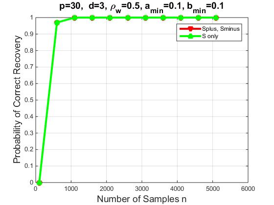
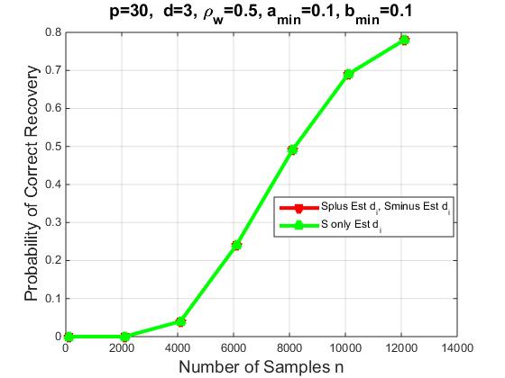
Fig. 2(a) assumes that for all and corresponds to comparing the described scheme in the second remark after Alg. 1 with an exhaustive learning algorithm, which selects as support for the sized neighborhood among all the neighborhoods with the maximum directed information flow to the th node. The proposed scheme has comparable performance with the aforementioned exhaustive observer, but with a significantly smaller computational complexity and comparable (and small) number of samples. In this plot, we compare only with respect to the selection of . The described scheme in the second remark after Alg. 1 can further discriminate between and . This is verified in Fig. 2(b) for a different setup. In Fig. 2(b), a single satisfying the BAR Identifiability Condition has been selected for all and for all again. Moreover, and . We note here that in practice there might be instances where the selection of is errorless, but the discrimination of and is erroneous for some of the rows.
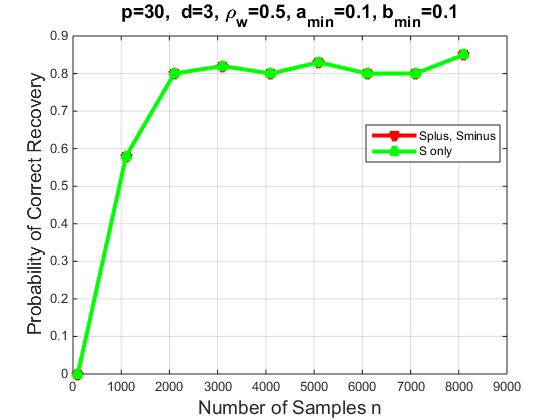
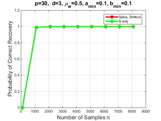
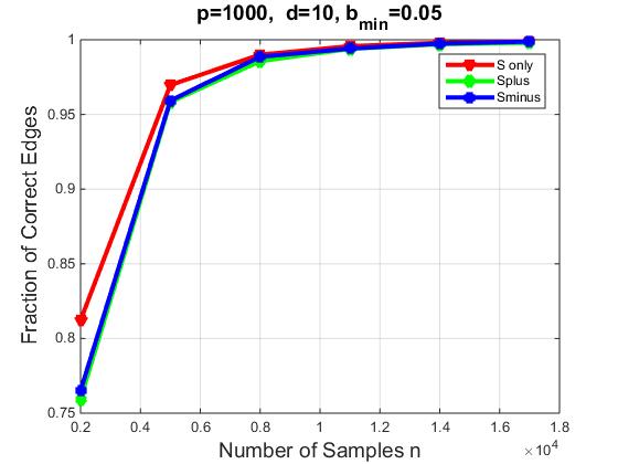
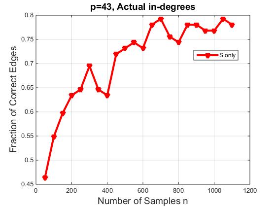
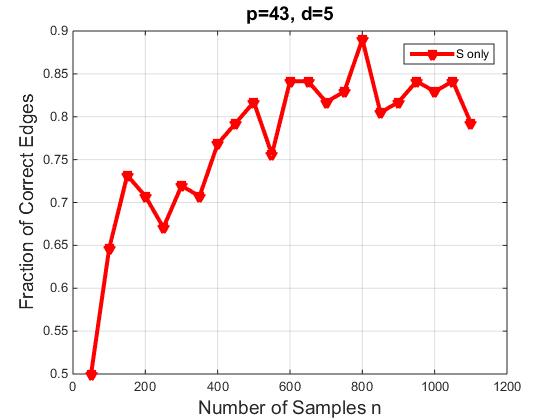
Remaining in the described scheme in the second remark after Alg. 1, Fig. 3(a) presents the scenario where all nodes have different but a priori known in-degrees and all the in-degrees are upper bounded by . To implicitly quantify what fraction of BAR chains with , and () satisfy the BAR Identifiability Condition or tends to create a larger amount of helpful than harmful correlations, we vary per run. We observe that approximately of the generated chains fall into this category leading to complete recovery with approximately samples. Fig. 3(b) shows that for a chain in this scenario, recovery can be achieved even with approximately samples. Additionally, since or are hard metrics in the sense that they correspond to the correct selection of parameters in , it is of interest to examine how many edges and orientations are correctly selected with an increasing number of samples, even when . To this end, Fig. 6(a) corresponds to the scenario and all nodes have the same in-degree . Clearly, a very large part of the true network is correctly selected fairly quickly. Note that the values of and in this scenario could be prohibitive for many previously studied model order selection methods. In this plot, “Fraction of Correct Edges” refers to what fraction of the true edges only the scheme identifies. Knowledge of the in-degrees and the fact that imply that the non-edges are also identified with very high probability. This is demonstrated in Fig. 6(b), which we describe later on.
Moving now to the described scheme in the first remark after Alg. 1, Fig. 4(a) presents the scenario where all nodes have different and unknown in-degrees and all the in-degrees are upper bounded by . In this case, the described scheme in the first remark after Alg. 1 will return a supergraph of the actual graph. Therefore, the axis corresponds to probability of correct recovery of a supergraph of the actual graph. To implicitly quantify what fraction of chains with and in-degree overestimate satisfies the BAR identifiability condition or tends to create a larger amount of helpful than harmful correlations, we vary per run. We observe that this plot does not differ significantly from Fig. 3(a) as expected, since the upper bound allows in many cases rows with exactly nonzero entries. Furthermore, Fig. 4(b) shows that for a matrix in the same scenario, recovery can be achieved with approximately samples. In practice, the minimum number of samples turns out to actually be . Comparing these results with Fig. 3(b), we can see that the outcome is in agreement with the fact that the described scheme in the first remark after Alg. 1 generates a supergraph of the actual graph, hence requiring less samples for complete recovery.
10.1.2 Complete BARObs
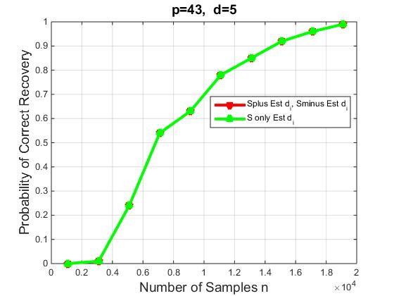
Fig. 5(a) presents the performance of BARObs in a scenario where all nodes have different and unknown in-degrees and all of the in-degrees are upper bounded by . In this case, the supergraph selection stage will return a supergraph of the actual graph and then the supergraph trimming stage will refine this estimate by estimating the in-degrees and the actual neighborhoods of each node. To implicitly quantify what fraction of chains with and satisfy the BAR Identifiability Condition or tends to create a larger amount of helpful than harmful correlations and what is the correspondence with respect to the BARObs in samples for perfect detection, we vary per run. Furthermore, Fig. 5(b) shows that for a matrix in the same scenario, recovery can be achieved with approximately samples. This is the price paid for the unknown ’s that have to be estimated.
10.2 Data from a Biological Signaling Network
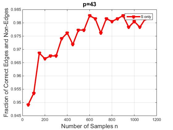
We use a publicly available model for an abscisic acid signaling network consisting of nodes provided in [20]. Each node is linked to a boolean rule defined by a subset of nodes in the network. We approximate the network in the spirit of BAR models. The approximation is not exactly the described BAR model but an appropriate version of the model for the boolean network at hand. We generate stochastic pseudodynamical data by adding binary/boolean noise to the produced time series. In Fig. 6(b), we plot the output of the algorithm in the second remark after Alg. 1. We observe that the supergraph selection only stage can identify almost of the true underlying network using only samples. Of course, the curve here is biased since we assume that we know exactly the in-degrees in this plot, hence the non-edges are correctly identified with high probability since the in-degrees are small. Moreover, the performance of this algorithm when we are only interested in the fraction of the actual edges correctly identified is depicted in Fig. 7(a). We also examine the performance of the algorithm described in the first remark after Alg. 1. Here, the goal is to evaluate what fraction of the actual edges we pick by a known overestimate . In Fig.7(b), and in Fig. 8(a), . We clearly see the improvement by using a larger . Finally, based on the same publicly available model for an abscisic acid signaling network, we create a noisy version of an AND/OR only network with and for all . We apply BAROBs and as Fig. 8(b) shows, we can identify the true network with probability when we have approximately time-series samples and with probability almost when we have samples.


11 Conclusions
In this paper, a novel model, called BAR, was introduced as an alternative to the description of binary vector random processes with autoregressive dynamics. BAR processes can be used to model opinion dynamics over social networks, voter processes, epidemics, interactions among stocks in financial markets and among genes or chemical elements in biological networks. We proved that the general BAR model mixes rapidly. We also showed that two random walk versions of this model mix rapidly under some conditions. Furthermore, we provided a low-complexity algorithm that can be used to identify the structure of the BAR network based on time-series data. This structure estimator was shown to be nearly order-optimal in sample complexity, adding new attractive features to the proposed BAR model.
A
Proof of Lemma 1
and depend on and , respectively. To ease the notation, we will write for and for in the remaining of this proof. We will further assume that any entropy is expressed using the natural logarithm, hence it is measured in nats.
For , we have the following well-known Taylor series expansion:
Therefore,
and a similar expression holds for . We can now see that
where in the last equality we have used the observation that and . Therefore, depends critically on .
B
Proof of Lemma 3
Given any vector norm , the induced operator norm for an matrix is defined as [18]:
where can be either or . On the other hand, if , the spectral radius of is defined as:
where are the eigenvalues of and is the complex modulus. For any it holds , while Gelfand’s formula states that for any matrix norm [18]:
When is symmetric or Hermitian, . In general, for any matrix norm .
For easiness, we will work with the Euclidean vector norm and the associated induced matrix norm, which is the spectral norm:
| (62) |
Here, and correspond to the maximum singular value and the maximum eigenvalue of a matrix, respectively. Moreover, stands for Hermitian transposition, which is for real ’s. Working in the following with and for any , (62) implies that the corresponding maximizing vectors for and correspond to the top eigenvectors of and , which are real vectors by basic facts in linear algebra.
In order to prove our claim, it is sufficient to show that for any . Consider first the case . Since has non-negative entries, it is clear that is maximized for with such that either for all or for all . Clearly, for any such , we have: . Consider now a with such that is maximized. If this has only non-negative or only non-positive entries, then . On the other hand, if contains some positive and some negative entries, then by inverting the polarities to either the positive or the negative entries, we end up with a such that and ; thus again . Note here, that the existence of non-positive and non-negative entries in leads to possible lower entries in magnitude in for rows containing only non-negative or only non-positive entries. The corresponding entries in will be larger in magnitude, which verifies our claim.
We can also extend the above argument in the complex field (although this extension is not required for the proof, but only for reasons of mathematical completeness). Consider for any such that . Then, we can form based on such that all real parts are co-signed and all imaginary parts are also co-signed (the signs in the real and imaginary parts can be different, e.g., all real parts can be positive and all imaginary parts can be negative). Then, and , which demonstrates the extension of the above argument in the complex field.
We now note that contains non-negative entries for any . On the other hand any entry in that does not coincide with the corresponding entry in , will be either negative and of the same magnitude, or negative and of smaller magnitude or positive and of smaller magnitude (i.e., the existence of negative elements in tend to have a contracting effect on the entries of as increases). Thus, by the same reasoning, for any . Using now Gelfand’s formula and taking the limit in both sides, we obtain:
Finally, we note that is a substochastic matrix and a straightforward application of Gershgorin’s Theorem yields that .
Proof of Lemma 4
By our assumptions:
Moreover,
Using the stability of , we have:
where we have used von Neumann’s series formula [19].
C
Proof of Corollary 1
Let . By an elementary argument,
To see that
we give the following counterexample. Consider the joint measure:
A straightforward calculation shows that
Finally, for :
D
Proof of Lemma 7
We would like to lower bound the number of required samples such that the worst case . Clearly, the number of required samples should be at least the number of required samples for for any valid choice of and . To this end, fixing and assuming that each with cardinality is drawn independently and uniformly at random, Fano’s inequality implies that
Consider the mutual information:
Replacing the LHS with
we obtain:
where for the term we have used the bound . Thus,
Using now the fact that and requiring that , we obtain:
where the term has been neglected.
E
Proof of Lemma 8
Assume that we populate randomly each row of with entries. Let’s describe the procedure:
-
1.
For each row, we pick independently one of the binary vectors with ones. This is the support of the respective row.
-
2.
At the locations of the ’s, we place the nonzero entries of this row of .
Clearly, the support of the th row is selected with probability
It is now easy to see, that each location in the th row vector has probability
of being selected. The numerator occurs if we fix a to the location of interest and we distribute the rest of the ones to the remaining positions at random.
Consider now the matrix , where for and otherwise. Thus, is the support matrix of with ’s at the nonzero locations and zeros elsewhere. Let be the column sums of this matrix. Each sum contains independent random variables as summands. By Hoeffding’s inequality:
or
Choosing for some positive constant , we obtain:
Using now the union bound, we have:
which goes to as for any . Thus, with probability at least ,
Proof of Lemma 9
Assume that we allow each non-zero entry of to be in the interval . Then, with probability at least
Requiring the rightmost handside to be , we obtain that
The rest of the claims follow from Theorem 6.
References
- Agaskar and Lu [2013] A. Agaskar and Y. M. Lu. Alarm: A logistic auto-regressive model for binary processes on networks. In Proceedings of GlobalSIP, December 2013.
- Aldous and Vazirani [1990] D. Aldous and U. Vazirani. A Markovian extension of Valiant’s learning model. In FOCS, 1990.
- Anandkumar et al. [2012a] A. Anandkumar, V. Y. F. Tan, F. Huang, and A. S. Willsky. High-dimensional structure estimation in ising models: Local separation sriterion. The Annals of Statistics, 40(3):1346–1375, 2012a.
- Anandkumar et al. [2012b] A. Anandkumar, V. Y. F. Tan, and A. S. Willsky. High-dimensional gaussian graphical model selection: Walk summability and local separation criterion. Journal of Machine Learning Research, 13(1):2293–2337, 2012b.
- Barrat et al. [2008] A. Barrat, M. Barthelemy, and A. Vespignani. Dynamical Processes on Complex Networks. Cambridge University Press, 2008.
- Bartlett et al. [1994] P. L. Bartlett, P. Fischer, and K.-U. Höffgen. Exploiting random walks for learning. In COLT, 1994.
- Bento et al. [2010] J. Bento, M. Ibrahimi, and A. Montanari. Learning networks of stochastic differential equations. In NIPS, Vancouver, B.C., Canada, Dec. 2010.
- Bolstad et al. [2011] A. Bolstad, B. Van Veen, and R. Nowak. Causal network inference via group sparse regularization. IEEE Trans. on Signal Processing, 59(6):2628–2641, 2011.
- Bresler [2015] G. Bresler. Efficient learning ising models on arbitrary graphs. In Symposium on Theory of Computing (STOC), 2015.
- Bresler et al. [2014] G. Bresler, D. Gamarnik, and D. Shah. Learning graphical models from the glauber dynamics. In Proceedings of Allerton, 2014.
- Bubley and Dyer [1997] R. Bubley and M. Dyer. Path coupling: A technique for proving rapid mixing in markov chains. In Annual Symposium on Foundations of Computer Science (FOCS), 1997.
- Chatterjee et al. [2013] A. Chatterjee, A. S. Rawat, S. Vishwanath, and S. Sanghavi. Learning the causal graph of markov time series. In Proceedings of Allerton, 2013.
- Chow and Liu [1968] C. Chow and C. Liu. Approximating discrete probability distributions with dependence trees. IEEE Transactions on Information Theory, 14(3):462–467, 1968.
- Chung et al. [2012] K-M. Chung, H. Lam, Z. Liu, and M. Mitzenmacher. Chernoff-hoeffding bounds for markov chains: Generalized and simplified. In Symposium on Theoretical Aspects of Computer Science (STACS), 2012.
- Gamarnik [2003] D. Gamarnik. Extension of the PAC framework to finite and countable Markov chains. IEEE Trans. on Inf. Theory, 49(1):338–345, 2003.
- Goodwin and Payne [1977] G. C. Goodwin and R. L. Payne. Dynamic System Identification: Experiment Design and Data Analysis. Academic Press, 1977.
- Granger [1969] C. W. J. Granger. Investigating causal relations by econometric models and cross-spectral methods. Econometrica, 37(3):424–438, 1969.
- Horn and Johnson [1985] R. A. Horn and C. R Johnson. Matrix Analysis. Cambridge University Press, 1985.
- Horn and Johnson [1991] R. A. Horn and C. R Johnson. Topics in Matrix Analysis. Cambridge University Press, 1991.
- [20] J. W. Jenkins and A. Soni. Abscisic acid signaling network. available at: http://www.causality.inf.ethz.ch/repository.php?id=5.
- Kramer [1998] G. Kramer. Directed Information for Channels with Feedback. ETH Series in Inf. Proc., 1998.
- Kramer [2003] G. Kramer. Capacity results for the discrete memoryless network. IEEE Trans. on Information Theory, 49:4–21, 2003.
- Levin et al. [2008] D. A. Levin, Y. Peres, and E. L. Wilmer. Markov Chains and Mixing Times. American Mathematical Society, 2008.
- Ljung [1999] L. Ljung. System Identification-Theory For the User. Prentice Hall, Upper Saddle River, New Jersey, 1999.
- Marko [1973] H. Marko. Capacity results for the discrete memoryless network. IEEE Trans. on Comm., COM-21:1345–1351, 1973.
- Massey [1990] J. L. Massey. Causality, feedback and directed information. In Int. Symp. on Inf. Theory and its Appls., Hawaii, USA, Nov. 1990.
- Materassi et al. [2013] D. Materassi, G. Innocenti, L. Giarré, and M. V. Salapaka. Model identification of a network as compressing sensing. Systems & Control Letters, 62(8):664–672, 2013.
- Myers and Leskovec [2010] S. Myers and J. Leskovec. On the convexity of latent social network inference. In NIPS, 2010.
- Netrapalli and Sanghavi [2012] P. Netrapalli and S. Sanghavi. Learning the graph of epidemic cascades. In SIGMETRICS, 2012.
- Quinn et al. [2015] C. J. Quinn, N. Kiyavash, and T. P. Coleman. Directed information graphs. IEEE Trans. on Information Theory, 61(12):6887–6909, 2015.
- Rodriguez et al. [2011] M. G. Rodriguez, D. Balduzzi, and B. Schölkopf. Uncovering the temporal dynamics of diffusion networks. arXiv:1105.0697, 2011.
- Rosenthal [1995] J. S. Rosenthal. Convergence rates for markov chains. SIAM Review, 37(3):387–405, 1995.
- Santhanam and Wainwright [2012] N. P. Santhanam and M. J. Wainwright. Information-theoretic limits of selecting binary graphical models in high dimensions. IEEE Trans. on Inf. Theory, 58(7):4117–4134, 2012.
- Sun et al. [2015] J. Sun, D. Taylor, and E. M. Bollt. Causal network inference by optimal causation entropy. arXiv:1401.7574, 2015.
- Wainwright [2015] M. J. Wainwright. Graphical Models and Message passing algorithms: Some introductory lectures. Lecture Notes in Mathematics, Springer, 2015.
- Wasserman and Roeder [2009] L. Wasserman and K. Roeder. High-dimensional variable selection. The Annals of Statistics, 37(5A):2178–2301, 2009.
- Zhao and Yu [2006] P. Zhao and B. Yu. On model selection consistency of lasso. Journal of Machine Learning Research, 7:2541–2563, 2006.