Sensitivity of Fields Generated within Magnetically Shielded Volumes to Changes in Magnetic Permeability

Abstract

Future experiments seeking to measure the neutron electric dipole moment (nEDM) require stable and homogeneous magnetic fields. Normally these experiments use a coil internal to a passively magnetically shielded volume to generate the magnetic field. The stability of the magnetic field generated by the coil within the magnetically shielded volume may be influenced by a number of factors. The factor studied here is the dependence of the internally generated field on the magnetic permeability $\mu$ of the shield material. We provide measurements of the temperature-dependence of the permeability of the material used in a set of prototype magnetic shields, using experimental parameters nearer to those of nEDM experiments than previously reported in the literature. Our measurements imply a range of $\frac{1}{\mu}\frac{d\mu}{dT}$ from 0-2.7%/K. Assuming typical nEDM experiment coil and shield parameters gives $\frac{\mu}{B_{0}}\frac{dB_{0}}{d\mu}=0.01$, resulting in a temperature dependence of the magnetic field in a typical nEDM experiment of $\frac{dB_{0}}{dT}=0-270$ pT/K for $B_{0}=1~{}\mu$T. The results are useful for estimating the necessary level of temperature control in nEDM experiments.

1 Introduction

The next generation of neutron electric dipole moment (nEDM) experiments aim to measure the nEDM $d_{n}$ with proposed precision $\delta d_{n}\lesssim 10^{-27}~{}e\cdot$cm [1, 2, 3, 4, 5, 6, 7, 8]. In the previous best experiment [9, 10] which discovered $d_{n}<3.0\times 10^{-26}~{}e\cdot$cm (90% C.L), effects related to magnetic field homogeneity and instability were found to dominate the systematic error. A detailed understanding of passive and active magnetic shielding, magnetic field generation within shielded volumes, and precision magnetometry is expected to be crucial to achieve the systematic error goals for the next generation of experiments. Much of the research and development efforts for these experiments are focused on careful design and testing of various magnetic shield geometries with precision magnetometers [11, 12, 13, 14, 15].

In nEDM experiments, the spin-precession frequency $\nu$ of neutrons placed in static magnetic $B_{0}$ and electric $E$ fields is measured. The measured frequencies for parallel $\nu_{+}$ and antiparallel $\nu_{-}$ relative orientations of the fields is sensitive to the neutron electric dipole moment $d_{n}$

$$h\nu_{\pm}=2\mu_{n}B_{0}\pm 2d_{n}E$$ (1)

where $\mu_{n}$ is the magnetic moment of the neutron.

A problem in these experiments is that if the magnetic field $B_{0}$ drifts over the course of the measurement period, it degrades the statistical precision with which $d_{n}$ can be determined. If the magnetic field over one measurement cycle is determined to $\delta B_{0}=10$ fT, it implies an additional statistical error of $\delta d_{n}\sim 10^{-26}~{}e\cdot$cm (assuming an electric field of $E=10$ kV/cm which is reasonable for a neutron EDM experiment). Over 100 days of averaging, this would make a $\delta d_{n}\sim 10^{-27}~{}e\cdot$cm measurement possible. Unfortunately the magnetic field in the experiment is never stable to this level. For this reason, experiments use a comagnetometer and/or surrounding atomic magnetometers to measure and correct the magnetic field to this level [9, 11, 12]. Drifts of 1-10 pT in $B_{0}$ may be corrected using the comagnetometer technique, setting a goal magnetic stability for the $B_{0}$ field generation system in a typical nEDM experiment.

In such experiments, typically $B_{0}=1~{}\mu$T is used to provide the quantization axis for the ultracold neutrons. The $B_{0}$ magnetic field generation system typically includes a coil placed within a passively magnetically shielded volume. The passive magnetic shield is generally composed of a multi-layer shield formed from thin shells of material with high magnetic permeability (mu-metal). The outer layers of the shield are normally cylindrical [1, 4] or form the walls of a magnetically shielded room [16, 17]. The innermost magnetic shield is normally a specially shaped shield, where the design of the coil in relation to shield is carefully taken into account to achieve adequate homogeneity [9, 3, 5].

Mechanical and temperature changes of the passive magnetic shielding [18, 19], and the degaussing procedure [19, 17, 20] (also known as demagnetization, equilibration, or idealization), affect the stability of the magnetic field within magnetically shielded rooms. Active stabilization of the background magnetic field surrounding magnetically shielded rooms can also improve the internal stability [18, 12, 21]. The current supplied to the $B_{0}$ coil is generated by an ultra-stable current source [11]. The coil must also be stabilized mechanically relative to the magnetic shielding.

One additional effect, which is the subject of this paper, relates to the fact that the $B_{0}$ coil in most nEDM experiments is magnetically coupled to the innermost magnetic shield. If the magnetic properties of the innermost magnetic shield change as a function of time, it then results in a source of instability of $B_{0}$. In the present work, we estimate this effect and characterize one possible source of instability: changes of the magnetic permeability $\mu$ of the material with temperature.

While the sensitivity of magnetic alloys to temperature variations has been characterized in the past [22, 23], we sought to make these measurements in regimes closer to the operating parameters relevant to nEDM experiments. For these alloys, it is also known that the magnetic properties are set during the final annealing process [24, 25, 23]. In this spirit we performed our measurements on “witness” cylinders, which are small open-ended cylinders made of the same material and annealed at the same time as other larger shields are being annealed.

The paper proceeds in the following fashion:

• The dependence of the internal field on magnetic permeability of the innermost shielding layer for a typical nEDM experiment geometry is estimated using a combination of analytical and finite element analysis techniques. This sets a scale for the stability problem.

• New measurements of the temperature dependence of the magnetic permeability are presented. The measurements were done in two ways in order to study a variety of systematic effects that were encountered.

• Finally, the results of the calculations and measurements are combined to provide a range of temperature sensitivities that takes into account sample-to-sample and measurement-to-measurement variations.

2 Sensitivity of Internally Generated Field to Permeability of the Shield $B_{0}(\mu)$

The presence of a coil inside the innermost passive shield turns the shield into a return yoke, and generally results in an increase in the magnitude of $B_{0}$. The ratio of this field inside the coil in the presence of the magnetic shield to that of the coil in free space is referred to as the reaction factor $C$, and can be calculated analytically for spherical and infinite cylindrical geometries [26, 27]. The key issue of interest for this work is the dependence of the reaction factor on the permeability $\mu$ of the innermost shield. Although this dependence can be rather weak, the constraints on $B_{0}$ stability are very stringent. As a result, even a small change in the magnetic properties of the innermost shield can result in an unacceptably large change in $B_{0}$.

To illustrate, we consider here the model of a sine-theta surface current on a sphere of radius $a$, inside a spherical shell of inner radius $R$, thickness $t$, and linear permeability $\mu$. The uniform internal field generated by this ideal spherical coil is augmented by the reaction factor in the presence of the shield, but is otherwise left undistorted. The general reaction factor for this model is given by Eq. (38) in Ref. [26]. In the high-$\mu$ limit, with $t\ll R$, the reaction factor can be approximated as

$$C\simeq 1+\frac{1}{2}\,\left(\frac{a}{R}\right)^{3}\left(1-\frac{3}{2}\,\frac{R}{t}\,\frac{\mu_{\scriptscriptstyle 0}}{\mu}\right)\,,$$ (2)

which highlights the dependence of $B_{0}$ on the relative permeability $\mu_{r}=\mu/\mu_{\scriptscriptstyle 0}$ of the shield.

Fig. 1 (upper) shows a plot of $B_{0}$ versus $\mu_{r}$ for coil and shield dimensions similar to the ILL nEDM experiment [9, 28]: $a=0.53$ m, $R=0.57$ m, and $t=1.5$ mm. In addition to analytic calculations, we also include the results of two axially symmetric simulations conducted using FEMM [29] to assess the effects of geometry and discretization of the surface current. The differences are small, suggesting that the ideal spherical model of Ref. [26] and the high-$\mu$ approximation of Eq. 2 provide valuable insight for the design and analysis of shield-coupled coils.

Figure 1: Upper: Magnetic field at the coil center as a function of magnetic permeability of the surrounding magnetic shield for a geometry similar to the ILL nEDM experiment as discussed in the text. Lower: $\frac{\mu}{B_{0}}\frac{dB_{0}}{d\mu}$ vs. permeability. The solid curve is the exact calculation for the ideal spherical coil and shield from Ref. [26]; the dashed curve is the approximation of Eq. 2. The circles and squares are the FEMM-based simulations for the spherical and solenoidal geometries with discrete currents. Since the spherical simulation was in agreement with the calculation, it is omitted from the lower graph. For the exact calculation and the two simulations, currents were chosen to give $B_{0}=1~{}\mu$T at $\mu_{r}=20,000$.

In the first simulation, the same spherical geometry was used as for the analytic calculations. However, the surface current was discretized to 50 individual current loops, inscribed onto a sphere, and equally spaced vertically (i.e. a discrete sine-theta coil). A square wire profile of side length 1 mm was used. As shown in Fig. 1, this simulation gave excellent agreement with the analytic calculations. In the second simulation, a solenoid coil and cylindrical shield (length/radius = 2) were used with the same dimensions as above. Similarly, the coil was modelled as 50 evenly spaced current loops, with the distance from an end loop to the inner face of the shield endcap being half the inter-loop spacing. In the limit of tight-packing (i.e., a continuous surface current) and infinite $\mu$, the image currents in the end caps of the shield act as an infinite series of current loops, giving the ideal uniform field of an infinitely long solenoid [30, 31]. As shown in Fig. 1, the result is similar to the spherical case, with differences of order one part per thousand and a somewhat steeper slope of $B_{0}(\mu_{r})$.

Fig. 1 (lower) shows the normalized slope $\frac{\mu}{B_{0}}\frac{dB_{0}}{d\mu}$ of the curves from Fig. 1 (upper). In ancillary measurements of shielding factors (discussed briefly in Section 3.1), we found $\mu_{r}=20,000$ to offer a reasonable description of the quasistatic shielding factor of our shield. Using this value as the magnetic permeability of our shield material, Fig. 1 (lower) shows that $\frac{\mu}{B_{0}}\frac{dB_{0}}{d\mu}$ varies by about 20% (from 0.008 to 0.01) for the spherical vs. solenoidal geometries. We adopt the value $\frac{\mu}{B_{0}}\frac{dB_{0}}{d\mu}=0.01$ as an estimate of this slope in our discussions in Section 4, acknowledging that the value depends on the coil and shield design.

For a high-$\mu$ innermost shield, the magnetic field lines emanating from the coil all return through the shield. This principle can be used to estimate the magnetic field $B_{m}$ inside the shield material, and in our studies gave good agreement with FEA-based simulations. For the solenoidal geometry previously described and used for the calculations in Fig. 1, $B_{m}$ is largest in the side walls of the solenoidal flux return, attaining a maximum value of 170 $\mu$T. If we assume $\mu_{r}$=20,000, the $H_{m}$ field is 0.007 A/m. Typically the shield is degaussed (idealized) with the internal coil energized. After degaussing, $B_{m}$ must be approximately the same, since essentially all flux returns through the shield. However, the $H_{m}$ field may become significantly smaller because after degaussing, it must fall on the ideal magnetization curve in $B_{m}-H_{m}$ space. (For a discussion of the ideal magnetization curve, we refer the reader to Ref. [25].) In principle, the $H_{m}$ field could be reduced by an order of magnitude or more, depending on the steepness of the ideal magnetization curve near the origin. Thus $B_{m}=170~{}\mu$T and $H_{m}<0.007$ A/m set a scale for the relevant values for nEDM experiments. Furthermore, the field in the nEDM measurement volume, as well as in the magnetic shield, must be stable for periods of typically hundreds of seconds (corresponding to frequencies $<0.01$ Hz). This sets the relevant timescale for magnetic properties most relevant to nEDM experiments.

3 Measurements of $\mu(T)$

3.1 Previous Measurements and their Relationship to nEDM Experiments

Previous measurements of the temperature dependence of the magnetic properties of high-permeability alloys have been summarized in Refs. [22, 25, 32]. These measurements are normally conducted using a sample of the material to create a toroidal core, where a thin layer of the material is used in order to avoid eddy-current and skin-depth effects [32, 23]. A value of $\mu$ is determined by dividing the amplitude of the sensed $B_{m}$-field by the amplitude of the driving AC $H_{m}$-field (similar to the method described in Section 3.3). Normally the frequency of the $H_{m}$-field is 50 or 60 Hz. The value of $\mu$ is then quoted either at or near its maximum attainable value by adjusting the amplitude of $H_{m}$. Depending on the details of the $B_{m}-H_{m}$ curve for the material in question, this normally means that $\mu$ is quoted for the amplitude of $H_{m}$ being at or near the coercivity of the material [22, 23], resulting in large values up to $\mu_{r}=4\times 10^{5}$.

It is well known that $\mu$ measured in this fashion for toroidal, thin metal wound cores depends on the annealing process used for the core. There is a particularly strong dependence on the take-out or tempering temperature after the high-temperature portion of the annealing process has been completed [32, 23, 22]. Such studies normally suggest a take-out temperature of 490-500^∘C. This ensures that the large $\mu_{r}=4\times 10^{5}$ is furthermore maximal at room temperature. Slight variations around room temperature, and assuming the take-out temperature is not controlled to better than a degree, imply a scale of possible temperature variation of $\mu$ of approximately $\left|\frac{1}{\mu}\frac{d\mu}{dT}\right|\simeq 0.3$-1%/K at room temperature [22, 23].

A challenge in applying these results to temperature stability of nEDM experiments is that, when used as DC magnetic shielding, the high-permeability alloys are usually operated for significantly different parameters ($B_{m}$, $H_{m}$, and frequencies).

For example, when used in a shielding configuration, the effective permeability is often measured to be typically $\mu_{r}=20,000$ rather than $4\times 10^{5}$. This arises in part because $H_{m}$ is well below the DC coercivity. As noted in Section 2, a more appropriate $H_{m}$ for the innermost magnetic shield of an nEDM experiment is $<0.007$ A/m, whereas the coercivity is $H_{c}=0.4$ A/m [23]. The frequency dependence of the measurements could also be an issue. Typically, nEDM experiments are concerned with slow drifts at $<0.01$ Hz timescales whereas the previously reported $\mu(T)$ measurements are performed in an AC mode at 50-60 Hz.

The goal of our experiments was to develop techniques to characterize the material properties of our own magnetic shields post-annealing, in regimes more relevant to nEDM experiments.

We created a prototype passive magnetic shield system in support of this and other precision magnetic field research for the future nEDM experiment to be conducted at TRIUMF. The shield system is a four-layer mu-metal shield formed from nested right-circular cylindrical shells with endcaps. The inner radius of the innermost shield is 18.44 cm, equal to its half-length. The radii and half-lengths of the progressively larger outer shields increase geometrically by a factor of 1.27. Each cylinder has two endcaps which possess a 7.5 cm diameter central hole. A stove-pipe of length 5.5 cm is placed on each hole was designed to minimize leakage of external fields into the progressively shielded inner volumes. The design is similar to another smaller prototype shield discussed in Ref. [33]. The magnetic shielding factors of each of the four cylindrical shells, and of various combinations of them, were measured and found to be consistent with $\mu_{r}\sim 20,000$.

In our studies of the material properties of these magnetic shields, two different approaches to measure $\mu(T)$ were pursued. Both approaches involved experiments done using witness cylinders made of the same material and annealed at the same time as the prototype magnetic shields. We therefore expect they have the same magnetic properties as the larger prototype shields, and they have the advantage of being smaller and easier to perform measurements with.

The two techniques employed to determine $\mu(T)$ were the following:

1. measuring the low-frequency AC axial magnetic shielding factor of the witness cylinder as a function of temperature, and

2. measuring the temperature-dependence of the slope of a minor B-H loop, using the witness cylinder as a transformer core, similar to previous measurements of the temperature dependence of $\mu$, but for parameters closer to those encountered in nEDM experiments.

We now discuss the details and results of each technique.

3.2 Axial Shielding Factor Measurements

In these measurements, a witness cylinder was used as a magnetic shield. The shield was subjected to a low-frequency AC magnetic field of $\sim 1$ Hz. The amplitude of the shielded magnetic field $B_{s}$ was measured at the center of the witness cylinder using a fluxgate magnetometer. Changes in $B_{s}$ with temperature signify a dependence of the permeability $\mu$ on temperature. The relative slope of $\mu(T)$ can then be calculated using

$$\frac{1}{\mu}\frac{d\mu}{dT}=-\frac{\frac{1}{B_{s}}\frac{dB_{s}}{dT}}{\frac{\mu}{B_{s}}\frac{dB_{s}}{d\mu}}.$$ (3)

The numerator was taken from the measurements described above. The denominator was taken from finite-element simulations of the shielding factor for this geometry as a function of $\mu$.

This measurement technique was sufficiently robust to extract the temperature dependence of the shielding factor with some degree of certainty. Possible drifts and temperature depends of the fluxgate magnetometer offset were mitigated by using an AC magnetic field. Any temperature coefficients in the rest of the instrumentation were controlled by performing the same measurements with a copper cylindrical shell in place of the mu-metal witness cylinder.

This technique is quite different than the usual transformer core measurements conducted by other groups. As shall be described, it offers an advantage that considerably smaller $B_{m}$ and $H_{m}$ fields can be accessed. Measuring the temperature dependence of the shielding factor is also considerably easier than measuring the temperature dependence of the reaction factor, since the sensitivity to changes in $\mu(T)$ is considerably larger in magnitude for the shielding factor case where $\frac{\mu}{B_{s}}\frac{dB_{s}}{d\mu}\sim-1$ compared to the reaction factor case where $\frac{\mu}{B_{0}}\frac{dB_{0}}{d\mu}\sim 0.01$.

3.2.1 Experimental Apparatus for Axial Shielding Factor Measurements

The witness cylinder was placed within a homogeneous AC magnetic field. The field was created within the magnetically shielded volume of the prototype magnetic shielding system (described previously in Section 3.1) in order to provide a controlled magnetic environment. A short solenoid inside the shielding system was used to produce the magnetic field. The solenoid has 14 turns with 2.6 cm spacing between the wires. The solenoid was designed so that the field produced by the solenoid plus innermost shield approximates that of an infinite solenoid. The magnetic field generated by the solenoid was typically 1 $\mu$T in amplitude. The solenoid current was varied sinusoidally at typically 1 Hz.

The witness cylinder was placed into this magnetic field generation system as shown schematically in Fig. 2. The cylinder was held in place by a wooden stand.

A Bartington fluxgate magnetometer Mag-03IEL70 [34] (low noise) measured the axial magnetic field at the center of the witness cylinder. The fluxgate was a “flying lead” model, meaning that each axis was available on the end of a short electrical lead, separable from the other axes. One flying lead was placed in the center of the witness cylinder, the axis of the fluxgate being aligned with that of the witness cylinder. The fluxgate was held in place rigidly by a plastic mounting fixture, which was itself rigidly mounted to the witness cylinder.

To increase the resolution of the measured signal from the fluxgate, a Bartington Signal Conditioning Unit (SCU) was used with a low-pass filter set to typically 10-100 Hz and a gain set to typically $>50$. The signal from the SCU was demodulated by an SR830 lock-in amplifier [35] providing the in-phase and out-of-phase components of the signal. The sinusoidal output of the lock-in amplifier reference output itself was normally used to drive the solenoid generating the magnetic field. The time constant on the lock-in was typically set to 3 seconds with 12 dB/oct rolloff.

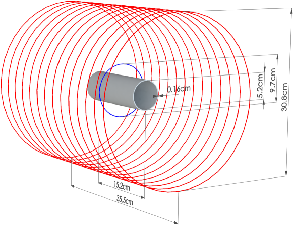
Figure 2: (color online) Axial shielding factor measurement setup. The witness cylinder with an inner diameter of 5.2 cm and a length of 15.2 cm is placed inside a solenoid (shown in red) with a diameter of 30.8 cm and a length of 35.5 cm, containing 14 turns. The thickness of the witness cylinder is $1/16^{\prime\prime}=0.16$ cm. The loop coil (shown in blue) is mechanically coupled to the witness cylinder and has a diameter of 9.7 cm.

As shall be described in Section 3.2.2, a concern in the measurement was changes in the field measured by the fluxgate that could arise due to motion of the system components, or other temperature dependences. This could generate a false slope with temperature that might incorrectly be interpreted as a change in the magnetic properties of the witness cylinder.

To address possible motion of the witness cylinder with respect to the field generation system, another coil (the loop coil, also shown in Fig. 2) was wound on a plastic holder mounted rigidly to the witness cylinder. The coil was one loop of copper wire with a diameter of 9.7 cm. Plastic set screws in the holder fixed the loop coil to be coaxial with the witness cylinder.

Systematic differences in the results from the two coils (the solenoidal coil, and the loop coil) were used to search for motion artifacts. As well, some differences could arise due to the different magnetic field produced by each coil, and so such measurements could reveal a dependence on the profile of the applied magnetic field. This is described further in Section 3.2.2.

The temperature of the witness cylinder was measured by attaching four thermocouples at different points along the outside of the cylinder. This allowed us to observe the temperature gradient along the witness cylinder. To reduce any potential magnetic contamination, T-type thermocouples were used, which have copper and constantan conductors. (K-type thermocouples are magnetic.)

Thermocouple readings were recorded by a National Instruments NI-9211 temperature input module. The magnetic field (signified by the lock-in amplifier readout) and the temperature were recorded at a rate of 0.2 Hz.

Temperature variations in the experiment were driven by ambient temperature changes in the room, although forced air and other techniques were also tested. These are described further in Section 3.2.2.

3.2.2 Data and Interpretation

An example of the typical data acquired is shown in Fig. 3. For these data, the field applied by the solenoid coil was 1 $\mu$T in amplitude, at a frequency of 1 Hz. Fig. 3(a) shows the temperature of the witness cylinder over a 70-hr measurement. The temperature changes of 1.4 K are caused by diurnal variations in the laboratory. The shielded magnetic field amplitude $B_{s}$ within the witness cylinder is anti-correlated with the temperature trend as shown in Fig. 3(b). Here, $B_{s}$ is the sum in quadrature of the amplitudes of the in-phase and out-of-phase components (most of the signal is in phase). The magnetic field is interpreted to depend on temperature, and the two quantities are graphed as a function of one another in Fig. 3(c). The slope in Fig. 3(c) has been calculated using a linear fit to the data. The relative slope at 23^∘C was found to be $\frac{1}{B_{s}}\frac{dB_{s}}{dT}=-0.75\%$/K.

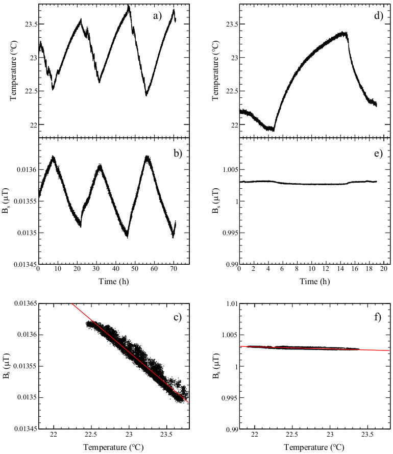
Figure 3: Ambient temperature and shielded magnetic field amplitude, measured over a 70 hour period. (a) temperature of the witness cylinder as a function of time. (b) magnetic field amplitude measured by fluxgate at center of witness cylinder vs. time. (c) magnetic field vs. temperature with linear fit to data giving $\frac{1}{B_{s}}\frac{dB_{s}}{dT}=-0.75\%$/K (evaluated at 23^∘C). In panels (d), (e), and (f), the same quantities are shown for a 20-hour run with a copper cylinder in place of the witness cylinder with the linear fit giving $\frac{1}{B_{s}}\frac{dB_{s}}{dT}=-0.03\%$/K.

Figs. 3(d), (e), and (f) show the same measurement with essentially the same settings, when the mu-metal witness cylinder is replaced by a copper cylinder. A similar relative vertical scale has been used in Figs. 3(e) and (f) as Figs. 3(b) and (c). This helps to emphasize the considerably smaller relative slope derived from panel (f) compared to panel (c). A variety of measurements of this sort were carried out multiple times for different parameters such as coil current. Running the coil at the same current tests for effects due to heating of the coil, whereas running the coil at a current which equalizes the fluxgate signal to its value when the mu-metal witness cylinder is present tests for possible effects related to the fluxgate. For all measurements the temperature dependence of the demodulated magnetic signal was $<0.1$%/K, giving confidence that unknown systematic effects contribute below this level.

Some deviations from the linear variation of $B_{s}$ with $T$ can be seen in the data, particularly in Figs. 3(a), (b), and (c). For example, when the temperature changes rapidly, the magnetic field takes some time to respond, resulting in a slope in $B_{s}-T$ space that is temporarily different than when the temperature is slowly varying. This is typical of the data that we acquired, that the data would generally follow a straight line if the temperature followed a slow and smooth dependence with time, but the data would not be linear if the temperature varied rapidly or non-monotonically with time. We also tried other methods of temperature control, such as forced air, liquid flowing through tubing, and thermo-electric coolers. The diurnal cycle driven by the building’s air conditioning system gave the most stable method of control and the most reproducible results for temperature slopes.

As mentioned earlier, data were acquired for both the solenoid coil and the loop coil. A summary of the data is provided in Table 1. Repeated measurements of temperature slopes using the loop coil fell in the range 0.4%/K $<|\frac{1}{B_{s}}\frac{dB_{s}}{dT}|<$ 1.5%/K. Similar measurements for the solenoidal coil yielded 0.3%/K $<|\frac{1}{B_{s}}\frac{dB_{s}}{dT}|<$ 0.8%/K.

Trial	$\frac{1}{B_{s}}\frac{dB_{s}}{dT}$	Coil
#	(%/K)	type
1	-0.32	solenoid
2	-0.30	solenoid
3	-0.33	solenoid
4	-1.53	loop
5	-0.42	loop
6	-1.30	loop
7	-0.74	solenoid
8	-1.05	loop
9	-0.73	solenoid
10	-1.23	loop
11	-0.75	solenoid
12	-1.12	loop

Table 1: Summary of data acquired for the AC axial shielding factor measurements, in chronological order. Data with an applied field of $\sim 1-6\mu T$ and a measurement frequency of 1 Hz are included. Data which used daily fluctuations of the temperature from 21-24^∘C over a 10-80 hour period are included. Other data acquired for systematic studies are not included in the table.

In general, the slopes measured with the loop coil were larger than for the solenoidal coil. This is particularly evident for measurements 6-12, which were acquired daily over the course of a few weeks alternating between excitation coils but all used the same witness cylinder and otherwise without disturbing the measurement apparatus. A partial explanation of this difference is offered by the field profile generated by each coil, and its interaction with the witness cylinder. This is addressed further in Section 3.2.3.

The other difference between the loop coil and the solenoidal coil was that the loop coil was rigidly mounted to the witness cylinder, reducing the possibility of artifacts from relative motion. Given that this did not reduce the range of the measured temperature slopes we conclude that relative motion was well controlled in both cases.

Several other possible systematic effects were considered, all of which were found to give uncertainties on the measured slopes $<0.1\%$/K. These included: thermal expansion of components including the witness cylinder itself, temperature variations of the magnetic shielding system within which the experiments were conducted, degaussing of the witness cylinder, and temperature slopes of various components e.g. the fluxgate magnetometer and the lock-in amplifier.

As mentioned earlier in reference to Fig. 3(d), (e), and (f), the stability of the system was also tested by replacing the mu-metal witness cylinder with a copper cylinder and in all cases temperature slopes $<0.1$%/K were measured, giving confidence that other unknown systematic effects contribute below this level.

Based on the systematic effects that we studied, we conclude that they do not explain the ranges of values measured for $\frac{1}{B_{s}}\frac{dB_{s}}{dT}$. We suspect that the range measured is either some yet uncharacterized systematic effect, or a complicated property of the material. We use this range to set a limit on the slope of $\mu(T)$

3.2.3 Geometry correction and determination of $\mu(T)$

To relate the data on $B_{s}(T)$ to $\mu(T)$, the shielding factor of the witness cylinder as a function of $\mu$ must be known. Finite element simulations in FEMM and OPERA were performed to determine this factor. The simulations are also useful for determining the effective values of $B_{m}$ and $H_{m}$ in the material, which will be useful to compare to the case for typical nEDM experiments when the innermost shield is used as a flux return.

For closed objects, such as spherical shells [26, 27], the shielding factor approaches infinity as $\mu\rightarrow\infty$, and $|\frac{\mu}{B_{s}}\frac{dB_{s}}{d\mu}|\rightarrow 1$. Because the witness cylinders are open ended, the shielding factor asymptotically approaches a constant rather than infinity in the high-$\mu$ limit, and as a result $|\frac{\mu}{B_{s}}\frac{dB_{s}}{d\mu}|<1$ here. From the simulations the ratio $\frac{\mu}{B_{s}}\frac{dB_{s}}{d\mu}$ was calculated. A linear model of the material was used where $\mathbb{B_{m}}=\mu\mathbb{H_{m}}$ with $\mu$ constant.

The simulations differed slightly in their results, dependent on whether OPERA or FEMM was used, and whether the solenoidal coil or loop coil were used. Based on the simulations, the result is $|\frac{\mu}{B_{s}}\frac{dB_{s}}{d\mu}|=0.42-0.50$ for the solenoidal coil, with the lower value being given by FEMM and the upper value being given by a 3D OPERA simulation, for identical geometries. This is somewhat lower than the value suggested by Ref. [36] with fits to simulations performed in OPERA, which we estimate to be 0.6. We adopt our value since it is difficult to determine precisely from Ref. [36]. For the loop coil, we determine $|\frac{\mu}{B_{s}}\frac{dB_{s}}{d\mu}|=0.56-0.65$, the range being given again by a difference between FEMM and OPERA.

Combining the measurement and the simulations, the temperature dependence of the effective $\mu$ (at $\mu_{r}=20,000$ which is consistent with our measurements) can be calculated by equation (3). The results of the simulations and measurements are presented in Table 2. Combining the loop coil and solenoidal coil results, we find 0.6%/K $<\frac{1}{\mu}\frac{d\mu}{dT}<2.7\%$/K to represent the full range for the possible temperature slope of $\mu$ that observed in these measurements.

	$|\frac{\mu}{B_{s}}\frac{dB_{s}}{d\mu}|$	$|\frac{1}{B_{s}}\frac{dB_{s}}{dT}|$ (%/K)	$\frac{1}{\mu}\frac{d\mu}{dT}$ (%/K)
	(simulated)	(measured)	(extracted)
Solenoidal Coil	0.42-0.50	0.3-0.8	0.6-1.9
Loop Coil	0.56-0.65	0.4-1.5	0.6-2.7

Table 2: Summary of OPERA and FEMM simulations and shielding factor measurements, resulting in extracted temperature slopes of $\mu$.

As stated earlier, the simulations also provided a way to determine the typical $B_{m}$ and $H_{m}$ internal to the material of the witness cylinder. According to the simulations, the $B_{m}$ amplitude was typically 100 $\mu$T and the $H_{m}$ amplitude was typically 0.004 A/m. These are comparable to the values normally encountered in nEDM experiments, recalling from Section 2 that $H_{m}<0.007$ A/m for the innermost magnetic shield of an nEDM experiment. A caveat is that these measurements were typically conducted using AC fields at 1 Hz, as opposed to the DC fields normally used in nEDM experiments.

3.3 Transformer Core Measurements

An alternative technique similar to the standard method of magnetic materials characterization via magnetic induction was also used to measure changes in $\mu$. In this measurement technique, the witness cylinder was used as the core of a transformer. Two coils (primary and secondary) were wound on the witness cylinder using multistranded 20-gauge copper wire. The windings were made as tight as possible, but not so tight as to potentially stress the material. The windings were not potted in place. Three witness cylinders were tested. Data were acquired using different numbers of turns on both the primary and secondary coils (from 6 to 48 on the primary, and from 7 to 24 on the secondary).

Fig. 4 shows a picture of one of the witness cylinders, wound as described. It also shows a schematic diagram of the measurement setup, which we now use to describe the measurement principle.

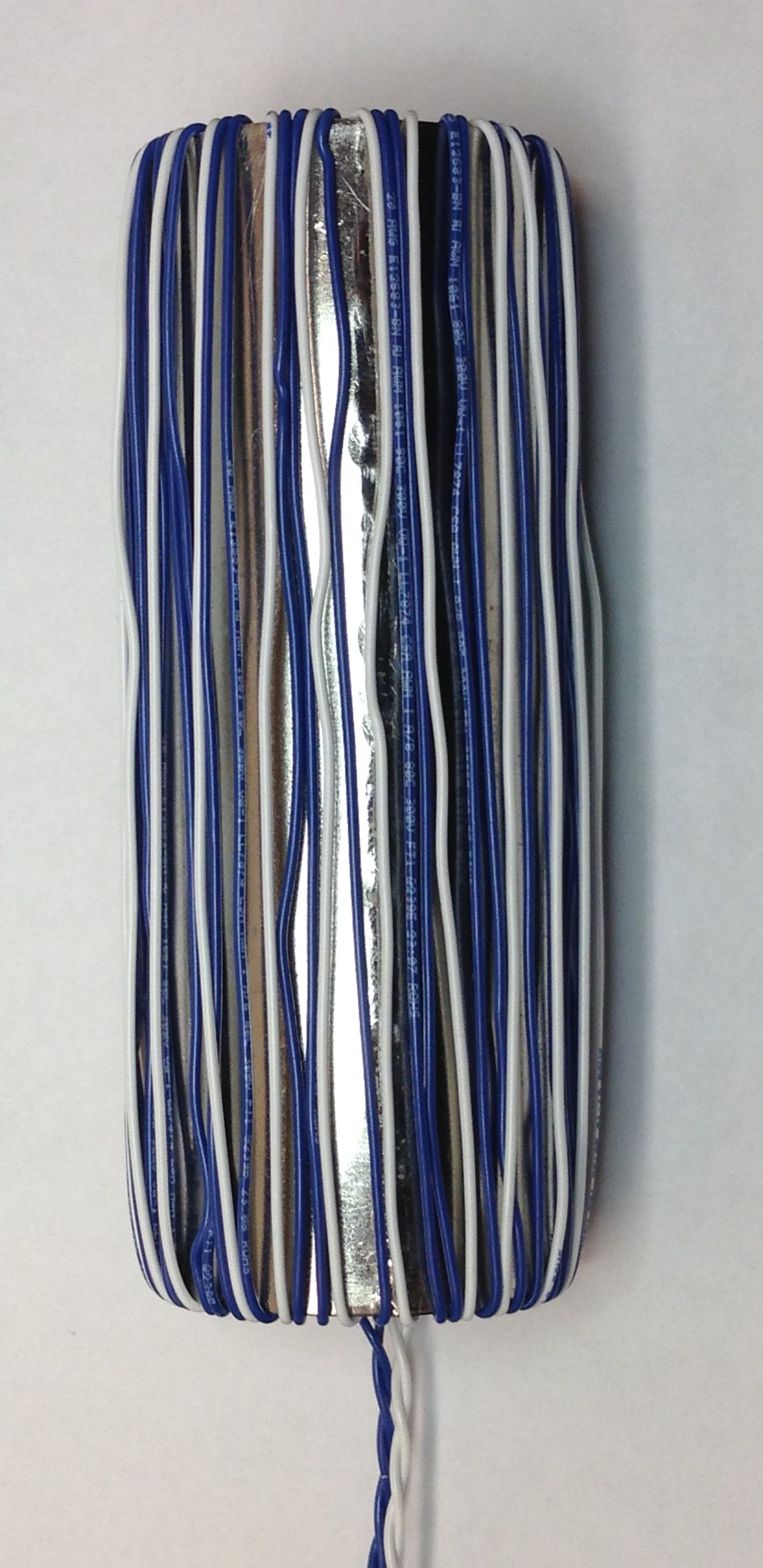
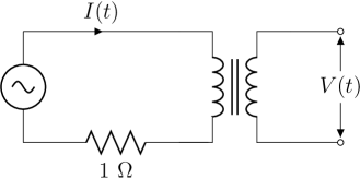
Figure 4: Photograph of a witness cylinder showing transformer windings (left) and schematic of the transformer measurement (right). The primary coil was driven by the sine-out of an SR830 lock-in amplifier, which was also used to demodulate induced voltage $V(t)$ in the secondary coil. The driving current $I(t)$ was sensed by measuring the voltage across a stable 1 $\Omega$ resistor.

The primary coil generated an AC magnetic field as a function of time $H(t)$, while the secondary coil was used to measure the emf induced by the time-varying magnetic flux proportional to $dB(t)/dt$. To a good approximation

$$H_{m}(t)=\frac{N_{p}I(t)}{2\pi R}$$ (4)

where $N_{p}$ is the number of turns in the primary, $I(t)$ is the current in the primary, and $R$ is the radius of the witness cylinder, and

$$\frac{dB_{m}(t)}{dt}=\dot{B}_{m}(t)=\frac{V(t)}{b\ell}$$ (5)

where $V(t)$ is the voltage generated in the secondary, and $b$ and $\ell$ are the thickness and length of the witness cylinder respectively. For a sinusoidal drive current $I(t)$, and under the assumption that $B_{m}(t)=\mu H_{m}(t)$ with $\mu$ being a constant, the voltage generated in the secondary $V(t)$ should be sinusoidal and out of phase with the primary current.

The internal oscillator of an SR830 lock-in amplifier was used to generate $I(t)$. This was monitored by measuring the voltage across a 1 $\Omega$ resistor with small temperature coefficient in the primary loop. The lock-in amplifier was then used to demodulate $V(t)$ into its in-phase $V_{X}$ and out-of-phase $V_{Y}$ components (or equivalently $\dot{B}_{m}(t)$ being demodulated into $\dot{B}_{m,X}$ and $\dot{B}_{m,Y}$, as in equation (5)). The experiment was done at 1 Hz with $H_{m}(t)$ as small as possible, typically 0.1 A/m in amplitude, to measure the slope of the minor $B_{m}-H_{m}$ loops near the origin of the $B_{m}-H_{m}$ space.

The temperature of the core was measured continuously using the same thermocouple arrangement described previously. Measurements of $V_{Y}$ as a function of temperature would then signify a change in $\mu$ with temperature. In general, we used ambient temperature variations for the measurements, similar to the procedure used for our axial shielding factor measurements.

The naive expectation is that the out-of-phase $V_{Y}$ component should signify a non-zero $\mu$, and the in-phase $V_{X}$ component should be zero. In practice, due to a combination of saturation, hysteresis, eddy-current losses, and skin-depth effects, the $V_{X}$ component is nonzero. It was found experimentally that keeping the amplitude of $H_{m}(t)$ small compared to the apparent coercivity ($\sim 3$ A/m for the 0.16 cm thick material at 1 Hz frequencies) ensured that the $V_{Y}$ component was larger than the $V_{X}$ component. This is displayed graphically in Fig. 5, where the dependence of $\dot{B}_{m,Y}$ and $\dot{B}_{m,X}$ on the amplitude of the applied $H_{m}(t)$ is displayed, for a driving frequency of 1 Hz. Clearly the value of $\dot{B}_{m,X}$ can be considerable compared to $\dot{B}_{m,Y}$, for larger $H_{m}$ amplitudes near the coercivity. At larger amplitudes, the material goes into saturation. Both $\dot{B}_{m,Y}$ and $\dot{B}_{m,X}$ eventually decrease as expected at amplitudes much greater than the coercivity.

To understand the behavior in Fig. 5, a theoretical model of the hysteresis based on the work of Jiles [37] was used. The model contains a number of adjustable parameters. We adjusted the parameters based on our measurements of $B_{m}-H_{m}$ loops including the initial magnetization curve. These measurements were performed separately from our lock-in amplifier measurements, using an arbitrary function generator and a digital oscilloscope to acquire them. The measurements were done at frequencies from 0.01 to 10 Hz. It was found that the frequency dependence predicted by Ref. [37] gave relatively good agreement with the measured $B_{m}-H_{m}$ loops once the five original (Jiles-Atherton [38]) parameters were tuned.

For the parameters of the (static) Jiles-Atherton model, we used $B_{s}=0.45$ T, $a=3.75$ A/m, $k=2.4$ A/m, $\alpha=2\times 10^{-6}$, $c=0.05$, which were tuned to our $B_{m}-H_{m}$ curve measurements. For classical losses, we used the parameters $\rho=5.7\times 10^{-7}~{}\Omega\cdot$m, $d=1.6$ mm (the thickness of the material), and $\beta=6$ (geometry factor). These parameters were not tuned, but taken from data. For anomalous losses we used the parameters $w=0.005$ m and $H_{0}=0.0075$ A/m, which we also did not tune, instead relying on the tuning performed in Ref. [37].

These parameters were then used to model the measurement presented in Fig. 5, including the lock-in amplifier function. As shown in Fig. 5, trends in the measurements and simulations are fairly consistent. The sign of $\dot{B}_{m,X}$ relative to $\dot{B}_{m,Y}$ is also correctly predicted by the model (we have adjusted them both to be positive, for graphing purposes). We expect that with further tuning of the model, even better agreement could be achieved.

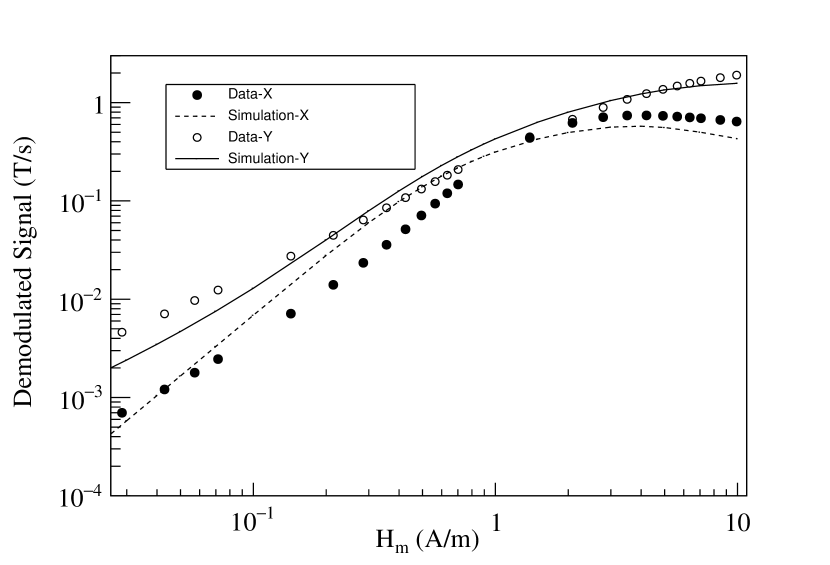
Figure 5: $\dot{B}_{m,X}$ and $\dot{B}_{m,Y}$ as a function of amplitude of the applied $H_{m}$ field at 1 Hz. Points show the acquired data. Curves display the simulation based on the model described in the text.

The model of Ref. [37] makes no prediction of the temperature dependence of the parameters. Ideally, the temperature dependence of $\dot{B}_{m,Y}$ and $\dot{B}_{m,X}$ under various conditions could be used to map out the temperature dependence of the parameters. However, this is beyond the scope of the present work.

We make the simplifying assumption that temperature dependence of $\dot{B}_{m,Y}$ may be approximately interpreted as the temperature dependence of a single parameter $\mu$, i.e. that

$$\frac{1}{\dot{B}_{m,Y}}\frac{d\dot{B}_{m,Y}}{dT}=\frac{1}{\mu}\frac{d\mu}{dT}.$$ (6)

This is justified in part by our selection of measurement parameters (the amplitude of $H_{m}=0.1$ A/m and a measurement frequency of 1 Hz) which ensure that $\dot{B}_{m,Y}$ dominates over $\dot{B}_{m,X}$.

We assign no additional systematic error for this simplification, and all our results are subject to this caveat. We comment further that in our measurements of the axial shielding factor (presented in Section 3.2), the same caveat exists. In that case the in-phase component dominates the demodulated fluxgate signal. In a sense, measuring $\mu(T)$ itself is always an approximation, because it is actually the parameters of minor loops in a hysteresis curve which are measured. In reality, our results may be interpreted as a measure of the temperature-dependence of the slopes of minor loops driven by the stated $H_{m}$.

Measurements of $\frac{1}{\dot{B}_{m,Y}}\frac{d\dot{B}_{m,Y}}{dT}$ as a function of $T$ were made. In general, the data mimicked the behavior of the axial shielding factor measurements, giving a similar level of linearity with temperature as the data displayed in Fig. 3. Other similar behaviors to those measurements were also observed, for example: (a) when the temperature slope changed sign, $\dot{B}_{m,Y}$ would temporarily give a different slope with temperature, (b) the measured value of $\frac{1}{\dot{B}_{m,Y}}\frac{d\dot{B}_{m,Y}}{dT}$ depended on a variety of factors, most notably a dependence on which of the three witness cylinders was used for the measurement, and on differences between subsequent measurements using the same cylinder.

Trial	$\frac{1}{\dot{B}_{m,Y}}\frac{d\dot{B}_{m,Y}}{dT}$	core
#	(%/K)	used
1	0.15	$\alpha$
2	0.03	$\alpha$
3	0.04	$\alpha$
4	0.06	$\alpha$
5	1.07	$\beta$
6	0.93	$\beta$
7	0.88	$\beta$
8	0.88	$\beta$
9	0.09	$\alpha$
10	1.23	$\beta$
11	2.15	$\beta$
12	1.85	$\beta$
13	1.20	$\beta$
14	0.77	$\gamma$

Table 3: Summary of data acquired for the transformer core measurements. Three different witness cylinders, arbitrarily labeled $\alpha$, $\beta$, and $\gamma$, were used for the measurements. A 1 Hz excitation frequency was used with amplitudes for $H_{m}$ ranging from 0.1 to 0.3 A/m. Fluctuations in the temperature ranged from 21-24^∘C and measurement times over a 10-80 hour period are included. Other data acquired for systematic studies are not included in the table.

Table 3 summarizes our measurements of the relative slope $\frac{1}{\dot{B}_{m,Y}}\frac{d\dot{B}_{m,Y}}{dT}$ for a variety of trials, witness cylinders, and numbers of windings. The data show a full range of $0.03-2.15$%/K for $\frac{1}{\mu}\frac{d\mu}{dT}=\frac{1}{\dot{B}_{m,Y}}\frac{d\dot{B}_{m,Y}}{dT}$, again naively assuming the material to be linear as discussed above. The sign of the slope of $\mu(T)$ was the same as the axial shielding factor technique.

A dominant source of variation between results in this method arose from properties inherent to each witness cylinder. One of the cylinders (referred to as $\beta$ in Table 3) gave temperature slopes consistently larger $\frac{1}{\mu}\frac{d\mu}{dT}\sim 0.88-2.15$%/K than the other two $\frac{1}{\mu}\frac{d\mu}{dT}\sim 0.03-0.77$%/K (referred to as $\alpha$ and $\gamma$, with some evidence that $\gamma$ had a larger slope than $\alpha$). We expect this indicates some difference in the annealing process or subsequent treatment of the cylinders, although to our knowledge the treatment was controlled the same as for all three cylinders. Since our goal is to provide input to future EDM experiments on the likely scale of the temperature dependence of $\mu$ that they can expect, we phrase our result as a range covering all these results.

Detailed measurements of the effect of degaussing were conducted for this geometry. The ability to degauss led us ultimately to select a larger number of primary turns (48) so that we could fully saturate the core using only the lock-in amplifier reference output as a current source. A computer program was used to control the lock-in amplifier in order to implement degaussing. A sine wave with the measurement frequency (typically 1 Hz) was applied at the maximum lock-in output power. Over the course of several thousand oscillations, the amplitude was decreased linearly to the measurement amplitude ($\sim 0.1$ A/m). After degaussing with parameters consistent with the recommendations of Refs. [19, 17], the measured temperature slopes were consistent with our previous measurements where no degaussing was done.

Other systematic errors found to contribute at the $<0.1\%$/K level were: motion of the primary and secondary windings, stability of the lock-in amplifier and its current source, and stability of background noise sources.

To summarize, the dominant systematic effects arose due to different similarly prepared cores giving different results, and due to variations in the measured slopes in multiple measurements on the same core. The second of these is essentially the same error encountered in our axial shielding factor measurements. We expect it has the same source; it is possibly a property of the material, or an additional unknown systematic uncertainty.

4 Relationship to nEDM experiments

Neutron EDM experiments are typically designed with the DC coil being magnetically coupled to the innermost magnetic shield. As discussed in Section 2, if the magnetic permeability of the shield changes, this results in a change in the field in the measurement region by an amount $\frac{\mu}{B_{0}}\frac{dB_{0}}{d\mu}=0.01$.

The temperature dependence of $\mu$ has been constrained by two different techniques using open-ended mu-metal witness cylinders annealed at the same time as our prototype magnetic shields. We summarize the overall result as 0.0%/K $<\frac{1}{\mu}\frac{d\mu}{dT}<$ 2.7%/K, where the range is driven in part by material properties of the different mu-metal cylinders, and in part by day-to-day fluctuations in the temperature slopes.

We note the following caveats in relating this measurement to nEDM experiments:

• Although the measurement techniques rely on considerably larger frequencies and different $H_{m}$-fields than those relevant to typical nEDM experiments, we think it reasonable to assume the temperature dependence of the effective permeability should be of similar scale. For frequency, both techniques typically used a 1 Hz AC field, whereas for nEDM experiments the field is DC and stable at the 0.01 Hz level. Furthermore, in one measurement technique the amplitude of $H_{m}$ was $\sim 0.004$ A/m and in the other was $\sim 0.1$ A/m. For nEDM experiments $H_{m}<0.007$ A/m and is DC.

• Both measurement techniques extract an effective $\mu$ that describes the slope of minor loops in $B_{m}-H_{m}$ space. A more correct treatment would include a more comprehensive accounting of hysteresis in the material, which is beyond the scope of this work.

Assuming our measurement of 0.0%/K $<\frac{1}{\mu}\frac{d\mu}{dT}<2.7$%/K and the generic EDM experiment sensitivity of $\frac{\mu}{B_{0}}\frac{dB_{0}}{d\mu}=0.01$ results in a temperature dependence of the magnetic field in a typical nEDM experiment of $\frac{dB_{0}}{dT}=0-270$ pT/K. To achieve a goal of $\sim 1$ pT stability in the internal field for nEDM experiments, the temperature of the innermost magnetic shield in the nEDM experiment should then be controlled to the $<0.004$ K level if the worst-case dependence is to be taken into account. This represents a potentially challenging design constraint for future nEDM experiments.

As noted by others [39], the use of self-shielded coils to reduce the coupling of the $B_{0}$ coil to the innermost magnetic shield is an attractive option for EDM experiments. The principle of this technique is to have a second coil structure between the inner coil and the shield, such that the net magnetic field generated by the two coils is uniform internally but greatly reduced externally. For a perfect self-shielded coil, the field at the position of the magnetic shield would be zero, resulting in perfect decoupling, which is to say a reaction factor that is identically unity. For ideal geometries, such as spherical coils [40, 41, 42] or infinitely long sine-phi coils [43, 44, 45], the functional form of the inner and outer current distributions are the same, albeit with appropriately scaled magnitudes and opposite sign. More sophisticated analytical and numerical methods have been used extensively in NMR and MRI to design self-shielded gradient [46, 47], shim [48, 49], and transmit coils [45, 50], and should be of value in the context of nEDM experiments, as well. We are also pursuing novel techniques for the design of self-shielded coils of any arbitrary field profile and geometric shape [51].

5 Conclusion

In the axial shielding factor measurement, we found 0.6%/K $<\frac{1}{\mu}\frac{d\mu}{dT}<2.7\%$/K, with the measurement being conducted with a typical $H_{m}$-amplitude of 0.004 A/m and at a frequency of 1 Hz. In the transformer core case, we found 0.0%/K $<\frac{1}{\mu}\frac{d\mu}{dT}<2.2\%$/K, with the measurement being conducted with a typical $H_{m}$-amplitude of 0.1 A/m and at a frequency of 1 Hz.

The primary caveat to these measurements is that both measurements (transformer core and axial shielding factor) do not truly measure $\mu$. Rather they measure observables related to the slope of minor hysteresis loops in $B_{m}-H_{m}$ space. They would be more appropriately described by a hysteresis model like that of Jiles [37], but to extract the temperature dependence of all the parameters of the model is beyond the scope of this work. Instead we acknowledge this fact and relate the temperature dependence of the effective $\mu$ measured by each experiment.

We think it is interesting and useful information that the two experiments measure the same scale and sign of the temperature dependence of their respective effective $\mu$’s. This is a principal contribution of this work.

In future work, we plan to measure $B_{0}(T)$ directly for nEDM-like geometries using precision atomic magnetometers. We anticipate based on the present work that self-shielded coil geometries will achieve the best time and temperature stability.

6 Acknowledgments

We thank D. Ostapchuk from The University of Winnipeg for technical support. We gratefully acknowledge the support of the Natural Sciences and Engineering Research Council Canada, the Canada Foundation for Innovation, and the Canada Research Chairs program.

References

References

- [1] A. P. Serebrov et al., JETP Lett. 99, 4 (2014).
- [2] A. P. Serebrov et al., Phys. Procedia 17, 251 (2011).
- [3] K. Kirch, AIP Conf. Proc. 1560, 90 (2013).
- [4] C. A. Baker, et al., Phys. Procedia 17, 159 (2011).
- [5] I. Altarev, et al., Nuovo Cim. C 35, 122 (2012).
- [6] R. Golub and S. K. Lamoreaux, Phys. Rept. 237, 1 (1994).
- [7] T. M. Ito (for the nEDM Collaboration), J. Phys. Conf. Ser. 69 012037, 2007.
- [8] R. Picker (for the TRIUMF Japan-Canada UCN Collaboration), in the proceedings of MENU2016, July 25-30, 2016, Kyoto, Japan, arXiv:1612.00875 [physics.ins-det].
- [9] C. A. Baker, et al., Phys. Rev. Lett. 97, 131801 (2006).
- [10] J. M. Pendlebury et al., Phys. Rev. D 92, 092003 (2015).
- [11] T. Bryś, et al., Nucl. Instrum. Meth. A 554, 527 (2005).
- [12] S. Afach, et al., J. Appl. Phys. 116, 084510 (2014).
- [13] I. Altarev, et al. Rev. Sci. Instrum. 85, 075106 (2014).
- [14] M. Sturm, Masterarbeit, T.U. München (2013).
- [15] B. Patton, E. Zhivun, D. C. Hovde, and D. Budker, Phys. Rev. Lett. 113, 013001 (2014).
- [16] I. Altarev et al., Rev. Sci. Instrum. 85, 075106 (2014).
- [17] I. Altarev et al., J. Appl. Phys. 117, 233903 (2015).
- [18] J. Voigt et al., Metrol. Meas. Syst. 20, 239 (2013).
- [19] F. Thiel et al., Rev. Sci. Instrum. 78, 035106 (2007).
- [20] Z. Sun et al., J. Appl. Phys. 119, 193902 (2016).
- [21] B. Franke, PhD Thesis, ETH Zürich (2013).
- [22] G. Couderchon, J. F. Tiers, J. Magn. Magn. Mat. 26, 196 (1982).
- [23] Krupp VDM Magnifer 7904, Material Data Sheet No. 9004, Aug. 2000, Krupp VDM GmbH, Postfach 18 20, D-58778 Werdohl, Germany.
- [24] K. Gupta, K. K. Raina, S. K. Sinha, J. Alloys Compd. 429, 357 (2007).
- [25] R. M. Bozorth, Ferromagnetism (IEEE Press, Piscataway, NJ, 1993).
- [26] C. P. Bidinosti, J. W. Martin, AIP Advances 4, 047135 (2014).
- [27] L. Urankar, R. Oppelt, IEEE Trans. Biomed. Eng. 43, 697 (1996).
- [28] A. Knecht, PhD Thesis, U. Zürich (2009).
- [29] Finite Element Method Magnetics FEMM version 4.2, available from http://www.femm.info.
- [30] R.H. Lambert and C. Uphoff, Rev. Sci. Instrum. 46, 337 (1975).
- [31] T.J. Sumner, J. Phys. D: Appl. Phys. 20 692 (1987).
- [32] F. Pfeifer and C. Radeloff, J. Magn. Magn. Mat. 19, 190 (1980).
- [33] J. W. Martin et al., Nucl. Instrum. Meth. A 778, 61 (2015).
- [34] Bartington Instruments Ltd., 10 Thorney Leys Business Park, Witney, Oxon, OX28 4GG, England.
- [35] Stanford Research Systems, 1290-D Reamwood Ave., Sunnyvale, CA 94089.
- [36] E. Paperno, IEEE Trans. Magn. 35, 3940 (1999).
- [37] D. C. Jiles, J. Appl. Phys. 76, 5849 (1994).
- [38] D. C. Jiles and D. L. Atherton, J. Appl. Phys. 55, 2115 (1984); D. C. Jiles and D. L. Atherton, J. Magn. Magn. Mat. 61, 48 (1986).
- [39] I. B. Khriplovich, S. Lamoreaux, CP violation without strangeness: electric dipole moments of particles, atoms, and molecules. (Springer-Verlag, Berlin, 2012).
- [40] W. F. Brown Jr. and J. H. Sweer, Rev. Sci. Instrum. 16, 276 (1945).
- [41] H. A. Wheeler, Proceedings of the IRE 46,1595 (1958).
- [42] E.M. Purcell, Am. J. Phys. 57, 18 (1989); Am. J. Phys. 58, 296 (1990).
- [43] R.A. Beth, Brookhaven National Laboratory Report BNL-10143 (1966).
- [44] R.A. Beth, US Patent 3466499, September 9, 1969.
- [45] C.P. Bidinosti, I.S. Kravchuk, and M.E. Hayden, J. Magn. Res. 177, 31 (2005).
- [46] R. Turner and R.M. Bowley, J. Phys. E: Sci. Instrum. 19, 876 (1986).
- [47] S.S. Hidalgo-Tobon, Concepts Magn. Reson. 36A, 223 (2010).
- [48] M.A. Brideson, L.K. Forbes, S. Crozier, Concepts Magn. Reson. 14, 9 (2002).
- [49] L.K. Forbes and S. Crozier, J. Phys. D: Appl. Phys 36, 68 (2003).
- [50] V.V. Kuzmin et al., J. Magn. Reson. 256, 70 (2015).
- [51] C. Crawford, private communication.