Entropically Damped Artificial Compressibility for SPH

Abstract

In this paper, the Entropically Damped Artificial Compressibility (EDAC) formulation of Clausen (2013) is used in the context of the Smoothed Particle Hydrodynamics (SPH) method for the simulation of incompressible fluids. Traditionally, weakly-compressible SPH (WCSPH) formulations have employed artificial compressiblity to simulate incompressible fluids. EDAC is an alternative to the artificial compressiblity scheme wherein a pressure evolution equation is solved in lieu of coupling the fluid density to the pressure by an equation of state. The method is explicit and is easy to incorporate into existing SPH solvers using the WCSPH formulation. This is demonstrated by coupling the EDAC scheme with the recently proposed Transport Velocity Formulation (TVF) of Adami et al. (2013). The method works for both internal flows and for flows with a free surface. Several benchmark problems are considered to evaluate the proposed scheme and it is found that the EDAC scheme gives results that are as good or sometimes better than those produced by the TVF or standard WCSPH. The scheme is robust and produces smooth pressure distributions and does not require the use of an artificial viscosity in the momentum equation although using some artificial viscosity is beneficial.

1 Introduction

The Smoothed Particle Hydrodynamics (SPH) technique was initially developed for astrophysical problems independently by Lucy [1], and Gingold and Monaghan [2]. The method is mesh-free and self-adaptive. With the introduction of the weakly-compressible SPH scheme (WCSPH) by Monaghan [3], the SPH method has been extensively applied to incompressible fluid flow and free-surface problems (see [4] and [5] for a recent review with an emphasis on the application of SPH to industrial fluid flow problems). Alternative to the WCSPH approach, truly incompressible implicit SPH schemes like the projection-SPH [6] and incompressible-SPH [7, 8] have been introduced. These methods satisfy the incompressiblity constraint ($\nabla\cdot\mathbf{u}=0$) by solving a pressure-Poisson equation. The methods differ in how the pressure-Poisson equation is setup. While these schemes are generally considered to be more accurate, the implicit nature of these schemes makes it difficult to implement and parallelize which has lead to the WCSPH approach garnering favor within the SPH community. The Implicit Incompressible SPH scheme (IISPH) [9] proposes an iterative solution procedure to alleviate some of these issues. Recently, an Artificial Compressibility-based Incompressible SPH (ACISPH) scheme [10] has been proposed which applies a traditional dual-time stepping approach used in Eulerian schemes to satisfy incompressibility. This scheme is also explicit and seems a promising alternative to the traditional ISPH schemes.

The weakly-compressible formulation relies on a stiff equation of state that generates large pressure changes for small density variations. A consequence is that the large pressure oscillations need to be damped out, which necessitate the use of some form of artificial viscosity. Another problem with the WCSPH formulation is the appearance of void regions and particle clumping, especially where the pressure is negative. This has resulted in some researchers using problem-specific background pressure values to mitigate this problem. The Transport Velocity Formulation (TVF) of Adami et al. [11] ameliorates some of the above issues by ensuring a more homogeneous distribution of particles by introducing a background pressure field. This background pressure is not tuned to any particular problem. In addition, the particles are moved using an advection (transport) velocity instead of the actual velocity. The advection velocity differs from the momentum velocity through the addition of the constant background pressure. The motion induced by the background pressure is corrected by introducing an additional stress term in the momentum equation. The stiffness of the state equation is reduced by using a value of $\gamma=1$ in the equation of state in contrast to the traditionally chosen value of $\gamma=7$. The scheme produces excellent results for internal flows and virtually eliminates particle clumping and void regions. The scheme also displays reduced pressure oscillations. Recently, the scheme has been extended to handle free-surface flows [12].

The Entropically Damped Artificially Compressible (EDAC) method of Clausen [13, 14] is an alternative to the artificial compressibility used by the weakly-compressible formulation. This method is similar to the kinetically reduced local Navier-Stokes method presented in [15, 16, 17]. However, the EDAC scheme uses the pressure instead of the grand potential as the thermodynamic variable and this simplifies the resulting equations. The EDAC scheme does not rely on an equation of state that relates pressure to density. Instead, an evolution equation for the pressure is derived based on thermodynamic considerations. The fluid is assumed to be isentropic and minimization of density fluctuations leads to an equation for the pressure. This equation includes a damping term for the pressure which reduces pressure oscillations significantly. The scheme in its original form does not introduce any new parameters into the simulation. There is also no need to introduce an artificial viscosity in the momentum equation. It is important to note that the EDAC method is based on artificial compressibility and therefore does require the use of an artificial speed of sound. The method does therefore have similar time step restrictions as the WCSPH scheme. The EDAC method was validated for finite-difference [13] and finite-element [14] schemes and exhibited good parallel performance owing to the elimination of the elliptic pressure Poisson equation. Recently, Delorme et al. [18] have successfully used the EDAC scheme in a high-order finite-difference solver with explicit sub-grid-scale (SGS) terms for Large-Eddy-Simulation (LES).

In this work, the EDAC method is applied to SPH for the simulation of incompressible fluids for both internal and free-surface problems. The motivation for this work arose from the encouraging results (despite a relatively naive implementation) presented in [19]. In that work, it was found that a simple application of the EDAC scheme produced results that were better than the standard WCSPH, though not better than those of the TVF scheme. Upon further investigation, it was found that when the background pressure used in the TVF formulation is set to zero, the EDAC scheme outperforms it. This is because the EDAC scheme provides a smoother pressure distribution than that which is obtained via the equation of state. There is no mechanism within the EDAC framework to ensure a uniform distribution of particles. Therefore, we adapted the TVF scheme to be used along with EDAC. The resulting scheme produces very good results and outperforms the standard TVF for many of the benchmark problems considered in this work.

The proposed EDAC scheme thus comes in two flavors. For internal flows, a formulation based on the TVF is employed where a background pressure is added. This background pressure ensures a homogeneous particle distribution. For free-surface flows, a straight-forward formulation is used with the EDAC to produce very good results. The scheme thus works well for both internal and external flows. Several results are presented along with suitable comparisons between the TVF and standard SPH schemes to demonstrate the new scheme. All the results presented in this work are reproducible through the publicly available PySPH package [20, 21] along with the code in http://gitlab.com/prabhu/edac_sph.

We note that the new scheme proposed is similar to the $\delta$-SPH formulation of Antuono et al. [22] and Marrone et al. [23]. The $\delta$-SPH scheme adds a dissipation term to the continuity equation and uses a linearized equation of state. The resulting scheme is very similar to the EDAC scheme. However, the details of the implementation and origins of the scheme are different. In addition, the present work uses the TVF formulation making the new scheme considerably different in its final form.

The paper is organized as follows. In Section 2, the governing equations for the EDAC scheme are outlined. In Section 3, the SPH discretization for the EDAC equations are presented. In Section 4, the new scheme is evaluated against a suite benchmark problems. The results are compared to the analytical solution where available, and to the traditional WCSPH and TVF formulations wherever possible. In Section 5, the paper is concluded with a summary.

2 The EDAC method

The EDAC method is discussed in detail in [13, 14]. In this method, the density of the fluid $\rho$ is held fixed and an evolution equation for the pressure based on thermodynamic considerations is derived. As a result, a pressure evolution equation needs to be solved in addition to the momentum equation. The equations are,

$$\frac{d\mathbf{u}}{dt} =-\frac{1}{\rho}\nabla p+\text{div}(\mathbf{\sigma}),$$ (1)

$$\frac{dp}{dt} =-\rho c_{s}^{2}\text{div}(\mathbf{u})+\nu\nabla^{2}p,$$ (2)

where $\mathbf{u}$ is the velocity of the fluid, $p$ is the pressure, $\sigma$ is the deviatoric part of the stress tensor, $c_{s}$ is the speed of sound, and $\nu$ is the kinematic viscosity of the fluid.

As is typically chosen in WCSPH schemes, the speed of sound is set to a multiple of the maximum fluid velocity. In this paper $c_{s}=10\ u_{\max}$ unless otherwise mentioned.

In this work, the fluid is assumed to be Newtonian, which results in the following momentum equation:

$$\frac{d\mathbf{u}}{dt} =-\frac{1}{\rho}\nabla p+\nu\nabla^{2}\mathbf{u}.$$ (3)

On comparison of the EDAC method with the standard WCSPH formulation, it can be seen that the momentum equation is unchanged and equation (2) replaces the continuity equation, $\frac{d\rho}{dt}=-\rho\ \text{div}(\mathbf{u})$. Also, owing to the pressure evolution equation in EDAC, there is no need for an equation of state to couple the fluid density and pressure.

The EDAC equation (2), is derived in [13]. Two simplifying assumptions are made in this derivation. The first is to ignore the viscous dissipation term, $\phi$. The second is to set the Prandtl number $Pr=\gamma$. The first assumption is also made in the case of the traditional artificial compressibility schemes (as can be seen in equation 7 of Clausen [13]). Clausen [13] shows that the artificial compressibility equation results when isentropic flow is assumed and this implies that the fluid is inviscid and therefore the viscous dissipation is ignored. For the EDAC equation, instead of assuming isentropy, one drives the density fluctuations to zero resulting in a different thermodynamic relationship. The viscous dissipation is neglected to simplify the resulting equations. What is crucial in the EDAC equation is the second derivative of pressure which smoothes the pressure through the introduction of entropy. The second assumption to set $Pr=\gamma$ is arbitrary and in the numerical simulations for the current work, a numerical viscosity value is found to be more well suited (see section 3.3).

In summary, the EDAC scheme essentially introduces entropy by damping the pressure oscillations. It is to be noted that this is the only difference from the WCSPH. As mentioned in the introduction, a similar approach is used in [22, 23], where a damping term is introduced in the continuity equation. With the EDAC scheme, the pressure is evolved directly rather than computed from the density. It is important to note that the introduction of pressure damping is not directly equivalent to adding an artificial viscosity to the momentum equation as the pressure only affects the momentum equation via its gradient. The approach is similar to the density filtering approach (see [24] for more details). However, the pressure field is smoothed at every step in the present case and not after every $m$ steps.

In the next section, an SPH-discretization of these equations is performed to obtain the numerical scheme.

3 Numerical implementation

As discussed in the introduction, there are two major issues that arise when using weakly-compressible SPH (WCSPH) formulations. The first is the presence of large pressure oscillations due to the stiff equation of state and the second is due to the inhomogeneous particle distributions. The basic EDAC formulation solves the first problem [19]. The TVF scheme solves the second problem by the introduction of a background pressure for internal flows. Based on this, two different formulations using the EDAC are presented in the following. The first formulation is what is called the standard EDAC formulation. This formulation can be used for external flows. The second formulation is what is called the EDAC TVF formulation, which is based on the TVF formulation and can be applied to internal flows where it is possible to use a background pressure. Numerical discretizations for both these schemes are discussed next.

3.1 The standard EDAC formulation

The EDAC formulation keeps the density constant and this eliminates the need for the continuity equation or the use of a summation density to find the pressure. However, in SPH discretizations, $m/\rho$ is typically used as a proxy for the particle volume. The density of the fluids can therefore be computed using the summation density approach. This density does not directly affect the pressure as there is no equation of state. In the case of solid walls, the density of any wall particle is set to a constant. The classic summation density equation for SPH is recalled:

$$\rho_{i}=\sum_{j}m_{j}W_{ij},$$ (4)

where $W_{ij}=W(|\mathbf{r_{i}}-\mathbf{r_{j}}|,h)$ is the kernel function chosen for the SPH discretization and $h$ is the kernel radius parameter. In this paper, the quintic spline kernel is used, which is given by,

$$W(q)=\left\{\begin{array}[]{ll}\alpha_{2}\left[{(3-q)}^{5}-6{(2-q)}^{5}+15{(1-q)}^{5}\right],&\textrm{for}\ 0\leq q\leq 1,\\ \alpha_{2}\left[{(3-q)}^{5}-6{(2-q)}^{5}\right],&\textrm{for}\ 1<q\leq 2,\\ \alpha_{2}\ {(3-q)}^{5},&\textrm{for}\ 2<q\leq 3,\\ 0,&\textrm{for}\ q>3,\\ \end{array}\right.$$ (5)

where $\alpha_{2}=7/(478\pi h^{2})$ in two-dimensions, and $q=|\mathbf{r}|/h$.

In the previous work [19], Monaghan’s original formulation was used for the pressure gradient and the formulation due to Morris et al. [25] was used for the viscous term in equation (3). The method of Adami et al. [26] was used to implement the effect of boundaries.

In the present work, a number density based formulation is employed as used in [26], which results in the following momentum equation:

$$\frac{d\mathbf{u}_{i}}{dt}=\frac{1}{m_{i}}\sum_{j}\left(V_{i}^{2}+V_{j}^{2}\right)\left[-\tilde{p}_{ij}\nabla W_{ij}+\tilde{\eta}_{ij}\frac{\mathbf{u}_{ij}}{(r_{ij}^{2}+\eta h_{ij}^{2})}\nabla W_{ij}\cdot\mathbf{r}_{ij}\right]+\mathbf{g}_{i},$$ (6)

where $\mathbf{r}_{ij}=\mathbf{r}_{i}-\mathbf{r}_{j}$, $\mathbf{u}_{ij}=\mathbf{u}_{i}-\mathbf{u}_{j}$, $h_{ij}=(h_{i}+h_{j})/2$, $\eta=0.01$,

$$V_{i}=\frac{1}{\sum_{j}W_{ij}},$$ (7)

$$\tilde{p}_{ij}=\frac{\rho_{j}p_{i}+\rho_{i}p_{j}}{\rho_{i}+\rho_{j}},$$ (8)

$$\tilde{\eta}_{ij}=\frac{2\eta_{i}\eta_{j}}{\eta_{i}+\eta_{j}},$$ (9)

where $\eta_{i}=\rho_{i}\nu_{i}$.

The EDAC pressure evolution equation (2) is discretized using a similar approach to the momentum equation to be,

$$\frac{dp_{i}}{dt} =\sum_{j}\frac{m_{j}\rho_{i}}{\rho_{j}}c_{s}^{2}\ \mathbf{u_{ij}}\cdot\nabla W_{ij}+\frac{(V_{i}^{2}+V_{j}^{2})}{m_{i}}\tilde{\eta}_{ij}\frac{p_{ij}}{(r_{ij}^{2}+\eta h_{ij}^{2})}\nabla W_{ij}\cdot\mathbf{r}_{ij},$$ (10)

where $p_{ij}=p_{i}-p_{j}$. The particles are moved according to,

$$\frac{d\mathbf{r}_{i}}{dt}=\mathbf{u}_{i}.$$ (11)

Upon the specification of suitable initial conditions for $\mathbf{u}$, $p$, $m$, and $\mathbf{r}$, equations (4), (6), (10), and (11) are sufficient for simulating the flow in the absence of any boundaries.

3.2 EDAC TVF formulation

In WCSPH, as the particles move they tend to become disordered. This introduces significant errors in the simulation. The particle positions can be regularized by the addition of a background pressure. A naive approach would be to simply add a constant pressure and use it in the governing equations. However, as shown by Basa et al. [27], the error in computing the gradient of pressure increases when the pressure values are large. They subtract the average pressure to reduce this error. The TVF scheme of Adami et al. [11] overcomes this by advecting the particles using an arbitrary background pressure through the “transport velocity” and correct for this background pressure using an additional stress term in the momentum equation. This ensures a homogeneous particle distribution without introducing a constant background pressure in the pressure derivative term.

For internal flows, the TVF formulation is adapted to introduce the background pressure. The density is computed using the summation density equation (4). As before, this is mainly to serve as a proxy for the particle volume in the SPH discretizations. The momentum equation for the TVF scheme as discussed in Adami et al. [11] is given by,

$$\begin{split}\frac{\tilde{d}\mathbf{u}_{i}}{dt}=\frac{1}{m_{i}}\sum_{j}\left(V_{i}^{2}+V_{j}^{2}\right)&\left[-\tilde{p}_{ij}\nabla W_{ij}+\frac{1}{2}(\mathbf{A}_{i}+\mathbf{A}_{j})\cdot\nabla W_{ij}\right.\\ &\left.+\tilde{\eta}_{ij}\frac{\mathbf{u}_{ij}}{(r_{ij}^{2}+\eta h_{ij}^{2})}\nabla W_{ij}\cdot\mathbf{r}_{ij}\right]+\mathbf{g}_{i},\end{split}$$ (12)

where $\mathbf{A}=\rho\mathbf{u}(\mathbf{\tilde{u}}-\mathbf{u})$, $\mathbf{\tilde{u}}$ is the advection or transport velocity and the material derivative, $\frac{\tilde{d}}{dt}$ is given as,

$$\frac{\tilde{d}(\cdot)}{dt}=\frac{\partial(\cdot)}{\partial t}+\mathbf{\tilde{u}}\cdot\text{grad}(\mathbf{\cdot}).$$ (13)

Thus the particles move using the transport velocity,

$$\frac{d\mathbf{r}_{i}}{dt}=\mathbf{\tilde{u}}_{i}.$$ (14)

The transport velocity is obtained from the momentum velocity $\mathbf{u}$ at each time step using,

$$\mathbf{\tilde{u}}_{i}(t+\delta t)=\mathbf{u}_{i}(t)+\delta t\left(\frac{\tilde{d}\mathbf{u}_{i}}{dt}-\frac{p_{b}}{m_{i}}\sum_{j}\left(V_{i}^{2}+V_{j}^{2}\right)\nabla W_{ij}\right),$$ (15)

where $p_{b}$ is the background pressure.

In the TVF scheme, the pressure is computed from the density using the standard equation of state with a value of $\gamma=1$. Instead, the EDAC equation (10) is used to evolve the pressure. In the present approach, the pressure reduction technique proposed by Basa et al. [27] is used to mitigate the errors due to large pressures. This requires the computation of the average pressure of each particle, $p_{\text{avg}}$:

$$p_{\text{avg},i}=\sum_{j=1}^{N_{i}}\frac{p_{j}}{N_{i}},$$ (16)

where $N_{i}$ are the number of neighbors for the particle $i$ and includes both fluid and boundary neighbors. Equation (8) is then replaced with,

$$\tilde{p}_{ij}=\frac{\rho_{j}(p_{i}-p_{avg,i})+\rho_{i}(p_{j}-p_{avg,i})}{\rho_{i}+\rho_{j}}.$$ (17)

In Section 4 it can be seen that this results in significantly improved results that outperform the traditional TVF scheme. It is worth mentioning that this technique, applied to the standard SPH or to the standard TVF scheme does not result in any significant improvement.

The boundary conditions are satisfied using the formulation of Adami et al. [26]. This method uses fixed wall particles and sets the pressure and velocity of these wall particles in order to accurately simulate the boundary conditions. The same scheme is used here with the only modification being that the density of the boundary particles is not set based on the pressure of the boundary particles (i.e. equation (28) in Adami et al. [26] is not used).

3.3 Suitable choice of $\nu$ for EDAC

In equation (10) one can see that the viscosity $\nu$ is used to diffuse the pressure. The original formulation assumes that the value of $\nu$ is the same as the fluid viscosity. In our numerical experiments it was found that if the viscosity is too small, the pressure builds up too fast and eventually blows up. If the viscosity is too large it diffuses too fast resulting in a non-physical simulation. Thus, the physical viscosity is not always the most appropriate. Instead using,

$$\nu_{edac}=\frac{\alpha hc_{s}}{8},$$ (18)

works very well. The choice of $\nu_{edac}$ is motivated by the expression for artificial viscosity in traditional WCSPH formulations. The form of the viscous term used in [22, 23] is also the same. In this paper, it is found that $\alpha=0.5$ is a good choice for a wide range of Reynolds numbers (0.0125 to 10000). While this choice of $\nu_{edac}$ is motivated by the expression for artificial viscosity traditionally used in the SPH, the viscous damping of pressure is not the same as adding artificial viscosity directly to the momentum equation.

To summarize the schemes,

• for external flow problems, equations (4), (6), and (10) are used. The particles move with the fluid velocity $\mathbf{u}$ and are advected according to (11).

• for internal flows, equations (4), (12), (16), (17) and (10) are used. Equation (14) is used to advect the particles. The transport velocity is found from equation (15).

For each of the schemes, the value of $\nu$ used in the equation (10) is found using equation (18). The value of $\nu$ used in the momentum equation is the fluid viscosity.

The proposed EDAC scheme is explicit and as such, any suitable integrator can be used. In this work, one of the two simplest possible two-stage explicit integrators is chosen. For both integrators, the particle properties are first predicted at $t+\delta t/2$. The right-hand-side (RHS) is subsequently evaluated at this intermediate step and the final properties at $t+\delta t$ are obtained by correcting the predicted values. Two variants of this predictor-corrector integration scheme are defined. In the first type, the prediction stage is completed using the RHS from the previous time-step. This is called the Predict-Evaluate-Correct (PEC) type integrator. In the second variant, an evaluation of the RHS is carried out for the predictor stage. This integrator, deemed Evaluate-Predict-Evaluate-Correct (EPEC) is more accurate (at the cost of two RHS evaluations per time-step). For the standard EDAC scheme the time integration proceeds as follows. The predictor step is first performed as,

$$\mathbf{u}^{n+\frac{1}{2}} =\mathbf{u}^{n}+\frac{\Delta t}{2m}\mathbf{f}^{n-\frac{1}{2}}$$ (19)

$$\mathbf{r}^{n+\frac{1}{2}} =\mathbf{r}^{n}+\frac{\Delta t}{2}\mathbf{u}^{n-\frac{1}{2}}$$

$$p^{n+\frac{1}{2}} =p^{n}+\frac{\Delta t}{2}\ a_{p}^{n-\frac{1}{2}},$$

where $a_{p}$ is the right hand side of equation (10). The new accelerations are then computed at this point and the corrector step is as,

$$\mathbf{u}^{n+1} =\mathbf{u}^{n}+\frac{\Delta t}{m}\ \mathbf{f}^{n+\frac{1}{2}}$$ (20)

$$\mathbf{r}^{n+1} =\mathbf{r}^{n}+\frac{\Delta t}{m}\ \mathbf{u}^{n+\frac{1}{2}}$$

$$p^{n+1} =p^{n}+\Delta t\ a_{p}^{n+\frac{1}{2}}.$$

For the EDAC TVF method, the predictor step is implemented as,

$$\mathbf{u}^{n+\frac{1}{2}} =\mathbf{u}^{n}+\frac{\Delta t}{2m}\ \mathbf{f}^{n-\frac{1}{2}}$$ (21)

$$\mathbf{\tilde{u}}^{n+\frac{1}{2}} =\mathbf{u}^{n+\frac{1}{2}}+\frac{\Delta t}{2m}\ \mathbf{f_{p_{b}}}^{n-\frac{1}{2}}$$

$$\mathbf{r}^{n+\frac{1}{2}} =\mathbf{r}^{n}+\frac{\Delta t}{2}\ \mathbf{\tilde{u}}^{n+\frac{1}{2}}$$

$$p^{n+\frac{1}{2}} =p^{n}+\frac{\Delta t}{2}\ a_{p}^{n-\frac{1}{2}},$$

where $\mathbf{f}_{p_{b}}$ is the background pressure force. At this point the accelerations are computed and the corrector step is performed as,

$$\mathbf{u}^{n+1} =\mathbf{u}^{n}+\frac{\Delta t}{m}\ \mathbf{f}^{n+\frac{1}{2}}$$ (22)

$$\mathbf{\tilde{u}}^{n+1} =\mathbf{u}^{n+1}+\frac{\Delta t}{m}\ \mathbf{f_{p_{b}}}^{n+\frac{1}{2}}$$

$$\mathbf{r}^{n+1} =\mathbf{r}^{n}+\Delta t\ \mathbf{\tilde{u}}^{n+1}$$

$$p^{n+1} =p^{n}+\Delta t\ a_{p}^{n+\frac{1}{2}}.$$

As mentioned in the introduction, all the equations and algorithms presented in this work are implemented using the PySPH framework [20, 21, 28]. PySPH is an open source framework for SPH that is written in Python. It is easy to use, easy to extend, and supports non-intrusive parallelization and dynamic load balancing. PySPH provides an implementation of the TVF formulation and this allows for a comparison of the results with those of the standard SPH and TVF where necessary. In the next section, the performance of the proposed SPH scheme is evaluated for several benchmark problems of varying complexity.

4 Numerical Results

In this section the EDAC scheme is applied to a suite of test problems. The results from the new EDAC scheme are compared with the standard weakly compressible SPH (WCSPH) and, where possible, with those from the Transport-Velocity-Formulation (TVF) scheme [11].

Every attempt has been made to allow easy reproduction of all of the present results. The TVF implementation is available as part of PySPH [28] as is an implementation of EDAC-SPH. Every figure in this article is automatically generated. The approach and tools used for this are described in detail in [29]. The code for the EDAC implementation and the automation of all of our results are available from http://gitlab.com/prabhu/edac_sph.

4.1 Taylor Green Vortex

The Taylor-Green vortex problem is a particularly challenging case to simulate using SPH. This is an exact solution of the Navier-Stokes equations in a periodic domain. Here, a two-dimensional version is considered as is done in [11]. The fluid is considered periodic in both directions and the exact solution is given by,

$$u =-Ue^{bt}\cos(2\pi x)\sin(2\pi y)$$ (23)

$$v =Ue^{bt}\sin(2\pi x)\cos(2\pi y)$$ (24)

$$p =-U^{2}e^{2bt}(\cos(4\pi x)+\cos(4\pi y))/4,$$ (25)

where $U$ is chosen as $1m/s$, $b=-8\pi^{2}/Re$, $Re=UL/\nu$, and $L=1m$.

The Reynolds number, $Re$, is initially chosen to be $100$. The flow is initialized with $u,v,p$ set to the values at $t=0$. The evolution of the quantities are studied for different numerical schemes. The speed of sound is set to $10$ times the maximum flow velocity at $t=0$. The background pressure is set as discussed by Adami et al. [11] to $p_{b}=c_{s}^{2}\rho$. The quintic spline kernel is used with the smoothing length $h$ set to the particle spacing $\Delta x$. The value of $\alpha$ in the equation (18) is chosen as 0.5. The results from the standard SPH scheme, the TVF, and the new scheme are compared. Since a physical viscosity is used and the solution to the problem remains smooth, no artificial viscosity is used for any of the schemes.

A Predict-Evaluate-Correct (PEC) integrator with a fixed time-step is used and chosen as per the following equation,

$$\Delta t=\min\left(\frac{h}{4(c_{s}+|U_{max}|)},\ \frac{h^{2}}{8\nu}\right).$$ (26)

Unless explicitly mentioned, all simulations use this integrator and a time-step chosen as above.

In Adami et al. [11], the simulation starts with either uniformly distributed particles or with a “relaxed initial condition”. For the relaxed initial condition, the authors use the particle distribution generated by the uniformly distributed case at the final time and impose an analytical initial condition at the particle positions. The results for the uniformly distributed particles have about an order of magnitude more error than that of the relaxed initialization. This is because the uniform distribution results in particles being placed along (or near) stagnation streamlines resulting in non-uniform particle distributions.

In this work, for this particular problem, the initial distribution is uniform but a small random displacement is added to the particles. The random displacement is uniformly distributed and the maximum displacement in any coordinate direction is chosen to be $\Delta x/5$. The same initial conditions are used for all schemes. This is simple to implement, resolves the problems with stagnation streamlines, and enables for a fair comparison of all the schemes.

Figure 1: The decay with time of the velocity magnitude for the different schemes. Particles are initialized with $n_{x}=n_{y}=50$ and thereafter randomly perturbed. The Reynold’s number is chosen to be $Re=100$. The quintic spline kernel is used with a smoothing length equal to the initial (undisturbed) particle spacing.

In Fig. 1, the decay of the maximum velocity magnitude produced by different schemes is compared with the exact solution. A regular particle distribution with $n_{x}=n_{y}=50$ is randomly perturbed as discussed above. The standard SPH, TVF, standard EDAC (labeled EDAC ext), and TVF EDAC (labeled EDAC) schemes are compared. As can be seen, the EDAC and TVF perform best. The standard EDAC without the TVF (labeled EDAC ext) is better than the standard SPH but not as effective as the TVF scheme. As discussed in previous sections, this occurs because the TVF background pressure results in a more homogeneous particle distribution.

Fig. 1 does not clearly differentiate between schemes. The $L_{1}$ error of $|\mathbf{u}|$ is a better measure of the performance of the schemes and is plotted in Fig. 2. The $L_{1}$ error is computed as the average value of the difference between the exact velocity magnitude and the computed velocity magnitude, that is,

$$L_{1}=\frac{\sum_{i}|\mathbf{u_{i,computed}}|-|\mathbf{u_{i,exact}}|}{\sum_{i}|\mathbf{u_{i,exact}}|},$$ (27)

where the value of $\mathbf{u}$ is computed at the particle positions for each particle $i$ in the flow.

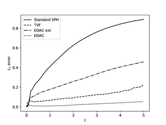
Figure 2: The $L_{1}$ error of the velocity magnitude vs. $t$ for the standard SPH (solid line), standard EDAC (dash-dot), EDAC TVF (dot) and TVF (dash) schemes.

Fig. 2 clearly brings out the differences in the schemes. It is easy to see that the TVF EDAC scheme (labeled EDAC) produces much lower errors than the TVF scheme (by almost a factor of 4). The difference between the standard EDAC scheme and the TVF is also brought out. It is easy to see that the standard EDAC scheme (labeled EDAC ext) is better than the standard SPH.

In order to better understand the behavior of the methods, several other variations of the basic schemes have been studied. Fig. 3 shows the $L_{1}$ error of the velocity magnitude using the TVF formulation, along with the background pressure correction scheme of Basa et al. [27] (labeled as “TVF + BQL”). The results of using the TVF without any background pressure is labeled as “TVF (pb=0)”. This clearly shows that the pressure correction of Basa et al. does not affect the TVF scheme, and that without the background pressure, the standard EDAC is in fact better than the TVF. While this is only to be expected, it does highlight that the EDAC scheme performs very well. The plot labeled “EDAC no-BQL” demonstrates that the pressure correction due to Basa et al. [27] is necessary for the EDAC scheme. It is also found (not shown here) that using the pressure correction with the standard SPH formulation does not produce any significant advantages. Similarly, the tensile correction of Monaghan [30] has no major influence on the results.

Figure 3: The $L_{1}$ error of the velocity magnitude versus $t$ for other variations of the schemes.

The EDAC scheme evolves the pressure in a very different manner from the traditional WCSPH schemes. It is important to see how it captures the pressure field as compared with the other schemes. In Fig. 4, the $L_{1}$ error in the pressure is plotted as the simulation evolves. The pressure in the EDAC scheme drifts due to the use of the transport velocity used to move the particles, we therefore compute $p-p_{avg}$ where $p_{avg}$ is computed using equation (16). In order to make the comparisons uniform this is done for all the schemes. This does not change the quality of the results by much. The error is computed as,

$$p_{L_{1}}=\frac{\sum_{i}|p_{i,computed}-p_{i,avg}-p_{i,exact}|}{\text{max}_{i}(p_{i,exact})}.$$ (28)

As can be clearly seen in Fig. 4, the new EDAC scheme outperforms all other schemes. It should be noted that the magnitude of the error in the pressure is rather large for all schemes suggesting that all of the schemes have difficulty in capturing the pressure field accurately.

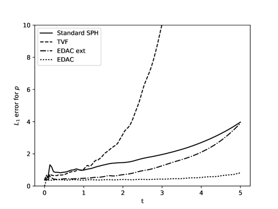
Figure 4: The $L_{1}$ error of the pressure versus $t$ for the Standard SPH (solid line), TVF (dash), EDAC-ext (dash-dot) and EDAC (dot) schemes.

Fig. 5 shows the distribution of particles for the case where $n_{x}=100$ using the EDAC scheme at a time of $t=2.5$. The color indicates the velocity magnitude. As can be seen, the particles are distributed homogeneously and the results are good. Fig. 6(a) shows the distribution of particles with the color indicating the pressure. The pressure plotted is the difference of the local pressure minus the average of the pressure of all particles. Fig. 6(b) shows the same results when obtained using the TVF. The results show clearly that the EDAC scheme performs well and this is consistent with the $L_{1}$ errors of pressure shown in Fig. 4.

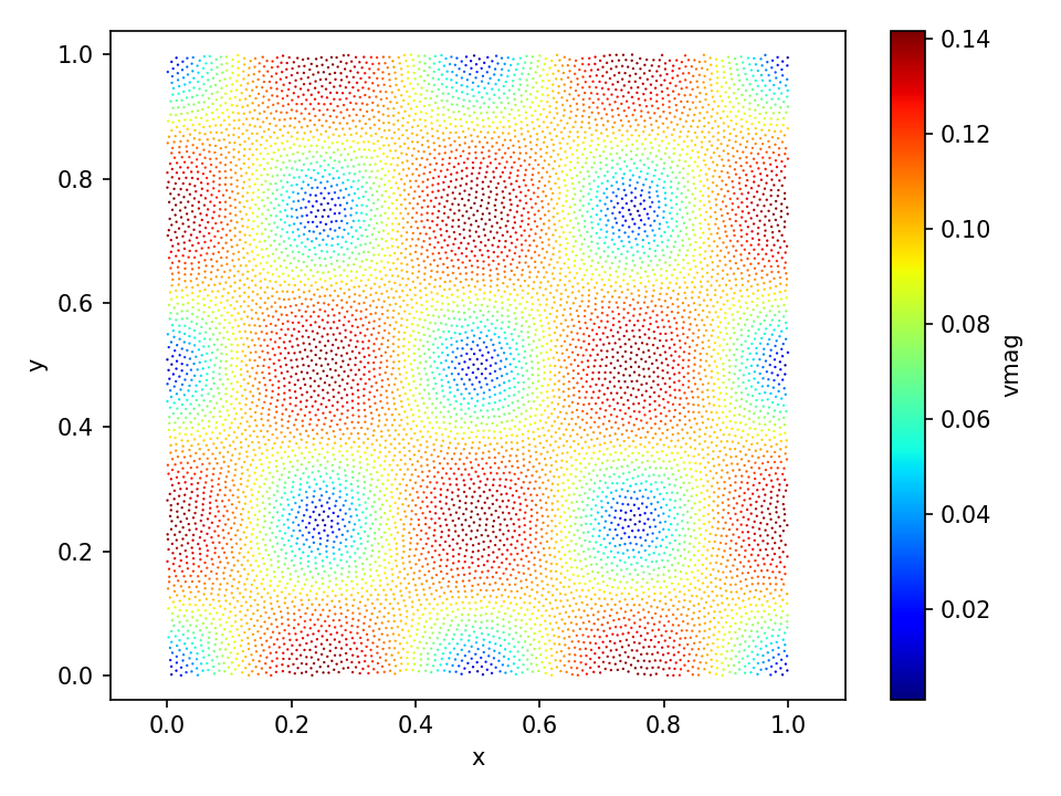
Figure 5: The distribution of particles at $t=2.5$ for the simulation using the EDAC scheme with $n_{x}=100$. The colors indicate the velocity magnitude.

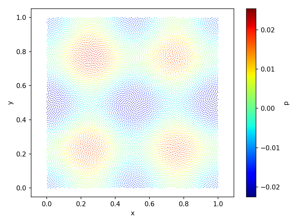
(a) EDAC scheme.

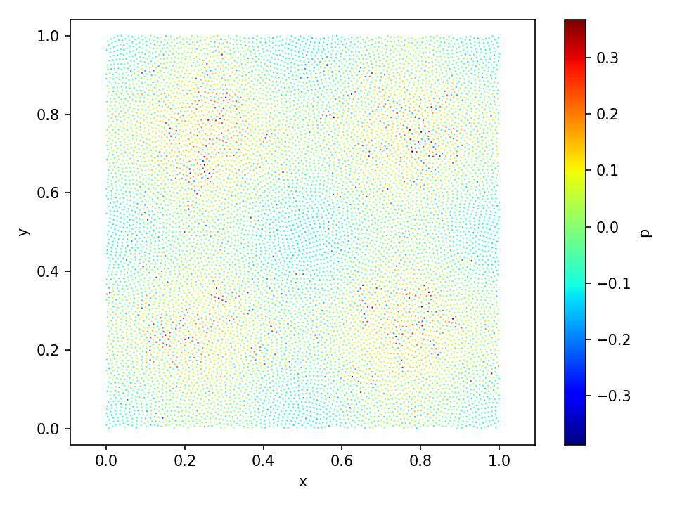
(b) TVF scheme.

Figure 6: The distribution of particles showing the pressure at $t=2.5$ with $n_{x}=100$. The left column shows the results using the EDAC and the right show the results with the TVF scheme.

In Fig. 7, the variation in density computed using the summation density is plotted versus time. The Reynolds number is chosen as 100 and $n_{x}=50$ for all schemes. The variation is computed as the difference between the maximum and minimum density at that time. The density is computed using the summation density for all the schemes. The WCSPH scheme uses a continuity equation to evolve the density. The EDAC scheme only evolves the pressure. The plot serves as a test of how well the volume is preserved by the schemes. The EDAC scheme is far superior to the WCSPH scheme. The TVF scheme uses the summation density to compute the density and displays the smallest density variations.

Figure 7: The variation in the density computed using the summation density versus time for the WCSPH scheme, the EDAC scheme, and the TVF. The number of particles are $n_{x}=50$ and $Re=100$.

In Fig. 8, the $L_{1}$ error for the velocity magnitude is plotted but for different values of the initial particle spacing $n_{x}$. We note that $n_{x}=25$ corresponds to a $\Delta x=0.04$. As can be seen, the EDAC scheme (Section 3.2) consistently produces less error than the TVF scheme at even such low resolutions.

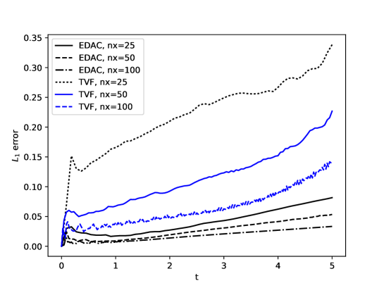
Figure 8: The $L_{1}$ error of the velocity magnitude versus $t$ for different resolutions.

From Fig. 8 it can be seen that with just $25\times 25$ particles, the EDAC produces about 3 times less error than the TVF. It is to be noted that for this low resolution, the random initial perturbation of the particles is limited to a maximum of $\Delta x/10$ instead of the $\Delta x/5$ for the other cases.

In order to study the sensitivity of the simulations to variations in the parameter $\alpha$ (equation 18) used for the diffusion of the pressure in the EDAC scheme, a few simulations with $n_{x}=25,Re=100$ for different values of $\alpha$ are performed. The results are shown in Fig. 9. For the variation of alpha by two orders of magnitude, the variation in the $L_{1}$ error is of the order of 0.04 which is less than the order of the error produced by the TVF scheme with 16 times as many particles. We perform a similar study with $Re=10000$ with a higher particle resolution and present the results in Fig. 15. From both these cases we are able to say that using an $\alpha$ of either 0.5 or 1.0 is reasonable.

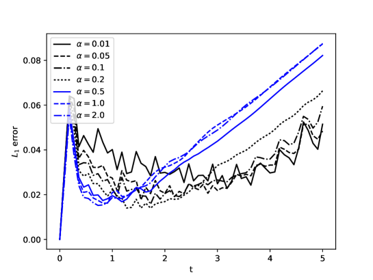
Figure 9: The $L_{1}$ error of the velocity magnitude versus $t$ for different choices of $\alpha$ with $Re=100,n_{x}=25$ while using the EDAC scheme.

Fig. 10 shows a convergence study for this problem with $Re=1000$ and $\alpha=1.0$. The particle spacing is increased from $n_{x}=25$ to $n_{x}=301$. Convergence in the $L_{1}$ norm for the velocity magnitude is seen in Fig. 11. The scheme appears to demonstrate first order convergence. However, it can be seen that when the $n_{x}$ is more than 200 the convergence rate drops. When a standard WCSPH scheme is used with a continuity equation the behavior is similar in that the convergence rate drops as the number of particles is increased. It is known [31, 32] that as the number of particles increase one must also increase the parameter $h$ such that the number of neighbors increase in order to have convergence. The results suggest that the new scheme is accurate, albeit suffering from the typical convergence related issues with traditional SPH schemes.

Figure 10: The $L_{1}$ error of the velocity magnitude versus $t$ for different choices of $n_{x}$ at $Re=1000$ while using the EDAC scheme.

In order to study the error variation as the parameter $h/\Delta x$ is changed, simulations are made at a $Re=1000$ with varying $n_{x}$ values. For this case, the Wendland Quintic (C2) kernel is used as it is best suited when increasing $h/\Delta x$ (see [33]). Fig. 12 plots the results obtained. The result clearly shows that as $h/\Delta x$ is increased, the accuracy increases and the convergence rate can be maintained.

Figure 11: The $L_{1}$ error of the velocity magnitude at $t=5$ versus $h$ at $Re=1000$ for the EDAC scheme. The dashed line shows the convergence of an ideal scheme with first order convergence.

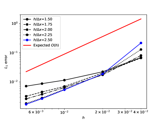
Figure 12: The $L_{1}$ error of the velocity magnitude versus $h$ at $t=2.5$ for different choices of $h/\Delta x$ at $Re=1000$ while using the EDAC scheme.

Figure 13: The distribution of particles at $t=5$ for the simulation using the EDAC scheme with $n_{x}=201$ at $Re=1000$. The colors indicate the velocity magnitude.

In Fig. 13 we plot the distribution of particles at the end of 5 seconds for the simulation at $Re=1000$ with $n_{x}=201$. This shows that the distribution of particles even at a very high resolution does not have any visible particle clustering.

It is useful to compare the performance of the proposed scheme at high Reynolds numbers. To this end, simulations are performed at $Re=10000$. A 100x100 grid of particles is used and with a small random initial perturbation to the particles (the maximum perturbation of $\Delta x/5$ is chosen). The TVF, EDAC external and EDAC TVF schemes are compared. As can be seen in Fig. 14, the new EDAC schemes perform very well. The EDAC TVF scheme (labeled as EDAC) significantly outperforms the TVF scheme. The standard EDAC scheme (Section 3.1) performs slightly better than the TVF.

Figure 14: The $L_{1}$ error of the velocity magnitude versus $t$ at $Re=10000$ for the different schemes, TVF, EDAC, and EDAC external.

In Fig. 15 the Reynolds number is set to 10000 with $n_{x}=101$ and $\alpha$ is varied. When $\alpha=0$, the physical viscosity is used. Clearly, much better results are produced when the suggested numerical viscosity value is used instead of the physical viscosity. When the suggested value is used the results are not too sensitive to changes in $\alpha$ around the value of $1$.

Figure 15: The $L_{1}$ error of the velocity magnitude versus $t$ for different choices of $\alpha$ at $Re=10000$ while using the EDAC scheme. When $\alpha=0$ is used the $\nu_{edac}$ is set to the fluid viscosity $\nu$.

The results show that the new scheme works well and outperforms the TVF. They justify the use of the numerical viscosity, equation (18), instead of the physical viscosity while diffusing the pressure. It is also important to note that unlike the TVF, the EDAC scheme works just as well when no initial random perturbation is given to the particles.

To provide some idea of the time taken for the simulation with different schemes we consider the case where $n_{x}=50$, and $Re=100$. Running the simulation up to $t=5s$ with the WCSPH took around 129 seconds, the TVF took 137 seconds, the standard EDAC took 151 seconds, and EDAC TVF formulation took 169 seconds. These simulations were made on a quad-core Intel i7-4770 CPU running at 3.4 GHz. The new scheme is about 25% slower than the standard WCSPH scheme which is reasonable considering the significant improvement in the results. However, the new scheme has not been optimized for performance and the above times are to illustrate the general performance.

4.2 Lid-Driven-Cavity

The next test problem considered is the classical Lid-Driven-Cavity (LDC) problem, which can be a fairly challenging problem to simulate with SPH. The setup is simple, a unit square box with no-slip walls on the bottom, left and right boundaries. The top wall is assumed to be moving with a uniform velocity, $V_{\text{lid}}$, which sets the Reynolds number for the problem ($Re=\frac{V_{\text{lid}}}{\nu}$). The present scheme is studied for two Reynold’s numbers $Re=100$, and $Re=1000$ and the results are compared to those of Ghia et al. [34].

The quintic spline kernel is used with $h=\Delta x$. The PEC type predictor-corrector integrator is used with a fixed time-step, chosen according to equation (26). In addition, $\alpha=0.5$ for all the SPH simulations. Since this problem does not involve free-surfaces, the TVF-EDAC scheme can be used (Section 3.2).

The discretization in terms of the number of particles is dependent on the Reynold’s number. A uniform distribution of particles ($\Delta x=\Delta y$) is used, with the maximum resolution of $50\times 50$, and $100\times 100$ for the $Re=100$, and $Re=1000$ cases respectively. The timesteps are chosen according to equation (26) as before. For each case, the code is run for a sufficiently long time to reach a steady state. This was found by looking at the kinetic energy of the entire fluid and checking if it is essentially constant. The velocity plots are made by averaging over the last $10$ saved time-step results. The data is saved every $500$ time-steps.

Fig. 16 shows the results for two different resolutions at $Re=100$ and Fig. 17 shows those for $Re=1000$. The results are in good agreement with those of Ghia et al. [34].

Figure 16: The velocity profiles $u$ vs. $y$ and $v$ vs. $x$ for the lid-driven-cavity problem at $Re=100$. The results are compared with those of Ghia et al. [34].

Figure 17: The velocity profiles $u$ vs. $y$ and $v$ vs. $x$ for the lid-driven-cavity problem at $Re=1000$. The results are compared with those of Ghia et al. [34].

4.3 Periodic lattice of cylinders

The next problem considered is a benchmark problem in a periodic square domain with a cylinder. The periodicity implies that the fluid effectively sees a periodic lattice of cylinders. This test was used to evaluate the TVF scheme in [11] and identical parameters are used for the numerical set-up. The length of the square domain is $L=0.1m$ and the Reynold’s number is set to one. A body force, $g_{x}=1.5\times 10^{-7}m/s^{2}$ drives the flow along the $x$ direction. The cylinder is placed in the center of the domain with a radius $R=0.02m$. The domain is periodic along both the coordination directions. A uniform discretization is used with $100\times 100$ particles and a quintic spline kernel with $h=\Delta x$ is used. The PEC type predictor-corrector integrator is used with a fixed time-step chosen using equation (26).

Fig. 18 shows the axial velocity profile ($u$) along the lines $x=L/2$ and $x=L$, when using the TVF-EDAC scheme and compare the results with the TVF scheme. The axial velocity is obtained by performing a Shepard interpolation of the fluid particle properties on points along the axial line. It is found that the results of the new scheme are in good agreement with that of the TVF scheme. For this problem the TVF simulation took around 198 seconds and the EDAC simulation took around 259 seconds.

Figure 18: Axial velocity profile ($u$) along the transverse ($y$) direction at $x=L/2$ and $x=L$ for the periodic lattice of cylinders using the EDAC (red) and TVF (black) schemes.

4.4 Periodic array of cylinders

The next benchmark is similar to the periodic lattice of cylinders but with no-slip wall boundary conditions along the top and bottom walls. The domain is periodic in the $x$ direction, driven by a body force $g_{x}=2.5\times 10^{-4}m/s^{2}$. A rigid cylinder with radius $R=0.2m$ is placed in the center of the channel. The length of the channel is $L=0.12m$ and the height is $H=4R$. The numerical set-up is identical to that of Adami et al. [11] with $n_{x}=144$ but with $h=1.2\Delta x$ chosen for both schemes. Fig. 19 shows the drag coefficient on the cylinder generated by the TVF and the new scheme. Fig. 20 shows the distribution of the particles at the final time produced by the EDAC scheme. The particles are homogeneously distributed as would be expected. The particle distribution is very similar to that produced by Adami et al. [11].

Note that for this problem, when using $c=0.1\sqrt{g_{x}R}$, as recommended by Adami et al. [11], the particle positions diverge when using the TVF formulation. Instead, in order to reproduce the results of Adami et al. [11] the value is set to $c=0.02m/s$ as recommended by Ellero and Adams [35].

The present results suggest that the EDAC scheme performs well for all of the internal flow cases. A few standard free-surface problems are considered next.

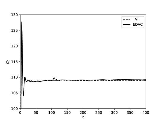
Figure 19: The drag variation $C_{D}$ versus time for a periodic array of cylinders in a channel. The results from the TVF (dash) are compared with those produced by the EDAC (solid) scheme.

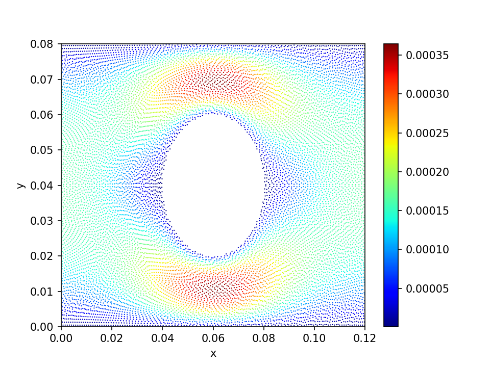
Figure 20: The distribution of particles at the final time produced by the EDAC scheme. The color indicates the velocity magnitude.

4.5 Elliptical drop

The elliptical drop problem is a classic problem that was first solved in the context of SPH by Monaghan [3]. The problem studies the evolution of a circular drop of inviscid fluid having unit radius in free space with the initial velocity field given by $-100x\hat{i}+100y\hat{j}$. No specific boundary conditions are applied on the outer surface of the elliptical drop as they are treated as a free surface. The incompressibility constraint on the fluid enables a derivation for evolution of the semi-major axis of the ellipse. The problem is simulated with the standard WCSPH scheme where an artificial viscosity with $\alpha=0.1$ is used. The particle spacing is chosen to be $\Delta x=0.025m$. A Gaussian kernel is used for the WCSPH with $h=1.3\Delta x$. The value of $\gamma=7$. The speed of sound is set to $1400m/s$ and $\rho=1.0kg/m^{3}$. For the EDAC case, a quintic spline kernel is used with $h=1.2\Delta x$. $\alpha=0.5$ for the calculation of $\nu_{edac}$. An Evaluate-Predict-Evaluate-Correct (EPEC) integration scheme is used for the WCSPH scheme whereas a Predict-Evaluate-Correct (PEC) integrator is used for the new scheme and the results are compared.

In Fig. 21, the semi-major axis of the ellipse is compared with the exact solution. The standard EDAC scheme (Section 3.1) is used to simulate the problem. No artificial viscosity is used for the EDAC scheme. Artificial viscosity is used for the WCSPH implementation with a value of $\alpha=0.1,\beta=0.0$. One EDAC simulation is performed using the XSPH correction [36] and one without it. Two additional cases of the EDAC along with the XSPH correction with a resolution of $\Delta x/2$ and $\Delta x/3$ are also performed. The absolute error in the size of the semi-major axis with time is used as a metric to compare the results. As can be seen, the EDAC scheme performs better than the standard SPH both with and without the XSPH correction.

Figure 21: The error in the computed size of the semi-major axis compared for the standard SPH, EDAC and the EDAC with the use of XSPH.

In Fig. 22, the kinetic energy of the fluid is computed and plotted versus time. It is to be noted that one may obtain the exact kinetic energy by integrating the initial velocity field. Given a unit density and an initial radius of unity, this amounts to approximately 7853.98 units. The kinetic energy of the standard SPH formulation reduces due to the artificial viscosity. The EDAC scheme on the other hand does not display any significant loss of kinetic energy and the value is close to the exact value.

Fig. 23(a) plots the particle distribution as obtained by the WCSPH simulation. The colors show the pressure distribution. The solid line is the exact solution. Fig. 23(b) shows the same obtained with the EDAC without the XSPH correction and Fig. 23(c) shows the particles and the pressure distribution using the EDAC scheme along with the XSPH correction. The XSPH correction seems to reduce the noise in the particle distribution. It is clear that the EDAC scheme has much lower pressure oscillations than the WCSPH scheme even though no artificial viscosity is used.

Figure 22: The kinetic energy of the elliptical drop computed by different schemes.

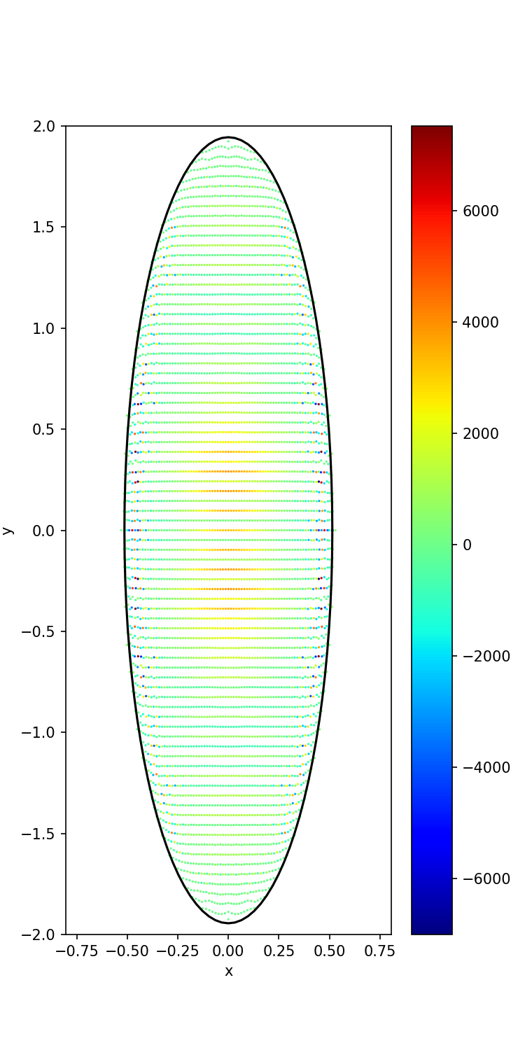
(a) WCSPH.

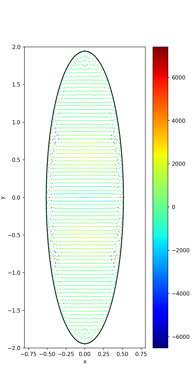
(b) EDAC no XSPH.

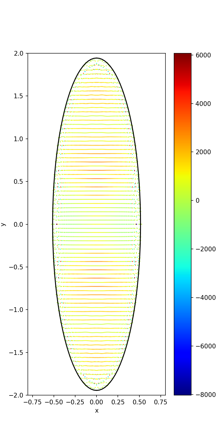
(c) EDAC with XSPH.

Figure 23: The distribution of particles for the elliptical drop problem at $t=0.0076$ seconds. The plot (a) is with the standard WCSPH scheme with the use of artificial viscosity. Plot (b) is with the EDAC without XSPH and (c) is EDAC with XSPH. The solid line is the exact solution and the colors indicated the pressure.

As can be seen, the new scheme outperforms the standard SPH scheme in general, conserves kinetic energy, has lower pressure oscillations, and is quite robust as there is no need for an artificial viscosity to keep the scheme stable.

4.6 Hydrostatic tank

The next example is a simple benchmark to ensure that the pressure is evolved correctly. This benchmark consists of a tank of water held at rest with the top of the vessel kept open as simulated by Adami et al. [26]. The fluid is initialized with a zero pressure with the particles at rest. The acceleration due to gravity is set to -1$m/s^{2}$, the height of the water is $0.9m$ and the density of the fluid is set to $1000kg/m^{3}$. The maximum speed of the fluid is taken to be $\sqrt{gH}$ and the speed of sound is set to ten times this value. The timestep is calculated as before using these values. The acceleration due to gravity is damped as discussed in [26]. In order to reproduce the results, the same artificial viscosity factor $\alpha=0.24$ is used. No physical viscosity is used. The parameter $\alpha$ for the EDAC equation is set to $0.5$. The problem is simulated with the TVF scheme (using no background pressure) as well as the EDAC scheme. No specific boundary condition is explicitly applied on the free surface. The walls of the tank are essentially slip-walls as the physical viscosity is zero. To compare the results, the pressure is evaluated along a line at the center of the tank.

In Fig. 24 the pressure at the bottom of the tank is plotted versus time for both the TVF scheme and the EDAC scheme. The EDAC scheme seems to produce a bit more oscillation in the pressure but the overall agreement is good.

Figure 24: Plot of the pressure at the bottom of the tank versus time for different schemes.

In Fig. 25, the pressure variation with height for a line of points at the center of the tank is plotted for different schemes at the times $t=0.5$ and $t=2$. The agreement is very good. This shows that the EDAC scheme produces accurate pressure distributions. In terms of execution time, the TVF simulation takes about 24 seconds and the EDAC simulation takes about 33 seconds.

Figure 25: Pressure variation with height for the different schemes at $t=0.5$ and $t=2.0$.

4.7 Water impact in two-dimensions

The case of two rectangular blocks of water impacting is considered next. A detailed study of this problem has been performed by Marrone et al. [37] in which they use a fully compressible, Riemann-Solver type SPH formulation and compare the results with a level-set finite volume method. The problem involves two blocks of water, each with side $H$ and height $L$, that are stacked vertically at $t=0$, with the interface at $y=0$. The top block moves down with the $y$-component of velocity $v=-U$ and the bottom moves up with velocity $v=U$. There is no acceleration due to gravity and the fluid is treated as inviscid and incompressible. Surface tension is not modeled. The surface of the blocks is treated as a free-surface. The problem is simulated using the standard EDAC scheme and also the WCSPH scheme. In the present case $L=1m$, $H=2m$, $U=1m/s$ and $\rho=1.0kg/m^{3}$. The Mach number is chosen to be $0.01$. For the WCSPH scheme, $\gamma=1$. A quintic spline kernel is used for both schemes with $h=\Delta x$ and $L/\Delta x=100$. As considered in [37], the normalized pressure distribution ($p/\rho c_{s}U$) is shown at $t^{*}=Ut/L=0.007$ and at $t^{*}=Ut/L=0.167$. When this case is run without any artificial viscosity, the traditional WCSPH scheme does not run successfully until the desired time. There are large pressure oscillations. Fig. 26 shows the particle distribution and pressure for the non-dimensionalized times of $t^{*}=0.007$ (left) and $t^{*}=0.1$ (right). In contrast, the EDAC case runs fairly well and the results are shown in Fig. 27. Initially, the pressure is comparable to the results in [37], however, the lack of any artificial viscosity results in small pressure oscillations at the final time and some cavitation. In Fig. 28 the same case is simulated with an artificial viscosity with $\alpha=0.1$. This produces fairly good results. It is easy to see that in all cases, the new scheme produces much less pressure oscillations. It is worth noting that while the WCSPH scheme requires the use of artificial viscosity for the simulation to complete, it displays high-frequency pressure oscillations as can be seen in Fig. 29, where the artificial viscosity parameter $\alpha=0.1$ was used for the WCSPH scheme. These results clearly show the superiority of the new scheme. In terms of performance, the WCSPH simulation takes about 211 seconds whereas the EDAC takes about 303 seconds. This is primarily because the EDAC implementation has not been fully optimized and due to the additional summation density computation that the EDAC requires.

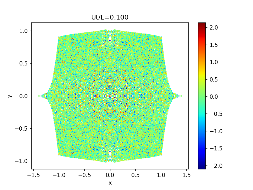
Figure 26: Particle distribution and pressure ($p/\rho c_{s}U$) at $Ut/L=0.007$ (left) and $Ut/L=0.1$ (right) for the water impact problem with the standard WCSPH scheme without any artificial viscosity.

Figure 27: Particle distribution and pressure ($p/\rho c_{s}U$) at $Ut/L=0.007$ (left) and $Ut/L=0.167$ (right) for simulation with the standard EDAC scheme without any artificial viscosity.

Figure 28: Particle distribution and pressure at $Ut/L=0.007$ (left) and $Ut/L=0.167$ (right) for simulation with the standard EDAC scheme with artificial viscosity coefficient $\alpha=0.1$.

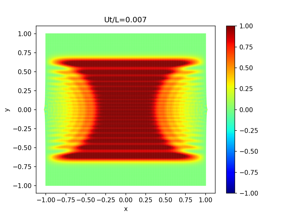
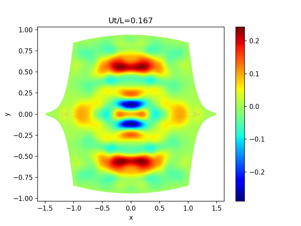
Figure 29: Particle distribution and pressure at $Ut/L=0.007$ (left) and $Ut/L=0.167$ (right) for simulation with the standard WCSPH scheme with artificial viscosity coefficient $\alpha=0.1$.

4.8 Dam-break in two-dimensions

The two-dimensional dam break over a dry bed is considered next. Results are instead compared with a standard SPH implementation. The suggested corrections of Hughes and Graham [38] and Marrone et al. [23] are also employed in the implementation of the standard SPH scheme as provided in PySPH. In the current work, only the corrections of Hughes and Graham [38] are used. The delta-SPH corrections of Marrone et al. [23] do not affect the present results.

The problem considered is as described in Gomez-Gesteria et al. [24] with a block of water $1m$ wide and $2m$ high, placed in a vessel of length $4m$. The block is released under the influence of gravity which is assumed to be $-9.81m/s^{2}$. The particles are arranged as per a staggered grid as is suggested for the standard SPH formulation by Gomez-Gesteria et al. [24] with $h=0.0156$. Artificial viscosity is used for the WCSPH implementation with a value of $\alpha=0.1,\beta=0.0$. The standard Wendland quintic kernel is used for WCSPH case with $h=1.3\Delta x$.

For the EDAC implementation, a uniform regular distribution of particles is used as done in [26]. No artificial viscosity or XSPH correction is employed. A quintic spline kernel is used with $h=\Delta x$. The value of $\alpha$ for the EDAC equation is set to $0.5$. The only change to the implementation is a clamping of the boundary pressure to non-negative values so as to prevent the fluid from sticking to the walls. At the highest resolution the EDAC simulation uses 8192 fluid particles whereas the WCSPH use 27889 particles due to the staggered grid arrangement.

To compare the results, the position of the toe of the dam versus time is plotted and compared with the results of the Moving Point Semi-implicit (MPS) scheme of [39]. The results are plotted in Fig. 30. As can be seen, the results of the new scheme compare well with the MPS results and the WCSPH formulation. The agreement is very good.

Figure 30: Position of the toe of the dam as a function of time compared with the MPS simulation of [39]. $Z$ is the distance of the toe of the dam from the left wall and $L$ is the initial width of the dam.

Fig. 31 shows the distribution of particles with the color indicating the pressure. The left panel shows the results obtained using the WCSPH scheme and the right shows that of the EDAC scheme. The top row is at 0.4 seconds and the bottom at 0.8 seconds. The fluid near the left wall is better behaved in the EDAC case and the surface is smooth. The EDAC scheme displays a larger amount of splashing due to the lack of any artificial viscosity in the momentum equation. Both schemes appear to show some noise near the left bottom wall at $t=0.4s$. The pressure magnitudes in the WCSPH case are much larger than those of the EDAC scheme.

Fig. 32 shows the velocity magnitude of the particles. The results are fairly similar. These results show that the new scheme works well for this problem. The EDAC scheme does not require the use of artificial viscosity in the momentum equation or the use of the XSPH correction.

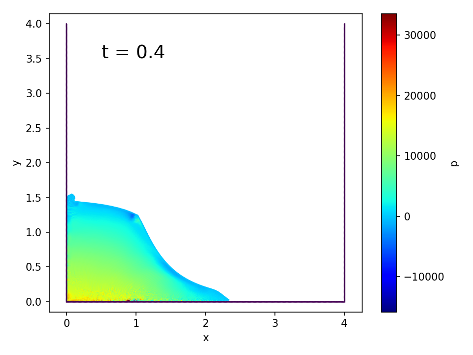
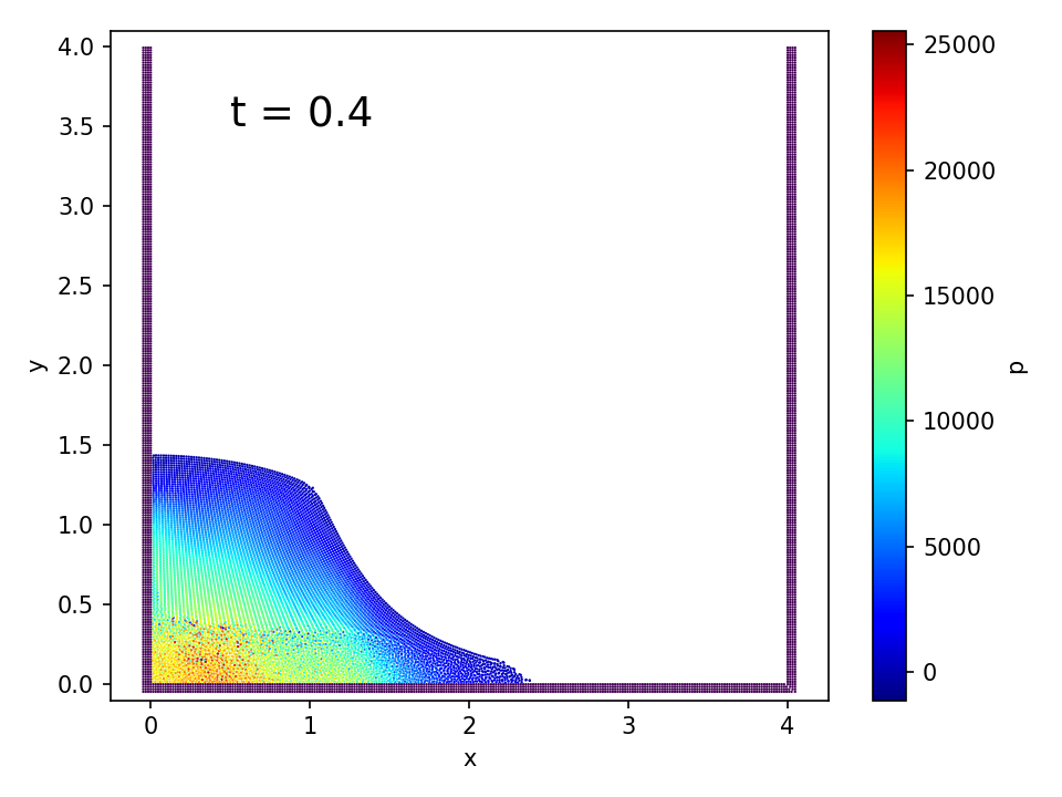
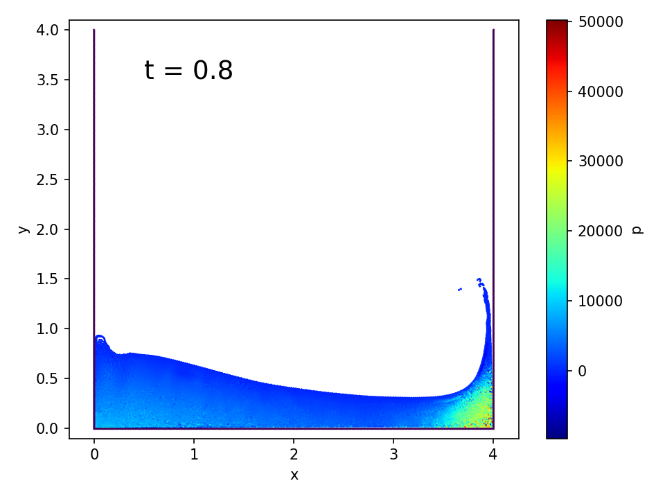
(a) WCSPH

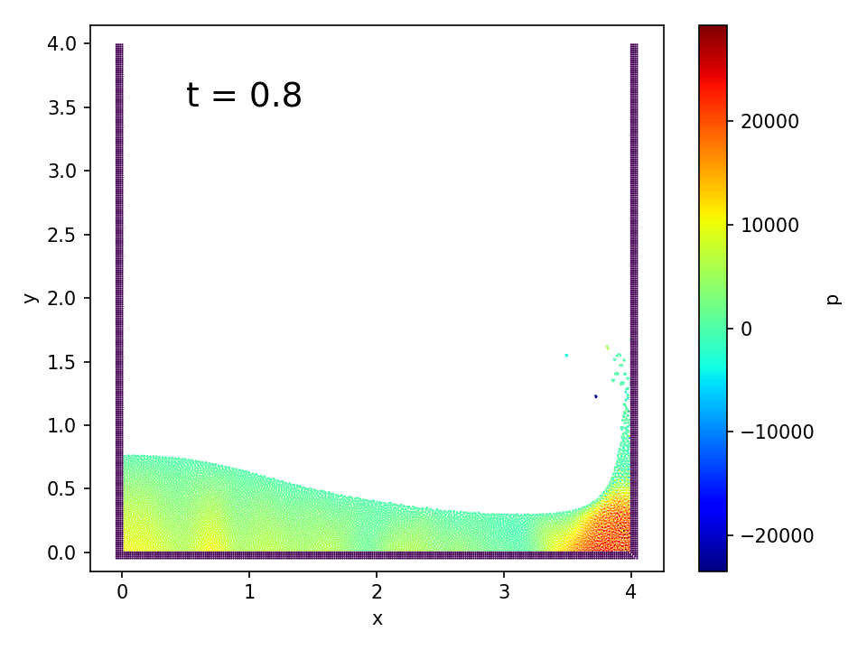
(b) EDAC

Figure 31: Particle distribution for the two-dimensional dam break problem, for the WCSPH and the EDAC cases. The WCSPH cases are on the left and the EDAC on the right. The color indicates the pressure. The top row is at a time of 0.4 seconds and the bottom at 0.8 seconds.

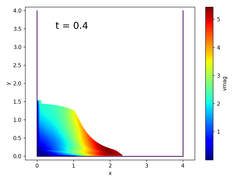
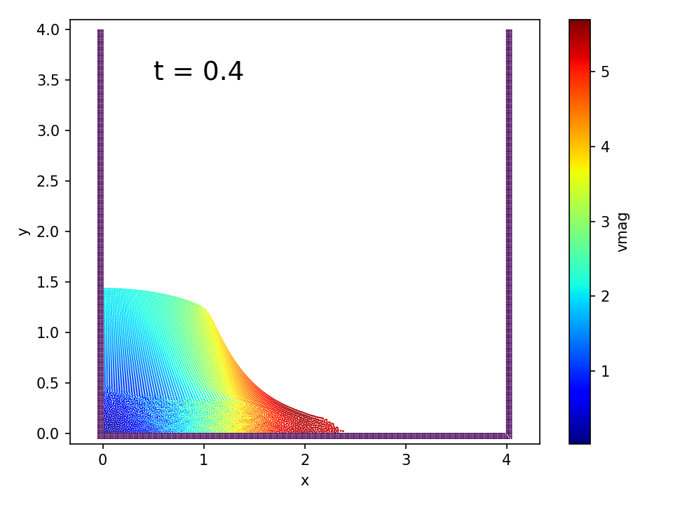
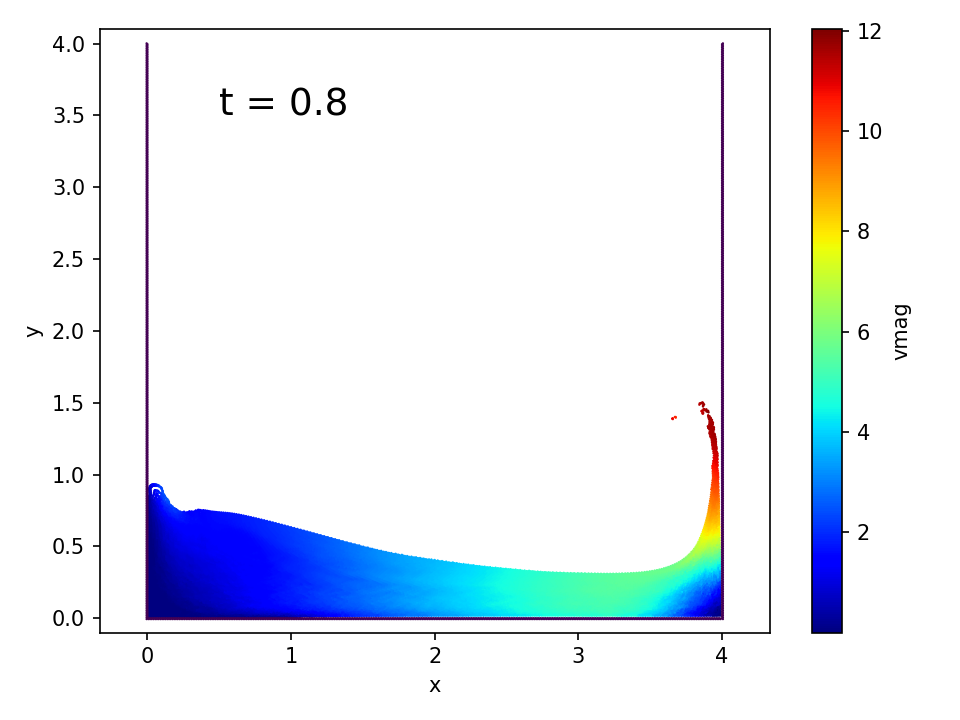
(a) WCSPH

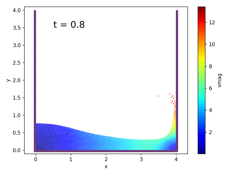
(b) EDAC

Figure 32: Particle distribution showing the velocity magnitude for the two-dimensional dam break problem, for the WCSPH and the EDAC cases. The WCSPH cases are on the left and the EDAC on the right. The top row is at a time of 0.4 seconds and the bottom at 0.8 seconds.

The benchmarks above show that the new scheme produces good results for internal and external flow problems.

5 Conclusions

In this work, the Entropically Damped Artificial Compressibility scheme of Clausen [13] is applied to SPH. Two flavors of the new scheme are developed, one called the EDAC TVF scheme which is suitable for internal flows, and the other called the standard EDAC scheme which is suitable for external flows. The key elements of the EDAC TVF scheme are the use of the EDAC equation to evolve the pressure, the use of the transport velocity formulation of Adami et al. [11], and, importantly, a pressure correction as suggested by Basa et al. [27]. This scheme outperforms the TVF scheme for the Taylor Green vortex problem at various Reynolds numbers. The scheme performs very well for a variety of other internal flow problems. The standard EDAC scheme is easy to apply to external flow problems and to free-surface flows. The method produces results that are better than the standard SPH. The pressure distribution is smoother and more accurate. It does not require the use of artificial viscosity and is relatively simple to implement. It is seen that a judicious choice of the viscosity for the pressure equation is important. A heuristic expression is suggested that appears to work well for all the simulated problems. While this viscosity introduces a new parameter, our computations suggest that this parameter does not need to be tuned for different problems and a value of 0.5 or 1.0 works well for a variety of Reynolds numbers and problems. A fully working implementation of the scheme and all the benchmarks in this paper are made freely available in order to encourage reproducible computational science.

References

References

- Lucy [1977] Lucy, L.B.. A numerical approach to testing the fission hypothesis. The Astronomical Journal 1977;82(12):1013–1024.
- Gingold and Monaghan [1977] Gingold, R.A., Monaghan, J.J.. Smoothed particle hydrodynamics: Theory and application to non-spherical stars. Monthly Notices of the Royal Astronomical Society 1977;181:375–389.
- Monaghan [1994] Monaghan, J.J.. Simulating free surface flows with SPH. Journal of Computational Physics 1994;110:399–406.
- Shadloo et al. [2016] Shadloo, M.S., Oger, G., Touze, D.L.. Smoothed particle hydrodynamics method for fluid flows, toward industrial applications: Motivations, current state, and challenges. Computers & Fluids 2016;136:11–34.
- Violeau and Rogers [2016] Violeau, D., Rogers, B.D.. Smoothed particle hydrodynamics (SPH) for free-surface flows: past, present and future. Journal of Hydraulic Research 2016;54:1–26.
- Cummins and Rudman [1999] Cummins, S.J., Rudman, M.. An SPH projection method. Journal of Computational Physics 1999;152:584–607.
- Shao and Lo [2003] Shao, S., Lo, E.Y.. Incompressible SPH method for simulating newtonian and non-newtonian flows with a free surface. Advances in Water Resources 2003;26(7):787 – 800. URL: http://www.sciencedirect.com/science/article/pii/S0309170803000307. doi:https://doi.org/10.1016/S0309-1708(03)00030-7.
- Hu and Adams [2007] Hu, X., Adams, N.. An incompressible multi-phase SPH method. Journal of Computational Physics 2007;227(1):264–278. URL: http://linkinghub.elsevier.com/retrieve/pii/S0021999107003300. doi:10.1016/j.jcp.2007.07.013.
- Ihmsen et al. [2014] Ihmsen, M., Cornelis, J., Solenthaler, B., Horvath, C., Teschner, M.. Implicit incompressible SPH. IEEE Trans Vis Comput Graph 2014;20(3):426–435. URL: https://doi.org/10.1109/TVCG.2013.105. doi:10.1109/TVCG.2013.105.
- Rouzbahani and Hejranfar [2017] Rouzbahani, F., Hejranfar, K.. A truly incompressible smoothed particle hydrodynamics based on artificial compressibility method. Computer Physics Communications 2017;210:10 – 28. URL: http://www.sciencedirect.com/science/article/pii/S001046551630279X. doi:https://doi.org/10.1016/j.cpc.2016.09.008.
- Adami et al. [2013] Adami, S., Hu, X., Adams, N.. A transport-velocity formulation for smoothed particle hydrodynamics. Journal of Computational Physics 2013;241:292–307. URL: http://linkinghub.elsevier.com/retrieve/pii/S002199911300096X. doi:10.1016/j.jcp.2013.01.043.
- Zhang et al. [2017] Zhang, C., Hu, X.Y.T., Adams, N.A.. A generalized transport-velocity formulation for smoothed particle hydrodynamics. Journal of Computational Physics 2017;337:216–232.
- Clausen [2013a] Clausen, J.R.. Entropically damped form of artificial compressibility for explicit simulation of incompressible flow. Physical Review E 2013a;87(1):013309–1–013309–12. URL: http://link.aps.org/doi/10.1103/PhysRevE.87.013309. doi:10.1103/PhysRevE.87.013309.
- Clausen [2013b] Clausen, J.R.. Developing Highly Scalable Fluid Solvers for Enabling Multiphysics Simulation. Tech. Rep. March; Sandia National Laborotories; 2013b. URL: http://prod.sandia.gov/techlib/access-control.cgi/2013/132608.pdf.
- Ansumali et al. [2005] Ansumali, S., Karlin, I.V., Öttinger, H.C.. Thermodynamic theory of incompressible hydrodynamics. Physical Review Letters 2005;94(8):1–4.
- Karlin et al. [2006] Karlin, I.V., Tomboulides, A.G., Frouzakis, C.E., Ansumali, S.. Kinetically reduced local Navier-Stokes equations: An alternative approach to hydrodynamics. Physical Review E 2006;74(3):6–9.
- Borok et al. [2007] Borok, S., Ansumali, S., Karlin, I.V.. Kinetically reduced local Navier-Stokes equations for simulation of incompressible viscous flows. Physical Review E 2007;76(6):1–9.
- Delorme et al. [2017] Delorme, Y.T., Puri, K., Nordström, J., Linders, V., Dong, S., Frankel, S.H.. A simple and efficient incompressible Navier-Stokes solver for unsteady and complex geometry flows on truncated domains. Computers & Fluids 2017;150:84–94.
- Ramachandran and Puri [2015] Ramachandran, P., Puri, K.. Entropically damped artificial compressibility for SPH. In: Liu, G.R., Das, R., eds. Proceedings of the 6th International Conference on Computational Methods 5 conference; vol. 2. Auckland, New Zealand; 2015:Paper ID 1210. URL: http://www.sci-en-tech.com/ICCM2015/PDFs/1210-3216-1-PB.pdf.
- Ramachandran and Puri [2013] Ramachandran, P., Puri, K.. PySPH: a framework for parallel particle simulations. In: Proceedings of the 3rd international conference on particle-based methods (Particles 2013). Stuttgart, Germany; 2013:.
- Ramachandran [2016] Ramachandran, P.. PySPH: a reproducible and high-performance framework for smoothed particle hydrodynamics. In: Benthall, S., Rostrup, S., eds. Proceedings of the 15th Python in Science Conference. 2016:127 – 135.
- Antuono et al. [2010] Antuono, M., Colagrossi, A., Marrone, S., Molteni, D.. Free-surface flows solved by means of SPH schemes with numerical diffusive terms. Computer Physics Communications 2010;181(3):532 – 549. doi:https://doi.org/10.1016/j.cpc.2009.11.002.
- Marrone et al. [2011] Marrone, S., Antuono, M., Colagrossi, A., Colicchio, G., Le Touzé, D., Graziani, G.. -SPH model for simulating violent impact flows. Computer Methods in Applied Mechanics and Engineering 2011;200:1526–1542. doi:10.1016/j.cma.2010.12.016.
- Gomez-Gesteria et al. [2010] Gomez-Gesteria, M., Rogers, B.D., Dalrymple, R.A., Crespo, A.J.. State-of-the-art classical SPH for free-surface flows. Journal of Hydraulic Research 2010;84:6–27.
- Morris et al. [1997] Morris, J.P., Fox, P.J., Zhu, Y.. Modeling low reynolds number incompressible flows using SPH. Journal of Computational Physics 1997;136(1):214–226. doi:http://dx.doi.org/10.1006/jcph.1997.5776.
- Adami et al. [2012] Adami, S., Hu, X., Adams, N.. A generalized wall boundary condition for smoothed particle hydrodynamics. Journal of Computational Physics 2012;231(21):7057–7075. URL: http://linkinghub.elsevier.com/retrieve/pii/S002199911200229X. doi:10.1016/j.jcp.2012.05.005.
- Basa et al. [2009] Basa, M., Quinlan, N.J., Lastiwka, M.. Robustness and accuracy of SPH formulations for viscous flow. International Journal for Numerical Methods in Fluids 2009;60:1127–1148.
- Ramachandran et al. [10 ] Ramachandran, P., Puri, K., et al. PySPH: a python-based SPH framework. 2010–. URL: http://pypi.python.org/pypi/PySPH/.
- Ramachandran [2018] Ramachandran, P.. automan: A python-based automation framework for numerical computing. Computing in Science & Engineering 2018;20(5):81–97. URL: doi.ieeecomputersociety.org/10.1109/MCSE.2018.05329818. doi:10.1109/MCSE.2018.05329818.
- Monaghan [2000] Monaghan, J.J.. SPH without a tensile instability. Journal of Computational Physics 2000;159:290–311.
- Robinson and Monaghan [2012] Robinson, M., Monaghan, J.J.. Direct numerical simulation of decaying two-dimensional turbulence in a no-slip square box using smoothed particle hydrodynamics. International Journal for Numerical Methods in Fluids 2012;70(1):37–55. URL: https://onlinelibrary.wiley.com/doi/abs/10.1002/fld.2677. doi:10.1002/fld.2677.
- Zhu et al. [2015] Zhu, Q., Hernquist, L., Li, Y.. Numerical convergence in smoothed particle hydrodynamics. The Astrophysical Journal 2015;800(1):6. URL: http://stacks.iop.org/0004-637X/800/i=1/a=6. doi:https://doi.org/10.1088/0004-637X/800/1/6.
- Dehnen and Aly [2012] Dehnen, W., Aly, H.. Improving convergence in smoothed particle hydrodynamics simulations without pairing instability. Monthly Notices of the Royal Astronomical Society 2012;425(2):1068–1082. URL: http://dx.doi.org/10.1111/j.1365-2966.2012.21439.x. doi:10.1111/j.1365-2966.2012.21439.x.
- Ghia et al. [1982] Ghia, U., Ghia, K.N., Shin, C.T.. High-Re solutions for incompressible flow using the Navier-Stokes equations and a multigrid method. Journal of Computational Physics 1982;48:387–411.
- Ellero and Adams [2011] Ellero, M., Adams, N.. SPH simulations of flow around a periodic array of cylinders confined in a channel. International Journal for Numerical Methods in Engineering 2011;86:1027–1040.
- Monaghan [1989] Monaghan, J.J.. On the problem of penetration in particle methods. Journal of Computational Physics 1989;82:1–15.
- Marrone et al. [2015] Marrone, S., Colagrossi, A., Di Mascio, A., Le Touzé, D.. Prediction of energy losses in water impacts using incompressible and weakly compressible models. Journal of Fluids and Structures 2015;54:802–822. doi:10.1016/j.jfluidstructs.2015.01.014.
- Hughes and Graham [2010] Hughes, J., Graham, D.. Comparison of incompressible and weakly-compressible SPH models for free-surface water flows. Journal of Hydraulic Research 2010;48:105–117.
- Koshizuka and Oka [1996] Koshizuka, S., Oka, Y.. Moving-particle semi-implicit method for fragmentation of incompressible fluid. Nuclear Science and Engineering 1996;123:421–434.