A Coordinate-Descent Framework to Design Low PSL/ISL Sequences

Abstract

This paper is focused on the design of phase sequences with good (aperiodic) autocorrelation properties in terms of Peak Sidelobe Level (PSL) and Integrated Sidelobe Level (ISL). The problem is formulated as a bi-objective Pareto optimization forcing either a continuous or a discrete phase constraint at the design stage. An iterative procedure based on the coordinate descent method is introduced to deal with the resulting optimization problems which are non-convex and NP-hard in general. Each iteration of the devised method requires the solution of a non-convex min-max problem. It is handled either through a novel bisection or an FFT-based method for the continuous and the discrete phase constraint, respectively. Additionally, a heuristic approach to initialize the procedures employing the $l_{p}$-norm minimization technique is proposed. Simulation results illustrate that the proposed methodologies can outperform some counterparts providing sequences with good autocorrelation features especially in the discrete phase/binary case.

I Introduction

Waveform design has received considerable attention during the last eight decades in many communication, active sensing, and electronic warfare systems [1]. In communication systems (e.g., code-division multiple access), low correlation sidelobes are desired for synchronization and reduction of multi-access interferences [2]. In radar range compression, low Peak Sidelobe Level (PSL) waveforms are employed to avoid masking of weak targets in the range sidelobes of a strong return [3, 4]. Besides, to mitigate the deleterious effects of distributed clutter returns close to the target of interest [5], signals with low Integrated Sidelobe Level (ISL) are exploited. Remarkably, coded waveforms and range compression grant enhanced electronic protection against barrage jamming as well as increased range resolution which is critical in electronic warfare, e.g., to prevent deceptive attacks based on range-gate pull-off [6]. Also, pulse to pulse changing the transmitted waveform totally counters range-gate pull-in attacks [6]. Generally speaking, according to the hardware technology involved in the waveform generation process, the signals employed in real systems can be classified in two types: analog and digital. The former class exploits analog circuits/devices and typical examples are the Linear Frequency Modulated (LFM) and the non-linear frequency modulated signals; the latter is based on arbitrary digital waveform generators and relevant instances are the phase coded waveforms involving Barker, Frank, and Golomb, sequences, just to list a few [7]. Both conventional phase coded and LFM waveforms are ubiquitous in practical systems mainly due to their easy generation as well as the possible tolerance to Doppler-shifts. Nevertheless, the static use of a fixed waveform could determine a scarce adaptivity to the operating environment as well as vulnerability to electronic attacks highlighting the need for multiple and diverse waveforms exhibiting specific features [8]. As a result, several researchers have proposed a variety of approaches based on sophisticated optimization methods to design advanced polyphase sequences [9, 10, 11, 12]. This paper is framed in the mentioned context with the goal of designing constant-modulus sequences whose autocorrelation sidelobes share a desirable behavior.

I-A Background and Previous Works

Binary phase coded waveforms are common in radar and communication systems being their implementation quite simple [13]. Important instances are the Barker codes which are unfortunately limited to length 13. $M$-sequences, well-known for their ideal periodic autocorrelation function, can be easily generated using linear feedback shift registers but have no constraints/guarantees on the sidelobes of their aperiodic autocorrelation function; hence, they are almost impractical in radar applications (similarly Gold codes and Kasami sequences). Unlike the case of periodic correlation, it is not possible to construct binary sequences with an exact impulsive aperiodic autocorrelation. Therefore, a brute-force approach to obtain good sequences is to perform an exhaustive search, viable especially when the alphabet size is small, i.e., binary case. Minimum Peak Sidelobe (MPS) sequences are the best binary codes in terms of PSL (known up to length 105) which are obtained via global search through some supercomputers; a summary of the best known binary sequences is presented in [14]. When the constellation size increases, it becomes difficult and difficult (almost impossible) to perform the exhaustive search. In these situations derivation of analytical methods to design optimal or nearly-optimal sequences are valuable. To this end, an Iterative Twisted appROXimation (ITROX) method is proposed in [15] to get discrete phase sub-optimal sequences with limited alphabet size. Heuristic techniques exploiting Simulated Annealing (SA), Threshold Accepting (TA), and Great Deluge Algorithm (GDA) have been developed to design generalized polyphase Barker sequences [16, 17, 18]. However, the maximum length of the obtained generalized Barker codes is limited to $77$ [19].
In [20] a computationally efficient cyclic optimization algorithm for the design of constant-modulus transmit signals with good auto- and cross-correlation features is developed with reference to Multi-Input-Multi-Output (MIMO) radars. Following a similar line of reasoning, in [21] and [9] cyclic algorithms for the minimization of ISL-related metrics in Single-Input-Single-Output (SISO) systems are introduced, i.e., Cyclic Algorithm Pruned (CAP), Cyclic Algorithm New (CAN), and Weighted CAN (WeCAN). The main merit of these procedures is the reduced computational complexity that leads to a quite short execution time. From a theoretical point of view, they are based on the solution of an optimization problem that is almost equivalent to the ISL minimization, being the objective function an approximation of the ISL. Recently, a new optimization algorithm which can directly minimize the ISL metric under a constant modulus constraint has been introduced in [12]. It relies on the Majorization-Minimization (MM) framework and generally converges to a locally optimum ISL value. Two different versions are proposed exploiting two distinct majorization functions (Majorization-minimization Weighted ISL (MWISL) and MWISL-Diag). Their performance in terms of achieved ISL values is similar to that of CAN algorithm. Meanwhile, adopting a suitable modification in both MWISL and MWISL-Diag (as specified in [12]), the aforementioned techniques can converge faster than CAN.
Most of the above literature is focused on ISL-oriented design problems mainly due to the technical difficulties arising when the non-differentiable and highly non-convex PSL metric is considered as figure of merit. A first attempt to fill this gap and systematically synthesize polyphase codes with low PSL values is pursued in [12]. Precisely, the authors provide an algorithm, based on MM paradigm, capable of minimizing the $l_{p}$-norm of the autocorrelation sidelobes. Hence, a heuristic method (called MM-PSL) exploiting the observation that the PSL coincides with the limit as $p$ goes to infinity of the mentioned $l_{p}$-norm is proposed to optimize the PSL.

I-B Contribution and Organization

In this paper, PSL and ISL, namely the two most important measures quantifying the quality of the autocorrelation function, are jointly considered to synthesize advanced constant modulus codes according to a Pareto optimization framework. Specifically, the problem is formulated as a bi-objective optimization where either a continuous or a discrete phase constraint is forced at the design stage. To tackle the resulting non-convex and, in general, NP-hard problems an iterative procedure based on the Coordinate Descent (CD) method is introduced. Each iteration of the developed procedure requires the solution of a non-convex min-max problem involving quartic functions. As to the continuous phase case, a novel polynomial-time bisection method aimed at solving globally the aforementioned problem is developed. The discrete phase design, encompassing the challenging binary synthesis, is handled via an FFT-based procedure. Besides, a heuristic approach to initialize the procedures exploiting an $l_{p}$-norm minimization criterion is introduced.

Summarizing, the contributions of this paper are:

• the development of an efficient CD method that optimizes an objective function given by a weighted sum of the ISL and PSL based metrics. The method decreases the value of the objective at each iteration and can ensure convergence to a stationary point provided that the Maximum Block Improvement (MBI) [24, 22] rule is adopted. Also, the complexity per iteration is polynomial. Remarkably, to the best of our knowledge, no mathematical algorithm with ensured convergence properties has been suggested in the literature for the exact PSL minimization.

• the design of sequences with discrete phase possessing low ISL and PSL. In this respect, it is worth observing that there exist algorithms in open literature for ISL minimization. Nevertheless, they usually do not perform well in the discrete phase case [20] and the proposed algorithm is able to outperform them. As to the PSL minimization, to the best of our knowledge, systematic approaches are not available in the open literature and our method fills this relevant gap.

• the specialization of the proposed design methodology to the context of binary sequences with good ISL and PSL. Precisely, at each iteration of the devised method a weighted sum of the ISL and the PSL based metrics of the starting binary code decreases until convergence.

The rest of this paper is organized as follows. Section II deals with problem formulation. In Section III, the CD-based solution method is introduced together with techniques aimed at solving the optimization problem involved in each iteration, for both the continuous and the discrete phase case. Besides, a heuristic method is discussed to initialize the new proposed algorithms. Numerical examples are provided in Section IV to illustrate the effectiveness of the approach. Finally, concluding remarks and possible future research tracks are given in Section V.

I-C Notation

We adopt the notation of using bold lowercase letters for vectors and bold uppercase letters for matrices. The transpose, the conjugate, and the conjugate transpose operators are denoted by the symbols ${(\cdot)^{T}}$, $(\cdot)^{*}$ and $(\cdot)^{H}$ respectively; The $l_{p}$-norm of a vector $x$ is denoted by $\|\mbox{\boldmath{$x$}}\|_{p}$. The letter $\jmath$ represents the imaginary unit (i.e., $\jmath=\sqrt{-1}$), while the letter $i$ often serves as index. For any complex number $x$, we use $\Re(x)$ and $\Im(x)$ to denote the real part and the imaginary part of $x$, respectively. For any $x\in\mathbb{R}$, $\lceil x\rceil$ denotes the lowest integer higher than or equal to $x$. Also, $|x|$ and $\arg(x)$ represent the modulus and the argument of $x$, respectively. The abbreviation “s.t.” stands for “subject to”.

II Problem Formulation

Let $\mbox{\boldmath{$x$}}=[x_{1},x_{2},\ldots,x_{N}]^{T}\in{\mathbb{C}}^{N}$ be the transmitted fast-time radar code vector with $N$ the number of coded sub-pulses (code length). The autocorrelation function associated with $x$ is defined as

$$r_{k}=\sum_{i=1}^{N-k}{x_{i}^{*}x_{i+k}},~{}~{}~{}~{}k=0,\ldots,N-1,$$ (1)

and represents the output of the matched filter to $x$ when $x$ is the input signal. The PSL and ISL metrics are commonly used to design waveforms with “good” autocorrelation properties [7] and are formally defined as

PSL $$= \max\{|r_{k}|\}_{k=1}^{k=N-1},$$ (2)

ISL $$= \sum_{k=1}^{N-1}|r_{k}|^{2},$$ (3)

respectively. This paper is focused on the design of unimodular sequences considering simultaneously the PSL and the ISL as performance indices. From an analytical point of view the problem can be formulated as the following constrained bi-objective optimizations,

$$P^{\infty}\begin{dcases}\min_{\mbox{\boldmath{$x$}}}&{f_{1}(\mbox{\boldmath{$x$}}),f_{2}(\mbox{\boldmath{$x$}})}\\ s.t.&\mbox{\boldmath{$x$}}\in\Omega_{\infty}\end{dcases} ,~{}~{}P^{M}\begin{dcases}\min_{\mbox{\boldmath{$x$}}}&{f_{1}(\mbox{\boldmath{$x$}}),f_{2}(\mbox{\boldmath{$x$}})}\\ s.t.&\mbox{\boldmath{$x$}}\in\Omega_{M}\end{dcases}$$ (4)

where

$$f_{1}{(\mbox{\boldmath{$x$}})}=\max\{|r_{k}|^{2}\}_{k=1}^{k=N-1}$$

and

$$f_{2}{(\mbox{\boldmath{$x$}})}=\sum_{k=1}^{k=N-1}\{|r_{k}|^{2}\}.$$

Herein, the constraints $\mbox{\boldmath{$x$}}\in\Omega_{\infty}$ and $\mbox{\boldmath{$x$}}\in\Omega_{M}$ denote continuous alphabet and finite alphabet codes, respectively. Precisely,

$$\Omega_{\infty}=\{\mbox{\boldmath{$x$}}\in{\mathbb{C}}^{N}|~{}|x_{i}|=1,i=1,\ldots,N\}$$ (5)

and

$$\Omega_{M}=\{\mbox{\boldmath{$x$}}|x_{i}\in\Psi_{M},i=1,\ldots,N\},$$ (6)

where $\Psi_{M}=\{1,\bar{\omega},\ldots,\bar{\omega}^{M-1}\}$, $\bar{\omega}=e^{\jmath\frac{2\pi}{M}}$ and $M$ is the size of discrete constellation alphabet.
In a multi-objective optimization framework, usually a feasible solution that minimizes all the objective functions simultaneously does not exist [25]. Accordingly, the goal is to find the Pareto-optimal solutions to (4) which is in general a formidable task. A viable means to obtain the above solutions is the scalarization technique which exploits as objective a specific weighted sum between $f_{1}{(\mbox{\boldmath{$x$}})}$ and $f_{2}{(\mbox{\boldmath{$x$}})}$. Specifically, defining the function $f_{\theta}(\mbox{\boldmath{$x$}})$, parameterized in the Pareto weight $\theta\in[0,1]$,

$$f_{\theta}(\mbox{\boldmath{$x$}})= ~{}{\theta f_{1}(\mbox{\boldmath{$x$}})+(1-\theta)f_{2}(\mbox{\boldmath{$x$}})}$$

$$= \displaystyle{\max_{k=1,\ldots,N-1}}\left[\theta{|r_{k}|^{2}}+(1-\theta)\sum_{l=1}^{N-1}{|r_{l}|^{2}}\right]$$ (7)

scalarization leads to the design problems

$$P^{\infty,\theta}\begin{dcases}\min_{\mbox{\boldmath{$x$}}}&f_{\theta}(\mbox{\boldmath{$x$}})\\ s.t.&\mbox{\boldmath{$x$}}\in\Omega_{\infty}\end{dcases} ,P^{M,\theta}\begin{dcases}\min_{\mbox{\boldmath{$x$}}}&f_{\theta}(\mbox{\boldmath{$x$}})\\ s.t.&\mbox{\boldmath{$x$}}\in\Omega_{M}\end{dcases}$$ (8)

They reduce to pure ISL (PSL) minimization setting $\theta=0$ ($\theta=1$). Moreover, for any $\theta$, an optimal solution to (8) is a Pareto-optimal point to Problem (4) (see [27, 28, 26] and references therein for details).

III CD Code Optimization

This section introduces an iterative algorithm based on the CD minimization procedure [29] (also known as alternate optimization [30]) to sequentially optimize our objective over one variable keeping fixed the others. Otherwise stated, according to the CD approach, the minimization of a multivariable function can be achieved minimizing it along one direction at a time, i.e., solving univariate optimization problems in a loop [29, 31]. With reference to (8), at each iteration a specific code entry is selected as variable to optimize leading to the following problems at step $n+1$

$$P^{\infty,\theta}_{d,\mbox{\boldmath{$x$}}^{(n)}}\begin{dcases}\min_{x_{d}}&f_{\theta}(x_{d};\mbox{\boldmath{$x$}}_{-d}^{(n)})\\ s.t.&|x_{d}|=1\end{dcases} ,P^{M,\theta}_{d,\mbox{\boldmath{$x$}}^{(n)}}\begin{dcases}\min_{x_{d}}&f_{\theta}(x_{d};\mbox{\boldmath{$x$}}_{-d}^{(n)})\\ s.t.&x_{d}\in\Omega_{M}\end{dcases}$$

where $x_{d}$ is the variable to optimize, ${\mbox{\boldmath{$x$}}_{-d}^{(n)}=[x_{1}^{(n)},\ldots,x_{d-1}^{(n)},x_{d+1}^{(n)},\ldots,x_{N}^{(n)}]^{T}\in{\mathbb{C}}^{N-1}}$ refers to the remaining code entries, and

$$f_{\theta}(x_{d};\mbox{\boldmath{$x$}}_{-d}^{(n)})=f_{\theta}(x_{1}^{(n)},\ldots,x_{d-1}^{(n)},x_{d},x_{d+1}^{(n)},\ldots,x_{N}^{(n)}).$$

Thus, denoting by $x_{d,n+1}^{\star}$ the optimal solution to either $P^{\infty,\theta}_{d,\mbox{\boldmath{$x$}}^{(n)}}$ or $P^{M,\theta}_{d,\mbox{\boldmath{$x$}}^{(n)}}$, the optimized radar code at step $n+1$ is $\mbox{\boldmath{$x$}}^{(n+1)}=[x_{1}^{(n)},\ldots,x_{d-1}^{(n)},x_{d,n+1}^{\star},x_{d+1}^{(n)},\ldots,x_{N}^{(n)}]^{T}$. As a result, starting from an initial code $\mbox{\boldmath{$x$}}^{(0)}$ a sequence $\mbox{\boldmath{$x$}}^{(1)},\mbox{\boldmath{$x$}}^{(2)},\mbox{\boldmath{$x$}}^{(3)},\ldots$ of radar codes are obtained iteratively. A summary of the proposed approach can be found in Algorithm 1.

Algorithm 1 Continuous (Discrete) Phase Code Design with Good Autocorrelation Features

Input: Initial code $\mbox{\boldmath{$x$}}_{0}\in\Omega_{\infty}$ ($\mbox{\boldmath{$x$}}_{0}\in\Omega_{M}$), $\theta\in[0,1]$, and minimum required improvement $\epsilon$;
Output: Optimal solution $\mbox{\boldmath{$x$}}^{\star}$;

1. Initialization.

   • Compute the initial objective value ${f_{\theta}(x^{(0)}_{1},x^{(0)}_{2},\ldots,x^{(0)}_{N})}$ using equation (II);

   • Set $d:=1$ and $n:=0$;

2. Improvement.

   • Solve $P^{\infty,\theta}_{d,\mbox{\boldmath{$x$}}^{(n)}}$ ($P^{M,\theta}_{d,\mbox{\boldmath{$x$}}^{(n)}}$) obtaining $x_{d}^{\star}$;

   • Set ${n:=n+1}$ and
     ${\mbox{\boldmath{$x$}}^{(n)}\!=\!\left[x_{1}^{(n-1)},\ldots,x_{d-1}^{(n-1)}\!,\!x_{d}^{\star},x_{d+1}^{(n-1)}\!,\ldots,x_{N}^{(n-1)}\!\right]^{T}}\!$;

3. Stopping Criterion.

   • If $|f_{\theta}(\mbox{\boldmath{$x$}}^{(n)})-f_{\theta}(\mbox{\boldmath{$x$}}^{(n-1)})|\ <\epsilon$, stop. Otherwise, update $d$, i.e., if $d<N$ $d=d+1$, otherwise $d=1$, and go to the step 2;

4. Output.

   • Set $\mbox{\boldmath{$x$}}^{\star}=\mbox{\boldmath{$x$}}^{(n)}$.

Notice that, the monotonic property of the CD technique along with the fact that the objective function is bounded (from below) are sufficient to prove the convergence of the sequence of objective values. It is also worth pointing out that the Maximum Block Improvement (MBI) updating rule [24] can be used in place of the cyclic one (actually involved in Algorithm 1) to ensure the convergence of the algorithm to a stationary point. In practice, a final optimized code can be obtained refining the solution provided Algorithm 1 through the MBI-modification.
To proceed further, let us make explicit the functional dependence of the objective function in $P^{\infty,\theta}_{d,\mbox{\boldmath{$x$}}^{(n)}}$ ($P^{M,\theta}_{d,\mbox{\boldmath{$x$}}^{(n)}}$), i. e., $f_{\theta}(x_{d};\mbox{\boldmath{$x$}}_{-d}^{(n)})$ over the optimization variable $x_{d}$, i.e.,

$$r_{k}(x_{d})= x_{d}x_{d+k}^{*}\mathbf{1}_{A}(d+k)+x_{d-k}x_{d}^{*}\mathbf{1}_{A}(d-k)$$ (9)

$$+\sum_{i=1,i\neq\{d,d-k\}}^{N-k}{x_{i}x_{i+k}^{*}},~{}k=1,\ldots,N-1,$$

where $\mathbf{1}_{A}(.)$ denotes the indicator function of the set $A=\{1,2,\ldots,N\}$, i.e., $\mathbf{1}_{A}(x)=1$ if $x\in A$, otherwise $\mathbf{1}_{A}(x)=0$. Defining, $a_{dk}\triangleq x_{d+k}^{*}\mathbf{1}_{A}(d+k)$, $b_{dk}\triangleq x_{d-k}\mathbf{1}_{A}(d-k)$ and $c_{dk}\triangleq\sum_{i=1,i\neq\{d,d-k\}}^{N-k}{x_{i}x_{i+k}^{*}}$, the autocorrelation function with the explicit $x_{d}$-dependence can be written as

$$r_{k}(x_{d})=a_{dk}x_{d}+b_{dk}x_{d}^{*}+c_{dk},~{}~{}~{}k=1,\ldots,N-1.$$ (10)

Thus, the optimization problems $P^{\infty,\theta}_{d,\mbox{\boldmath{$x$}}^{(n)}}$ and $P^{M,\theta}_{d,\mbox{\boldmath{$x$}}^{(n)}}$ can be recast as,

$$P^{\infty,\theta}_{d,\mbox{\boldmath{$x$}}^{(n)}}\begin{dcases}\min_{x_{d}}\displaystyle{\max_{k=1,\ldots,N-1}}&\!\!\!\!\left[\theta{\left|{r_{k}(x_{d})}\right|^{2}}+(1-\theta)\!\!\sum_{l=1}^{N-1}{\left|{r_{l}(x_{d})}\right|^{2}}\right]\\ s.t.&|x_{d}|=1\end{dcases}$$

$$P^{M,\theta}_{d,\mbox{\boldmath{$x$}}^{(n)}}\begin{dcases}\min_{x_{d}}\displaystyle{\max_{k=1,\ldots,N-1}}&\!\!\!\!\left[\theta{\left|{r_{k}(x_{d})}\right|^{2}}+(1-\theta)\!\!\sum_{l=1}^{N-1}{\left|{r_{l}(x_{d})}\right|^{2}}\right]\\ s.t.&x_{d}\in\left\{1,e^{\jmath\frac{2\pi}{M}},\ldots,e^{\jmath\frac{2\pi(M-1)}{M}}\right\}\end{dcases}$$

which are non-convex, constrained, min-max problems with non-homogeneous quadratic objectives of a complex variable. In the next subsections, efficient algorithms to tackle $P^{\infty,\theta}_{d,\mbox{\boldmath{$x$}}^{(n)}}$ and $P^{M,\theta}_{d,\mbox{\boldmath{$x$}}^{(n)}}$ are derived. This issue represents the main technical innovation of this paper from an optimization theory point of view.

III-A Continuous Phase Code Design

This subsection is focused on the solution of Problem $P^{\infty,\theta}_{d,\mbox{\boldmath{$x$}}^{(n)}}$. As first step toward this goal, it is shown that the square modulus of the autocorrelation function at each lag (as a function of $x_{d}=e^{\jmath\phi_{d}},\phi_{d}\in[0,2\pi]$) can be expressed as the the ratio of two quartic functions of a real variable. This result is given in terms of the following

Lemma III.1.

Performing the change of variable $\beta_{d}\triangleq\tan\left({\frac{\phi_{d}}{2}}\right)$,

$$|\widetilde{r}_{k}(\beta_{d})|^{2} =|r_{k}(e^{\jmath\phi_{d}})|^{2}$$ (11)

$$=\frac{\mu_{dk}\beta_{d}^{4}+\kappa_{dk}\beta_{d}^{3}+\xi_{dk}\beta_{d}^{2}+\eta_{dk}\beta_{d}+\rho_{dk}}{(1+\beta_{d}^{2})^{2}},$$

where $\mu_{dk},\kappa_{dk},\xi_{dk},\eta_{dk},\rho_{dk}$ are real-valued coefficients depending on $a_{dk}$, $b_{dk}$ and $c_{dk}$ as specified in Appendix A.

Proof.

see Appendix A. ∎

Based on Lemma III.1, Problem $P^{\infty,\theta}_{d,\mbox{\boldmath{$x$}}^{(n)}}$ is equivalent to the following optimization problem,

$$\bar{P}^{\infty,\theta}_{d,\beta_{d}}\begin{dcases}\min_{\beta_{d}\in{\cal{R}}}&\displaystyle{\max_{k=1,\ldots,N-1}}\frac{\widetilde{p}_{k}(\beta_{d})}{\widetilde{q}(\beta_{d})}\end{dcases}$$ (12)

where

$$\widetilde{p}_{k}(\beta_{d})={\theta{p}_{k}(\beta_{d})+(1-\theta)\sum_{l=1}^{N-1}{p}_{l}(\beta_{d})}$$ (13)

and

$$\widetilde{q}(\beta_{d})=(1+\beta_{d}^{2})^{2},$$ (14)

with

$${p}_{k}(\beta_{d})=\mu_{dk}\beta_{d}^{4}+\kappa_{dk}\beta_{d}^{3}+\xi_{dk}\beta_{d}^{2}+\eta_{dk}\beta_{d}+\rho_{dk}.$$ (15)

In particular, ${\widetilde{p}_{k}(\beta_{d})}$ and ${\widetilde{q}(\beta_{d})}$ are non-negative quartic polynomials. Now, let $\bar{\gamma}\in{\cal{R}}^{+}$ be an slack variable and $v^{\star}$ the optimal value of the min-max optimization Problem $\bar{P}^{\infty,\theta}_{d,\beta_{d}}$ whose existence is ensured by Weierstrass theorem applied to $P^{\infty,\theta}_{d,\mbox{\boldmath{$x$}}^{(n)}}$. It can be checked whether the optimal value $v^{\star}$ is lower than or equal to a given value $\bar{\gamma}$ solving the feasibility problem

$$\widetilde{P}^{\infty,\theta}_{\beta_{d},\bar{\gamma}}\begin{dcases}\text{find}&\beta_{d}\\ s.t.&\frac{\widetilde{p}_{k}(\beta_{d})}{\widetilde{q}(\beta_{d})}\leq{\bar{\gamma}},~{}~{}k=1,\ldots,N-1\end{dcases}$$ (16)

If $\widetilde{P}^{\infty,\theta}_{\beta_{d},\bar{\gamma}}$ is feasible, then $v^{\star}\leq\bar{\gamma}$ and there exists a point in the feasible set achieving an objective value better than or equal to $\bar{\gamma}$. Conversely, if Problem $\widetilde{P}^{\infty,\theta}_{\beta_{d},\bar{\gamma}}$ is infeasible $v^{\star}\geq\bar{\gamma}$. The above observation paves the way to the development of an efficient iterative algorithm to solve $\bar{P}^{\infty,\theta}_{d,\beta_{d}}$ according to the bisection approach [26]. Precisely, at step $i$ the feasibility Problem (16) is solved with $\bar{\gamma}=\frac{u_{(i)}+w_{(i)}}{2}$ where $[w_{(i)},u_{(i)}]$ is the current interval containing the optimal value $v^{\star}$. Based on the feasibility check, it is possible to determine whether the optimal value is in the lower or in the upper half of the current interval and update the search accordingly with a consequent uncertainty halving. The procedure is repeated until the width of the interval is lower than or equal to a prescribed accuracy.
To study the feasibility of $\widetilde{P}^{\infty,\theta}_{d,\beta_{d}}$ for a given $\bar{\gamma}$, let us define the feasible set ${\cal{A}}_{k}^{\bar{\gamma}}$ as,

$${\cal{A}}_{k}^{\bar{\gamma}}=\left\{\beta_{d}|\left[\widetilde{p}_{k}(\beta_{d})-\bar{\gamma}\widetilde{q}(\beta_{d})\right]\leq 0\right\},k=1,\ldots,N-1,$$ (17)

and the complement set $\overline{\cal{A}}_{k}^{\bar{\gamma}}$ as,

$$\overline{\cal{A}}_{k}^{\bar{\gamma}}=\left\{\beta_{d}|\left[\widetilde{p}_{k}(\beta_{d})-\bar{\gamma}\widetilde{q}(\beta_{d})\right]>0\right\},k=1,\ldots,N-1.$$ (18)

Therefore $\widetilde{P}^{\infty,\theta}_{d,\beta_{d}}$ is feasible if and only if,

$$\bigcap_{k=1}^{N-1}{\cal{A}}_{k}^{\bar{\gamma}}\neq\varnothing\Leftrightarrow\overline{\bigcup_{k=1}^{N-1}\overline{\cal{A}}_{k}^{\bar{\gamma}}}\neq\varnothing\Leftrightarrow{\bigcup_{k=1}^{N-1}\overline{\cal{A}}_{k}^{\bar{\gamma}}}\neq{\cal{R}}.$$ (19)

Conversely, if ${\cup_{k=1}^{N-1}\overline{\cal{A}}_{k}^{\bar{\gamma}}}={\cal{R}}$ Problem $\widetilde{P}^{\infty,\theta}_{d,\beta_{d}}$ is infeasible. In a nutshell, to perform the feasibility check it is enough to compute the union of the intervals $\overline{{\cal{A}}}_{k}^{\bar{\gamma}}$ defined in (18) and to check for the possible gaps. In this respect, an efficient technique to establish the presence of gaps can be developed just finding the roots of $\widetilde{p}_{k}(\beta_{d})-\bar{\gamma}\widetilde{q}{(\beta_{d})},$ $k=1,\ldots,N$ (see Appendix B for details). A summary of the complete procedure to optimize an arbitrary entry of the phase code is provided in Algorithm 2.

Algorithm 2 Continuous Phase Code Entry Optimization

Input: Initial code vector $\mbox{\boldmath{$x$}}^{(n)}$, code entry $d$, $\theta$, and accuracy $\epsilon_{1}$;
Output: Optimal solution $x_{d}^{\star}$;

1. Compute $u=f_{\theta}\left(\mbox{\boldmath{$x$}}^{(n)}\right)$ as well as $\beta_{d}=\tan\left(\frac{\arg(x_{d}^{(n)})}{2}\right)$, and set $w=0$;

2. do

   1. $\bar{\gamma}=\frac{u+w}{2}$;

   2. $\overline{\cal{A}}_{k}^{\bar{\gamma}}=\left\{\beta_{d}:\left[\widetilde{p}_{k}(\beta_{d})-\bar{\gamma}\widetilde{q}(\beta_{d})\right]>0\right\}$;

   3. if ${\bigcup_{k=1}^{N-1}\overline{\cal{A}}_{k}^{\bar{\gamma}}}\neq{\cal{R}}$, $u=\bar{\gamma}$ and pick up a feasible solution $\beta_{d}$; else $w=\bar{\gamma}$;

3. until $u-w\leq\epsilon_{1}$;

4. Set $\phi^{\star}_{d}=2\mbox{atan}\left(\beta_{d}^{\star}\right)$, with $\beta_{d}^{\star}$ the obtained $\epsilon_{1}$-optimal solution;

5. Set $x_{d}^{\star}=e^{\jmath\phi^{\star}_{d}}$.

Remark 1. To establish the computational complexity of Algorithm 2 it is necessary to observe that the main actions in its implementation are:

1. calculation of ${\cup_{k=1}^{N-1}\overline{\cal{A}}_{k}^{\bar{\gamma}}}$;

2. bisection iterations;

3. evaluation of the optimal phase.

Calculation of $\overline{\cal{A}}_{k}^{\bar{\gamma}}$, $k=1,\ldots,N-1$, involves the evaluation of the roots of the fourth order polynomial $\widetilde{p}_{k}(\beta_{d})-\bar{\gamma}\widetilde{q}(\beta_{d})$ which can be done in closed form via Cardano’s procedure [32]. Hence, ${\cup_{k=1}^{N-1}\overline{\cal{A}}_{k}^{\bar{\gamma}}}$ can be obtained ordering the resulting real roots (possibly merging some overlapping intervals) with an overall computational complexity ${\cal{O}}(N\log_{2}(N))$ in the worst case [33]. As to the bisection method, in each iteration the search interval is divided in two parts. As a consequence, the interval size after $\bar{n}$ iterations is $2^{-\bar{n}}(u_{(0)}-w_{(0)})$. It follows that ${\cal{K}}=\lceil\log_{2}{(\frac{u_{(0)}-w_{(0)}}{\epsilon_{1}})}\rceil$ iterations are required before the algorithm terminates. Finally, since each step involves the solution of $\widetilde{P}_{d,\beta_{d}}^{\infty,\theta}$, the overall complexity is ${\cal{O}}({\cal{K}}N\log_{2}(N))$.

III-B Discrete Phase Code Design

Let us now consider Problem $P^{M,\theta}_{d,\mbox{\boldmath{$x$}}^{(n)}}$ and develop an efficient procedure to find its optimal solution exploiting Discrete Fourier Transform (DFT). In terms of $\phi_{d}=\arg(x_{d})$, $P^{M,\theta}_{d,\mbox{\boldmath{$x$}}^{(n)}}$ can be recast as,

$$\widetilde{P}^{M,\theta}_{d,\phi_{d}}\begin{dcases}\min_{\phi_{d}}&g_{\theta}(\phi_{d})\\ s.t.&\phi_{d}\in\mbox{\boldmath{$\phi$}}_{M}\end{dcases}$$ (20)

where $\mbox{\boldmath{$\phi$}}_{M}\triangleq\bigg{\{}0,\frac{2\pi}{M},\frac{4\pi}{M},\ldots,\frac{2\pi(M-1)}{M}\bigg{\}}$ and,

$$g_{\theta}(\phi_{d}) = \displaystyle{\max_{k=1,\ldots,N-1}}\bigg{[}\theta{\left|{a_{dk}e^{\jmath\phi_{d}}+b_{dk}e^{-\jmath\phi_{d}}+c_{dk}}\right|^{2}}$$

$$\qquad+\>(1-\theta)\sum_{l=1}^{N-1}{\left|{a_{dl}e^{\jmath\phi_{d}}+b_{dl}e^{-\jmath\phi_{d}}_{d}+c_{dl}}\right|^{2}}\bigg{]}.$$

Evaluating the squared modulus of the autocorrelation in correspondence of the phase variable $\phi_{d}$ as

$$\bigg{|}\widetilde{r}_{k}(\phi_{d})\bigg{|}^{2} =\bigg{|}{r}_{k}(e^{j\phi_{d})}\bigg{|}^{2}$$ (21)

$$=\left|{a_{dk}e^{\jmath\phi_{d}}+b_{dk}e^{-\jmath\phi_{d}}+c_{dk}}\right|^{2},$$

the following lemma provides a key result to tackle Problem (20).

Lemma III.2.

Let

$${{\mbox{\boldmath{$\nu$}}}_{dk}}=[|\widetilde{r}_{k}(\bar{\phi}_{1})|^{2},|\widetilde{r}_{k}(\bar{\phi}_{2})|^{2},\ldots,|\widetilde{r}_{k}(\bar{\phi}_{M})|^{2}]^{T}\in{\cal{R}}^{M},$$

with $\bar{\phi}_{i}=\frac{2\pi(i-1)}{M}$, $i=1,\ldots,M$, and $\mbox{\boldmath{$\zeta$}}_{dk}=[a_{dk},c_{dk},b_{dk},\mbox{\boldmath{$0$}}_{1\times(M-3)}]^{T}\in{\cal{R}}^{M}$. If $M\geq 3$, then

$${\mbox{\boldmath{$\nu$}}}_{dk}=|\text{DFT}(\mbox{\boldmath{$\zeta$}}_{dk})|^{2},$$ (22)

where $\text{DFT}(\mbox{\boldmath{$\zeta$}}_{dk})$ is the $M$-points DFT of the vector $\mbox{\boldmath{$\zeta$}}_{dk}$ and the square modulus is element wise.

Proof.

See Appendix C. ∎

Now, defining the matrix $\mbox{\boldmath{$U$}}\in\mathbb{R}^{(N-1)\times M}$ whose $k$th row is

$$\mbox{\boldmath{$u$}}^{k}=\theta{{\mbox{\boldmath{$\nu$}}}_{dk}^{T}}+(1-\theta)\sum_{l=1}^{N-1}{{\mbox{\boldmath{$\nu$}}}_{dl}^{T}}\in\mathbb{R}^{M},\,\,\,\,k=1,\ldots,N-1,$$

the optimal solution to $\widetilde{P}^{M,\theta}_{d,\phi_{d}}$ is given by

$$\phi_{d}^{\star}=\frac{2\pi(i^{\star}-1)}{M},$$ (23)

where

$$i^{\star}=\arg\displaystyle{\min_{i=1,\ldots,M}}\Big{\{}\max\left(\mbox{\boldmath{$u$}}_{i}\right)\Big{\}},$$ (24)

and $\mbox{\boldmath{$u$}}_{i}\in\mathbb{R}^{(N-1)}$ is the $i$th column of $U$. Hence, based on Lemma III.2 and (23), the optimal phase code entry can be efficiently computed as $x_{d}^{\star}=e^{\jmath\phi_{d}^{\star}}$ using DFT. In Algorithm 3 the proposed approach is reported.
Remark 2. According to Lemma III.2, the developed approach assumes $M\geq 3$. To design binary phase sequences a slight modification of Algorithm 3 is required. To this end, observe that when $x_{d}$ is a real binary variable

$${r}_{k}(x_{d})= x_{d}(x_{d+k}\mathbf{1}_{A}(d+k)+x_{d-k}\mathbf{1}_{A}(d-k))$$ (25)

$$+\sum_{i=1,i\neq d,d-k}^{N-k}{x_{i}x_{i+k}},~{}~{}~{}k=1,\ldots,N-1,$$

implying that

$$|\widetilde{r}_{k}(\phi_{d})|^{2}=\left|{\bar{a}_{dk}e^{\jmath\phi_{d}}+\bar{c}_{dk}}\right|^{2},$$ (26)

with $\phi_{d}\in\{0,\pi\}$ and $\bar{a}_{dk}=x_{d+k}\mathbf{1}_{A}(d+k)+x_{d-k}\mathbf{1}_{A}(d-k)$, $\bar{c}_{dk}=\sum_{i=1,i\neq d,d-k}^{N-k}{x_{i}x_{i+k}}$ real coefficients. As a consequence, it is sufficient to update in Lemma III.2 the definition of the vector ${\mbox{\boldmath{$\zeta$}}}_{dk}$ as $\bar{\mbox{\boldmath{$\zeta$}}}_{dk}=[\bar{a}_{dk},\bar{c}_{dk}]^{T}\in{\cal{R}}^{2}$.
Remark 3. Algorithm 3 needs the evaluation of $(N-1)$ different $M$-points DFTs. Each of them can be efficiently computed via a Fast Fourier Transform (FFT). Therefore the computational complexity order is ${\cal{O}}(NM\log_{2}{M})$ [34].

Algorithm 3 Discrete Phase Code Entry Optimization

Input: Initial code vector $\mbox{\boldmath{$x$}}^{(n)}$, code entry $d$, $\theta$, and $M$;
Output: Optimal solution $x_{d}^{\star}$;

1. If $M\geq 3$ then $\forall k\in\left\{1,\ldots,N-1\right\}$

   • Set $a_{dk}=x_{d+k}^{*}\mathbf{1}_{A}(d+k)$, $b_{dk}=x_{d-k}\mathbf{1}_{A}(d-k)$ and $c_{dk}=\sum_{i=1,i\neq d,d-k}^{N-k}{x_{i}x_{i+k}^{*}}$;

   • Set $\mbox{\boldmath{$\zeta$}}_{dk}=[a_{dk},c_{dk},b_{dk},\mbox{\boldmath{$0$}}_{1\times(M-3)}]^{T}$;

   • Set ${\mbox{\boldmath{$\nu$}}}_{dk}=|\text{FFT}(\mbox{\boldmath{$\zeta$}}_{dk})|^{2}$;

   Else, if $M=2$ then

   • Set $\bar{a}_{dk}=x_{d+k}\mathbf{1}_{A}(d+k)+x_{d-k}\mathbf{1}_{A}(d-k)$ and $\bar{c}_{dk}=\sum_{i=1,i\neq d,d-k}^{N-k}{x_{i}x_{i+k}}$;

   • Set $\bar{\mbox{\boldmath{$\zeta$}}}_{dk}=[\bar{a}_{dk},\bar{c}_{dk}]^{T}$;

   • Set ${\mbox{\boldmath{$\nu$}}}_{dk}=|\text{FFT}(\bar{\mbox{\boldmath{$\zeta$}}}_{dk})|^{2}$;

2. Calculate $\mbox{\boldmath{$u$}}^{k}=\theta{{\mbox{\boldmath{$\nu$}}}_{dk}^{T}}+(1-\theta)\sum_{l=1}^{N-1}{{\mbox{\boldmath{$\nu$}}}_{dl}^{T}}\in\mathbb{R}^{M},\,\,\,\,k=1,\ldots,N-1$ and $\mbox{\boldmath{$\omega$}}_{d}=[\max\{\mbox{\boldmath{$u$}}_{1}\},\max\{\mbox{\boldmath{$u$}}_{2}\},\ldots,\max\{\mbox{\boldmath{$u$}}_{M}\}]^{T}$;

3. Find the index $i^{\star}$ where $\mbox{\boldmath{$\omega$}}_{d}$ is minimum;

4. Set $x_{d}^{\star}=e^{\jmath\phi^{\star}_{d}}$ with $\phi_{d}^{\star}=\frac{2\pi(i^{\star}-1)}{M}$.

III-C $l_{p}$-norm Minimization for Algorithm Initialization

The solution obtained via the designed method depends evidently on the initial sequence. As a result, the development of a heuristic approach that can be used to provide high quality starting points is valuable. To this end, recall that the minimization of the $l_{p}$-norm of the autocorrelation vector $[r_{1},r_{2},\ldots,r_{N-1}]$ allows to trade-off ISL and PSL values of the devised sequence as the value of $p$ increases [12, 23, 35]. Besides, the PSL coincides with the limit as $p\rightarrow\infty$ of the autocorrelation vector $l_{p}$-norm. According to the above considerations, a procedure to obtain phase-only codes with low autocorrelation $l_{p}$-norm is introduced. In particular, with reference to the PSL metric, a start-stop procedure involving a sequence of $l_{p}$-norm minimization problems with increasing value of $p$, $p_{1}<p_{2}<\ldots<p_{e}$ say, is employed similarly to [12]. Specifically, the algorithm is initialized with Frank, Golomb or a random sequence and the $l_{p}$-norm minimization starts with $p=2$, i.e., $p_{1}=2$. Then, $p$ is set to $p_{2}$ and the algorithm starts with the solution obtained for $p=p_{1}$, and so on. In general, the $l_{p}$-norm minimization problem for continuous and discrete cases, can be formulated as

$$H^{\infty,p}\begin{dcases}\min_{\mbox{\boldmath{$x$}}}&\sum_{k=1}^{N-1}{|r_{k}|^{p}}\\ s.t.&\mbox{\boldmath{$x$}}\in\Omega_{\infty}\end{dcases} ,H^{M,p}\begin{dcases}\min_{\mbox{\boldmath{$x$}}}&\sum_{k=1}^{N-1}{|r_{k}|^{p}}\\ s.t.&\mbox{\boldmath{$x$}}\in\Omega_{M}\end{dcases}$$ (27)

To tackle $H^{\infty,p}$ and $H^{M,p}$ the framework proposed in [36] is exploited, where each variable block corresponds to one code entry and the surrogate function of [12] is adopted. Specifically, at step $n+1$ of the iterative procedure, the following optimization problems are considered,

$$H^{\infty,p}_{d,\mbox{\boldmath{$x$}}^{(n)}}\begin{dcases}\min_{x_{d}}&\sum_{k=1}^{N-1}{\widetilde{\tau}_{k}|r_{k}|^{2}+\widetilde{\lambda}_{k}\Re\left\{r_{k}^{*}\frac{r_{k}^{(n)}}{\left|r_{k}^{(n)}\right|}\right\}}\\ s.t.&|x_{d}|=1\end{dcases}$$ (28)

$$H^{M,p}_{d,\mbox{\boldmath{$x$}}^{(n)}}\begin{dcases}\min_{x_{d}}&\sum_{k=1}^{N-1}{\widetilde{\tau}_{k}|r_{k}|^{2}+\widetilde{\lambda}_{k}|r_{k}|}\\ s.t.&x_{d}\in\{1,e^{\jmath\frac{2\pi}{M}},\ldots,e^{\jmath\frac{2\pi(M-1)}{M}}\}\end{dcases}$$ (29)

where

$$\widetilde{\tau}_{k}=\frac{t_{n}^{p}-\left|r_{k}^{(n)}\right|^{p}-p\left|r_{k}^{(n)}\right|^{p-1}\left(t_{n}-\left|r_{k}^{(n)}\right|\right)}{\left(t_{n}-\left|r_{k}^{(n)}\right|\right)^{2}},$$ (30)

$$\widetilde{\lambda}_{k}=p\left|r_{k}^{(n)}\right|^{p-1}-2\widetilde{\tau}_{k}\left|r_{k}^{(n)}\right|,$$ (31)

$$t_{n}=\left({\sum_{k=1}^{N-1}\left|{r_{k}^{(n)}}\right|}\right)^{\frac{1}{p}},$$ (32)

with $\left[r_{1}^{(n)},r_{2}^{(n)},\ldots,r_{N-1}^{(n)}\right]^{T}$ is the optimized autocorrelation vector at step $n$. Solution techniques solving $H^{\infty,p}_{d,\mbox{\boldmath{$x$}}^{(n)}}$ and $H^{M,p}_{d,\mbox{\boldmath{$x$}}^{(n)}}$ are now developed.

III-C1 Starting Point for the Continuous Phase Code Design

The first term $\sum_{k=1}^{N-1}\tilde{\tau}_{k}|r_{k}|^{2}$ in the objective of $H^{\infty,p}_{d,\mbox{\boldmath{$x$}}^{(n)}}$ can be recast as the ratio of two quartic polynomials using Lemma III.1. As to the second term, the following lemma is used.

Lemma III.3.

Performing the change of variable $\beta_{d}\triangleq\tan\left({\frac{\phi_{d}}{2}}\right)$, $\Re\bigg{\{}r_{k}^{*}\frac{r_{k}^{(n)}}{|r_{k}^{(n)}|}\bigg{\}}$ can be recast as,

$$\Re\left\{r_{k}^{*}\frac{r_{k}^{(n)}}{\left|r_{k}^{(n)}\right|}\right\}=\frac{\widetilde{\mu}_{dk}\beta_{d}^{4}+\widetilde{\kappa}_{dk}\beta_{d}^{3}+\widetilde{\xi}_{dk}\beta_{d}^{2}+\widetilde{\eta}_{dk}\beta_{d}+\widetilde{\rho}_{dk}}{(1+\beta_{d}^{2})^{2}},$$

where $\widetilde{\mu}_{dk},\widetilde{\kappa}_{dk},\widetilde{\xi}_{dk},\widetilde{\eta}_{dk},\widetilde{\rho}_{dk}$ are defined in Appendix D.

Proof.

See Appendix D. ∎

Now, based on Lemma III.1, Lemma III.3, as well as equations (15) and (14), Problem $H^{\infty,p}_{d,\mbox{\boldmath{$x$}}^{(n)}}$ is equivalent to,

$$\widetilde{H}^{\infty,p}_{d,\beta_{d}}\begin{dcases}\min_{\mbox{\boldmath{$x$}}}&\frac{1}{\widetilde{q}(\beta_{d})}\sum_{k=1}^{N-1}{\widetilde{\tau}_{k}p_{k}(\beta_{d})+\widetilde{\lambda}_{k}h_{k}(\beta_{d})}\\ s.t.&\mbox{\boldmath{$x$}}\in\Omega_{\infty}\end{dcases}$$

where

$$h_{k}(\beta_{d})=\widetilde{\mu}_{dk}\beta_{d}^{4}+\widetilde{\kappa}_{dk}\beta_{d}^{3}+\widetilde{\xi}_{dk}\beta_{d}^{2}+\widetilde{\eta}_{dk}\beta_{d}+\widetilde{\rho}_{dk}.$$ (33)

Finally, Problem $\widetilde{H}^{\infty}_{\beta_{d},\widetilde{\gamma}}$ can be efficiently solved using the simplified version of Algorithm 2 resulting from the presence of just one fractional quartic function.

III-C2 Starting Point for Discrete Phase Code Design

The discrete phase code design problem can be cast as,

$$H^{M,p}_{d,\phi_{d}}\begin{dcases}\min_{x_{d}}&\sum_{k=1}^{N-1}{\widetilde{\tau}_{k}|{\widetilde{r}_{k}(\phi_{d})}|^{2}+\widetilde{\lambda}_{k}|{\widetilde{r}_{l}(\phi_{d})}|}\\ s.t.&\phi_{d}\in\mbox{\boldmath{$\phi$}}_{M}\end{dcases}$$

Using Lemma III.2 and considering the definition of ${\mbox{\boldmath{$\nu$}}}_{dk}$ in (22), the optimal $x_{d}^{\star}$ can be efficiently obtained as

$$x_{d}^{\star}=e^{j\frac{(i^{\star}-1)}{M}},$$ (34)

with

$$i^{\star}=\arg\displaystyle{\min_{i=1,\ldots,M}}\Big{\{}\mbox{\boldmath{$y$}}\Big{\}},$$ (35)

and

$$\mbox{\boldmath{$y$}}=\displaystyle{\sum_{k=1}^{N-1}}\left(\widetilde{\tau}_{k}{{\mbox{\boldmath{$\nu$}}}_{dk}}+\widetilde{\lambda}_{k}\sqrt{{\mbox{\boldmath{$\nu$}}}_{dk}}\right).$$ (36)

IV Performance Analysis

This section is devoted to the performance analysis of the proposed algorithms for both continuous and discrete phase code design exploiting PSL and ISL as performance measures. Moreover, a comparison with the state of art algorithms available in the open literature, i.e., CAN [9], ITROX [15], MWISL-Diag, and MM-PSL [12] is conducted. All the considered procedures are initialized using the same set of starting codes composed by Golomb and Frank codes as well as $5$ random sequences (if not differently specified). Hence, the best obtained objective value is reported and the resulting sequence picked up. Finally, the stopping criteria $|\text{obj}(\mbox{\boldmath{$x$}}^{(n)})-\text{obj}(\mbox{\boldmath{$x$}}^{(n-1)})|\leq 10^{-5}$ is used to terminate all the algorithms.

IV-A PSL Minimization

In this subsection, the ability of the proposed algorithms to synthesize low PSL sequences is assessed. To this end, the Pareto weight is fixed to $\theta=1$ and the sequence of $p$-values for the selection of the initial starting point is $2,2^{2},2^{3},\ldots,2^{13}$, i.e., $p_{i}=2^{i}$, $i=1,\ldots,13$ (see Subsection III-C). In Fig. 1.(a), the PSL versus the alphabet size $M$ of the devised sequences is displayed assuming $N=400$; precisely, $M=\{2,4,8,16,32,64,128,256,512\}$ is considered. For comparison purposes, the PSL values of CAN-based techniques, MM-PSL procedures, and CPM algorithm are reported. The results highlight that CPM outperforms CAN, CAN(D), MM-PSL, and DPM. Additionally, DPM ensures better performance than CAN(D) and achieves lower PSL values than CAN and MM-PSL as the alphabet set is dense enough. Finally, CPM provides a lower bound to DPM which is tighter and tighter as the alphabet size increases, i.e., DPM converges to CPM when $M\rightarrow\infty$.

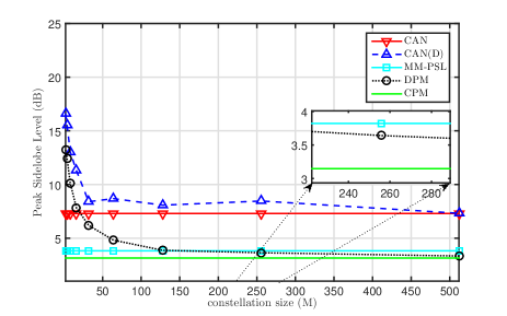
(a) PSL (dB) versus constellation size.

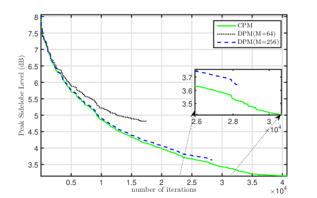
(b) PSL (dB) versus iteration.

Figure 1: The effects of constellation size on PSL values.

In Fig. 1.(b) the convergence behavior after heuristic initialization of CPM and DPM, for $M=64$ and $M=256$, is analyzed. As expected, the lower the alphabet size the faster the convergence but the worst the obtained PSL. Indeed, increasing $M$ (CPM is tantamount to considering $M=\infty$) the feasible set of DPM becomes larger and larger enabling better and better PSLs; nevertheless, more and more iterations are required to explore the enlarged domain. Finally, the convergence curves illustrate the monotonic decreasing behavior of the objective function.
The second experiment provides the PSL for sequence lengths $[5^{2},7^{2},10^{2},12^{2},15^{2},18^{2},20^{2},25^{2},30^{2},32^{2}]$. The results of CPM, DPM, CAN, and MM-PSL are shown in Fig. 2. The plot reveals that CPM exhibits a performance level better than the counterparts for all the considered lengths. Meanwhile, DPM with alphabet size $M=256$ obtains usually better PSL as compared with MM-PSL.

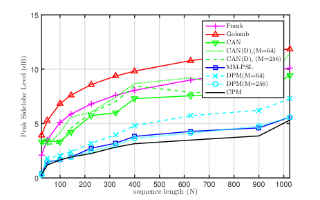
Figure 2: PSL (dB) versus sequence length.

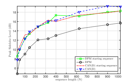
(a) $M=2$.

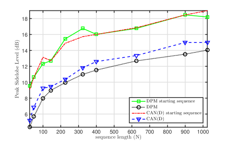
(b) $M=8$.

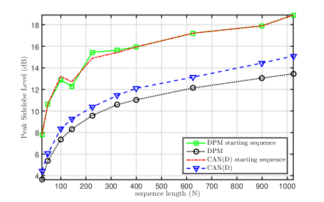
(c) $M=16$.

Figure 3: A comparison between CAN(D) and DPM starting from the same random sequence.

Next, the capability of DPM to design discrete phase sequences is assessed. In Fig. 3, the PSL versus the code length of CAN(D) and DPM are reported for alphabet sizes $M=2$, $M=8$, and $M=16$. For each $M$, the same set of $5$ random sequences (drawn by a uniform distribution over the set of the feasible sequences) is used to initialize both the algorithms. The results show that DPM outperforms CAN(D) significantly with maximum gains of 3.98 dB, 1.47 dB, and 1.65 dB for $M=2$, $M=8$, and $M=16$, respectively.
The case of binary phase sequence design is further investigated considering ITROX [15] (the only optimization-based algorithm currently available in the open literature that provides good binary phase sequences) as benchmark. Precisely, in Fig. 4.(a) the PSL versus $N$ is displayed for both ITROX and DPM where the same set of $5$ binary random codes is used for initialization. To highlight the quality of DPM algorithm also the PSL of MPS sequences, obtained via exhaustive search up to the length of $105$, is shown in this figure. The plot clearly illustrates the effectiveness of our approach. Indeed, DPM significantly outperforms ITROX and provides a PSL quite close to the global optimum of MPS sequences but with a much lower computational complexity and without restrictions to the maximum code length. This last feature is particularly appealing since the higher $N$ the higher the pulse compression. Interestingly, DPM provides in some circumstances the global optimal solution (see in Fig. 4 the points where DPM and MPS coincide). In this respect, in Fig. 4.(b) the autocorrelation function of a binary random sequence which leads to the Barker sequence of length $11$ though DPM is depicted (notice that 15% of the trials leads to this PSL value via DPM). As another example, in Fig. 4.(c) the autocorrelation function devised via DPM for sequence length $126$ is displayed. Remarkably, the PSL is equal to 8 (4% of the trials leads to this PSL value via DPM and only 10% is higher than or equal to 11) whereas the best PSL that [14] obtains for the same sequence length using genetic algorithms is $11$ which further confirms the effectiveness of the new framework.

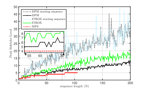
(a) A comparison among the PSL values of binary sequences obtained through DPM, ITROX-AP, and exhaustive search (MPS). For each length, DPM and ITROX-AP have been run 5 times and from the resulting 5 PSL values the best one is chosen.

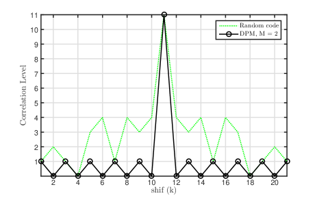
(b) Binary code design of length 11.

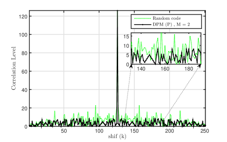
(c) Binary code design of length 126.

Figure 4: Performance of DPM algorithm in different conditions.

IV-B ISL Minimization

The performance assessment of CPM and DPM for ISL minimization is now considered. In this case, $\theta=0$ and the initialization procedure in Subsection III-C is not performed. In Fig. 5.(a), the ISL versus $M$ is displayed for DPM, CAN(D), CAN, WISL-Diag, and CPM assuming $N=400$. Interestingly, the continuous phase design strategies exhibit almost the same performance. As to the discrete phase code design, DPM outperforms the counterpart, i.e., CAN(D). Specifically, CAN(D) requires a larger constellation size than DPM to achieve the same ISL value. In Fig. 5.(b), the convergence behavior of CPM and DPM, for $M=64$ and $M=256$, is plotted and similar considerations to those for Fig. 1.(b) hold true.

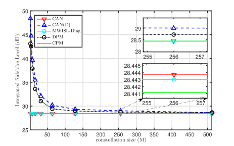
(a) ISL versus constellation size.

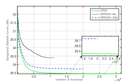
(b) Convergence curve for ISL minimization with $N=400$.

Figure 5: The effect of constellation size on ISL values.

To further corroborate the effectiveness of our strategies, in Fig. 6 the ISL versus $N$ is illustrated. In line with the previous results, the continuous phase design strategies are almost equivalent for all $N$ as well as DPM outperforms CAN(D).

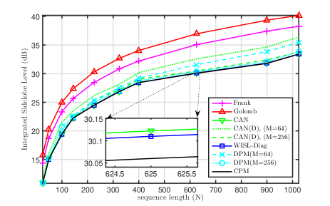
Figure 6: ISL (dB) versus sequence length.

Finally, Figs. 7.(a), 7.(b), and 7.(c) display the ISL versus $N$ for $M=2$, $M=8$, and $M=16$, respectively. $5$ random sequences (drawn by a uniform distribution over the set of the feasible sequences) are considered as starting points and the best resulting code is picked up. The results clearly show the significant performance gain granted by DPM. Specifically, for binary phase codes the maximum ISL gain of DPM with respect to CAN(D) is 5.99 dB, whereas for $M=8$ and $M=16$ the gains are 1.73 dB and 1.4 dB, respectively.

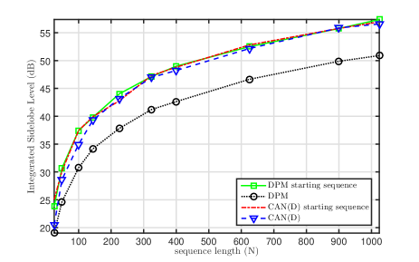
(a) ISL versus $N$ for binary phase sequence designed through CAN(D) and DPM.

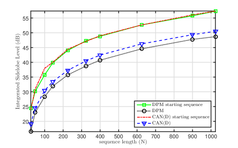
(b) ISL versus $N$ for discrete phase sequences with $M=8$ designed through CAN(D) and DPM.

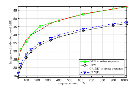
(c) ISL versus $N$ for discrete phase sequences with $M=16$ designed through CAN(D) and DPM.

Figure 7: ISL (dB) versus sequence length.

IV-C Pareto-Optimal Solution

In this subsection, the impact of the parameter $\theta$ on the designed codes is illustrated. Precisely, in Fig. 8 the Pareto curves obtained via CPM and DPM, for $M=64$ and $M=256$, are shown assuming $N=400$ and ${\theta}\in\{\theta_{1},\theta_{2},\ldots,\theta_{{6}}\}\subseteq[0,1]$, with $\theta_{i}=1-(i-1)/5$, $i=1,\ldots 6$. The starting sequence used at ${\theta}=\theta_{i}$ is the code optimized at ${\theta}=\theta_{i-1}$; also, at ${\theta}=\theta_{{1}}$ the heuristic approach of Subsection III-C is used. As expected, $\theta$ trades-off ISL and PSL values. Specifically, the higher $\theta$ the better the PSL and the worst the ISL, that is a classical feature of bi-objective Pareto curves. Otherwise stated, any solution is a Pareto optimal point.

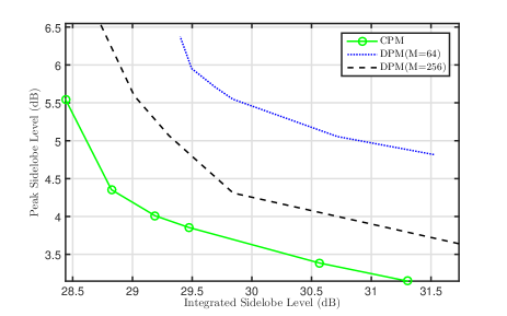
Figure 8: Pareto-optimal curves for continuous and discrete phases ($M=64$ and $M=256$) with $N=400$.

V Conclusion

The synthesis of phase sequences exhibiting good aperiodic correlation features has been addressed. Specifically, PSL and ISL have been adopted as performance metrics and the design problem has been formulated as a bi-objective optimization where either a continuous or a discrete phase constraint is imposed at the design stage. The non-convex and, in general, NP-hard problems resulting from scalarization are handled via a novel iterative procedure based on the CD method. Each iteration of the devised algorithm requires the solution of a non-convex min-max problem involving quartic functions. With reference to the continuous phase codes design, a new polynomial-time bisection method aimed at solving globally the aforementioned problem is developed. As to the discrete phase case, which includes the challenging and practically valuable binary codes synthesis, an FFT-based procedure is devised. Finally, some heuristic methods based $l_{p}$-norm minimization have been introduced to suitably initialize the new converge-ensured algorithms.

At the analysis stage, some interesting case studies have been provided to illustrate the effectiveness of the developed CD design approach. The results highlight the ability of the new procedures to design constant modulus sequences with enhanced autocorrelation properties. Precisely, the synthesized sequences grant better PSL and ISL than some counterparts available in the open literature. Besides, these gains are higher and higher as the constellation size reduces.

As future research tracks, it might be interesting to account for the behavior in the Doppler domain of the synthesized code, i.e., considering the design of codes with a proper ambiguity function, as well as consider a Peak to Average Ratio (PAR) constraint.

Appendix A Proof of Lemma III.1

Let,

$$|r_{k}(e^{\jmath\phi_{d}})|^{2} =\left|a_{dk}e^{\jmath\phi_{d}}+{b_{dk}e^{-\jmath\phi_{d}}+c_{dk}}\right|^{2}$$

$$=\bigg{|}\left(a_{dkr}e^{\jmath\phi_{d}}+b_{dkr}e^{-\jmath\phi_{d}}+c_{dkr}\right)$$

$$~{}~{}~{}~{}~{}~{}+\jmath\left(a_{dki}e^{\jmath\phi_{d}}+b_{dki}e^{-\jmath\phi_{d}}+c_{dki}\right)\bigg{|}^{2}$$

$$=\bigg{(}(a_{dkr}+b_{dkr})\cos(\phi_{d})$$

$$~{}~{}~{}~{}~{}~{}~{}~{}+(b_{dki}-a_{dki})\sin{(\phi_{d})}+c_{dkr}\bigg{)}^{2}$$

$$~{}~{}~{}+\bigg{(}(a_{dki}+b_{dki})\cos(\phi_{d})$$

$$~{}~{}~{}~{}~{}~{}~{}~{}+(a_{dkr}-b_{dkr})\sin{(\phi_{d})}+c_{dki}\bigg{)}^{2}$$

$$=A_{dk}+B_{dk}$$ (37)

where $a_{dkr}=\Re({a_{dk}})$, $b_{dkr}=\Re({b_{dk}})$, $c_{dkr}=\Re({c_{dk}})$, $a_{dki}=\Im({a_{dk}})$, $b_{dki}=\Im({b_{dk}})$ and $c_{dki}=\Im({c_{dk}})$. Also,

$$A_{dk}= \bigg{(}(a_{dkr}+b_{dkr})\cos(\phi_{d})$$ (38)

$$+(b_{dki}-a_{dki})\sin{(\phi_{d})}+c_{dkr}\bigg{)}^{2}$$

$$B_{dk}= \bigg{(}(a_{dki}+b_{dki})\cos(\phi_{d})$$ (39)

$$+(a_{dkr}-b_{dkr})\sin{(\phi_{d})}+c_{dki}\bigg{)}^{2}$$

Expanding (38)

$$A_{dk}= (a_{dkr}+b_{dkr})^{2}\cos^{2}(\phi_{d})$$ (40)

$$+2(a_{dkr}+b_{dkr})c_{dkr}\cos(\phi_{d})$$

$$+c_{dkr}^{2}+(b_{dki}-a_{dki})^{2}\sin^{2}(\phi_{d})$$

$$+2(a_{dkr}+b_{dkr})(b_{dki}-a_{dki})\sin(\phi_{d})\cos(\phi_{d})$$

$$+2c_{dkr}(b_{dki}-a_{dki})\sin(\phi_{d})$$

Hence, according to the trigonometric relationships [37, 38],

$$\sin{\phi_{d}} =\frac{2\tan\left({\frac{\phi_{d}}{2}}\right)}{1+\tan^{2}\left({\frac{\phi_{d}}{2}}\right)}$$ (41)

and

$$\cos{\phi_{d}} =\frac{1-2\tan^{2}\left({\frac{\phi_{d}}{2}}\right)}{1+\tan^{2}\left({\frac{\phi_{d}}{2}}\right)}$$ (42)

(40) can be recast as

$$A_{dk}= \frac{1}{(1+\beta_{d}^{2})^{2}}\{(a_{dkr}+b_{dkr})^{2}(1-\beta_{d}^{2})^{2}$$ (43)

$$+2(a_{dkr}+b_{dkr})c_{dkr}(1-\beta_{d}^{4})$$

$$+c_{dkr}^{2}(1+\beta_{d}^{2})^{2}+4\beta_{d}^{2}(b_{dki}-a_{dki})^{2}$$

$$+4\beta_{d}(1-\beta_{d}^{2})(a_{dkr}+b_{dkr})(b_{dki}-a_{dki})$$

$$+4\beta_{d}c_{dkr}(b_{dki}-a_{dki})$$

$$+4\beta_{d}^{3}c_{dkr}(b_{dki}-a_{dki})\}$$

with $\beta_{d}=\tan\left({\frac{\phi_{d}}{2}}\right)$. Besides, using standard algebra it is not difficult to show that,

$$A_{dk}=\frac{\mu^{\prime}_{dk}\beta_{d}^{4}+\kappa^{\prime}_{dk}\beta_{d}^{3}+\xi^{\prime}_{dk}\beta_{d}^{2}+\eta^{\prime}_{dk}\beta_{d}+\rho^{\prime}_{dk}}{(1+\beta_{d}^{2})^{2}}$$ (44)

with

$$\mu^{\prime}_{dk}= (a_{dkr}+b_{dkr})^{2}-2c_{dkr}(a_{dkr}+b_{dkr})+c_{dkr}^{2}$$

$$\kappa^{\prime}_{dk}= -4(a_{dkr}+b_{dkr})(b_{dki}-a_{dki})+4c_{dkr}(b_{dki}-a_{dki})$$

$$\xi^{\prime}_{dk}= -2(a_{dkr}+b_{dkr})^{2}+2c_{dkr}^{2}+4(b_{dki}-a_{dki})^{2}$$

$$\eta^{\prime}_{dk}= 4(a_{dkr}+b_{dkr})(b_{dki}-a_{dki})+4c_{dkr}(b_{dki}-a_{dki})$$

$$\rho^{\prime}_{dk}= (a_{dkr}+b_{dkr})^{2}+2(a_{dkr}+b_{dkr})c_{dkr}+c_{dkr}^{2}$$

A similar procedure on $B_{dk}$ yields,

$$B_{dk}=\frac{\mu^{\prime\prime}_{dk}\beta_{d}^{4}+\kappa^{\prime\prime}_{dk}\beta_{d}^{3}+\xi^{\prime\prime}_{dk}\beta_{d}^{2}+\eta^{\prime\prime}_{dk}\beta_{d}+\rho^{\prime\prime}_{dk}}{(1+\beta_{d}^{2})^{2}}$$ (45)

where

$$\mu^{\prime\prime}_{dk}= (a_{dki}+b_{dki})^{2}-2c_{dki}(a_{dki}+b_{dki})+c_{dki}^{2}$$

$$\kappa^{\prime\prime}_{dk}= -4(a_{dki}+b_{dki})(a_{dkr}-b_{dkr})+4c_{dki}(a_{dkr}-b_{dkr})$$

$$\xi^{\prime\prime}_{dk}= -2(a_{dki}+b_{dki})^{2}+2c_{dki}^{2}+4(a_{dkr}-b_{dkr})^{2}$$

$$\eta^{\prime\prime}_{dk}= 4(a_{dki}+b_{dki})(a_{dkr}-b_{dkr})+4c_{dki}(a_{dkr}-b_{dkr})$$

$$\rho^{\prime\prime}_{dk}= (a_{dki}+b_{dki})^{2}+2(a_{dki}+b_{dki})c_{dki}+c_{dki}^{2}$$

Finally,

$$|\widetilde{r}_{k}(\beta_{d})|^{2}=\frac{\mu_{dk}\beta_{d}^{4}+\kappa_{dk}\beta_{d}^{3}+\xi_{dk}\beta_{d}^{2}+\eta_{dk}\beta_{d}+\rho_{dk}}{(1+\beta_{d}^{2})^{2}}$$ (46)

where $\mu_{dk}=\mu^{\prime}_{dk}+\mu^{\prime\prime}_{dk}$, $\kappa_{dk}=\kappa^{\prime}_{dk}+\kappa^{\prime\prime}_{dk}$, $\xi_{dk}=\xi^{\prime}_{dk}+\xi^{\prime\prime}_{dk}$, $\eta_{dk}=\eta^{\prime}_{dk}+\eta^{\prime\prime}_{dk}$ and $\rho_{dk}=\rho^{\prime}_{dk}+\rho^{\prime\prime}_{dk}$.

Appendix B Derivation of the feasibility set

Let

$$\bar{p}(x)=ax^{4}+bx^{3}+cx^{2}+dx+e,$$ (47)

with $x,a,b,c,d,e\in\mathbb{R}$ as well as $[a,b,c,d,e]^{T}\neq{\bf 0}$, and let $\bar{p}^{{}^{\prime}}(x)$, $\bar{p}^{{}^{\prime\prime}}(x)$, $\bar{p}^{{}^{\prime\prime\prime}}(x)$, $\bar{p}^{(4)}(x)$ be the first order, second order, third order, and fourth order derivatives of $\bar{p}(x)$, respectively. Moreover, denote by $L\leq 4$ the number of distinct real roots of $\bar{p}(x)$ and let $x_{i}$, $i=1,\ldots,L$, be the ordered real roots. Since $\bar{p}^{(4)}(x)$ is a continuous function, the following steps allows to construct the set $\overline{\cal{A}}=\{x\,:\,\bar{p}(x)>0\}$:

• Let $\overline{\cal{A}}_{k}=\varnothing$;

• Find the real roots of $\bar{p}(x)$:

  • If $L=0$, then if the constant term $e\leq 0$ exit. Conversely, update $\overline{\cal{A}}_{k}=\mathbb{R}$ and exit;

  • If $L\geq 1$, sort the real roots, set $i=1$, and perform the remaining steps;

• If $\bar{p}^{{}^{\prime}}(x_{i})>0$, then $\bar{p}(x)>0$ on the interval ${(x_{i},x_{i+1})}$: update $\overline{\cal{A}}_{k}=\overline{\cal{A}}_{k}\cup(x_{i},x_{i+1})$; if $i<L$ set $i=i+1$ and repeat step [3], otherwise exit;

• If $\bar{p}^{{}^{\prime}}(x_{i})<0$, then $\bar{p}(x_{i})>0$ on the interval ${(x_{i-1},x_{i})}$: update $\overline{\cal{A}}_{k}=\overline{\cal{A}}_{k}\cup(x_{i-1},x_{i})$; if $i<L$ set $i=i+1$ and repeat step [3], otherwise exit;

• If $\bar{p}^{{}^{\prime}}(x_{i})=0$, then $x_{i}$ is a stationary point:

  • If $\bar{p}^{{}^{\prime\prime}}(x_{i})>0$, then $x_{i}$ is a local minimum: update $\overline{\cal{A}}_{k}=\overline{\cal{A}}_{k}\cup(x_{i-1},x_{i})\cup(x_{i},x_{i+1})$; if $i<L$ set $i=i+1$ and repeat step [3], otherwise exit;

  • If $\bar{p}^{{}^{\prime\prime}}(x_{i})<0$, then $x_{i}$ is a local maximum: if $i<L$ set $i=i+1$ and repeat step [3], otherwise exit;

  • If $\bar{p}^{{}^{\prime\prime}}(x_{i})=0$:

    • If $\bar{p}^{{}^{\prime\prime\prime}}(x_{i})\neq 0$, then $x_{i}$ is an inflection point. If $\bar{p}^{{}^{\prime\prime\prime}}(x_{i})>0$: update $\overline{\cal{A}}_{k}=\overline{\cal{A}}_{k}\cup(x_{i},x_{i+1})$; if $i<L$ set $i=i+1$ and repeat step [3], otherwise exit. Conversely if $\bar{p}^{{}^{\prime\prime\prime}}(x_{i})<0$: update $\overline{\cal{A}}_{k}=\overline{\cal{A}}_{k}\cup(x_{i-1},x_{i})$; if $i<L$ set $i=i+1$ and repeat step [3], otherwise exit;

    • If $\bar{p}^{{}^{\prime\prime\prime}}(x_{i})=0$,

      • If $\bar{p}^{(4)}(x_{i})>0$, then $x_{i}$ is a local minimum: update $\overline{\cal{A}}_{k}=\overline{\cal{A}}_{k}\cup(x_{i-1},x_{i})\cup(x_{i},x_{i+1})$; if $i<L$ set $i=i+1$ and repeat step [3], otherwise exit. Conversely, if $\bar{p}^{(4)}(x_{i})<0$ then $x_{i}$ is a local maximum: if $i<L$ set $i=i+1$ and repeat step [3], otherwise exit.

In order to calculate the union of the different sets, the fast and simple “union-find” algorithm [33] is employed. Precisely, let $(l_{1},u_{2}),(l_{2},u_{2}),\ldots,(l_{M},u_{M})$ be $M$ different intervals where $l_{i}$ is the lower bound of each set and $u_{i}$ is the upper bound. Let $\mbox{\boldmath{$t$}}\in{\cal{R}}^{M}$ be the vector containing the sorted $l_{i}$ and $u_{i}$, $i=1,\ldots,M$ in increasing order (if $l_{i}=u_{k}$ then $u_{k}$ is located first than $l_{i}$). Now, define a counter $Count$ initialized as $Count=1$; then check if the second entry of $t$ is a left extreme or a right extreme of one of $M$ intervals. If it is a left extreme, $Count=Count+1$ otherwise $Count=Count-1$. Now, if $Count=0$ an interval disjoint from the remaining part of the set is obtained and the process continues for the construction of the remaining part of the union set starting from the successive entry of $t$.

Appendix C Proof of Lemma III.2

The $M$-point DFT of $\mbox{\boldmath{$\zeta$}}_{dk}$ is,

$${\cal{F}}_{M}(\mbox{\boldmath{$\zeta$}}_{dk})=\left[\begin{array}[]{c}a_{dk}+c_{dk}+b_{dk}\\ a_{dk}+c_{dk}e^{-\jmath\frac{2\pi}{M}}+b_{dk}e^{-\jmath\frac{4\pi}{M}}\\ \vdots\\ a_{dk}+c_{dk}e^{-\jmath\frac{2\pi(M-1)}{M}}+b_{dk}e^{-\jmath\frac{4\pi(M-1)}{M}}\\ \end{array}\right]$$

Next, observe that

$${\widetilde{r}_{k}}(\bar{\phi_{m}})e^{-\jmath\bar{\phi_{m}}}=a_{dk}+c_{dk}e^{-\jmath\bar{\phi_{m}}}+b_{dk}e^{-2\jmath\bar{\phi_{m}}},~{}~{}~{}m=1,\ldots,M$$ (48)

Since $|{\widetilde{r}_{k}}(\bar{\phi_{m}})=e^{-\jmath\bar{\phi_{m}}}|=|{\widetilde{r}_{k}}(\bar{\phi_{m}})|$,

$$\left|{\cal{F}}_{M}(\mbox{\boldmath{$\zeta$}}_{dk})\right|=\left[|\widetilde{r}_{k}(\bar{\phi}_{1})|,|\widetilde{r}_{k}(\bar{\phi}_{2})|,\ldots,|\widetilde{r}_{k}(\bar{\phi}_{M})|\right]^{T}.$$ (49)

Appendix D Proof of Lemma III.3

Let

$$\Re\left\{r_{k}^{*}\frac{r_{k}^{(n)}}{\left|r_{k}^{(n)}\right|}\right\}= \Re\left\{\left[a_{dk}^{*}e^{-\jmath\phi_{d}}+{b_{dk}^{*}e^{\jmath\phi_{d}}+c_{dk}^{*}}\right]\frac{r_{k}^{(n)}}{\left|r_{k}^{(n)}\right|}\right\}$$ (50)

$$= \Re\left\{\widetilde{a}_{dk}e^{-\jmath\phi_{d}}+{\widetilde{b}_{dk}e^{\jmath\phi_{d}}+\widetilde{c}_{dk}}\right\}$$

$$= (\widetilde{a}_{dkr}+\widetilde{b}_{dkr})\cos(\phi_{d})$$

$$+(\widetilde{a}_{dki}-\widetilde{b}_{dki})\sin{(\phi_{d})}+\widetilde{c}_{dkr}$$

where $\widetilde{a}_{dkr}=\Re({a_{dk}^{*}\frac{r_{k}^{(n)}}{\left|r_{k}^{(n)}\right|}})$, $\widetilde{b}_{dkr}=\Re({b_{dk}^{*}\frac{r_{k}^{(n)}}{\left|r_{k}^{(n)}\right|}})$, $\widetilde{c}_{dkr}=\Re({c_{dk}^{*}\frac{r_{k}^{(n)}}{\left|r_{k}^{(n)}\right|}})$, $\widetilde{a}_{dki}=\Im({a_{dk}^{*}\frac{r_{k}^{(n)}}{\left|r_{k}^{(n)}\right|}})$ and $\widetilde{b}_{dki}=\Im({b_{dk}^{*}\frac{r_{k}^{(n)}}{\left|r_{k}^{(n)}\right|}})$.
As in Appendix A, using the change of variable $\cos{(\phi_{d})}=\frac{1-\beta_{d}^{2}}{1+\beta_{d}^{2}}$ and $\sin{(\phi_{d})}=\frac{2\beta_{d}}{1+\beta_{d}^{2}}$,

$$\Re\left\{r_{k}^{*}\frac{r_{k}^{(n)}}{\left|r_{k}^{(n)}\right|}\right\}= \frac{1}{(1+\beta_{d}^{2})^{2}}\{(\widetilde{a}_{dkr}+\widetilde{b}_{dkr})(1-\beta_{d}^{4})$$ (51)

$$+(\widetilde{a}_{dki}-\widetilde{b}_{dki})(2\beta_{d})(1+\beta_{d}^{2})$$

$$\widetilde{c}_{dkr}(1+\beta_{d}^{2})^{2}.\}$$

Finally, defining $\widetilde{\mu}_{dk}=\widetilde{c}_{dkr}-\widetilde{a}_{dkr}-\widetilde{b}_{dkr}$, $\widetilde{\kappa}_{dk}=2(\widetilde{a}_{dki}-\widetilde{b}_{dki})$, $\widetilde{\xi}_{dk}=2\widetilde{c}_{dkr}$, $\widetilde{\eta}_{dk}=2(\widetilde{a}_{dki}-\widetilde{b}_{dki})$ and $\widetilde{\rho}_{dk}=\widetilde{a}_{dkr}+\widetilde{b}_{dkr}+\widetilde{c}_{dkr}$ yields

$$\Re\left\{r_{k}^{*}\frac{r_{k}^{(n)}}{\left|r_{k}^{(n)}\right|}\right\}=\frac{\widetilde{\mu}_{dk}\beta_{d}^{4}+\widetilde{\kappa}_{dk}\beta_{d}^{3}+\widetilde{\xi}_{dk}\beta_{d}^{2}+\widetilde{\eta}_{dk}\beta_{d}+\widetilde{\rho}_{dk}}{(1+\beta_{d}^{2})^{2}}.$$

References

• [1] P. Woodward, Probability and Information Theory: With Applications to Radar. No. v. 3 in Electronics and Waves, Elsevier Science & Technology, 1953.
• [2] H. He, J. Li, and P. Stoica, Waveform Design for Active Sensing Systems. Cambridge University Press, 2012.
• [3] R. Barker, “Group synchronizing of binary digital systems,” Communication theory, pp. 273–287, 1953.
• [4] J. Kretschmer, F.F. and K. Gerlach, “Low sidelobe radar waveforms derived from orthogonal matrices,” IEEE Transactions on Aerospace and Electronic Systems, vol. 27, pp. 92–102, Jan 1991.
• [5] C. Nunn and G. Coxson, “Best-known autocorrelation peak sidelobe levels for binary codes of length 71 to 105,” IEEE Transactions on Aerospace and Electronic Systems, vol. 44, pp. 392–395, Jan 2008.
• [6] G. Stimson, H. Griffiths, H. Griffiths, D. Adamy, and C. Baker, Stimson’s Introduction to Airborne Radar. SciTech Publishing, Incorporated, 2014.
• [7] N. Levanon and E. Mozeson, Radar Signals. Wiley, 2004.
• [8] F. Gini, A. De Maio, and L. K. Patton, Waveform Design and Diversity for Advanced Radar Systems. The Institution of Engineering and Technology (IET), 2012.
• [9] H. He, P. Stoica, and J. Li, “Designing unimodular sequence sets with good correlations; including an application to MIMO radar,” IEEE Transactions on Signal Processing, vol. 57, pp. 4391–4405, Nov 2009.
• [10] M. M. Naghsh, M. Modarres-Hashemi, S. Shahbazpanahi, M. Soltanalian, and P. Stoica, “Unified optimization framework for multi-static radar code design using information-theoretic criteria,” IEEE Transactions on Signal Processing, vol. 61, pp. 5401–5416, Nov 2013.
• [11] M. M. Naghsh, M. Soltanalian, P. Stoica, M. Modarres-Hashemi, A. De Maio, and A. Aubry, “A Doppler robust design of transmit sequence and receive filter in the presence of signal-dependent interference,” IEEE Transactions on Signal Processing, vol. 62, pp. 772–785, Feb 2014.
• [12] J. Song, P. Babu, and D. P. Palomar, “Sequence design to minimize the weighted integrated and peak sidelobe levels,” IEEE Transactions on Signal Processing, vol. 64, pp. 2051–2064, Apr 2016.
• [13] M. Skolnik, Radar Handbook, Third Edition. Electronics electrical engineering, McGraw-Hill Education, 2008.
• [14] M. Nasrabadi and M. Bastani, A Survey on the Design of Binary Pulse Compression Codes with Low Autocorrelation. INTECH Open Access Publisher, 2010.
• [15] M. Soltanalian and P. Stoica, “Computational design of sequences with good correlation properties,” IEEE Transactions on Signal Processing, vol. 60, pp. 2180–2193, May 2012.
• [16] M. Friese, “Polyphase Barker sequences up to length 36,” IEEE Transactions on Information Theory, vol. 42, pp. 1248–1250, Jul 1996.
• [17] P. Borwein and R. Ferguson, “Polyphase sequences with low autocorrelation,” IEEE Transactions on Information Theory, vol. 51, pp. 1564–1567, Apr 2005.
• [18] C. Nunn, “Constrained optimization applied to pulse compression codes and filters,” in IEEE International Radar Conference, pp. 190–194, May 2005.
• [19] C. Nunn and G. Coxson, “Polyphase pulse compression codes with optimal peak and integrated sidelobes,” IEEE Transactions on Aerospace and Electronic Systems, vol. 45, pp. 775–781, Apr 2009.
• [20] J. Li, P. Stoica, and X. Zheng, “Signal synthesis and receiver design for MIMO radar imaging,” IEEE Transactions on Signal Processing, vol. 56, pp. 3959–3968, Aug 2008.
• [21] P. Stoica, H. He, and J. Li, “New algorithms for designing unimodular sequences with good correlation properties,” IEEE Transactions on Signal Processing, vol. 57, pp. 1415–1425, Apr 2009.
• [22] A. Aubry, A. De Maio, B. Jiang, and S. Zhang, “Ambiguity function shaping for cognitive radar via complex quartic optimization,” IEEE Transactions on Signal Processing, vol. 61, pp. 5603–5619, Nov 2013.
• [23] A. De Maio, Y. Huang, M. Piezzo, S. Zhang, and A. Farina, “Design of radar receive filters optimized according to $l_{p}$-norm based criteria,” IEEE Transactions on Signal Processing, vol. 59, pp. 4023–4029, Aug 2011.
• [24] B. Chen, S. He, Z. Li, and S. Zhang, “Maximum block improvement and polynomial optimization,” SIAM Journal on Optimization, vol. 22, pp. 87–107, Jan 2012.
• [25] K. Deb, Multi-objective optimization using evolutionary algorithms, vol. 16. John Wiley & Sons, 2001.
• [26] S. Boyd and L. Vandenberghe, Convex optimization. Cambridge university press, 2004.
• [27] A. De Maio, M. Piezzo, A. Farina, and M. Wicks, “Pareto-optimal radar waveform design,” Radar, Sonar & Navigation, IET, vol. 5, pp. 473–482, Apr 2011.
• [28] A. De Maio, M. Piezzo, S. Iommelli, and A. Farina, “Design of Pareto-optimal radar receive filters,” International Journal of Electronics and Telecommunications, vol. 57, no. 4, pp. 477–481, 2011.
• [29] S. J. Wright, “Coordinate descent algorithms,” Mathematical Programming, vol. 151, no. 1, pp. 3–34, 2015.
• [30] S. Buzzi, A. De Maio, and M. Lops, “Code-aided blind adaptive new user detection in DS/CDMA systems with fading time-dispersive channels,” IEEE Transactions on Signal Processing, vol. 51, pp. 2637–2649, Oct 2003.
• [31] P. Richtárik and M. Takáč, “Iteration complexity of randomized block-coordinate descent methods for minimizing a composite function,” Mathematical Programming, vol. 144, pp. 1–38, Jul 2014.
• [32] S. L. Shmakov, “A universal method of solving quartic equations,” International Journal of Pure and Applied Mathematics, vol. 71, pp. 251–259, Jun 2011.
• [33] R. Seidel and M. Sharir, “Top-down analysis of path compression,” SIAM Journal on Computing, vol. 34, pp. 515–525, Jul 2005.
• [34] S. G. Johnson and M. Frigo, “A modified split-radix FFT with fewer arithmetic operations,” IEEE Transactions on Signal Processing, vol. 55, pp. 111–119, Jan 2007.
• [35] J. Cilliers and J. Smit, “Pulse compression sidelobe reduction by minimization of $l_{p}$-norms,” IEEE Transactions on Aerospace and Electronic Systems, vol. 43, pp. 1238–1247, Jul 2007.
• [36] M. Razaviyayn, M. Hong, and Z.-Q. Luo, “A unified convergence analysis of block successive minimization methods for nonsmooth optimization,” SIAM Journal on Optimization, vol. 23, pp. 1126–1153, Sep 2013.
• [37] M. Abramowitz and I. A. Stegun, Handbook of mathematical functions: with formulas, graphs, and mathematical tables, vol. 55. Courier Corporation, 1964.
• [38] A. Ben-Tal and A. Nemirovski, Lectures on modern convex optimization: analysis, algorithms, and engineering applications, vol. 2. Siam, 2001.