Parallel Integer Polynomial Multiplication

Abstract

We propose a new algorithm for multiplying dense polynomials with integer coefficients in a parallel fashion, targeting multi-core processor architectures. Complexity estimates and experimental comparisons demonstrate the advantages of this new approach.

Keywords. Polynomial algebra; symbolic computation; parallel processing; cache complexity; multi-core architectures;

1 Introduction

Polynomial multiplication and matrix multiplication are at the core of many algorithms in symbolic computation. Expressing, in terms of multiplication time, the algebraic complexity of an operation, like univariate polynomial division or the computation of a characteristic polynomial, is a standard practice, see for instance the landmark book [36]. At the software level, the motto “reducing everything to multiplication” is also common, see for instance the computer algebra systems Magma [3], NTL [32] and FLINT [18].

With the advent of hardware accelerator technologies, such as multicore processors and Graphics Processing Units (GPUs), this reduction to multiplication is of course still desirable, but becomes more complex, since both algebraic complexity and parallelism need to be considered when selecting and implementing a multiplication algorithm. In fact, other performance factors, such as cache usage or CPU pipeline optimization, should be taken into account on modern computers, even on single-core processors. These observations guide the developers of projects like SPIRAL [29] or FFTW [11].

This paper is dedicated to the multiplication of dense univariate polynomials with integer coefficients targeting multicore processors. We note that the parallelization of sparse (both univariate and multivariate) polynomial multiplication on those architectures has already been studied by Gastineau & Laskar in [14], and by Monagan & Pearce in [25]. From now on, and throughout this paper, we focus on dense polynomials. The case of modular coefficients was handled in [26, 27] by techniques based on multi-dimensional FFTs. Considering now integer coefficients, one can reduce to the univariate situation through Kronecker’s substitution, see the implementation techniques proposed by Harvey in [19].

A first natural parallel solution for multiplying univariate integer polynomials is to consider divide-and-conquer algorithms where arithmetic counts are saved thanks to distributivity of multiplication over addition. Well-known instances of this solution are the multiplication algorithms of Toom & Cook, among which Karatsuba’s method is a special case. As we shall see with the experimental results of Section 4, this is a practical solution. However, the parallelism is limited by the number of ways in the recursion. Moreover, augmenting the number of ways increases data conversion costs and makes implementation quite complicated, see the work by Bodrato and Zanoni for the case of integer multiplication [2]. As in their work, our implementation includes the 4-way and 8-way cases. In addition, the algebraic complexity of an $N$-way Toom-Cook algorithm is not in the desirable complexity class of algorithms based on FFT techniques.

Turning our attention to this latter class, we first considered combining Kronecker’s substitution (so as to reduce multiplication in ${\mathbb{Z}}[x]$ to multiplication in ${\mathbb{Z}}$) and the algorithm of Schönhage & Strassen [31]. The GMP library [17] provides indeed a highly optimized implementation of this latter algorithm [15]. Despite of our efforts, we could not obtain much parallelism from the Kronecker substitution part of this approach. It became clear at this point that, in order to go beyond the performance (in terms of arithmetic count and parallelism) of our parallel $8$-way Toom-Cook code, our multiplication code had to rely on a parallel implementation of FFTs.

Based on the work of our colleagues from the SPIRAL and FFTW projects, and based on our experience on the subject of FFTs [26, 27, 24], we know that an efficient way to parallelize FFTs on multicore architectures is the so-called row-column algorithm [34]. which implies to view 1-D FFTs as multi-dimensional FFTs and thus differs from the approach of Schönhage & Strassen.

Reducing polynomial multiplication in ${\mathbb{Z}}[y]$ to multi-dimensional FFTs over a finite field, say ${\mathbb{Z}}/p{\mathbb{Z}}$, implies transforming integers to polynomials over ${\mathbb{Z}}/p{\mathbb{Z}}$. Chmielowiec in [6] experimented a similar method combined with the Chinese Remaindering Algorithm (CRA). However, as we shall see, using a big prime approach instead of a small primes approach opens the door for using “faster FFTs” and reducing algebraic complexity w.r.t to a CRA-based scheme.

As a result of all these considerations, we obtained the algorithm that we propose in this paper. We stress the fact that our purpose was not to design an algorithm asymptotically optimal by some complexity measures. Our purpose is to provide a parallel solution for dense integer polynomial multiplication on multicore architectures. In terms of algebraic complexity, our algorithm is asymptotically faster than that of Schönhage & Strassen [31] while being asymptotically slower than that of Fürer [13]. Our code is part of the Basic Polynomial Algebra Subprograms and is publicly available at http://www.bpaslib.org/.

Let $a(y),b(y)\in{\mathbb{Z}}[y]$ and $d$ be a positive integer such that $d-1$ is the maximum degree of $a$ and $b$, that is, $d={\max}({\deg}(a),{\deg}(b))+1$. We aim at computing the product $c(y):=a(y)$ $b(y)$. We propose an algorithm whose principle is sketched below. A precise statement of this algorithm is given in Section 2, while complexity results and experimental results appear in Sections 3 and 4.

Convert $a(y),b(y)$ to bivariate polynomials $A(x,y),B(x,$ $y)$ over ${\mathbb{Z}}$ (by converting the integer coefficients of $a(y),b(y)$ to univariate polynomials of ${\mathbb{Z}}[x]$, where $x$ is a new variable) such that $a(y)=A({\beta},y)$ and $b(y)=B({\beta},y)$ hold for some ${\beta}\in{\mathbb{Z}}$ (and, of course, such that we have ${\deg}(A,y)={\deg}(a)$ and ${\deg}(B,y)={\deg}(b)$).

Let $m>4H$ be an integer, where $H$ is the maximum absolute value of the coefficients of the integer polynomial $C(x,y):=A(x,y)B(x,y)$. The positive integers $m$, $K$ and the polynomials $A(x,y),B(x,y)$ are built such that the polynomials $C^{+}(x,y):=A(x,y)B(x,y)\mod{\langle x^{K}+1\rangle}$ and $C^{-}(x,y):=A(x,y)B(x,y)\mod{\langle x^{K}-1\rangle}$ are computed over ${\mathbb{Z}}/m{\mathbb{Z}}$ via FFT techniques, while the following equation holds over $\mathbb{Z}$:

$$C(x,y)\,=\,-\frac{C^{+}(x,y)}{2}(x^{K}-1)\,+\,\frac{C^{-}(x,y)}{2}(x^{K}+1).$$ (1)

Finally, one recovers the product $c(y)$ by evaluating the above equation at $x={\beta}$. Of course, the polynomials $A(x,y),B(x,y)$ are also constructed such that their total bit size is proportional to that of $a(y),b(y)$, respectively. In our software experimentation, this proportionality factor ranges between 2 and 4. Moreover, the number ${\beta}$ is a power of $2$ such that evaluating the polynomials $C^{+}(x,y)$ and $C^{-}(x,y)$ (whose coefficients are assumed to be in binary representation) at $x={\beta}$ amounts only to addition and shift operations.

Further, for our software implementation on 64-bit computer architectures, the number $m$ can be chosen to be either one machine word size prime $p$, a product $p_{1}p_{2}$ of two such primes or a product $p_{1}p_{2}p_{3}$ of three such primes. Therefore, in practice, the main arithmetic cost of the whole procedure is that of two, four or six convolutions, those latter being required for computing $C^{+}(x,y)$ and $C^{-}(x,y)$. All the other arithmetic operations (for constructing $A(x,y),B(x,y)$ or evaluating the polynomials $C^{+}(x,y)$ and $C^{-}(x,y)$) are performed in a single or double fixed precision at a cost which is proportional to that of reading/writing the byte vectors representing $A(x,y)$, $B(x,y)$, $C^{+}(x,y)$ and $C^{-}(x,y)$.

Theorem 1 below gives estimates for the work, the span and the cache complexity of the above algorithm. Recall that our goal is not to obtain an algorithm which is asymptotically optimal for one of these complexity measures. Instead, our algorithm is designed to be practically faster, on multi-core architectures, than the other algorithms that are usually implemented for the same purpose of multiplying dense (univariate) polynomials with integer coefficients.

Theorem 1

Let $N$ be a positive integer such that every coefficient of $a$ or $b$ can be written with at most $N$ bits. Let $K,M$ be two positive integers greater than 1 and such that $N=KM$. Assume that $K$ and $M$ are functions of $d$ satisfying the following asymptotic relations $K\in{\Theta}(d)$ and $M\in{\Theta}(\log{d})$. Then, the above algorithm for multiplying $a(y)$ and $b(y)$ has a work of $O(dKM{\log}(dK)\log\log(\log(d)))$ word operations, a span of $O({\log}_{2}(d)KM)$ word operations and incurs $O(1+(dMK/L)(1+{\log}_{Z}(dMK)))$ cache misses.

A detailed proof of this result is elaborated in Section 3. The assumptions $K\in{\Theta}(d)$ and $M\in{\Theta}(\log{d})$ are not strong. It is, indeed, possible to reduce to this situation by means of the balancing techniques presented in [27]. Applying those techniques would only increase the work by a constant multiplicative factor, typically between 2 and 4.

It follows from this result that our proposed algorithm is asymptotically faster than combining Kronecker’s substitution and Schönhage & Strassen. Indeed, with the notations of Theorem 1, this latter approach runs in $O(dN\log(dN)\log\log(dN))$ machine word operations.

While it is possible to obtain a poly-log time for the span this would correspond to an algorithm with high parallelism overheads. Hence, we prefer to state a bound corresponding to our implementation. By using multi-dimensional FFTs, we obtain a parallel algorithm which is practically efficient, as illustrated by the experimental results of Section 4. In particular, the algorithm scales well. In contrast, parallelizing a $k$-way Toom Cook algorithms (by executing concurrently the point-wise multiplication, see [22]) yields only a ratio work to span in the order of $k$, that is, a very limited scalability. Finally, our cache complexity estimate is sharp. Indeed, we control finely all intermediate steps with this respect, see Section 3.

To illustrate the benefits of a parallelized dense univariate polynomial multiplication, we integrated our code into the univariate real root isolation code presented in [5] together with a parallel version of Algorithm (E) from [35] for Taylor shifts. The results reported in [4] show that this integration has substantially improved the performance of our real root isolation code.

2 Multiplying integer polynomials via two convolutions

We write $a(y)=\sum_{i=0}^{d-1}\,a_{i}y^{i}$, $b(y)=\sum_{i=0}^{d-1}\,b_{i}y^{i}$ and $c(y)=\sum_{i=0}^{2d-2}\,c_{i}y^{i}$, where $a_{i},b_{i},c_{i}$ are integers and $c(y)=a(y)b(y)$. Let $N$ be a non-negative integer such that each coefficient ${\alpha}$ of $a$ or $b$ satisfies

$$-2^{N-1}\ \leq\ {\alpha}\ \leq\ 2^{N-1}-1$$ (2)

Therefore, using two’s complement, every such coefficient ${\alpha}$ can be encoded with $N$ bits. In addition, the integer $N$ is chosen such that $N$ writes

$$N=KM\ \ {\rm with}\ \ K\neq N\ \ {\rm and}\ \ M\neq N,$$ (3)

for $K,M\in{\mathbb{N}}$.

It is helpful to think of $M$ as a small number in comparison to $K$ and $d$, say that $M$ is in the order of the bit-size, called $w$, of a machine word. For the theoretical analysis of our algorithm, we shall assume, as in Theorem 1, that $K$ and $M$ are functions of $d$ satisfying $K\in{\Theta}(d)$ and $M\in\Theta(\log{d})$. We denote by $\mbox{{\sf DetermineBase}}(a,b,w)$ a function call returning $(N,K,M)$ satisfying those constraints as well as Relation (3).

Let $(N,K,M):=\mbox{{\sf DetermineBase}}(a,b,w)$ and define ${\beta}=2^{M}$. We write

$$a_{i}=\sum_{j=0}^{K-1}\,a_{i,j}{\beta}^{j},\ \ {\rm and}\ \ b_{i}=\sum_{j=0}^{K-1}\,b_{i,j}{\beta}^{j},$$ (4)

where each $a_{i,j}$ and $b_{i,j}$ are signed integers in the closed range $[-2^{M-1},2^{M-1}-1]$. Then, we define

$$A(x,y)=\sum_{i=0}^{d-1}\,(\sum_{j=0}^{K-1}\,a_{i,j}x^{j})y^{i},B(x,y)=\sum_{i=0}^{d-1}\,(\sum_{j=0}^{K-1}\,b_{i,j}x^{j})y^{i},$$ (5)

and

$$\begin{array}[]{l}C(x,y):=A(x,y)B(x,y)\ \ {\rm with}\\ C(x,y)=\sum_{i=0}^{2d-2}\,\left(\sum_{j=0}^{2K-2}\,c_{i,j}x^{j}\right)y^{i},\\ \end{array}$$ (6)

where $c_{i,j}\in{\mathbb{Z}}$. By ${\sf BivariateRepresentation}(a,N,K,M)$, we denote a function call returning $A(x,y)$ as defined above. Observe that the polynomial $c(y)$ is clearly recoverable from $C(x,y)$ by evaluating this latter polynomial at $x={\beta}$.

The following sequence of equalities will be useful:

$$\small\begin{array}[]{rl}C=&A\,B\\ =&\left(\sum_{i=0}^{d-1}\,(\sum_{j=0}^{K-1}\,a_{i,j}x^{j})y^{i}\right)\left(\sum_{i=0}^{d-1}\,(\sum_{j=0}^{K-1}\,b_{i,j}x^{j})y^{i}\right)\\ =&\sum_{i=0}^{2d-2}\left(\sum_{{\ell}+m=i}\left(\sum_{k=0}^{K-1}a_{{\ell},k}x^{k}\right)\left(\sum_{h=0}^{K-1}b_{m,h}x^{h}\right)\right)y^{i}\\ =&\sum_{i=0}^{2d-2}\left(\sum_{{\ell}+m=i}\left(\sum_{j=0}^{2K-2}\left(\sum_{k+h=j}a_{{\ell},k}b_{m,h}\right)x^{j}\right)\right)y^{i}\\ =&\sum_{i=0}^{2d-2}\left(\sum_{j=0}^{2K-2}c_{i,j}x^{j}\right)y^{i}\\ =&\sum_{j=0}^{2K-2}\left(\sum_{i=0}^{2d-2}c_{i,j}y^{i}\right)x^{j}\\ =&\sum_{j=0}^{K-1}\left(\sum_{i=0}^{2d-2}c_{i,j}y^{i}\right)x^{j}\\ &\ +\ x^{K}\sum_{j=0}^{K-2}\left(\sum_{i=0}^{2d-2}c_{i,j+K}\;y^{i}\right)x^{j},\\ \end{array}$$ (7)

where we have

$$c_{i,j}=\sum_{{\ell}+m=i}\sum_{k+h=j}a_{{\ell},k}b_{m,h},0\leq i\leq 2d-2,0\leq j\leq 2K-2,$$ (8)

with the convention

$$c_{i,2K-1}\ :=\ 0\ \ {\rm for}\ \ 0\leq i\leq 2d-2.$$ (9)

Since the modular products $A(x,y)B(x,y)\mod{\langle x^{K}+1\rangle}$ and $A(x,y)B(x,y)\mod{\langle x^{K}-1\rangle}$ are of interest, we define the bivariate polynomial over $\mathbb{Z}$

$$C^{+}(x,y)\ :=\ \sum_{i=0}^{2d-2}\,c^{+}_{i}(x)\,y^{i}\ \ {\rm where}\ \ c^{+}_{i}(x):=\sum_{j=0}^{K-1}\,c^{+}_{i,j}\,x^{j}$$ (10)

with $c^{+}_{i,j}:=c_{i,j}-c_{i,j+K}$, and the bivariate polynomial over $\mathbb{Z}$

$$C^{-}(x,y)\ :=\ \sum_{i=0}^{2d-2}\,c^{-}_{i}(x)\,y^{i}\ \ {\rm where}\ \ c^{-}_{i}(x):=\sum_{j=0}^{K-1}\,c^{-}_{i,j}\,x^{j}$$ (11)

with $c^{-}_{i,j}:=c_{i,j}+c_{i,j+K}.$ Thanks to Equation (7), we observe that we have

$$\begin{array}[]{rcl}C^{+}(x,y)&\equiv&A(x,y)B(x,y)\mod{\langle x^{K}+1\rangle},\\ C^{-}(x,y)&\equiv&A(x,y)B(x,y)\mod{\langle x^{K}-1\rangle}.\\ \end{array}$$ (12)

Since the polynomials $x^{K}+1$ and $x^{K}-1$ are coprime for the integer $K\geq 1$, we deduce Equation (1).

Since ${\beta}$ is a power of $2$, evaluating the polynomials $C^{+}(x,y)$, $C^{-}(x,y)$ and thus $C(x,y)$ (whose coefficients are assumed to be in binary representation) at $x={\beta}$ amounts only to addition and shift operations. A precise algorithm is described in Section 2.2. Before that, we turn our attention to computing $C^{+}(x,y)$ and $C^{-}(x,y)$ via FFT techniques.

2.1 Computing $C^{+}(x,y)$ and $C^{-}(x,y)$ via FFT

From Equation (12), it is natural to consider using FFT techniques for computing both $C^{+}(x,y)$ and $C^{-}(x,y)$. Thus, in order to compute over a finite ring supporting FFT, we estimate the size of the coefficients of $C^{+}(x,y)$ and $C^{-}(x,y)$. Recall that for $0\leq i\leq 2d-2$, we have

$$\begin{array}[]{rcll}c^{+}_{i,j}&=&c_{i,j}-c_{i,j+K}&\\ &=&\sum_{{\ell}+m=i}\sum_{k+h=j}a_{{\ell},k}b_{m,h}\\ &&-\sum_{{\ell}+m=i}\sum_{k+h=j+K}a_{{\ell},k}b_{m,h}.\\ \end{array}$$ (13)

Since each $a_{{\ell},k}$ and each $b_{m,h}$ has bit-size at most $M$, the absolute value of each coefficient $c^{+}_{i,j}$ is bounded over by $2\,d\,K\,2^{2M}$. The same holds for the coefficients $c^{-}_{i,j}$.

Since the coefficients $c^{+}_{i,j}$ and $c^{-}_{i,j}$ may be negative, we consider a prime number $p$ such that we have

$$p>4\,d\,K\,2^{2M}.$$ (14)

From now on, depending on the context, we freely view the coefficients $c^{+}_{i,j}$ and $c^{-}_{i,j}$ either as elements of $\mathbb{Z}$ or as elements of ${\mathbb{Z}}/p$. Indeed, the integer $p$ is large enough for this identification and we use the integer interval $[-\frac{p-1}{2},\frac{p-1}{2}]$ to represent the elements of ${\mathbb{Z}}/p$.

The fact that we follow a big prime approach, instead of an approach using machine word size primes and the Chinese Remaindering Algorithm, will be justified in Section 3.

A second requirement for the prime number $p$ is that the field ${\mathbb{Z}}/p$ should admit appropriate primitive roots of unity for computing the polynomials $C^{+}(x,y)$ and $C^{-}(x,y)$ via cyclic convolution and negacylic convolution as in Relation (12), that is, both $2d-1$ and $K$ must divide $p-1$. In view of utilizing 2-way FFTs, if $p$ writes $2^{k}q+1$ for an integer $q$, we must have:

$$(2d-1)\leq 2^{k}\ \ {\rm and}\ \ K\leq 2^{k}.$$ (15)

It is well-known that there are approximately $\frac{h}{2^{k-1}\,\log{(h)}}$ prime numbers $p$ of the form $2^{k}q+1$ for a positive integer $q$ and such that $p<h$ holds, see [36]. Hence, the number of prime numbers of the form $2^{k}q+1$ less than $2^{\ell}$ and greater than or equal to $2^{\ell-1}$ is approximately $\frac{2^{\ell-1}}{2^{k-1}\,{\ell}}$. For this latter fraction to be at least one, we must have

$$2^{{\ell}-\log_{2}({\ell})+1}\geq 2^{k}.$$

With (15) this yields:

$$2^{{\ell}-\log_{2}({\ell})+1}\geq(2d-1)\ \ {\rm and}\ \ 2^{{\ell}-\log_{2}({\ell})+1}\geq K,$$

from where we derive the following relation for choosing ${\ell}$:

$${\ell}-\log_{2}({\ell})\ \geq\ {\max}(\log_{2}(d),\log_{2}(K)).$$ (16)

We denote by ${\sf RecoveryPrime}(d,K,M)$ a function call returning a prime number $p$ satisfying Relation (14) and (16). Finally, we denote by $e$ the smallest number of $w$-bit words necessary to write $p$. Hence, we have

$$e\ \geq\ \left\lceil\frac{2+\lceil{\log}_{2}(d\,K)\rceil+2M}{w}\right\rceil.$$ (17)

Let ${\theta}$ be a $2K$-th primitive root of unity in ${\mathbb{Z}}/p$. We define $\omega={\theta}^{2}$; thus, $\omega$ is a $K$-th primitive root in ${\mathbb{Z}}/p$. For univariate polynomials $u(x),v(x)\in{\mathbb{Z}}[x]$ of degree at most $K-1$, computing $u(x)\,v(x)\mod{\langle x^{K}-1,p\rangle}$ via FFT is a well-known operation, see Algorithm 8.16 in [36]. Using the row-column algorithm for two-dimensional FFT, one can compute $C^{-}(x,y)\,\equiv\,A(x,y)B(x,y)\mod{\langle x^{K}-1,p\rangle}$, see [27, 26] for details. We denote by ${\sf CyclicConvolution}(A,B,K,p)$ the result of this calculation.

We turn our attention to the negacylic convolution, namely $A(x,y)B(x,y)\mod{\langle x^{K}+1,p\rangle}$. We observe that $C^{+}(x,y)\ \equiv\ A(x,y)B(x,y)\mod{\langle x^{K}+1,p\rangle}$ holds if only if $C^{+}({\theta}x,y)\ \equiv\ A({\theta}x,y)B({\theta}x,y)\mod{\langle x^{K}-1,p\rangle}$ does. Thus, defining $C^{\prime}(x,$ $y):=C^{+}({\theta}x,y)$, $A^{\prime}(x,y):=A({\theta}x,y)$ and $B^{\prime}(x,y):=B({\theta}x,y)$, we are led to compute $A^{\prime}(x,y)B^{\prime}(x,y)\mod{\langle x^{K}-1,p\rangle},$ which can be done as ${\sf CyclicConvolution}(A^{\prime},B^{\prime},K,p)$. Then, the polynomial $C^{+}(x,y)\mod{\langle x^{K}-1,p\rangle}$ is recovered from $C^{\prime}(x,y)\mod{\langle x^{K}-1,p\rangle}$ as

$$C^{+}(x,y)\ \equiv\ C^{\prime}({\theta}^{-1}x,y)\mod{\langle x^{K}-1,p\rangle},$$ (18)

and we denote by ${\sf NegacyclicConvolution}(A,B,K,p)$ the result of this process. We dedicate the following section to the final step of our algorithm, that is, the recovery of the product $c(y)$ from the polynomials $C^{+}(x,y)$ and $C^{-}(x,y)$.

2.2 Recovering $c(y)$ from $C^{+}(x,y)$ and $C^{-}(x,y)$

We naturally assume that all numerical coefficients are stored in binary representation. Thus, recovering $c(y)$ as $C({\beta},y)$ from Equation (1) involves only addition and shift operations. Indeed, ${\beta}$ is a power of $2$. Hence, the algebraic complexity of this recovery is essentially proportional to the sum of the bit sizes of $C^{+}(x,y)$ and $C^{-}(x,y)$. Therefore, the arithmetic count for computing these latter polynomials (by means of cyclic and negacyclic convolutions) dominates that of recovering $c(y)$. Nevertheless, when implemented on a modern computer hardware, this recovery step may contribute in a significant way to the total running time. The reasons are that: (1) both the convolution computation and recovery steps incur similar amounts of cache misses, and (2) the memory traffic implied by those cache misses is a significant portion of the total running time.

We denote by ${\sf RecoveringProduct}(C^{+}(x,y),C^{-}(x,y),{\beta})$ a function call recovering $c(y)$ from $C^{+}(x,y)$, $C^{-}(x,y)$ and ${\beta}=2^{M}$. We start by stating below a simple procedure for this operation:

$u(y)$ := $C^{+}({\beta},y)$,

$v(y)$ := $C^{-}({\beta},y)$,

$c(y)$ := $\frac{u(y)+v(y)}{2}+\frac{-u(y)+v(y)}{2}\,2^{N}$. To further describe this operation and, later on, in order to discuss its cache complexity and parallelization, we specify the data layout. From Relation (17), we can assume that each coefficient of the bivariate polynomials $C^{+}(x,y)$, $C^{-}(x,y)$ can be encoded within $e$ machine words. Thus, we assume that $C^{+}(x,y)$ (resp. $C^{-}(x,y)$) is represented by an array of $(2d-1)\,K\,e$ machine words such that, for $0\leq i\leq 2d-2$ and $0\leq j\leq K-1$, the coefficient $c^{+}_{i,j}$ (resp. $c^{-}_{i,j}$) is written between the positions $(K\,i+j)e$ and $(K\,i+j)e+e-1$, inclusively. Thus, this array can be regarded as the encoding of a 2-D matrix whose $i$-th row is $c^{+}_{i}(x)$ (resp. $c^{-}_{i}(x)$). Now, we write

$$u(y):=\sum_{i=0}^{2d-2}\,u_{i}y^{i}\ \ {\rm and}\ \ v(y):=\sum_{i=0}^{2d-2}\,v_{i}y^{i};$$ (19)

thus, from the definition of $u(y)$, $v(y)$, for $0\leq i\leq 2d-2$, we have

$$u_{i}=\sum_{j=0}^{K-1}\,c^{+}_{i,j}\,2^{M\,j}\ \ {\rm and}\ \ v_{i}=\sum_{j=0}^{K-1}\,c^{-}_{i,j}\,2^{M\,j}.$$ (20)

Denoting by $H^{+}$, $H^{-}$ the largest absolute value of a coefficient in $C^{+}(x,y)$, $C^{-}(x,y)$, we deduce

$$|u_{i}|\ \leq\ H^{+}{\frac{\left(\left({2}^{M}\right)^{K}-1\right)}{{2}^{M}-1}}\ \ {\rm and}\ \ |v_{i}|\ \leq\ H^{-}{\frac{\left(\left({2}^{M}\right)^{K}-1\right)}{{2}^{M}-1}}.$$ (21)

From the discussion justifying Relation (14), we have

$$H^{+},\,H^{-}\ \leq\ 2\,d\,K\,2^{2M},$$ (22)

and with (21) we derive

$$\begin{array}[]{rcl}|u_{i}|,\,|v_{i}|&\leq&2\,d\,K\,2^{M+N}.\\ \end{array}$$ (23)

Indeed, recall that $N=K\,M$ holds. We return to the question of data layout. Since each of $c^{+}_{i,j}$ or $c^{-}_{i,j}$ is a signed integer fitting within $e$ machine words, it follows from (21) that each of the coefficients $u_{i},v_{i}$ can be encoded within

$$f\ :=\ \lceil N/w\rceil+e$$ (24)

machine words. Hence, we store each of the polynomials $u(y),v(y)$ in an array of $(2d-1)\times f$ machine words such that the coefficient in degree $i$ is located between position $f\,i$ and position $f\,(i+1)-1$. Finally, we come to the computation of $c(y)$. We have

$$c_{i}\ =\ \frac{u_{i}+v_{i}}{2}\ +\ 2^{N}\ \frac{v_{i}-u_{i}}{2},$$ (25)

which implies

$$|c_{i}|\ \leq\ 2\,d\,K\,2^{M+N}(1+2^{N}).$$ (26)

Relation (26) implies that the polynomial $c(y)$ can be stored within an array of $(2d-1)\times 2f$ machine words. Of course, a better bound than (26) can be derived by simply expanding the product $a(y)\,b(y)$, leading to

$$|c_{i}|\ \leq\ d\,2^{2N-2}.$$ (27)

The ratio between the two bounds given by Relations (26) and (27) tells us that the extra amount of space required by our algorithm is $O({\log}_{2}(K)+M)$ bits per coefficient of $c(y)$. In practice, we aim at choosing $K,M$ such that $M\in{\Theta}({\log}_{2}(K))$, and if possible $M\leq w$. Hence, this extra space amount can be regarded as small and thus satisfactory.

2.3 The algorithm in pseudo-code

With the procedures that were defined in this section, we are ready to state our algorithm for integer polynomial multiplication.

Input: $a(y),b(y)\in{\mathbb{Z}}[y]$.

Output: the product $a(y)\,b(y)$

$(N,K,M)$ := ${\sf DetermineBase}(a(y),b(y),w)$

$A(x,y)$ := ${\sf BivariateRepresentation}(a(y),N,K,M)$

$B(x,y)$ := ${\sf BivariateRepresentation}(b(y),N,K,M)$

$p$ := ${\sf RecoveryPrime}(d,K,M)$

$C^{-}(x,y)$ := ${\sf CyclicConvolution}(A,B,K,p)$

$C^{+}(x,y)$ := ${\sf NegacyclicConvolution}(A,B,K,p)$

$c(y)$ := ${\sf RecoveringProduct}(C^{+}(x,y),C^{-}(x,y),2^{M})$

return $c(y)$

In order to analyze the complexity of our algorithm, it remains to specify the data layout for $a(y)$, $b(y)$, $A(x,y)$, $B(x,y)$. Note that this data layout question was handled for $C^{-}(x,y)$, $C^{+}(x,y)$ and $c(y)$ in Section 2.2.

In the sequel, we view $a(y)$, $b(y)$ as dense in the sense that each of their coefficients is assumed to be essentially of the same size. Hence, from the definition of $N$, see Relation (2), we assume that each of $a(y)$, $b(y)$ is stored within an array of $d\times\lceil N/w\rceil$ machine words such that the coefficient in degree $i$ is located between positions $\lceil N/w\rceil i$ and $\lceil N/w\rceil(i+1)-1$.

Finally, we assume that each of the bivariate integer polynomials $A(x,y)$, $B(x,y)$ is represented by an array of $d\times K$ machine words whose $(K\times i+j)$-th coefficient is $a_{i,j}$, $b_{i,j}$ respectively, for $0\leq i\leq d-1$ and $0\leq j\leq K-1$.

2.4 Parallelization

One of the initial motivations of our algorithm design is to take advantage of the parallel FFT-based routines for multiplying dense multivariate polynomials over finite fields that have been proposed in [26, 27]. To be precise, these routines provide us with a parallel implementation of the procedure CyclicConvolution, from which we easily derive a parallel implementation of NegacyclicConvolution.

Lines 1 and 4 can be ignored in the analysis of the algorithm. Indeed, one can simply implement DetermineBase and RecoveryPrimes by looking up in precomputed tables.

For parallelizing Lines 2 and 3, it is sufficient in practice to convert concurrently all the coefficients of $a(y)$ and $b(y)$ to univariate polynomials of ${\mathbb{Z}}[y]$. Similarly, for parallelizing Line 7, it is sufficient again to compute concurrently the coefficients of $u(y)$, $v(y)$ and then those of $c(y)$.

3 Complexity analysis

In this section, we analyze the algorithm stated in Section 2.3. We estimate its work and span as defined in the fork-join concurrency model  [1]. The reader unfamiliar with this model can regard the work as the time complexity on a multitape Turing machine [30] and the span as the minimum parallel running time of a “fork-join program”. Such programs use only two primitive language constructs, namely fork and join, in order to express concurrency. Since the fork-join model has no primitive constructs for defining parallel for-loops, each of those loops is simulated by a divide-and-conquer procedure for which non-terminal recursive calls are forked, see  [21] for details. Hence, in the fork-join model, the bit-wise comparison of two vectors of size $n$ has a span of $O({\log}(n))$ bit operations. This is actually the same time estimate as in the Exclusive-Read-Exclusive-Write PRAM [33, 16] model, but for a different reason.

We shall also estimate the cache complexity [12] of the serial counterpart of our algorithm for an ideal cache of $Z$ words and with $L$ words per cache line. The reader unfamiliar with this notion may understand it as a measure of memory traffic or, equivalently on multicore processors, as a measure of data communication. Moreover, the reader should note that the ratio work to cache complexity indicates how an algorithm is capable of re-using cached data. Hence, the larger is the ratio, the better the algorithm is.

We denote by $W_{i}$, $S_{i}$, $Q_{i}$ the work, span and cache complexity of Line ${\bf i}$ in the algorithm stated in Section 2.3. As mentioned before, we can ignore the costs of Lines 1 and 4. Moreover, we can use $W_{2}$, $S_{2}$, $Q_{2}$ as estimates for $W_{3}$, $S_{3}$, $Q_{3}$, respectively. Similarly, we can use the estimates of Line 5 for the costs of Line 6. Thus, we only analyze the costs of Lines 2, 5 and 7.

3.1 Choosing $K$, $M$ and $p$

In order to analyze the costs associated with the cyclic and negcyclic convolutions, we shall specify how $K$, $M$, $p$ are chosen. We shall assume thereafter that $K$ and $M$ are functions of $d$ satisfying the following asymptotic relations:

$$K\in{\Theta}(d)\ \ {\rm and}\ \ M\in{\Theta}(\log{d}).$$ (28)

It is a routine exercise to check that these assumptions together with Relation (14) imply Relation (16).

Relations (28) and (17) imply that we can choose $p$ and thus $e$ such that we have

$$e\in{\Theta}(\log{d}).$$ (29)

Here comes our most important assumption: one can choose $p$ and thus $e$ such that computing an FFT of a vector of size $s$ over ${\mathbb{Z}}/p[x]$, amounts to

$${\sf F}_{\rm arith}(e,s)\ \in\ O\left(s\frac{\log(s)}{\log(e)}\right)$$ (30)

arithmetic operations in ${\mathbb{Z}}/p$, whenever $e\in{\Theta}(\log{s})$ holds. Since each arithmetic operation in ${\mathbb{Z}}/p$ can be done within $O(e\log(e)\log\log(e))$ machine-word operations (using the multiplication algorithm of Schönhage and Strassen). Hence:

$${\sf F}_{\rm word}(e,s)\ \in\ O(s\,e\,\log(s)\,\log\log(e))$$ (31)

machine-word operations, whenever $e\in{\Theta}(\log{s})$ holds. Using the fork-join model, the corresponding span is $O(\log^{2}(s)\log^{2}(e)\log\log(e))$ machine-word operations.

Relation (30) can be derived from [8] assuming that $p$ is a generalized Fermat prime. Table 1 lists generalized Fermat primes of practical interest. Moreover, by adapting the results and proof strategy of [20] to the analysis in Section 2.6 of [7], we can obtain a similar binary complexity as that of Relation (30) for a prime $p$ which is not necessarily a generalized Fermat prime.

$p$	${\max}\{2^{k}\ {\rm s.t.}\ 2^{k}\,\mid\,p-1\}$
$(2^{63}+2^{53})^{2}+1$	$2^{106}$
$(2^{64}-2^{50})^{4}+1$	$2^{200}$
$(2^{63}+2^{34})^{8}+1$	$2^{272}$
$(2^{62}+2^{36})^{16}+1$	$2^{576}$
$(2^{62}+2^{56})^{32}+1$	$2^{1792}$
$(2^{63}-2^{40})^{64}+1$	$2^{2500}$
$(2^{64}-2^{28})^{128}+1$	$2^{3584}$

Table 1: Generalized Fermat primes of practical interest

3.2 Analysis of
${\sf BivariateRepresentation}(a(y),N,K,M)$

Converting each coefficient of $a(y)$ to a univariate polynomial of ${\mathbb{Z}}[x]$ requires $O(N)$ bit operations; thus,

$$W_{2}\in O(d\,N)\ \ {\rm and}\ \ S_{2}\in O({\log}(d)\,N).$$ (32)

The latter ${\log}(d)$ factor comes from the fact that the parallel for-loop corresponding to “for each coefficient of $a(y)$” is executed as a recursive function with $O({\log}(d))$ nested recursive calls. Considering the cache complexity and taking into account the data layout specified in Section 2.3, one can observe that converting $a(y)$ to $A(x,y)$ leads to $O(\lceil\frac{dN}{wL}\rceil+1)$ cache misses for reading $a(y)$ and $O(\lceil\frac{dKe}{L}\rceil+1)$ cache misses for writing $A(x,y)$. Therefore, we have:

$$Q_{2}\in O\left(\left\lceil\frac{dN}{wL}\right\rceil+\left\lceil\frac{dK\log_{2}(dK)}{wL}\right\rceil+1\right).$$ (33)

3.3 Analysis of ${\sf CyclicConvolution}(A,B,K,p)$

Following the techniques developed in [26, 27], we compute $A(x,y)B(x,y)\mod{\langle x^{K}-1,p\rangle}$ by 2-D FFT of format $K\times 2d$. In the direction of $y$, we need to do $K$ FFTs of size $2d$ leading to $O(K\,F_{\rm word}(e,2d))$ machine word operations. In the direction of $x$, we need to compute $2d$ convolutions (i.e. products in ${\mathbb{Z}}[x]/\langle x^{K}-1,p\rangle$) leading to $O(2d\,F_{\rm word}(e,K))$ machine word operations. Using Relations (28), (29) and (31), the work of one 2-D FFT of format $K\times 2d$ amounts to:

$$\begin{array}[]{rl}O(KF_{\rm word}(e,2d))+O(2dF_{\rm word}(e,K))&=\\ O(Ke2d(\log(2d)+\log(K))\log\log(e))&=\\ O(Ke2d\log(2dK)\log\log(e))&=\\ O(KM2d\log(2dK)\log\log(\log(d)))\end{array}$$ (34)

machine word operations, while the span amounts to:

$$\begin{array}[]{l}O((\log(K)\log^{2}(d)+\log(d)\log^{2}(K))\log^{2}(e)\log\log(e))\\ =O(\log(K)\log(d)\log(dK)\log^{2}(\log(d))\log\log(\log(d))).\end{array}$$ (35)

Hence:

$$W_{5}\in O(dKM{\log}(dK)\log\log(\log(d)))\ \ {\rm and}\ \$$ (36)

$S_{5}\in O(\log(K)\log(d)\log(dK)\log^{2}(\log(d))\log\log(\log(d)))$ machine word operations. Finally, from the results of [12] and assuming that $Z$ is large enough to accommodate a few elements of ${\mathbb{Z}}/p$, we have

$$Q_{6}\in O(1+(deK/L)(1+{\log}_{Z}(deK))).$$ (37)

3.4 Analysis of
${\sf RecoveringProduct}(C^{+}(x,y),C^{-}(x,y),2^{M})$

Converting each coefficient of $u(y)$ and $v(y)$ from the corresponding coefficients of $C^{+}(x,y)$ and $C^{-}(x,y)$ requires $O(K\,e)$ bit operations. Then, computing each coefficient of $c(y)$ requires $O(N+e\,w)$ bit operations. Thus, we have

$$W_{7}\in O(d\,(K\,e+N+e))\ \ {\rm and}\ \ S_{7}\in O({\log}(d)\,(K\,e+N+e))$$ (38)

word operations. Converting $C^{+}(x,y)$, $C^{-}(x,y)$ to $u(y)$, $v(y)$ leads to $O(\lceil d\,K\,e/L\rceil+1)$ cache misses for reading $C^{+}(x,y)$, $C^{-}(x,y)$ and $O(\lceil d(N/w+e)/L\rceil+1)$ cache misses for writing $u(y)$, $v(y)$. This second estimate holds also for the total number of cache misses for computing $c(y)$ from $u(y)$, $v(y)$. Thus, we have $Q_{7}\in O(\lceil d\,(K\,e+N+e)/L\rceil+1).$ We note that the quantity $K\,e+N+e$ can be replaced in above asymptotic upper bounds by $K({\log}_{2}(d\,K)+3\,M)$.

3.5 Proof of Theorem 1

Recall that analyzing our algorithm reduces to analyzing Lines 2, 5, 7. Based on the results obtained above for $W_{2}$, $W_{5}$, $W_{7}$, with Relations (32), (36), (38), respectively, it follows that the estimate for the work of the whole algorithm is given by $W_{5}$, leading to the result in Theorem 1. Meanwhile, the span of the whole algorithm is dominated by $S_{7}$ and one obtains the result in Theorem 1. Finally, the cache complexity estimate in Theorem 1 comes from adding up $Q_{2}$, $Q_{5}$, $Q_{7}$ and simplifying.

4 Experimentation

We realized an implementation of a modified version of the algorithm presented in Section 2. The only modification is that we rely on prime numbers $p$ that do not satisfy Equation (31). In particular, our implementation is not using yet generalized Fermat primes. Overcoming this limitation is work in progress. Currently, our prime numbers are of machine word size. As a consequence, the work of the implemented algorithm is $O(dKM{\log}(dK)({\log}(dK)+2M))$, which is asymptotically larger than the work of the approach combining Kronecker’s substitution and Schönhage & Strassen. This helps understanding why the speedup factor of our parallel implementation over the integer polynomial multiplication code of FLINT (which is a serial implementation of the algorithm of Schönhage & Strassen) is less than the number of cores that we use.

However, this latter complexity estimate yields a (modest) optimization trick: since the asymptotic upper bound $O(dKM{\log}(dK)({\log}(dK)+2M))$ increases slower with $M$ than with $d$ or $K$, it is advantageous to make $M$ large. We do that by using two machine word primes (and the Chinese Remaindering Algorithm) instead of using a single prime for computing two modular images of $C^{+}({x,y})$ and $C^{-}({x,y})$ that we combine by the Chinese Remaindering Algorithm. Moreover, our parallel implementation outperforms the integer polynomial multiplication code of Maple 2015.

Our code is written in the multi-threaded language CilkPlus [21] and compiled with the CilkPlus branch of GCC. Our experimental results were obtained on a 48-core AMD Opteron 6168, running at 900MHz with 256 GB of RAM and 512KB of L2 cache. Table 2 gives running times for the five multiplication algorithms that we have implemented:

${\rm KS}_{s}$ stands for Kronecker’s substitution combined with Schönhage & Strassen algorithm [31]; note this is a serial implementation, running on 1 core.

${\rm CVL}_{p}^{2}$ is the prototype implementation of the modified version of the algorithm described in Section 2, running on 48 cores. In this implementation, two machine-word size Fourier primes are used instead of a single big prime for computing $C^{+}({x,y})$ and $C^{-}({x,y})$.

${\rm DnC}_{p}$ is a straightforward 4-way divide-and-conquer parallel implementation of plain multiplication, run on 48 cores, see Chapter 2 of [22].

${\rm Toom}^{4}_{p}$ is a parallel implementation of 4-way Toom-Cook, run on 48 cores, see Chapter 2 of [22].

${\rm Toom}^{8}_{p}$ is a parallel implementation of 8-way Toom-Cook, run on 48 cores, see Chapter 2 of [22]. In Table 2, for each example, the degree $d$ of the input polynomial is equal to the coefficient bit size $N$. The input polynomials $a(y),b(y)$ are random and dense.

Figure 1 shows the running time comparison among our algorithm, FLINT 2.4.3 [18] and Maple 2015. The input of each test case is a pair of polynomials of degree $d$ where each coefficient has bit size $N$. Timings (in sec.) appear along the vertical axis. Two plots are provided: one for which $d=N$ holds and one for $d$ is much smaller than $N$.

From Table 2 and Figure 1, we observe that our implementation ${\rm CVL}_{p}^{2}$ performs better on sufficiently large input data, compared to its counterparts.

$d,N$	${\rm CVL}_{p}^{2}$	${\rm DnC}_{p}$	${\rm Toom}^{4}_{p}$	${\rm Toom}^{8}_{p}$	${\rm KS}_{s}$
$2^{9}$	0.152	0.049	0.022	0.026	0.018
$2^{10}$	0.139	0.11	0.046	0.059	0.057
$2^{11}$	0.196	0.17	0.17	0.17	0.25
$2^{12}$	0.295	0.58	0.67	0.64	1.37
$2^{13}$	0.699	2.20	2.79	2.73	5.40
$2^{14}$	1.927	8.26	10.29	8.74	20.95
$2^{15}$	9.138	30.75	35.79	33.40	92.03
$2^{16}$	33.04	122.1	129.4	115.9	*Err.

Table 2: Timings of polynomial multiplication with $d=N$

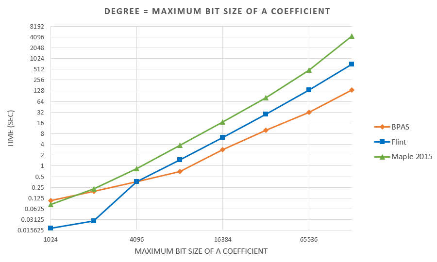
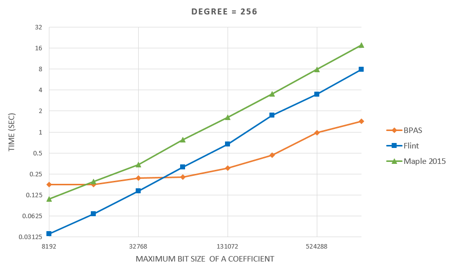
Figure 1: Dense integer polynomial multiplication: ${\rm CVL}_{p}^{2}$ (BPAS) vs FLINT vs Maple 2015

5 Concluding Remarks

We have presented a parallel FFT-based method for multiplying dense univariate polynomials with integer coefficients. Our approach relies on two convolutions (cyclic and negacyclic) of bivariate polynomials which allow us to take advantage of the row-column algorithm for 2D FFTs. The proposed algorithm is asymptotically faster than that of Schönhage & Strassen.

In our implementation, the data conversions between univariate polynomials over $\mathbb{Z}$ and bivariate polynomials over ${\mathbb{Z}}/p{\mathbb{Z}}$ are highly optimized by means of low-level “bit hacks” thus avoiding software multiplication of large integers. In fact, our code relies only and directly on machine word operations (addition, shift and multiplication).

Our experimental results show this new algorithm has a high parallelism and scales better than its competitor algorithms. Nevertheless, there is still room for improvement in the implementation. Using a single big prime (instead of two machine-word size primes and the Chinese Remaindering Algorithm), and requiring that this prime be a generalized Fermat prime, would make the implemented algorithm follow strictly that presented in Section 2.

References

- [1] R. D. Blumofe and C. E. Leiserson. Space-efficient scheduling of multithreaded computations. SIAM J. Comput., 27(1):202–229, 1998.
- [2] M. Bodrato and A. Zanoni. Integer and polynomial multiplication: towards optimal Toom-Cook matrices. In ISSAC, pages 17–24, 2007.
- [3] W. Bosma, J. Cannon, and C. Playoust. The Magma algebra system. I. The user language. J. Symbolic Comput., 24(3-4):235–265, 1997.
- [4] C. Chen, S. Covanov, F. Mansouri, M. Moreno Maza, N. Xie, and Y. Xie. The basic polynomial algebra subprograms. In International Congress on Mathematical Software, pages 669–676. Springer, 2014.
- [5] C. Chen, M. Moreno Maza, and Y. Xie. Cache complexity and multicore implementation for univariate real root isolation. J. of Physics: Conference Series, 341, 2011.
- [6] A. Chmielowiec. Parallel algorithm for multiplying integer polynomials and integers. In IAENG Transactions on Engineering Technologies, volume 229 of Lecture Notes in Electrical Engineering, pages 605–616. Springer, 2013.
- [7] S. Covanov and M. Moreno Maza. Putting Fürer algorithm into practice. Technical report, 2014. http://www.csd.uwo.ca/~moreno//Publications/Svyatoslav-Covanov-Rapport-de-Stage-Recherche-2014.pdf.
- [8] S. Covanov and E. Thomé. Fast integer multiplication using generalized Fermat primes. Jan. 2016. working paper or preprint.
- [9] A. De, P. P. Kurur, C. Saha, and R. Saptharishi. Fast integer multiplication using modular arithmetic. In C. Dwork, editor, STOC, pages 499–506. ACM, 2008.
- [10] A. De, P. P. Kurur, C. Saha, and R. Saptharishi. Fast integer multiplication using modular arithmetic. SIAM J. Comput., 42(2):685–699, 2013.
- [11] M. Frigo and S. G. Johnson. The design and implementation of FFTW3. Proceedings of the IEEE, 93(2):216–231, 2005.
- [12] M. Frigo, C. E. Leiserson, H. Prokop, and S. Ramachandran. Cache-oblivious algorithms. ACM Transactions on Algorithms, 8(1):4, 2012.
- [13] M. Fürer. Faster integer multiplication. SIAM J. Comput., 39(3):979–1005, 2009.
- [14] M. Gastineau and J. Laskar. Highly scalable multiplication for distributed sparse multivariate polynomials on many-core systems. In CASC, pages 100–115, 2013.
- [15] P. Gaudry, A. Kruppa, and P. Zimmermann. A GMP-based implementation of Schönhage-Strassen’s large integer multiplication algorithm. In ISSAC, pages 167–174, 2007.
- [16] P. B. Gibbons. A more practical PRAM model. In Proc. of SPAA, pages 158–168, 1989.
- [17] T. Granlund et al. GNU MP 6.0 Multiple Precision Arithmetic Library. Samurai Media Limited, 2015.
- [18] W. Hart, F. Johansson, and S. Pancratz. FLINT: Fast Library for Number Theory. V. 2.4.3, http://flintlib.org.
- [19] D. Harvey. Faster polynomial multiplication via multipoint Kronecker substitution. J. Symb. Comput., 44(10):1502–1510, 2009.
- [20] D. Harvey, J. van der Hoeven, and G. Lecerf. Even faster integer multiplication. Journal of Complexity, pages –, 2016.
- [21] C. E. Leiserson. The Cilk++ concurrency platform. The Journal of Supercomputing, 51(3):244–257, 2010.
- [22] F. Mansouri. On the parallelization of integer polynomial multiplication. Master’s thesis, The University of Western Ontario, London, ON, Canada, 2014. www.csd.uwo.ca/~moreno/Publications/farnam-thesis.pdf.
- [23] L. Meng and J. R. Johnson. Automatic parallel library generation for general-size modular FFT algorithms. In CASC, pages 243–256, 2013.
- [24] L. Meng, Y. Voronenko, J. R. Johnson, M. Moreno Maza, F. Franchetti, and Y. Xie. Spiral-generated modular FFT algorithms. In PASCO, pages 169–170, 2010.
- [25] M. B. Monagan and R. Pearce. Parallel sparse polynomial multiplication using heaps. In ISSAC, pages 263–270, 2009.
- [26] M. Moreno Maza and Y. Xie. FFT-based dense polynomial arithmetic on multi-cores. In HPCS, volume 5976 of Lecture Notes in Computer Science, pages 378–399. Springer, 2009.
- [27] M. Moreno Maza and Y. Xie. Balanced dense polynomial multiplication on multi-cores. Int. J. Found. Comput. Sci., 22(5):1035–1055, 2011.
- [28] A. Pospelov. Faster polynomial multiplication via discrete Fourier transforms. In A. S. Kulikov and N. K. Vereshchagin, editors, CSR, volume 6651 of Lecture Notes in Computer Science, pages 91–104. Springer, 2011.
- [29] M. Püschel, J. M. F. Moura, J. Johnson, D. Padua, M. Veloso, B. Singer, J. Xiong, F. Franchetti, A. Gacic, Y. Voronenko, K. Chen, R. W. Johnson, and N. Rizzolo. SPIRAL: Code generation for DSP transforms. Proceedings of the IEEE, special issue on “Program Generation, Optimization, and Adaptation”, 93(2):232– 275, 2005.
- [30] A. Schönhage, A. F. Grotefeld, and E. Vetter. Fast algorithms - a multitape Turing machine implementation. BI-Wissenschaftsverlag, 1994.
- [31] A. Schönhage and V. Strassen. Schnelle multiplikation großer zahlen. Computing, 7(3-4):281–292, 1971.
- [32] V. Shoup et al. NTL: A library for doing number theory. www.shoup.net/ntl/.
- [33] L. J. Stockmeyer and U. Vishkin. Simulation of parallel random access machines by circuits. SIAM J. Comput., 13(2):409–422, 1984.
- [34] C. Van Loan. Computational Frameworks for the Fast Fourier Transform. Society for Industrial and Applied Mathematics, Philadelphia, PA, USA, 1992.
- [35] J. von zur Gathen and J. Gerhard. Fast algorithms for Taylor shifts and certain difference equations. In ISSAC, pages 40–47, 1997.
- [36] J. von zur Gathen and J. Gerhard. Modern Computer Algebra. Cambridge University Press, NY, USA, 2 edition, 2003.