High order numerical schemes for one-dimension non-local conservation laws

Abstract.

This paper focuses on the numerical approximation of the solutions of non-local conservation laws in one space dimension. These equations are motivated by two distinct applications, namely a traffic flow model in which the mean velocity depends on a weighted mean of the downstream traffic density, and a sedimentation model where either the solid phase velocity or the solid-fluid relative velocity depends on the concentration in a neighborhood. In both models, the velocity is a function of a convolution product between the unknown and a kernel function with compact support. It turns out that the solutions of such equations may exhibit oscillations that are very difficult to approximate using classical first-order numerical schemes. We propose to design Discontinuous Galerkin (DG) schemes and Finite Volume WENO (FV-WENO) schemes to obtain high-order approximations. As we will see, the DG schemes give the best numerical results but their CFL condition is very restrictive. On the contrary, FV-WENO schemes can be used with larger time steps. We will see that the evaluation of the convolution terms necessitates the use of quadratic polynomials reconstructions in each cell in order to obtain the high-order accuracy with the FV-WENO approach. Simulations using DG and FV-WENO schemes are presented for both applications.

1. Introduction

This paper is concerned with the design of numerical schemes for the one-dimensional Cauchy problem for non-local scalar conservation law of the form

$$\begin{cases}\rho_{t}+(f(\rho)V(\rho*\omega_{\eta}))_{x}=0,&x\in\mathbb{R},\quad t>0,\\ \rho(x,0)=\rho_{0}(x)&x\in\mathbb{R},\end{cases}$$ (1.1)

where the unknown density $\rho$ depends on the space variable $x$ and the time variable $t$, $\rho\to V(\rho)$ is a given velocity function, and $\rho\to g(\rho)=f(\rho)V(\rho)$ is the usual flux function for the corresponding local scalar conservation law. Here, (1.1) is non-local in the sense that the velocity function $V$ is evaluated on a “neighborhood” of $x\in\mathbb{R}$ defined by the convolution of the density $\rho$ and a given kernel function $\omega_{\eta}$ with compact support. In this paper, we are especially interested in two specific forms of (1.1) which naturally arise in traffic flow modelling [9, 17] and sedimentation problems [8]. They are given as follows.
 
A non-local traffic flow model. In this context, we follow [9, 17] and consider (1.1) as an extension of the classical Lighthill-Whitham-Richards traffic flow model, in which the mean velocity is assumed to be a non-increasing function of the downstream traffic density and where the flux function is given by

$$f(\rho)=\rho,\quad V(\rho)={\color[rgb]{0,0,0}1-\rho},\quad(\rho*\omega_{\eta})(x,t)=\int_{x}^{x+\eta}\omega_{\eta}(y-x)\rho(y,t)dy.$$ (1.2)

Four different nonnegative kernel functions will be considered in the numerical section, namely $\omega_{\eta}(x)=1/\eta$, $\omega_{\eta}(x)=2(\eta-x)/\eta^{2}$, $\omega_{\eta}(x)=3(\eta^{2}-x^{2})/(2\eta^{3})$ and $\omega_{\eta}(x)=2x/\eta^{2}$ with support on $[0,\eta]$ for a given value of the real number $\eta>0$. Notice that the well-posedness of this model together with the design of a first and a second order FV approximation have been considered in [9, 17].
 
A non-local sedimentation model. Following [8], we consider under idealized assumptions that equation (1.1) represents a one-dimensional model for the sedimentation of small equal-sized spherical solid particles dispersed in a viscous fluid, where the local solids column fraction $\rho=\rho(x,t)$ is a function of depth $x$ and time $t$. In this context, the flux function is given by

$$f(\rho)=\rho(1-\rho)^{\alpha},\quad V(\rho)=(1-\rho)^{n},\quad(\rho*\omega_{\eta})(x,t)=\int_{-2\eta}^{2\eta}\omega_{\eta}(y)\rho(x+y,t)dy,$$ (1.3)

where $n\geq 1$ and the parameter $\alpha$ satisfies $\alpha=0$ or $\alpha\geq 1$. The function $V$ is the so-called hindered settling factor and the convolution term $\rho*\omega_{\eta}$ is defined by a symmetric, nonnegative, and piecewise smooth kernel function $\omega_{\eta}$ with support on $[-2\eta,2\eta]$ for a parameter $\eta>0$ and $\int_{\mathbb{R}}\omega_{\eta}(x)dx=1$. More precisely, the authors define in [8] a truncated parabola $K$ by

$$K(x)=\frac{3}{8}\left(1-\frac{x^{2}}{4}\right)\,\text{ for }|x|<2,\qquad K(x)=0\,\,\text{ otherwise, }$$

and set

$$\omega_{\eta}(x):=\eta^{-1}K(\eta^{-1}x).$$ (1.4)

Conservation laws with non-local terms arise in a variety of physical and engineering applications: besides the above cited ones, we mention models for granular flows [4], production networks [21], conveyor belts [18], weakly coupled oscillators [3], laser cutting processes [15], biological applications like structured populations dynamics [23], crowd dynamics [10, 12] or more general problems like gradient constrained equations [6].
While several analytical results on non-local conservation laws can be found in the recent literature (we refer to [7] for scalar equations in one space dimension, [5, 13, 24] for scalar equations in several space dimensions and [2, 14, 16] for multi-dimensional systems of conservation laws), few specific numerical methods have been developed up to now. Finite volume numerical methods have been studied in [2, 17, 22, 25]. At this regard, it is important to notice that the lack of Riemann solvers for non-local equations limits strongly the choice of the scheme. At the best of our knowledge, two main approaches have been proposed in the literature to treat non-local problems: first and second order central schemes like Lax-Friedrichs or Nassyau-Tadmor [2, 7, 8, 17, 22] and Discontinuous Galerkin (DG) methods [19]. In particular, the comparative study presented in [19] on a specific model for material flow in two space dimensions, involving density gradient convolutions, encourages the use of DG schemes for their versatility and lower computational cost, but further investigations are needed in this direction. Besides that, the computational cost induced by the presence of non-local terms, requiring the computation of quadrature formulas at each time step, motivate the development of high order algorithms.

The aim of the present article is to conduct a comparison study on high order schemes for a class of non-local scalar equations in one space dimension, focusing on equations of type (1.1). In Section 2 we review DG and FV-WENO schemes for classical conservation laws. These schemes will be extended to the non-local case in Sections 3 and 4. Section 5 is devoted to numerical tests.

2. A review of Discontinuous Galerkin and Finite Volume WENO schemes for local conservation laws

The aim of this section is to introduce some notations and to briefly review the DG and FV-WENO numerical schemes to solve the classical local nonlinear conservation law

$$\begin{cases}\rho_{t}+g(\rho)_{x}=0,&x\in\mathbb{R},\quad t>0,\\ \rho(x,0)=\rho_{0}(x),&x\in\mathbb{R}.\end{cases}$$ (2.1)

We first consider $\{I_{j}\}_{j\in\mathbb{Z}}$ a partition of $\mathbb{R}$. The points $x_{j}$ will represent the centers of the cells $I_{j}=[x_{j-\frac{1}{2}},x_{j+\frac{1}{2}}]$, and the cell sizes will be denoted by $\Delta x_{j}=x_{j+\frac{1}{2}}-x_{j-\frac{1}{2}}$. The largest cell size is $h=\sup_{j}\Delta x_{j}$. Note that, in practice, we will consider a constant space step so that we will have $h=\Delta x$.

2.1. The Discontinuous Galerkin approach

In this approach, we look for approximate solutions in the function space of discontinuous polynomials

$$V_{h}:=V_{h}^{k}=\{v:v|_{I_{j}}\in P^{k}(I_{j})\},$$

where $P^{k}(I_{j})$ denotes the space of polynomials of degree at most $k$ in the element $I_{j}$. The approximate solutions are sought under the form

$$\rho^{h}(x,t)=\sum_{l=0}^{k}c_{j}^{(l)}(t)v_{j}^{(l)}(x),\quad v_{j}^{(l)}(x)=v^{(l)}(\zeta_{j}(x)),$$

where $c_{j}^{(l)}$ are the degrees of freedom in the element $I_{j}$. The subset $\{v_{j}^{(l)}\}_{l=0,...,k}$ constitutes a basis of $P^{k}(I_{j})$ and in this work we will take Legendre polynomials as a local orthogonal basis of $P^{k}(I_{j})$, namely

$$v^{(0)}(\zeta_{j})=1,\qquad v^{(1)}(\zeta_{j})=\zeta_{j},\qquad v^{(2)}(\zeta_{j})=\frac{1}{2}\left(3\zeta_{j}^{2}-1\right),\dots,\quad\zeta_{j}:=\zeta_{j}(x)=\frac{x-x_{j}}{{\Delta x}/2},$$

see for instance [11, 26].
Multiplying (2.1) by $v_{h}\in V_{h}$ and integrating over $I_{j}$ gives

$$\int_{I_{j}}\rho_{t}v_{h}dx-\int_{I_{j}}g(\rho)v_{h,x}dx+g(\rho(\cdot,t))v_{h}(\cdot)\bigl{\lvert}_{x_{j-\frac{1}{2}}}^{x_{j+\frac{1}{2}}}=0,$$ (2.2)

and the semi-discrete DG formulation thus consists in looking for $\rho^{h}\in V_{h}$, such that for all $v_{h}\in V_{h}$ and all $j$,

$$\int_{I_{j}}\rho^{h}_{t}v_{h}dx-\int_{I_{j}}g(\rho^{h})v_{h,x}dx+\hat{g}_{j+\frac{1}{2}}v^{-}_{h}(x_{j+\frac{1}{2}})-\hat{g}_{j-\frac{1}{2}}v^{+}_{h}(x_{j-\frac{1}{2}})=0,$$ (2.3)

where $\hat{g}_{j+\frac{1}{2}}=\hat{g}(\rho^{h,-}_{j+\frac{1}{2}},\rho^{h,+}_{j+\frac{1}{2}})$ is a consistent, monotone and Lipschitz continuous numerical flux function. In particular, we will choose to use the Lax-Friedrichs flux

$$\hat{g}(a,b):=\frac{g(a)+g(b)}{2}+\alpha\frac{a-b}{2},\quad\quad\alpha=\max_{u}|g^{\prime}(u)|.$$

Let us now observe that if $v_{h}$ is the $l$-th Legendre polynomial, we have $v^{+}_{h}(x_{j-\frac{1}{2}})=v^{(l)}(\zeta_{j}(x_{j-\frac{1}{2}}))=(-1)^{l}$, and $v^{+}_{h}(x_{j+\frac{1}{2}})=v^{(l)}(\zeta_{j}(x_{j+\frac{1}{2}}))=1$, $\forall j\,,l=0,1,\dots,k$. Therefore, replacing $\rho^{h}(x,t)$ by $\rho_{j}^{h}(x,t)$ and $v_{h}(x)$ by $v^{(l)}(\zeta_{j}(x))$ in (2.3), the degrees of freedom $c^{(l)}_{j}(t)$ satisfy the differential equations

$$\frac{d}{dt}c^{(l)}_{j}(t)+\frac{1}{a_{l}}\left(-\int_{I_{j}}g(\rho_{j}^{h})\frac{d}{dx}v^{(l)}(\zeta_{j}(x))dx+\hat{g}(\rho^{h,-}_{j+\frac{1}{2}},\rho^{h,+}_{j+\frac{1}{2}})-(-1)^{l}\hat{g}(\rho^{h,-}_{j-\frac{1}{2}},\rho^{h,+}_{j-\frac{1}{2}})\right)=0,$$ (2.4)

with

$${a_{l}}=\int_{I_{j}}(v^{(l)}(\zeta_{j}(x)))^{2}dx=\frac{\Delta x}{2l+1},\qquad l=0,1,\dots,k.$$

On the other hand, the initial condition can be obtained using the $L^{2}$-projection of $\rho_{0}(x)$, namely

$$c^{(l)}_{j}(0)=\frac{1}{a_{l}}\int_{I_{j}}\rho_{0}(x)v^{(l)}(\zeta_{j}(x))dx=\frac{2l+1}{2}\int_{-1}^{1}\rho_{0}\left(\frac{\Delta x}{2}y+x_{j}\right)v^{(l)}(y)dy,\qquad l=0,\dots,k.$$

The integral terms in (2.4) can be computed exactly or using a high-order quadrature technique after a suitable change of variable, namely

$$\int_{I_{j}}g(\rho_{j}^{h})\frac{d}{dx}v^{(l)}(\zeta_{j}(x))dx=\int_{-1}^{1}g\left(\rho_{j}^{h}\left(\frac{\Delta x}{2}y+x_{j},t\right)\right)(v^{(l)})^{\prime}(y)dy.$$

In this work, we will consider a Gauss-Legendre quadrature with $N_{G}=5$ nodes for integrals on $[-1,1]$

$$\int_{-1}^{1}g(y)dy=\sum_{e=1}^{N_{G}}w_{e}g(y_{e}),$$

where $y_{e}$ are the Gauss-Legendre quadrature points such that the quadrature formula is exact for polynomials of degree until $2N_{G}-1=9$ [1].

The semi-discrete scheme (2.4) can be written under the usual form

$$\frac{d}{dt}C(t)=\mathcal{L}(C(t)),$$

where $\mathcal{L}$ is the spatial discretization operator defined by (2.4). In this work, we will consider a time-discretisation based on the following total variation diminishing (TVD) third-order Runge-Kutta method [28],

$$C^{(1)} = C^{n}+\Delta t\mathcal{L}(C^{n}),$$

$$C^{(2)} = \frac{3}{4}C^{n}+\frac{1}{4}C^{(1)}+\frac{1}{4}\Delta t\mathcal{L}(C^{(1)}),$$ (2.5)

$$C^{n+1} = \frac{1}{3}C^{n}+\frac{2}{3}C^{(2)}+\frac{2}{3}\Delta t\mathcal{L}(C^{(2)}).$$

Other TVD or strong stability preserving SSP time discretization can be also used [20]. The CFL condition is

$$\frac{\Delta t}{\Delta x}\max_{\rho}|g^{\prime}(\rho)|\leq\mathrm{C}_{\mathrm{CFL}}=\frac{1}{2k+1},$$

where $k$ is the degree of the polynomial, see [11]. The scheme (2.4) and (2.1) will be denoted RKDG.

2.2. Generalized slope limiter

It is well-known that RKDG schemes like the one proposed above may oscillate when sharp discontinuities are present in the solution. In order to control these instabilities, a common strategy is to use a limiting procedure. We will consider the so-called generalized slope limiters proposed in [11]. With this in mind and $\rho_{j}^{h}(x)=\sum_{l=0}^{k}c^{(l)}_{j}v^{(l)}(\zeta_{j}(x))\in P^{k}(I_{j})$, we first set

$$u_{j+\frac{1}{2}}^{-}:=\bar{\rho}_{j}+\operatorname*{\mathrm{mm}}(\rho_{j}^{h}(x_{j+\frac{1}{2}})-\bar{\rho}_{j},\Delta_{+}\bar{\rho}_{j},\Delta_{-}\bar{\rho}_{j})$$

and

$$u_{j-\frac{1}{2}}^{+}:=\bar{\rho}_{j}-\operatorname*{\mathrm{mm}}(\bar{\rho}_{j}-\rho_{j}^{h}(x_{j-\frac{1}{2}}),\Delta_{+}\bar{\rho}_{j},\Delta_{-}\bar{\rho}_{j}),$$

where $\bar{\rho}_{j}$ is the average of $\rho^{h}$ on $I_{j}$, $\Delta_{+}\bar{\rho}_{j}=\bar{\rho}_{j+1}-\bar{\rho}_{j}$, $\Delta_{-}\bar{\rho}_{j}=\bar{\rho}_{j}-\bar{\rho}_{j-1}$, and where $\operatorname*{\mathrm{mm}}$ is given by the minmod function limiter

$$\operatorname*{\mathrm{mm}}(a_{1},a_{2},a_{3})=\begin{cases}s\cdot\min_{j}|a_{j}|&\text{ if }s=sign(a_{1})=sign(a_{2})=sign(a_{3})\\ 0&\text{ otherwise,}\end{cases}$$

or by the TVB modified minmod function

$${\overline{\operatorname*{\mathrm{mm}}}}(a_{1},a_{2},a_{2})=\begin{cases}a_{1}&\text{ if }|a_{1}|\leq M_{b}h^{2},\\ \operatorname*{\mathrm{mm}}(a_{1},a_{2},a_{3})&\text{ otherwise,}\end{cases}$$ (2.6)

where $M_{b}>0$ is a constant. According to [11, 26], this constant is proportional to the second-order derivative of the initial condition at local extrema. Note that if $M_{b}$ is chosen too small, the scheme is very diffusive, while if $M_{b}$ is too large, oscillations may appear.
The values $u_{j+\frac{1}{2}}^{-}$ and $u_{j-\frac{1}{2}}^{+}$ allow to compare the interfacial values of $\rho^{h}_{j}(x)$ with respect to its local cell averages. Then, the generalized slope limiter technique consists in replacing $\rho_{j}^{h}$ on each cell $I_{j}$ with $\Lambda\Pi_{h}$ defined by

$$\Lambda\Pi_{h}(\rho_{j}^{h})=\begin{cases}\rho_{j}^{h}&\text{if }u_{j-\frac{1}{2}}^{+}=\rho_{j}^{h}(x_{j-\frac{1}{2}})\text{ and }u_{j+\frac{1}{2}}^{-}=\rho_{j}^{h}(x_{j+\frac{1}{2}}),\\ \displaystyle\bar{\rho}_{j}+\frac{(x-x_{j})}{\Delta x/2}\operatorname*{\mathrm{mm}}(c^{(1)}_{j},\Delta_{+}\bar{\rho}_{j},\Delta_{-}\bar{\rho}_{j})&\text{otherwise.}\end{cases}$$

Of course, this generalized slope limiter procedure has to be performed after each inner step of the Runge-Kutta scheme (2.1).

2.3. The Finite Volume WENO approach

In this section, we solve the nonlinear conservation law (2.1) by using a high-order finite volume WENO scheme [27, 28]. Let us denote by $\bar{\rho}(x_{j},t)$ the cell average of the exact solution $\rho(\cdot,t)$ in the cell $I_{j}$ :

$$\bar{\rho}(x_{j},t):=\frac{1}{\Delta x}\int_{I_{j}}\rho(x,t)dx.$$

The unknowns are here the set of all $\{\bar{\rho}_{j}(t)\}_{j\in\mathbb{Z}}$ which represent approximations of the exact cell averages $\bar{\rho}(x_{j},t)$. Integrating (2.1) over $I_{j}$ we obtain

$$\frac{d}{dt}\bar{\rho}(x_{j},t)=-\frac{1}{\Delta x}\left(g(\rho(x_{j+\frac{1}{2}},t))-g(\rho(x_{j-\frac{1}{2}},t))\right),\qquad\forall j\in\mathbb{Z}.$$

This equation is approximated by the semi-discrete conservative scheme

$$\frac{d}{dt}\bar{\rho}_{j}(t)=-\frac{1}{\Delta x}\left(\hat{g}_{j+\frac{1}{2}}-\hat{g}_{j-\frac{1}{2}}\right),\qquad\forall j\in\mathbb{Z},$$ (2.7)

where the numerical flux $\hat{g}_{j+\frac{1}{2}}:=\hat{g}(\rho_{j+\frac{1}{2}}^{l},\rho_{j+\frac{1}{2}}^{r})$ is the Lax-Friedrichs flux and $\rho_{j+\frac{1}{2}}^{l}$ and $\rho_{j+\frac{1}{2}}^{r}$ are some left and right high-order WENO reconstructions of $\rho(x_{j+\frac{1}{2}},t)$ obtained from the cell averages $\{\bar{\rho}_{j}(t)\}_{j\in\mathbb{Z}}$. Let us focus on the definition of $\rho_{j+\frac{1}{2}}^{l}$. In order to obtain a $(2k-1)$th-order WENO approximation, we first compute $k$ reconstructed values

$$\hat{\rho}_{j+\frac{1}{2}}^{(r)}=\sum_{i=0}^{k-1}c_{r}^{i}\bar{\rho}_{i-r+j},\quad r=0,\dots,k-1,$$

that correspond to $k$ possible stencils $S_{r}(j)=\{x_{j-r},\dots,x_{j-r+k-1}\}$ for $r=0,\dots,k-1$. The coefficients $c_{r}^{i}$ are chosen in such a way that each of the $k$ reconstructed values is $k$th-order accurate [27]. Then, the $(2k-1)$th-order WENO reconstruction is a convex combination of all these $k$ reconstructed values and defined by

$$\rho_{j+\frac{1}{2}}^{l}=\sum_{r=0}^{k-1}w_{r}\hat{\rho}_{j+\frac{1}{2}}^{(r)},$$

where the positive nonlinear weights $w_{r}$ satisfy $\sum_{r=0}^{k-1}w_{r}=1$ and are defined by

$$w_{r}=\frac{\alpha_{r}}{\sum_{s=0}^{k-1}\alpha_{s}},\quad\alpha_{r}=\frac{d_{r}}{(\epsilon+\beta_{r})^{2}}.$$

Here $d_{r}$ are the linear weights which yield the $(2k-1)$th-order accuracy, $\beta_{r}$ are called the “smoothness indicators” of the stencil $S_{r}(j)$, which measure the smoothness of the function $\rho$ in the stencil, and $\epsilon$ is a small parameter used to avoid dividing by zero (typically $\epsilon=10^{-6}$). The exact form of the smoothness indicators and other details about WENO reconstructions can be found in [27].
The reconstruction of $\rho_{j-\frac{1}{2}}^{r}$ is obtained in a mirror symmetric fashion with respect to $x_{j-\frac{1}{2}}$. The semi-discrete scheme (2.7) is then integrated in time using the (TVD) third-order Runge-Kutta scheme (2.1), under the CFL condition

$$\frac{\Delta t}{\Delta x}\max_{\rho}|g^{\prime}(\rho)|\leq\mathrm{C}_{\mathrm{CFL}}<1.$$

.

3. Construction of DG schemes for non-local problems

We now focus on the non-local equation (1.1), for which we set $R(x,t):=(\rho*\omega_{\eta})(x,t)$. Since $\rho^{h}(x,t)|_{I_{j}}=\sum_{l=0}^{k}c^{(l)}_{j}(t)v^{(l)}(\zeta_{j}(x))\in P^{k}(I_{j})$, is a weak solution of the non-local problem (1.1), the coefficients $c^{(l)}_{j}(t)$ can be calculated by solving the following differential equation,

$$\frac{d}{dt}c^{(l)}_{j}(t)+\frac{1}{a_{l}}\left(-\int_{I_{j}}f(\rho^{h})V(R)\frac{d}{dx}v^{(l)}(\zeta_{j}(x))dx+\check{f}_{j+\frac{1}{2}}-(-1)^{l}\check{f}_{j-\frac{1}{2}}\right)=0,$$ (3.1)

where $\check{f}_{j+\frac{1}{2}}$ is a consistent approximation of $f(\rho)V(R)$ at interface $x_{j+1/2}$. Here, we consider again the Lax-Friedrichs numerical flux defined by

$$\check{f}_{j+\frac{1}{2}}=\frac{1}{2}\left(f(\rho_{j+\frac{1}{2}}^{h,-})V(R_{j+\frac{1}{2}}^{h,-})+f(\rho_{j+\frac{1}{2}}^{h,+})V(R_{j+\frac{1}{2}}^{h,+})+\alpha(\rho_{j+\frac{1}{2}}^{h,-}-\rho_{j+\frac{1}{2}}^{h,+})\right),$$ (3.2)

with $\alpha:=\max_{\rho}|\partial_{\rho}(f(\rho)V(\rho))|$ and where $R_{j+\frac{1}{2}}^{h,-}$ and $R_{j+\frac{1}{2}}^{h,+}$ are the left and right approximations of $R(x,t)$ at the interface $x_{j+\frac{1}{2}}$. Since $R$ is defined by a convolution, we naturally set $R_{j+\frac{1}{2}}^{h,-}=R_{j+\frac{1}{2}}^{h,+}=R(x_{j+\frac{1}{2}},t)=:R_{j+\frac{1}{2}}$, so that (3.2) can be written as

$$\check{f}_{j+\frac{1}{2}}:=\check{f}(\rho_{j+\frac{1}{2}}^{h,-},\rho_{j+\frac{1}{2}}^{h,+},R_{j+\frac{1}{2}})=\frac{1}{2}\left((f(\rho_{j+\frac{1}{2}}^{h,-})+f(\rho_{j+\frac{1}{2}}^{h,+}))V(R_{j+\frac{1}{2}})+\alpha(\rho_{j+\frac{1}{2}}^{h,-}-\rho_{j+\frac{1}{2}}^{h,+})\right).$$ (3.3)

Next, we propose to approximate the integral term in (3.1) using the following high-order Gauss-Legendre quadrature technique,

$$\int_{I_{j}}f(\rho^{h})V(R)\frac{d}{dx}v^{(l)}(\zeta_{j}(x))dx = \int_{-1}^{1}f(\rho^{h}\left(\frac{\Delta x}{2}y+x_{j},t\right))V\left(R\left(\frac{\Delta x}{2}y+x_{j},t\right)\right)(v^{(l)})^{\prime}(y)dy$$ (3.4)

$$= \sum_{e=1}^{N_{G}}w_{e}f(\rho^{h}\left(\hat{x}_{e},t\right))V\left(R\left(\hat{x}_{e},t\right)\right)(v^{(l)})^{\prime}(y_{e}),$$

where we have set $\hat{x}_{e}=\frac{\Delta x}{2}y_{e}+x_{j}\in I_{j}$, $y_{e}$ being the Gauss-Legendre quadrature points ensuring that the quadrature formula is exact for polynomials of order less or equal to $2N_{G}-1$.
It is important to notice that the DG formulation for the non-local conservation law (3.1) requires the computation of the extra integral terms $R_{j+\frac{1}{2}}$ in (3.3) and $R\left(\hat{x}_{e},t\right)$ in (3.4) for each quadrature point, which increases the computational cost of the strategy. For $\rho^{h}(x,t)|_{I_{j}}\in P^{k}(I_{j})$, we can compute these terms as follows for both the LWR and sedimentation non-local models considered in this paper.
 
Non-local LWR model. For the non-local LWR model, we impose the condition $N\Delta x=\eta$ for some $N\in\mathbb{N}$, so that we have

$$R_{j+\frac{1}{2}} = \int_{x_{j+\frac{1}{2}}}^{x_{j+\frac{1}{2}}+\eta}\omega_{\eta}(y-{x_{j+\frac{1}{2}}})\rho^{h}(y,t)dy=\sum_{i=1}^{N}\int_{I_{j+i}}\omega_{\eta}(y-{x_{j+\frac{1}{2}}})\rho^{h}_{j+i}(y,t)dy$$

$$= \sum_{i=1}^{N}\sum_{l=0}^{k}c^{(l)}_{j+i}(t)\int_{I_{j+i}}\omega_{\eta}(y-{x_{j+\frac{1}{2}}})v^{(l)}(\zeta_{j+i}(y))dy$$

$$= \sum_{i=1}^{N}\sum_{l=0}^{k}c^{(l)}_{j+i}(t)\underbrace{\frac{\Delta x}{2}\int_{-1}^{1}\omega_{\eta}\left(\frac{\Delta x}{2}y+(i-\frac{1}{2})\Delta x\right)v^{(l)}(y)dy}_{\Gamma_{i,l}}=\sum_{i=1}^{N}\sum_{l=0}^{k}c^{(l)}_{j+i}\Gamma_{i,l},$$

while for each quadrature point $\hat{x}_{e}$ we have

$$R\left(\hat{x}_{e},t\right) = \int_{\hat{x}_{e}}^{\hat{x}_{e}+\eta}\omega_{\eta}(y-\hat{x}_{e})\rho^{h}(y,t)dy=\underbrace{\int_{\hat{x}_{e}}^{x_{j+\frac{1}{2}}}\omega_{\eta}(y-\hat{x}_{e})\rho_{j}^{h}(y,t)dy}_{\Gamma_{a}}+$$

$$\sum_{i=1}^{N-1}\underbrace{\int_{I_{j+i}}\omega_{\eta}(y-\hat{x}_{e})\rho_{j+i}^{h}(y,t)dy}_{\Gamma_{b}^{i}}+\underbrace{\int_{x_{j+N-\frac{1}{2}}}^{\hat{x}_{e}+\eta}\omega_{\eta}(y-\hat{x}_{e})\rho_{j+N}^{h}(y,t)dy}_{\Gamma_{c}}.$$

The three integrals $\Gamma_{a}$, $\Gamma_{b}^{i}$ and $\Gamma_{c}$ can be computed with the same change of variable as before, namely

$$\Gamma_{a} = \frac{\Delta x}{2}\int_{y_{e}}^{1}\omega_{\eta}\left(\frac{\Delta x}{2}(y-y_{e})\right)\sum_{l=0}^{k}c^{(l)}_{j}(t)v^{(l)}(y)dy$$

$$= \sum_{l=0}^{k}c^{(l)}_{j}(t)\underbrace{\frac{\Delta x}{2}\int_{y_{e}}^{1}\omega_{\eta}\left(\frac{\Delta x}{2}(y-y_{e})\right)v^{(l)}(y)dy}_{\Gamma_{0,l}^{(e)}}=\sum_{l=0}^{k}c^{(l)}_{j}\Gamma_{0,l}^{(e)},$$

$$\Gamma_{b}^{i} = \frac{\Delta x}{2}\int_{-1}^{1}\omega_{\eta}\left(\frac{\Delta x}{2}(y-y_{e})+i\Delta x\right)\sum_{l=0}^{k}c^{(l)}_{j+i}(t)v^{(l)}(y)dy$$

$$= \sum_{l=0}^{k}c^{(l)}_{j+i}\underbrace{\frac{\Delta x}{2}\int_{-1}^{1}\omega_{\eta}\left(\frac{\Delta x}{2}(y-y_{e})+i\Delta x\right)v^{(l)}(y)dy}_{\Gamma_{i,l}^{(e)}}=\sum_{l=0}^{k}c^{(l)}_{j+i}\Gamma_{i,l}^{(e)},$$

$$\Gamma_{c} = \frac{\Delta x}{2}\int_{-1}^{y_{e}}\omega_{\eta}\left(\frac{\Delta x}{2}(y-y_{e})+N\Delta x\right)\sum_{l=0}^{k}c^{(l)}_{j+N}v^{(l)}(y)dy$$

$$= \sum_{l=0}^{k}c^{(l)}_{j+N}(t)\underbrace{\frac{\Delta x}{2}\int_{-1}^{y_{e}}\omega_{\eta}\left(\frac{\Delta x}{2}(y-y_{e})+N\Delta x\right)v^{(l)}(y)dy}_{\Gamma_{N,l}^{(e)}}=\sum_{l=0}^{k}c^{(l)}_{j+N}\Gamma_{N,l}^{(e)}.$$

Finally we can compute $R\left(\hat{x}_{e},t\right)$ as

$$R\left(\hat{x}_{e},t\right)=\sum_{i=0}^{N}\sum_{l=0}^{k}c^{(l)}_{j+i}(t)\Gamma_{i,l}^{(e)},$$

in order to evaluate (3.4).
 
Non-local sedimentation model. Considering now the non-local sedimentation model, we impose $N\Delta x=2\eta$ for some $N\in\mathbb{N}$, so that we have

$$R_{j+\frac{1}{2}}=\int_{x_{j+\frac{1}{2}}-2\eta}^{x_{j+\frac{1}{2}}+2\eta}\omega_{\eta}(y-x_{j+\frac{1}{2}})\rho^{h}(y,t)dy=\sum_{i=-N+1}^{N}\sum_{l=0}^{k}c^{(l)}_{j+i}(t)\Gamma_{i,l},$$

and for each quadrature point $\hat{x}_{e}$,

$$R\left(\hat{x}_{e},t\right)=\int_{\hat{x}_{e}-2\eta}^{\hat{x}_{e}+2\eta}\omega_{\eta}(y-\hat{x}_{e})\rho^{h}(y,t)dy=\sum_{i=-N}^{N}\sum_{l=0}^{k}c^{(l)}_{j+i}(t)\Gamma_{i,l}^{(e)},$$

with

$$\Gamma_{-N,l}^{(e)} = \frac{\Delta x}{2}\int_{y_{e}}^{1}\omega_{\eta}\left(\frac{\Delta x}{2}(y-y_{e})-N\Delta x\right)v^{(l)}(y)dy,$$

$$\Gamma_{i,l}^{(e)} = \frac{\Delta x}{2}\int_{-1}^{1}\omega_{\eta}\left(\frac{\Delta x}{2}(y-y_{e})+i\Delta x\right)v^{(l)}(y)dy,$$

$$\Gamma_{N,l}^{(e)} = \frac{\Delta x}{2}\int_{-1}^{y_{e}}\omega_{\eta}\left(\frac{\Delta x}{2}(y-y_{e})+N\Delta x\right)v^{(l)}(y)dy.$$

Remark. In order to compute integral terms in (3.1) as accurately as possible, the integrals $R_{j+\frac{1}{2}}$ and $R\left(\hat{x}_{e},t\right)$ above, and in particular, the coefficients $\Gamma_{i,l}$, must be calculated exactly or using a suitable quadrature formula accurate to at least $\mathcal{O}(\Delta x^{l+p})$ where $p$ is the degree of the convolution term $\omega_{\eta}$. It is important to notice that the coefficients can be precomputed and stored in order to save computational time.
Finally the semi-discrete scheme (3.1) can be discretized in time using the (TVD) third-order Runge-Kutta scheme (2.1), under the CFL condition

$$\frac{\Delta t}{\Delta x}\max_{\rho}|\partial_{\rho}(f(\rho)V(\rho))|\leq\mathrm{C}_{\mathrm{CFL}}=\frac{1}{2k+1},$$

where $k$ is the degree of the polynomial.

4. Construction of FV schemes for non-local conservation laws

Let us now extend the FV-WENO strategy of Section 2.3 to the non-local case. We first integrate (1.1) over $I_{j}$ to obtain

$$\frac{d}{dt}\bar{\rho}(x_{j},t)=-\frac{1}{\Delta x}\left(f(\rho(x_{j+\frac{1}{2}},t))V(R(x_{j+\frac{1}{2}},t))-f(\rho(x_{j-\frac{1}{2}},t))V(R(x_{j-\frac{1}{2}},t))\right),\quad\forall j\in\mathbb{Z},$$

so that the semi-discrete discretization can be written as

$$\frac{d}{dt}\bar{\rho}_{j}(t)=-\frac{1}{\Delta x}\left(\check{f}_{j+\frac{1}{2}}-\check{f}_{j-\frac{1}{2}}\right),\qquad\forall j\in\mathbb{Z},$$ (4.1)

where the use of the Lax-Friedrichs numerical flux gives

$$\check{f}_{j+\frac{1}{2}}=\check{f}(\rho_{j+\frac{1}{2}}^{l},\rho_{j+\frac{1}{2}}^{r},R_{j+\frac{1}{2}})=\frac{1}{2}\left((f(\rho_{j+\frac{1}{2}}^{l})+f(\rho_{j+\frac{1}{2}}^{r}))V(R_{j+\frac{1}{2}})+\alpha(\rho_{j+\frac{1}{2}}^{l}-\rho_{j+\frac{1}{2}}^{r})\right).$$

Recall that $\rho_{j+\frac{1}{2}}^{l}$ and $\rho_{j+\frac{1}{2}}^{r}$ are the left and right WENO high-order reconstructions at point $x_{j+\frac{1}{2}}$.
 
At this stage, it is crucial to notice that in the present FV framework, the approximate solution is piecewise constant on each cell $I_{j}$, so that a naive evaluation of the convolution terms may lead to a loss of high-order accuracy. Let us illustrate this. Considering for instance the non-local LWR model and using that $\rho(x,t)$ is piecewise constant on each cell naturally leads to

$$R_{j+\frac{1}{2}} = \int_{x_{j+\frac{1}{2}}}^{x_{j+\frac{1}{2}}+\eta}\omega_{\eta}(y-{x_{j+\frac{1}{2}}})\rho(y,t)dy=\sum_{i=1}^{N}\int_{I_{j+i}}\omega_{\eta}(y-{x_{j+\frac{1}{2}}})\rho(y,t)dy$$

$$= \Delta x\sum_{i=1}^{N}\bar{\rho}_{j+i}\int_{I_{j+i}}\omega_{\eta}(y-{x_{j+\frac{1}{2}}})dy,$$

which does not account for the high-order WENO reconstruction. In order to overcome this difficulty, we propose to approximate the value of $\rho(x,t)$ using quadratic polynomials in each cell. This strategy is detailed for each model in the following two subsections.

4.1. Computation of $R_{j+\frac{1}{2}}$ for the non-local LWR model

In order to compute the integral

$$R_{j+\frac{1}{2}}=\int_{x_{j+\frac{1}{2}}}^{x+\eta}\omega_{\eta}(y-x_{j+\frac{1}{2}})\rho(y,t)dy,$$

we propose to consider a reconstruction of $\rho(x,t)$ on $I_{j}$ by taking advantage of the high-order WENO reconstructions $\rho_{j-\frac{1}{2}}^{r}$ and $\rho_{j+\frac{1}{2}}^{l}$ at the boundaries of $I_{j}$, as well as the approximation of the cell average $\bar{\rho}_{j}^{n}$. More precisely, we propose to define a polynomial $P_{j}(x)$ of degree 2 on $I_{j}$ by

$$P_{j}(x_{j-\frac{1}{2}})=\rho_{j-\frac{1}{2}}^{r},\quad P_{j}(x_{j+\frac{1}{2}})=\rho_{j+\frac{1}{2}}^{l},\quad\frac{1}{\Delta x}\int_{I_{j}}P_{j}(x)dx=\bar{\rho}_{j}^{n},$$

which is very easy to handle. In particular, we have

$$P_{j}(x):=a_{j,0}+a_{j,1}\left(\frac{x-x_{j}}{\Delta x/2}\right)+a_{j,2}\left(3\left(\frac{x-x_{j}}{\Delta x/2}\right)^{2}-1\right)/2,\qquad x\in I_{j},$$

with

$$a_{j,0}=\bar{\rho}_{j}^{n},\qquad a_{j,1}=\frac{1}{2}\left(\rho_{j+\frac{1}{2}}^{l}-\rho_{j-\frac{1}{2}}^{r}\right),\qquad a_{j,2}=\frac{1}{2}\left(\rho_{j+\frac{1}{2}}^{l}+\rho_{j-\frac{1}{2}}^{r}\right)-\bar{\rho}_{j}^{n}.$$

Observe that we have used the same polynomials as in the DG formulation, i.e., $P_{j}(x)=\sum_{l=0}^{2}a_{j,l}v^{(l)}(\zeta_{j}(y))$. With this, $R_{j+\frac{1}{2}}$ can be computed as

$$R_{j+\frac{1}{2}} = \sum_{i=1}^{N}\int_{I_{j+i}}\omega_{\eta}(y-{x_{j+\frac{1}{2}}})P_{j+i}(y)dy=\sum_{i=1}^{N}\int_{I_{j+i}}\omega_{\eta}(y-{x_{j+\frac{1}{2}}})\sum_{l=0}^{2}a_{j+i,l}v^{(l)}(\zeta_{j+i}(y))dy$$

$$= \sum_{i=1}^{N}\sum_{l=0}^{2}a_{j+i,l}\int_{I_{j+i}}\omega_{\eta}(y-{x_{j+\frac{1}{2}}})v^{(l)}(\zeta_{j+i}(y))dy$$

$$= \sum_{i=1}^{N}\sum_{l=0}^{2}a_{j+i,l}\underbrace{\frac{\Delta x}{2}\int_{-1}^{1}\omega_{\eta}\left(\frac{\Delta x}{2}y+(i-\frac{1}{2})\Delta x\right)v^{(l)}(y)dy}=\sum_{i=1}^{N}\sum_{l=0}^{2}a_{j+i,l}{\Gamma}_{i,l},$$

where the coefficients ${\Gamma}_{l,i}$ are computed exactly or using a high-order quadrature approximation.

4.2. Computation of $R_{j+\frac{1}{2}}$ for non-local sedimentation model

As far as the non-local sedimentation model (1.1)-(1.3) is concerned, we have

$$R_{j+\frac{1}{2}}=\int_{-2\eta}^{2\eta}\omega_{\eta}(y)\rho({x_{j+\frac{1}{2}}}+y,t)dy=\int_{{x_{j+\frac{1}{2}}}-2\eta}^{{x_{j+\frac{1}{2}}}+2\eta}\omega_{\eta}(y-{x_{j+\frac{1}{2}}})\rho(y,t)dy.$$

Considering again the assumption $N\Delta x=2\eta$, we get

$$R_{j+\frac{1}{2}} = \sum_{i=-N+1}^{N}\int_{I_{j+i}}\omega_{\eta}(y-{x_{j+\frac{1}{2}}})P_{j+i}(y)dy=\sum_{i=-N+1}^{N}\sum_{l=0}^{2}a_{j+i,l}\int_{I_{j+i}}\omega_{\eta}(y-{x_{j+\frac{1}{2}}})v^{(l)}(\zeta_{j+i}(y))dy$$

$$= \sum_{i=-N+1}^{N}\sum_{l=0}^{2}a_{j+i,l}\underbrace{\frac{\Delta x}{2}\int_{-1}^{1}\omega_{\eta}\left(\frac{\Delta x}{2}y+(i-\frac{1}{2})\Delta x\right)v^{(l)}(y)dy}=\sum_{i=-N+1}^{N}\sum_{l=0}^{2}a_{j+i,l}{\Gamma}_{i,l}.$$

To conclude this section, let us remark that the coefficients ${\Gamma}_{i,l}$ are computed for $l=0,\dots,k$ in the DG formulation, where $k$ is the degree of the polynomials in $P^{k}(I_{j})$, while in the FV formulation, the coefficients ${\Gamma}_{i,l}$ are computed only for $l=0,\dots,2$ due to the quadratic reconstruction of the unknown in each cell. The semi-discrete scheme (4.1) is then integrated in time using the (TVD) third-order Runge-Kutta scheme (2.1), under the CFL condition

$$\frac{\Delta t}{\Delta x}\max_{\rho}|\partial_{\rho}(f(\rho)V(\rho))|\leq\mathrm{C}_{\mathrm{CFL}}<1.$$

.

5. Numerical experiments

In this section, we propose several test cases in order to illustrate the behaviour of the RKDG and FV-WENO high-order schemes proposed in the previous Sections 3 and 4 for the numerical approximation of the solutions of the non-local traffic flow and sedimentation models on a bounded interval $I=[0,L]$ with boundary conditions.

We consider periodic boundary conditions for the traffic flow model, i.e. $\rho(0,t)=\rho(L,t)$ for $t\geq 0$ and zero-flux boundary conditions for sedimentation model, in order to simulate a batch sedimentation process. More precisely, we assume that $\rho(x,t)=0$ for $x\leq 0$ and $\rho(x,t)=1$ for $x\geq 1.$ Given a uniform partition of $[0,L]$ $\{I_{j}\}_{j=1}^{M}$ with $\Delta x=L/M$, in order to compute the numerical fluxes $\check{f}_{j+1/2}$ for $j=0,\dots,M+1$, we define $\rho_{j}^{n}$ in the ghost cells as follow: for the traffic model,

$$\rho_{-1}^{n}:=\rho_{M-1}^{n},\quad\rho_{0}^{n}:=\rho_{M}^{n},\quad\rho_{M+i}^{n}:=\rho_{i}^{n},\qquad\text{ for }i=1,\dots,N;$$

and for the sedimentation model

$$\rho_{i}^{n}:=0,\text{ for }i=-N,\dots,0,\quad\text{ and }\quad\rho_{M+i}^{n}:=1,\qquad\text{ for }i=1,\dots,N.$$

A key element of this section will be the computation of the Experimental Order of Accuracy (EOA) of the proposed strategies, which is expected to coincide with the theoretical order of accuracy given by the high-order reconstructions involved in the corresponding numerical schemes. Let us begin with a description of the practical computation of the EOA.
Regarding the RKDG schemes, if $\rho^{\Delta x}(x,T)$ and $\rho^{\Delta x/2}(x,T)\in V_{h}^{k}$ are the solutions computed with $M$ and $2M$ mesh cells respectively, the L¹-error is computed by

$$e(\Delta x) =\|\rho^{\Delta x}(x,T)-\rho^{\Delta x/2}(x,T)\|_{L{}^{1}}$$

$$=\sum_{j=1}^{M}\int_{I_{2j-1}}|\rho^{\Delta x}_{j}(x,T)-\rho^{\Delta x/2}_{2j-1}(x,T)|dx+\int_{I_{2j}}|\rho^{\Delta x}_{j}(x,T)-\rho^{\Delta x/2}_{2j}(x,T)|dx,$$

where the integrals are computed with a high-order quadrature formula. As far as the FV schemes are concerned, the L¹-error is computed as

$$e(\Delta x)=\|\rho^{\Delta x}(x,T)-\rho^{\Delta x/2}(x,T)\|_{L{}^{1}}=\Delta x\sum_{j=1}^{M}|\rho^{\Delta x}_{j}(x_{j},T)-\tilde{\rho}_{j}(x_{j})|dx,$$

where $\tilde{\rho}_{j}(x)$ is a third-degree polynomial reconstruction of $\rho^{\Delta x/2}_{j}(x,T)$ at point $x_{j}$, i.e.,

$$\tilde{\rho}_{j}(x_{j})=\frac{9}{16}\left(\rho^{\Delta x/2}_{2j}+\rho^{\Delta x/2}_{2j-1}\right)-\frac{1}{16}\left(\rho^{\Delta x/2}_{2j+1}+\rho^{\Delta x/2}_{2j-2}\right).$$

In both cases, the EOA is naturally defined by

$$\gamma(\Delta x)=\log_{2}\left(e(\Delta x)/e(\Delta x/2)\right).$$

In the following numerical tests, the CFL number is taken as $\mathrm{C}_{\mathrm{CFL}}=0.2,0.1,0.05$ for RKDG1, RKDG2 and RKDG3 schemes respectively, and $\mathrm{C}_{\mathrm{CFL}}=0.6$ for FV-WENO3 and FV-WENO5 schemes. For RKDG3 and FV-WENO5 cases $\Delta t$ is further reduced in the accuracy tests.

5.1. Test 1a: non-local LWR model

We consider the Riemann problem

$$\rho(x,0)=\begin{cases}0.95&x\in[-0.5,0.4],\\ 0.05&\hbox{otherwise},\end{cases}$$

with absorbing boundary conditions and compute the numerical solution of (1.1)-(1.2) at time $T=0.1$ with $\eta=0.1$ and $w_{\eta}(x)=3(\eta^{2}-x^{2})/(2\eta^{3})$. We set $\Delta x=1/800$ and compare the numerical solutions obtained with the FV-WENO3, FV-WENO5, and for RKDG1, RKDG2 and RKDG3 we use a generalized slope limiter (2.6) with $M_{b}=35$. The results displayed in Fig. 1 are compared with respect to the reference solution which was obtained with FV-WENO5 scheme and $\Delta x=1/3200$. In Fig1 (b) we observe that RKDG schemes are much more accurate than FV-WENO3 and even FV-WENO5.

(a)	(b)

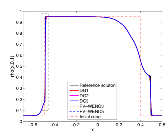
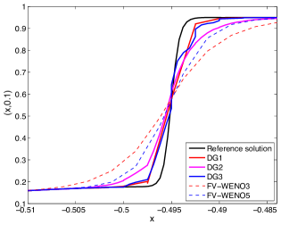
Figure 1. Test 1a. (a) Solution of Riemann problem with $w_{\eta}(x)=3(\eta^{2}-x^{2})/(2\eta^{3})$ at $T=0.1$. We compare solutions computed with FV-WENO and RKDG schemes using $\Delta x=1/800$. (b) Zoomed view of the left discontinuity in Fig (a). Reference solution is computed with FV-WENO5 with $\Delta x=1/3200$.

5.2. Test 1b: non-local LWR model

Now, we consider an initial condition with a small perturbation $\rho_{0}(x)=0.35-(x-0.5)\exp{(-2000(x-0.5)^{2})}$ and an increasing kernel function $\omega_{\eta}=2x/\eta^{2}$, with $\eta=0.05$ and periodic boundary conditions. According to [9, 17], the non-local LWR model is not stable with increasing kernels, in the sense that oscillations develop in short time. Fig. 2 displays the numerical solution with different RKDG and FV-WENO schemes with $\Delta x=1/400$ at time $T=0.3$. The profile provided by the first order scheme proposed in [9] is also included. The reference solution is computed with a FV-WENO5 scheme with $\Delta x=1/3200$. We observe that the numerical solutions obtained with the high-order schemes provide better approximations of the oscillatory shape of the solution than the first-order scheme, and that RKDG schemes give better approximations than the FV-WENO schemes.

(a)	(b)

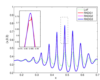
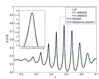
Figure 2. Test1b. Numerical solution non-local LWR model with $\omega_{\eta}=2x/\eta^{2}$, $\eta=0.05$ and $\rho_{0}(x)=0.35-(x-0.5)\exp{(-2000(x-0.5)^{2})}$. We compare solutions computed with FV Lax-Friedrichs, FV-WENO and RKDG schemes, using $\Delta x=1/400$. Reference solution is computed with FV-WENO5 with $\Delta x=1/3200$.

5.3. Test 2: non-local sedimentation model

We now solve (1.1)-(1.3)-(1.4) with the piece-wise constant initial datum

$$\rho(x,0)=\begin{cases}0&x\leq 0,\\ 0.5&0<x<1,\\ 1&x\geq 1,\end{cases}$$

with zero-flux boundary conditions in the interval $[0,1]$, and compute the solution at time $T=1$, with parameters $\alpha=1$, $n=3$ and $a=0.025$. We set $\Delta x=1/400$ and compute the solutions with different RKDG and FV-WENO schemes, including the first-order Lax-Friedrichs scheme used in [8]. The results displayed in Fig. 3 are compared to a reference solution computed with FV-WENO5 and $\Delta x=1/3200$. Compared to the reference solution, we observe that RKDG1 is more accurate than FV-WENO3, and FV-WENO5 more accurate than RKDG3 and RKDG2 (Fig. 3). In particular, we observe that the numerical solutions obtained with the high-order schemes provide better approximations of the oscillatory shape of the solution than the first order scheme. These oscillations can possibly be explained as layering phenomenon in sedimentation [29], which denotes a traveling staircases pattern, looking as several distinct bands of different concentrations. We observe in Fig. 4, where the evolution of $\rho^{h}(\cdot,t)$ is displayed for $t\in[0,5]$, that this layering phenomenon is observed with high order schemes, in this case RKDG1 and FV-WENO5, instead of Lax-Friedrichs scheme.

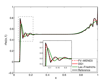
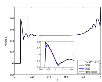
Figure 3. Test2. Riemann problem for non-local sedimentation model. Comparing numerical solution computed with FV Lax-Friedrichs, FV-WENO schemes and RKDG schemes using limiter function with $M_{b}=50$ using $\Delta x=1/400$. Reference solution is computed with FV-WENO5 with $\Delta x=1/3200$.

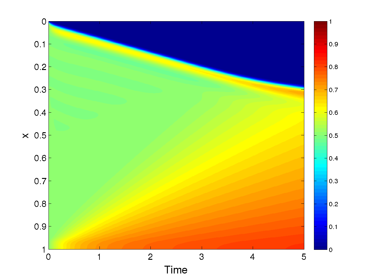
Figure 4. Test 2. Nonlocal sedimentation model. History solution for $t\in[0,5]$ computed with LxF (left) RKDG1 (center) and WENO 5 (right) with $\Delta x=1/400$. We observe that the same kind of layering phenomenon reported in [29] seems to be observed with high order schemes RKDG1 and FV-WENO5 instead of LxF scheme.

5.4. Test 3: Experimental Order of Accuracy for local conservation laws

In this subsection we compute the EOA for local conservation laws. More precisely, we first consider the advection equation $\rho_{t}+\rho_{x}=0,$ and the initial datum $\rho_{0}(x)=0.5+0.4\sin(\pi x)$ for $x\in[-1,1]$ with periodic boundary conditions. We compare the numerical approximations obtained with $\Delta x=1/M$ and $M=20,40,80,160,320,640$ at time $T=1$. RKDG schemes are used without limiting function and $L^{1}$-errors are collected in Table 1. We observe that the correct EOA is obtained for the different schemes, moreover, we observe that the $L^{1}$-errors obtained with FV-WENO3 and RKDG1 are comparable, and also the $L^{1}$-errors for FV-WENO5 and RKDG3. We also consider the nonlinear local LWR model $\rho_{t}+(\rho(1-\rho))_{x}=0,$ with initial datum $\rho_{0}(x)=0.5+0.4\sin(\pi x)$ for $x\in[-1,1]$ and periodic boundary conditions. A shock wave appears at time $T=0.3$. We compare the numerical approximations obtained with $\Delta x=1/M$ and $M=20,40,80,160,320,640$ at time $T=0.15$. RKDG schemes are used without limiters and $L^{1}$-errors are given in Table 2. We again observe that the correct EOA is obtained for the different schemes, and the $L^{1}$-errors obtained with FV-WENO3 and RKDG1 are comparable, and also the $L^{1}$-errors for FV-WENO5 and RKDG3.

	$k=1$		$k=2$		$k=3$		FV-WENO$3$		FV-WENO$5$
$\tiny{1/\Delta x}$	$L^{1}$-err	$\gamma(\Delta x)$	$L^{1}$-err	$\gamma(\Delta x)$	$L^{1}$-err	$\gamma(\Delta x)$	$L^{1}$-err	$\gamma(\Delta x)$	$L^{1}$-err	$\gamma(\Delta x)$
$20$	1.80E-03	–	9.70E-05	–	1.00E-06	–	3.72E-02	–	4.63E-04	–
$40$	4.30E-04	2.06	1.28E-05	2.92	6.04E-08	4.05	1.17E-02	1.66	1.41E-05	5.03
$80$	1.06E-04	2.02	1.63E-06	2.96	3.92E-09	3.94	2.85E-03	2.04	4.33E-07	5.02
$160$	2.64E-05	2.00	2.06E-07	2.98	2.58E-10	3.92	4.24E-04	2.74	1.35E-08	5.00
$320$	6.61E-06	2.00	2.59E-08	2.99	1.51E-11	3.32	3.06E-05	3.79	1.15E-11	5.20

Table 1. Test 3: Advection equation. Experimental order of accuracy for FV-WENO schemes and RKDG schemes without Limiter at $T=1$ with initial condition $\rho_{0}(x)=0.5+0.4\sin(\pi x)$ on $x\in[-1,1]$.

	$k=1$		$k=2$		$k=3$		WENO$3$		WENO$5$
$\tiny{1/\Delta x}$	$L^{1}$-err	$\gamma(\Delta x)$	$L^{1}$-err	$\gamma(\Delta x)$	$L^{1}$-err	$\gamma(\Delta x)$	$L^{1}$-err	$\gamma(\Delta x)$	$L^{1}$-err	$\gamma(\Delta x)$
$20$	2.03E-03	–	1.88E-04	–	5.03E-06	–	6.92E-03	–	2.80E-04	–
$40$	4.98E-04	2.02	3.06E-05	2.62	2.81E-07	4.16	2.37E-03	1.77	1.41E-05	4.31
$80$	1.23E-04	2.01	4.71E-06	2.69	1.72E-08	4.03	5.95E-04	1.99	6.14E-07	4.52
$160$	3.08E-05	2.00	7.11E-07	2.72	1.05E-09	4.02	8.20E-05	2.86	2.62E-08	4.55
$320$	7.71E-06	2.00	1.06E-07	2.74	6.62E-11	3.99	5.47E-06	3.90	8.61E-10	4.92

Table 2. Test 3: Classical LWR equation. Experimental order of accuracy for FV-WENO schemes and RKDG schemes without Limiter at $T=0.15$ with initial condition $\rho_{0}(x)=0.5+0.4\sin(\pi x)$ on $x\in[-1,1]$.

5.5. Test 4: Experimental Order of Accuracy for the non-local problems

We now consider the non-local LWR and sedimentation models. Considering the non-local LWR model, we compute the solution of (1.1)-(1.2) with initial data $\rho_{0}(x)=0.5+0.4\sin(\pi x)$ for $x\in[-1,1]$, periodic boundary conditions, with $\eta=0.1$ and $\Delta x=1/M$ and $M=80,160,320,640,1280$ at final time $T=0.15$. The results are given for different kernel functions $w_{\eta}(x)$ in Table 3. For RKDG schemes, we obtain the correct EOA. For the FV-WENO schemes, the EOA is also correct thanks to the in-cell quadratic reconstructions used to compute the non-local terms.
For the non-local sedimentation model, we compute the solution of (1.1)-(1.3)-(1.4) with initial data $\rho_{0}(x)=0.8\sin(\pi x)^{10}$ for $x\in[0,1]$ with $\eta=0.025$, $\alpha=1$, $V(\rho)=(1-\rho)^{3}$ and $\Delta x=1/M$ with $M=100,200,400,800,1600,3200$ at final time $T=0.04$. The results are given in Table 3.

		$w_{\eta}(x)=1/\eta$		$w_{\eta}(x)=2(\eta-x)/\eta^{2}$		$w_{\eta}(x)=3(\eta^{2}-x^{2})/(2\eta^{3})$
	$1/\Delta x$	$L^{1}-$error	$\gamma(\Delta x)$	$L^{1}-$error	$\gamma(\Delta x)$	$L^{1}-$error	$\gamma(\Delta x)$
FVWENO3	$40$	1.49E-03	–	1.64 -03	–	1.78E-03	–
	$80$	3.27E-04	2.18	3.39E-04	2.27	3.53E-04	2.33
	$160$	4.64E-05	2.81	4.63E-05	2.87	4.69E-05	2.91
	$320$	3.37E-06	3.78	3.44E-06	3.74	3.57E-06	3.71
	$640$	2.29E-07	3.87	2.41E-07	3.83	2.50E-07	3.83
FVWENO5	$40$	7.54E-06	–	8.65E-06	–	9.69E-06
	$80$	3.36E-07	4.48	3.75E-07	4.52	4.17E-07	4.53
	$160$	1.21E-08	4.79	1.44E-08	4.70	1.64E-08	4.66
	$320$	2.80E-10	5.43	4.52E-10	4.99	5.85E-10	4.81
	$640$	6.71E-12	5.38	1.85E-11	4.61	2.70E-11	4.43
RKDG $k=1$	$40$	4.72E-04	–	4.75E-04	–	4.76E-04	–
	$80$	1.17E-04	2.00	1.18E-04	1.99	1.19E-04	1.99
	$160$	2.94E-05	2.00	2.97E-05	1.99	2.99E-05	1.99
	$320$	7.36E-06	1.99	7.45E-06	1.99	7.49E-06	1.99
	$640$	1.84E-06	1.99	1.86E-06	1.99	1.87E-06	1.99
RKDG $k=2$	$40$	1.81E-05	–	1.21E-05	–	1.15E-05	–
	$80$	2.63E-06	2.78	1.77E-06	2.77	1.65E-06	2.80
	$160$	3.70E-07	2.82	2.54E-07	2.79	2.40E-07	2.78
	$320$	3.96E-08	2.89	3.58E-08	2.82	3.43E-08	2.80
	$640$	5.20E-09	2.93	4.03E-09	2.86	4.81E-09	2.83
RKDG $k=3$	$40$	1.93E-07	–	1.86E-07	–	1.68E-07	–
	$80$	1.21E-08	3.99	1.20E-08	3.95	1.05E-08	4.00
	$160$	7.55E-10	4.00	7.65E-10	3.97	6.65E-10	3.98
	$320$	4.87E-11	3.95	4.97E-11	3.94	4.35E-11	3.93
	$640$	3.41E-12	3.83	3.51E-12	3.82	3.15E-12	3.78

Table 3. Test 4: Non-local LWR model. Experimental order of accuracy. Initial condition $\rho_{0}(x)=0.5+0.4\sin(\pi x)$, $\eta=0.1$, numerical solution at $T=0.15$ for FV-WENO and RKDG schemes without generalized slope limiter.

	$k=1$		$k=2$		$k=3$		WENO$3$		WENO$5$
$\tiny{1/\Delta x}$	$L^{1}$-err	$\gamma(\Delta x)$	$L^{1}$-err	$\gamma(\Delta x)$	$L^{1}$-err	$\gamma(\Delta x)$	$L^{1}$-err	$\gamma(\Delta x)$	$L^{1}$-err	$\gamma(\Delta x)$
$100$	7.98E-05	–	2.90E-06	–	4.25E-07	–	2.72E-04	–	2.65E-06	–
$200$	1.98E-05	2.0	4.64E-07	2.6	3.95E-08	3.5	6.02E-05	2.1	1.01E-07	4.7
$400$	4.95E-06	2.0	7.75E-08	2.6	3.37E-09	3.6	7.87E-06	2.9	3.22E-09	4.9
$800$	1.23E-06	2.0	1.23E-08	2.6	2.47E-10	3.8	5.50E-07	3.8	1.11E-10	4.8
$1600$	3.09E-07	2.0	2.02E-09	2.6	1.22E-11	4.2	4.64E-08	3.7	4.02E-12	4.7

Table 4. Test 4: Non-local sedimentation problem. Initial condition $\rho_{0}(x)=0.8\sin(\pi x)^{10}$. Experimental order of accuracy at $T=0.04$ with $f(\rho)=\rho(1-\rho)$, $V(\rho)=(1-\rho)^{3}$, $\omega_{\eta}(x):=\eta^{-1}K(\eta^{-1}x)$ with $\eta=0.025$.

Conclusion

In this paper we developed high order numerical approximations of the solutions of non-local conservation laws in one space dimension motivated by application to traffic flow and sedimentation models. We propose to design Discontinuous Galerkin (DG) schemes which can be applied in a natural way and Finite Volume WENO (FV- WENO) schemes where we have used quadratic polynomial reconstruction in each cell to evaluate the convolution term in order to obtain the high-order accuracy. The numerical solutions obtained with high-order schemes provide better approximations of the oscillatory shape of the solutions than the first order schemes. We also remark that DG schemes are more accurate but expensive, while FV-WENO are less accurate but also less expensive. The present work thus establishes the preliminary basis for a deeper study and optimum programming of the methods, so that efficiently plots could then be considered.

References

- [1] M. Abramowitz, I. A. Stegun, et al. Handbook of mathematical functions. Applied mathematics series, 55:62, 1966.
- [2] A. Aggarwal, R. M. Colombo, and P. Goatin. Nonlocal systems of conservation laws in several space dimensions. SIAM J. Numer. Anal., 53(2):963–983, 2015.
- [3] D. Amadori, S.-Y. Ha, and J. Park. On the global well-posedness of {BV} weak solutions to the kuramoto-sakaguchi equation. Journal of Differential Equations, 262(2):978 – 1022, 2017.
- [4] D. Amadori and W. Shen. An integro-differential conservation law arising in a model of granular flow. J. Hyperbolic Differ. Equ., 9(1):105–131, 2012.
- [5] L. Ambrosio and W. Gangbo. Hamiltonian ODEs in the Wasserstein space of probability measures. Comm. Pure Appl. Math., 61(1):18–53, 2008.
- [6] P. Amorim. On a nonlocal hyperbolic conservation law arising from a gradient constraint problem. Bull. Braz. Math. Soc. (N.S.), 43(4):599–614, 2012.
- [7] P. Amorim, R. Colombo, and A. Teixeira. On the numerical integration of scalar nonlocal conservation laws. ESAIM M2AN, 49(1):19–37, 2015.
- [8] F. Betancourt, R. Bürger, K. H. Karlsen, and E. M. Tory. On nonlocal conservation laws modelling sedimentation. Nonlinearity, 24(3):855–885, 2011.
- [9] S. Blandin and P. Goatin. Well-posedness of a conservation law with non-local flux arising in traffic flow modeling. Numer. Math., 132(2):217–241, 2016.
- [10] J. A. Carrillo, S. Martin, and M.-T. Wolfram. An improved version of the Hughes model for pedestrian flow. Math. Models Methods Appl. Sci., 26(4):671–697, 2016.
- [11] B. Cockburn and C.-W. Shu. Runge-Kutta discontinuous Galerkin methods for convection-dominated problems. J. Sci. Comput., 16(3):173–261, 2001.
- [12] R. M. Colombo, M. Garavello, and M. Lécureux-Mercier. A class of nonlocal models for pedestrian traffic. Mathematical Models and Methods in Applied Sciences, 22(04):1150023, 2012.
- [13] R. M. Colombo, M. Herty, and M. Mercier. Control of the continuity equation with a non local flow. ESAIM Control Optim. Calc. Var., 17(2):353–379, 2011.
- [14] R. M. Colombo and M. Lécureux-Mercier. Nonlocal crowd dynamics models for several populations. Acta Math. Sci. Ser. B Engl. Ed., 32(1):177–196, 2012.
- [15] R. M. Colombo and F. Marcellini. Nonlocal systems of balance laws in several space dimensions with applications to laser technology. J. Differential Equations, 259(11):6749–6773, 2015.
- [16] G. Crippa and M. Lécureux-Mercier. Existence and uniqueness of measure solutions for a system of continuity equations with non-local flow. Nonlinear Differential Equations and Applications NoDEA, pages 1–15, 2012.
- [17] P. Goatin and S. Scialanga. Well-posedness and finite volume approximations of the LWR traffic flow model with non-local velocity. Netw. Heterog. Media, 11(1):107–121, 2016.
- [18] S. Göttlich, S. Hoher, P. Schindler, V. Schleper, and A. Verl. Modeling, simulation and validation of material flow on conveyor belts. Applied Mathematical Modelling, 38(13):3295 – 3313, 2014.
- [19] S. Göttlich and P. Schindler. Discontinuous Galerkin Method for Material Flow Problems. Math. Probl. Eng., pages Art. ID 341893, 15, 2015.
- [20] S. Gottlieb, D. I. Ketcheson, and C.-W. Shu. High order strong stability preserving time discretizations. Journal of Scientific Computing, 38(3):251–289, 2009.
- [21] M. Gugat, A. Keimer, G. Leugering, and Z. Wang. Analysis of a system of nonlocal conservation laws for multi-commodity flow on networks. Netw. Heterog. Media, 10(4):749–785, 2015.
- [22] A. Kurganov and A. Polizzi. Non-oscillatory central schemes for a traffic flow model with Arrehenius look-ahead dynamics. Netw. Heterog. Media, 4(3):431–451, 2009.
- [23] B. Perthame. Transport equations in biology. Frontiers in Mathematics. Birkhäuser Verlag, Basel, 2007.
- [24] B. Piccoli and F. Rossi. Transport equation with nonlocal velocity in Wasserstein spaces: convergence of numerical schemes. Acta Appl. Math., 124:73–105, 2013.
- [25] B. Piccoli and A. Tosin. Time-evolving measures and macroscopic modeling of pedestrian flow. Arch. Ration. Mech. Anal., 199(3):707–738, 2011.
- [26] J. Qiu and C.-W. Shu. Runge-Kutta discontinuous Galerkin method using WENO limiters. SIAM J. Sci. Comput., 26(3):907–929, 2005.
- [27] C.-W. Shu. Essentially non-oscillatory and weighted essentially non-oscillatory schemes for hyperbolic conservation laws. In Advanced numerical approximation of nonlinear hyperbolic equations (Cetraro, 1997), volume 1697 of Lecture Notes in Math., pages 325–432. Springer, Berlin, 1998.
- [28] C.-W. Shu and S. Osher. Efficient implementation of essentially non-oscillatory shock-capturing schemes. Journal of Computational Physics, 77(2):439–471, 1988.
- [29] D. B. Siano. Layered sedimentation in suspensions of monodisperse spherical colloidal particles. Journal of Colloid and Interface Science, 68(1):111–127, 1979.