Abstract

The complexity of matrix multiplication (hereafter MM) has been intensively studied since 1969, when Strassen surprisingly decreased the exponent 3 in the cubic cost of the straightforward classical MM to $\log_{2}(7)\approx 2.8074$. Applications to some fundamental problems of Linear Algebra and Computer Science have been immediately recognized, but the researchers in Computer Algebra keep discovering more and more applications even today, with no sign of slowdown. We survey the unfinished history of decreasing the exponent towards its information lower bound 2, recall some important techniques discovered in this process and linked to other fields of computing, reveal sample surprising applications to fast computation of the inner products of two vectors and summation of integers, and discuss the curse of recursion, which separates the progress in fast MM into its most acclaimed and purely theoretical part and into valuable acceleration of MM of feasible sizes. Then, in the second part of our paper, we cover fast MM in realistic symbolic computations and discuss applications and implementation of fast exact matrix multiplication. We first review how most of exact linear algebra can be reduced to matrix multiplication over small finite fields. Then we highlight the differences in the design of approximate and exact implementations of fast MM, taking into account nowadays processor and memory hierarchies. In the concluding section we comment on current perspectives of the study of fast MM.

2000 Math. Subject Classification:

68Q25, 65F05, 15A06, 15A69, 01A60, 15-03

Key Words:

Matrix multiplication (MM), Computations, Complexity, Linear algebra, Tensor decomposition, Multilinear algebra, Inner product, Summation, Binary Segmentation, Exact linear algebra, Small finite fields, Processors, Memory hierarchy, Impacts of fast MM, Numerical implementation, Perspectives

1 Introduction

1.1 Our subjects

Matrix multiplication (hereafter we keep using the acronym MM) is fundamentally important for symbolic and numerical computations in linear algebra and for the theory of computing. Efficient performance of MM depends on various factors, particularly on vectorization, data locality, and arithmetic cost (cf. [71, Chapter 1]).

In the first part of the paper (Sections 2–10) we review the work on the decrease of the arithmetic cost, including purely theoretical study of MM of immense sizes (so far this part of the study has been most acclaimed and most generously supported!), but we focus on feasible MM.

In our longest Section 11 we discuss realistic acceleration of symbolic MM, taking into account nowadays processor and memory hierarchies.

In our concluding Section 12 we comment on current perspectives of the study of fast MM.

1.2 History of fast MM and its impacts

The cubic arithmetic time $2n^{3}-n^{2}$ of the straightforward algorithm for $MM(n)$, that is, for $n\times n$ MM, was commonly believed to be optimal until 1969, when Strassen’s algorithm of [142] performed $MM(n)$ in $O(n^{\omega})$ time for $\omega=\log_{2}(7)\approx 2.8074$. This implied the exponent $\log_{2}(7)$ also for numerous venerated computational problems in Computer Science, Linear Algebra, and Computer Algebra such as Boolean MM, parsing context-free grammars, computing paths and distances in graphs, the solution of a nonsingular linear system of equations, computation of the inverse and the determinant of a matrix, and its various factorizations (see more in Section 10). The worldwide interest to MM has immediately exploded, and it was widely expected that new efficient algorithms would soon perform MM and solve the related computational problems in nearly quadratic time. Even the exponent 2.8074, however, defied the attacks of literally all experts around the globe for almost a decade, until 1978, when the algorithm of [113] broke Strassen’s record, improving the algorithm of [142] already at the level of feasible MM.

The mainstream research responded to that breakthrough by directing all effort to the decrease of the exponent of MM of unrestricted sizes and very soon succeeded in dramatic acceleration of infeasible MM of astronomical sizes. New surprising resources have been found, sophisticated techniques have been developed, and by 1987 the exponent of infeasible MM was decreased below 2.38 (see [44]), although as of December 2016 it still has not been decreased below 2.37, that is, in the last 3 decades the progress was nominal (see [97] for the current record exponent). Moreover, the study of infeasible MM has never made impact on practice of MM or any other realistic computations (cf. [4], [5], [21], and our concluding section).

For $n$ restricted to be “moderate”, say, less than 1,000,000, the current record is 2.7734, achieved with the algorithm of [118] and unbeaten since 1982. All algorithms supporting smaller exponents suffer from the curse of recursion (cf. [123]): they beat the classical straightforward MM algorithm only after performing a large and typically immense number of recursive steps, with the input size growing exponentially in the number of such steps: the straightforward algorithm supersedes them until the input size by far exceeds realistic level, typically by many orders of magnitude.

1.3 Focus of our presentation

In the context of this development, we refocus our presentation compared to the decades-old survey [119]. In Section 9 we still pay tribute to the lasting interest to the exponent of infeasible MM, but we do not cover various amazing sophisticated techniques proposed exclusively for the acceleration of MM of immense sizes, which dominated the review of [119]. Instead we cover in some detail the techniques that are efficient already for MM of moderate sizes and have impacts on realistic computations beyond MM. We feel that reduction of various computational problems to MM is interesting on its own right and because of potential benefits of wider application of fast or even straightforward algorithms for feasible MM. Lately the study of these links was particularly intensive in the field of symbolic computation (see, e.g., Proceedings of ISSAC 2015 and ISSAC 2016).

We recall that historically no adequate comprehensive review of the MM subject has appeared for decades, not to the benefit of the field. As we already explained, after the breakthrough of 1978, public interest to fast feasible MM was diverted by worldwide excitement about the exponent of infeasible MM, but also by some other factors. In particular the advanced techniques of of [113] were much harder for non-experts to grasp than the catchy divide and conquer method, and public attention to the fast algorithm of [113] for feasible MM was also hurt by the folk “theorem” about its alleged numerical instability. This “theorem” has somehow spread fast throughout the communities of numerical and symbolic linear algebra, before the classical paper [16] of 1980 proved that the “theorem” was false. The results of [16] became widely known only when the well-recognized article [50] extended them to all recursive bilinear algorithms for MM, but even in 2010 the Introduction of the important innovative paper [22] still referred to this “theorem”and in 2016, the paper [80] still talks about “numerical stability issues with many levels of recursions”.

Moreover the paper [50] and its successor [10] attack [113] as well as all the work on fast feasible MM from another side. Trying to simplify the discussion or perhaps to divert public attention from the advanced work on fast feasible MM to the domain of their own study and progress, the authors of these papers call “Strassen-like” all known fast algorithms for MM. This “innovation” was based on ignorance: “Strassen-like” algorithms, as [50] and [10] formally define them, have been long and well known under the much more informative name of noncommutative bilinear algorithms (see, e.g., [24]). Our personal communication in 2015 with the authors of [50] seems to help: the label “Strassen-like” is not used, e.g., in [8], but unfortunately their original widely publicized contempt to the advanced results on fast feasible MM (including those completely distinct from Strassen’s old algorithm of 1969 and in various important respects superseding it) has been deeply implanted into scientific community.

In the first part of our paper (Sections 2–10) we review the previous study of fast MM with the focus on fast feasible MM and its impacts and applications to realistic computations beyond MM, and for example we included our novel extension of an old MM technique to the computation of the inner product of 2 vectors and the summation of integers (see our Examples 8.1 and 8.2).

In the second part of the paper (Section 11) we discuss in some detail symbolic implementation of fast MM directed to minimizing communication cost and improving parallel implementation. The basic algorithms for that study are mostly decades-old, and complementing them with some more recent advanced algorithms for feasible MM is one of the most natural directions to further progress in the field.

1.4 Organization of our paper

We organize our paper as follows. In Sections 2 and 4 we recall the 2 first accelerations of MM, in 1969 and 1978, respectively, and comment on their impacts beyond MM. In Sections 3, 5, and 7 we cover the fundamental classes of bilinear, trilinear and the so called APA algorithms, respectively, and discuss the associated fundamental techniques of the algorithm design, their impact on the acceleration of MM and their links to other areas of computing and algebra. In Section 8 we extend the APA technique to computing the inner product of 2 vectors and summation. In Section 9 we summarize the history of fast MM after 1978. In Section 10 we further comment on applications of fast MM and the impact of its study to other areas of computing and Mathematics. In Section 11 we discuss applications and implementations of exact fast MM. In Section 12 we comment on numerical implementation of fast MM and perspectives of its study.

In addition to the acronym $``MM"$ for “matrix multiplication”, hereafter we write $``MI"$ for “nonsingular matrix inversion”, $MM(m,n,p)$ for $m\times n$ by $n\times p$ MM, $MM(n)$ for $M(n,n,n)$, and $MI(n)$ for $n\times n$ $MI$.

$W=(w_{i,j})_{i,j=1}^{m,n}$ denotes an $m\times n$ matrix with the entries $w_{i,j}$, for $i=1,\dots,m$ and $j=1,\dots,n$.

2 1969: from the Exponent 3 to 2.8074 by means of $2{\times}2$-based recursive processes

We begin with recalling 3 old accelerations of the straightforward MM algorithm.

Example 2.1.

From faster inner product to faster MM. [See [152] and notice technical similarity to the algorithms for polynomial evaluation with preprocessing in [111] and [92].] Observe that

$${\bf u}^{T}{\bf v}=\sum_{i=1}^{n/2}(u_{2i-1}+v_{2i})(v_{2i-1}+u_{2i})-\sum_{i=1}^{n/2}u_{2i-1}u_{2i}-\sum_{i=1}^{n/2}v_{2i-1}v_{2i},$$ (2.1)

for any even $n$. Apply this identity to all $n^{2}$ inner products defining $n\times n$ MM and compute it by using $0.5n^{3}+n^{2}$ scalar multiplications and $1.5n^{3}+2n^{2}-2n$ additions and subtractions.

Example 2.2.

Winograd’s $2\times 2$ MM (cf.  [68], [24, pages 45–46], [1, Exercise 6.5], or [52]).

Compute the product $X=UV$ of a pair of $2\times 2$ matrices,

$$U=\begin{pmatrix}u_{11}&u_{12}\\ u_{21}&u_{22}\end{pmatrix},~{}V=\begin{pmatrix}v_{11}&v_{12}\\ v_{21}&v_{22}\end{pmatrix},~{}X=UV=\begin{pmatrix}x_{11}&x_{12}\\ x_{21}&x_{22}\end{pmatrix}$$

by using the following expressions,

$s_{1}=u_{21}+u_{22}$, $s_{2}=s_{1}-u_{11}$, $s_{3}=u_{11}-u_{21}$, $s_{4}=u_{12}-s_{2}$,

$s_{5}=v_{12}-v_{11}$, $s_{6}=v_{22}-s_{5}$, $s_{7}=v_{22}-v_{12}$, $s_{8}=s_{6}-v_{21}$,

$p_{1}=s_{2}s_{6},~{}p_{2}=u_{11}v_{11},~{}p_{3}=u_{12}v_{21}$,
$p_{4}=s_{3}s_{7},~{}p_{5}=s_{1}s_{5},~{}p_{6}=s_{4}v_{22}$, $p_{7}=u_{22}s_{8}$,

$t_{1}=p_{1}+p_{2},~{}t_{2}=t_{1}+p_{4}$, $t_{3}=t_{1}+p_{5}$,
$x_{11}=p_{2}+p_{3},~{}x_{12}=t_{3}+p_{6},~{}x_{21}=t_{2}-p_{7},~{}x_{22}=t_{2}+p_{5}$.

This algorithm performs $2\times 2$ MM by using 7 scalar multiplications and 15 scalar additions and subtractions instead of 8 and 4, respectively, that is, 22 versus 12. Fix, however, a sufficiently large integer $h$, then recursively $h-1$ times substitute $2\times 2$ matrices for $u_{ij}$, $v_{jk}$, and $c_{ik}$, for all subscripts $i,j,k\in\{1,2\}$, and reuse the above algorithm for every $2\times 2$ MM. This computation only involves $7^{h}$ scalar multiplications and $7^{h-1}+15(4^{h})$ additions and subtractions, which is readily extended to performing $n\times n$ MM for any $n$ by using $c~{}n^{\log_{2}(7)}$ scalar arithmetic operations overall where $\log_{2}(7)\approx 2.8074$ and careful refinement and analysis yield $c<3.92$ [68].

Example 2.3.

Strassen’s $2\times 2$ MM [142].

$p_{1}=(u_{11}+u_{22})(v_{11}+v_{22}),~{}p_{2}=(u_{21}+u_{22})v_{11},~{}p_{3}=u_{11}(v_{12}-v_{22})$,
$p_{4}=(u_{21}-u_{11})(v_{11}+v_{12}),~{}p_{5}=(u_{11}+u_{12})v_{22},~{}p_{6}=u_{22}(v_{21}-v_{11})$, $p_{7}=(u_{12}-u_{22})(v_{21}+v_{22})$,
$x_{11}=p_{1}+p_{6}+p_{7}-p_{5},~{}x_{12}=p_{3}+p_{5},~{}x_{21}=p_{2}+p_{6},~{}x_{22}=p_{1}+p_{3}+p_{4}-p_{2}$.

This algorithm performs $2\times 2$ MM by using 7 scalar multiplications and 18 scalar additions and subtractions, which is a little inferior to Example 2.2, but also initiates a similar recursive process that performs $n\times n$ MM for any $n$ by using $c^{\prime}\cdot n^{\log_{2}(7)}$ scalar arithmetic operations for $c^{\prime}<4.54$. Being a little slower, this algorithm is used much less than Winograd’s, but is much more celebrated because it appeared earlier.

In MM literature Winograd’s algorithm is rarely called Winograd’s, but usually “Strassen–Winograd’s algorithm” or “Winograd’s variant of Strassen’s algorithm”, and sometimes less competently Strassen’s, Strassen-based, or Strassen-like (cf. [50], [10]). We can see nothing in Example 2.2 borrowed from Example 2.3, but the cited impact of [50] seems to be so deeply rooted in the Community of Computer Algebra, that even the authors of the advanced works [22] and [36] did not dare to call Example 2.2 “Winograd’s algorithm”, although their own innovative algorithms extended precisely this example and not Example 2.3.

The first line of Table 2.1 displays the estimated arithmetic cost of the recursive bilinear algorithms for $MM(n)$, $n=2^{k}$, that begin with $2\times 2$ MM by Strassen (of Example 2.3), Winograd (of Example 2.2), and Cenk and Hasan (of [36]). The second line shows the decreased cost bounds where recursive process begins with $k\times k$ MM performed with straightforward algorithm, and then one of the 3 above algorithms is applied recursively. The improvement from [36] is technically interesting, but its arithmetic cost bounds are still significantly inferior to those of the algorithms of [118] as well as ones of [94], whose implementation in [88] is numerically stable and is highly efficient in using memory space.

Table 2.1: Arithmetic Complexity of Some $2\times 2$-based Recursive Bilinear Algorithms.

Strassen’s (k=10)	Winograd’s (k=8)	Cenk and Hasan’s (k=8)
$7n^{2.81}-6n^{2}$	$6n^{2.81}-5n^{2}$	$5n^{2.81}+0.5n^{2.59}+2n^{2.32}-6.5n^{2}$
$3.89n^{2.81}-6n^{2}$	$3.73n^{2.81}-5n^{2}$	$3.55n^{2.81}+0.148n^{2.59}+1.02n^{2.32}-6.5n^{2}$

3 Bilinear Algorithms

3.1 The class of bilinear algorithms

The algorithms of Examples 2.2 and 2.3 belong to the important class of noncommutative bilinear algorithms, to which we refer just as bilinear. Such an algorithm for $MM(m,n,p)$ first computes some linear forms $l_{q}(U)$ and $l^{\prime}_{q}(V)$ in the entries of the input matrices $U=(u_{ij})_{i,j=1}^{m,n}$ and $V=(v_{jk})_{j,k=1}^{n,p}$ and then the entries $x_{ik}=\sum_{j}u_{ij}v_{jk}$ of the product $X=UV$ as the $mp$ bilinear forms,

$$l_{q}(U)=\sum_{i,j=1}^{m,n}\alpha_{ij}^{(q)}u_{ij},~{}l^{\prime}_{q}(V)=\sum_{j,k=1}^{n,p}\beta_{jk}^{(q)}v_{jk},~{}q=1,\dots,r,$$

$$x_{ik}=\sum_{q=1}^{r}\gamma_{ik}^{(q)}l_{q}(U)l^{\prime}_{q}(V),~{}~{}i=1,\dots,m;~{}k=1,\dots,p.$$

Here $r$ is said to be the rank of the algorithm, $u_{ij}$, $v_{jk}$, and $x_{ik}$ are variables or block matrices, and $\alpha_{ij}^{(q)}$, $\beta_{jk}^{(q)}$, and $\gamma_{ik}^{(q)}$ are constant coefficients for all $i,j,k$, and $q$. They define coefficient tensors $(\alpha_{ij}^{(q)})_{i,j,q}$, $(\beta_{jk}^{(q)})_{j,k,q}$, and $(\gamma_{ik}^{(q)})_{i,k,q}$, which can be also viewed as coefficient matrices

$$A=(\alpha_{ij}^{(q)})_{(i,j),q},~{}B=(\beta_{jk}^{(q)})_{(j,k),q},~{}{\rm and}~{}C=(\gamma_{ik}^{(q)})_{(i,k),q}.$$ (3.1)

3.2 The ranks of bilinear algorithms and the $MM$ exponents

Suppose $m=n=p$, assume that $u_{ij}$, $v_{jk}$, and $x_{ik}$ are block matrices, and then again recursively apply the same bilinear algorithm of rank $r$ to block matrices. The resulting bilinear algorithms have ranks $r^{h}=c^{\prime}n^{h\omega}$ for $MM(n^{h})$, $h=2,3,\dots$, $\omega=\omega_{n,r}=\log_{n}(r)$ and a constant $c^{\prime}$ is independent of $n$ and $h$. One can readily extend these observations to the following result.

Theorem 3.1.

Given a bilinear algorithm of rank $r$ for $MM(n)$ for a pair of positive integers $n$ and $r$, one can perform $MM(K)$ by using $cK^{\omega}$ arithmetic operations for any $K$, $\omega=\omega_{n,r}=\log_{n}(r)$, and a constant $c$ independent of $K$.

Now we define

(i) the exponent of MM(n),

$$\omega_{n}=\min_{r}\log_{n}(r)$$ (3.2)

where an integer $n>1$ is fixed and the minimum is over the ranks $r$ of all bilinear algorithms for $MM(n)$ and

(ii) the exponent of MM,

$$\omega=\min_{n}\omega_{n}$$ (3.3)

where the minimum is over all integers $n>1$.

(iii) The latter concept is mathematically attractive, but the highly rewarded work for its upper estimates has diverted public attention from feasible to infeasible MM. To straighten the unbalanced study of this subject, one should instead estimate the exponents of feasible MM,

$$\omega_{<N}=\min_{n<N}\omega_{n},$$ (3.4)

for realistic upper bounds $N$ on the dimension of MM inputs.

3.3 Bilinear versus quadratic algorithms for bilinear problems

The straightforward algorithm for $MM(m,n,p)$ is bilinear of rank $mnp$. The bilinear algorithms of Examples 2.2 and 2.3 for $MM(2)$ have rank 7, which turned out to be optimal (see [76], [77], [31]). [112, Theorem 3] as well as [122, Theorem 0.3] and [47]) provide an explicit expression for all bilinear algorithms of rank 7 for $MM(2)$, including the algorithms of Examples 2.2 and 2.3 as special cases. Among them 15 scalar additions and subtractions of Example 2.2 are optimal [127], [33].

One can define bilinear algorithms for any bilinear problem, that is, for the computation of any set of bilinear forms, e.g., the product of two complex numbers $(u_{1}+{\bf i}u_{2})(v_{1}+{\bf i}v_{2})=(u_{1}v_{1}-u_{2}v_{2})+{\bf i}(u_{1}v_{2}+u_{2}v_{1})$, ${\bf i}=\sqrt{-1}$. The straightforward bilinear algorithm has rank 4, and here is a rank-3 bilinear algorithm, $l_{1}l_{1}^{\prime}=u_{1}v_{1}$, $l_{2}l_{2}^{\prime}=u_{2}v_{2}$, $l_{3}l^{\prime}_{3}=(u_{1}+u_{2})(v_{1}+v_{2})$, $u_{1}v_{1}-u_{2}v_{2}=l_{1}l_{1}^{\prime}-l_{2}l^{\prime}_{2}$, $u_{1}v_{2}+u_{2}v_{1}=l_{3}l_{3}^{\prime}-l_{1}l_{1}^{\prime}-l_{2}l_{2}^{\prime}$. See [153], [65], [66], [112], [29], [78], [144], [128], [30], [31], on the early study of bilinear algorithms and see a concise exposition in [24]. The book [155] covers various efficient bilinear algorithms for multiplication of pairs of integers and polynomials (the latter operation is also called the convolution of the coefficient vectors), with further applications to the design of FIR-filters.

The minimal rank of all bilinear algorithms for a fixed bilinear problem such as $MM(m,n,p)$ is called the rank of the problem. It can be bounded in terms of the minimal arithmetic cost of the solution of the problem and vice versa [112, Theorem 1], [24].

The algorithm of Example 2.1 of rank $r=r(n)=0.5n^{3}+n^{2}$ for $MM(n)$, however, is not (noncommutative) bilinear; such algorithms are called quadratic or commutative bilinear. (See [154] on some lower bounds on the rank of such algorithms for MM.) We cannot extend to them recursive processes that bound the MM exponents by $\log_{n}(r)$, because MM is not commutative, e.g., the equation $u_{2i-1}u_{2i}=u_{2i}u_{2i-1}$ is invalid for matrices $u_{2i-1}$ and $u_{2i}$.

The algorithm, however, was of great importance in the history of fast MM: it was the first acceleration of the straightforward MM (it saves about 50% multiplications), but most important, it motivated the effort for the design of bilinear (rather than quadratic) algorithms of rank less than $n^{3}$ for $MM(n)$. It “remained” to devise such an algorithm at least for $n=2$, and Strassen received ample recognition for his brilliant design that accomplished exactly this.

4 1978: from 2.81 to 2.78 by means of trilinear aggregation

In 1969 the exponents below Strassen’s 2.8074 became the target of literally all the leading researchers in the field, worldwide, but remained a dream for almost a decade. This dream would have come true based on bilinear algorithms of rank 6 for $MM(2)$ or rank 21 for $MM(3)$, but it was proved that the rank of $MM(2)$ exceeds 6, and it is still unknown whether $MM(3)>22$.

We refer the reader to the paper [100] for the current record lower bounds on the rank of $MM(n)$ for all $n$, to the papers [76], [77], [112, Theorem 1], and [29], [31], [32], [20], [19], [129], [137], and [95] for some earlier work in this direction, and to the papers [53] and [136] for various lower and upper bounds on the arithmetic complexity and the ranks of rectangular MM of smaller sizes.

The exponent was decreased only in 1978, after almost a decade of stalemate, when the paper [113] presented a bilinear algorithm of rank 143,640 for $MM(70)$. This breakthrough implied the exponent $\omega=\log_{70}(143,640)<2.7962$ for $MM(n)$, $MI(n)$, Boolean $MM(n)$, and a variety of other well-known computational problems. The algorithm of [113] has extended an algorithm of the paper [112] of 1972, published in Russian and translated into English only in 2014 in [122].

The progress was due to the novel combination of two techniques: trilinear interpretation of bilinear algorithms and the aggregation method. By following [113] we call this combination trilinear aggregation. By refining this combination of 2 techniques the paper [118] accelerated MM of moderate sizes and yielded the exponent 2.7734. As we already mentioned, various algorithms combining trilinear aggregation with other advanced techniques decreased the exponent below this level (and in 1986 even below 2.38), but only when they were applied to MM of immense sizes because of the curse of recursion.

The technique of trilinear aggregation has been recognized for its impact on the decreases of the MM exponent, but the paper [112] was also a historical landmark in the study of multilinear and tensor decompositions. Such decompositions introduced by Hitchcock in 1927 received little attention except for a minor response in 1963–70 with half of a dozen papers in the psychometrics literature. The paper [112] of 1972 provided the earliest known application of nontrivial multilinear and tensor decompositions to fundamental matrix computations, now a popular flourishing area in linear and multilinear algebra with a wide range of important applications to modern computing (see [148], [93], [108], [71], and the bibliography therein). Nevertheless the paper [112] has rarely been cited at all and has never been cited in the papers on multilinear and tensor decompositions.

5 Trilinear Decompositions and Duality

Next we define trilinear representation of MM, first proposed and used in the paper [112]. We are also going to link it to some important computations beyond MM.

Let $U=(u_{ij})_{i,j}$ and $V=(v_{jk})_{j,k}$ be a pair of $m\times n$ and $n\times p$ matrices, respectively, and let the equations $\sum_{j}u_{ij}v_{jk}=\sum_{s=1}^{r}w_{ik}^{(s)}l_{s}(U)l^{\prime}_{s}(B)$ for all $i,j$ represent a bilinear algorithm of rank $r$ for the matrix product $X=UV$.

Define a trilinear decomposition of rank $r$ for $trace(UVW)=\sum_{i,j,k}u_{i,j}v_{jk}w_{ki}$ by multiplying these equations by variables $d_{ki}$ and summing the products in $i$ and $k$. Here $W=(w_{ki})_{k,i}^{n,m}$ is an auxiliary $n\times m$ matrix and trace$(M)$ denotes the trace of a matrix $M$. (Equivalently we can decompose the tensor of the trilinear form $trace(UVW)$ into the sum of $r$ tensors of rank 1.)

Example 5.1.

A trilinear decomposition of rank 7 for $MM(2)$.
$~{}~{}~{}~{}~{}~{}~{}~{}~{}\sum_{i,j,h=1}^{2}u_{ij}v_{jh}w_{hi}=\sum_{s=1}^{7}l_{s}l_{s}^{\prime}l_{s}^{\prime\prime}$,  $l_{1}l_{1}^{\prime}l_{1}^{\prime\prime}=(u_{11}+u_{22})(v_{11}+v_{22})(w_{11}+w_{22})$,
$l_{2}l_{2}^{\prime}l_{2}^{\prime\prime}=(u_{21}+u_{22})v_{11}(w_{21}-w_{22})$, $l_{3}l_{3}^{\prime}l_{3}^{\prime\prime}=u_{11}(v_{12}-v_{22})(w_{12}+w_{22})$, $l_{4}l_{4}^{\prime}l_{4}^{\prime\prime}=(u_{21}-u_{11})(v_{11}+v_{12})w_{22}$,
$l_{5}l_{5}^{\prime}l_{5}^{\prime\prime}=(u_{11}+u_{12})v_{22}(w_{12}-w_{11})$, $l_{6}l_{6}^{\prime}l_{6}^{\prime\prime}=u_{22}(v_{21}-v_{11})(w_{11}+w_{21})$, $l_{7}l_{7}^{\prime}l_{7}^{\prime\prime}=(u_{12}-u_{22})(v_{21}+v_{22})w_{11}$.

Conversely, we can come back to the original bilinear algorithm for the matrix product $X=UV$ if we interpret both sides of any decomposition of the trilinear form $trace(UVW)$ as linear forms in the variables $w_{ih}$ and equate the coefficients of these variables on both sides of the decomposition.

More generally, [112, Theorem 2] states the equivalence of a bilinear algorithm of rank $r$ for $MM(m,n,p)$ to a trilinear decomposition of rank $r$ for the associated trilinear form and its tensor.

Instead of equating the variables $w_{ij}$ on both sides of the trilinear decomposition, we can equate the coefficients of all variables $u_{ij}$ or all variables $v_{jh}$ and then arrive at 2 other dual bilinear algorithms of the same rank for the problems $M(n,p,m)$ and $M(p,m,n)$.

By interchanging the subscripts of the variables, we arrive at the dual bilinear algorithms of the same rank for the problems $MM(m,p,n)$, $MM(n,m,p)$, and $MM(p,n,m)$ as well (cf. [112, part 5 of Theorem 1], [29], [78], [128]). The latter extension from triples to 6-tuples is pertinent to MM, because it uses the double subscripts for the variables, but the triples of bilinear algorithms can be generated from their common trilinear representation for any bilinear computational problem, e.g., for multiplication of 2 complex numbers in the following example.

Example 5.2.

A trilinear decomposition of rank 3 for multiplication of 2 complex numbers.

$$u_{1}v_{1}w_{1}-u_{2}v_{2}w_{1}+u_{1}v_{2}w_{2}+u_{2}v_{1}w_{2}=u_{1}v_{1}(w_{1}-w_{2})-u_{2}v_{2}(w_{1}+w_{2})+(u_{1}+u_{2})(v_{1}+v_{2})w_{2}.$$

For a sample application of the duality technique, one can readily deduce the following result (part 1 of [112, Theorem 1]).

Theorem 5.1.

Given a bilinear or trilinear algorithm of rank $r$ for $MM(m,n,p)$ and any 4-tuple of integers $r$, $m$, $n$, and $p$ such that $mnp>1$, one can perform $MM(K)$ by using $cK^{\omega}$ arithmetic operations for any $K$, $\omega=\omega_{m,n,p,r}=3\log_{mkn}(r)$, and a constant $c$ independent of $K$.

For further applications of the duality technique, see efficient bilinear algorithms for FIR-filters and multiplication of complex numbers and polynomials in [155].

6 Trilinear Aggregation

Aggregation technique is well-known in business, economics, computer science, telecommunication, natural sciences, medicine, and statistics. The idea is to mass together or cluster independent but similar units into much fewer aggregates. Their study is simpler, but its results are supposed to characterize all these units either directly or by means of special disaggregation techniques. Such aggregation/disaggregation processes proposed in [101] became a basis for creating the field of Algebraic Multigrid, now quite popular.

Aggregation/disaggregation techniques are behind the acceleration of MM in Example 2.1, which was preceded by similar application of this technique to polynomial evaluation with preprocessing of coefficients [111], [92]. In that example one first rewrite $u_{2i}v_{2i}=v_{2i}u_{2i}$ by using commutativity of multiplication (which does not hold if $u_{2i}$ and $v_{2i}$ are matrices), then aggregates the terms $u_{2i-1}v_{2i-1}$ and $v_{2i}u_{2i}$ into the single term $(u_{2i-1}+v_{2i})(v_{2i-1}+u_{2i})$, thus saving 50% of scalar multiplications, that is, $0.5n^{3}$ for $n\times n$ MM. For disaggregation one subtracts the correction terms $u_{2i-1}u_{2i}$ and $v_{2i}v_{2i-1}$. $n\times n$ MM involves $0.5n^{2}$ pairs of such products, and so correction involves just $n^{2}$ scalar multiplications overall, which is a small sacrifice compared to saving $0.5n^{3}$ scalar multiplications.

The papers [112] and [113] strengthen aggregation based on restating MM as the problem of the decomposition of the trilinear form $trace(UVW)$, so that some additional links among the subscripts of the input and output entries enable stronger aggregation and faster MM.

Various implementations of this technique appeared in [113], [114], [115], and a number of subsequent papers. For demonstration we apply it to Disjoint MM where we compute two independent matrix products $AB$ and $UV$ by decomposing the trilinear form $trace(XYZ+UVW)=\sum_{i,j,k=1}^{m,n,p}(x_{ij}y_{jk}z_{ki}+u_{jk}v_{ki}w_{ij})$ into the sum of rank-1 tensors.

Let $T=\sum_{i,j,k=1}^{m,n,p}(x_{ij}+u_{jk})(y_{jk}+v_{ki})(z_{ki}+w_{ij})$ denote a trilinear aggregate made up of the 2 monomials $x_{ij}y_{jk}z_{ki}$ and $u_{jk}v_{ki}w_{ij}$ and let $T_{1}=\sum_{i,j=1}^{m,n}x_{ij}s_{ij}w_{ij}$, $T_{2}=\sum_{j,k=1}^{n,p}u_{jk}y_{jk}r_{jk}$, and $T_{3}=\sum_{k,i=1}^{p,m}q_{ik}v_{ki}z_{ki}$ denote 3 groups of correction terms, where $q_{ik}=\sum_{j=1}^{k}(u_{ij}+u_{jk})$, $s_{ij}=\sum_{k=1}^{n}(y_{jk}+v_{ki})$, and $r_{jk}=\sum_{i=1}^{m}(z_{ki}+w_{ij})$. Then the equation $trace(XYZ+UVW)=T-T_{1}-T_{2}-T_{3}$ defines a trilinear decomposition of rank $mnp+mn+np+pm$ (rather than the straightforward $2mnp$).

Table 6.1 displays this aggregation/disaggregation technique.

Table 6.1: Aggregation/disaggregation of a pair of terms.

$x_{ij}$	$y_{jk}$	$z_{ki}$
$u_{jk}$	$v_{ki}$	$w_{ij}$

The product of the 3 sums of pairs on input entries in each of the 3 columns of the table is an aggregate. The 2 products of triples of entries of each of the 2 rows are the output terms $x_{ij}y_{jk}z_{ki}$ and $u_{jk}v_{ki}w_{ij}$. The cross-products of other triples of the table define 6 correction terms. Their sum over all $n^{3}$ triples of indices $i,j$ and $k$ has rank $2(mn+np+pm)$. By subtracting this sum from the sum of all $mnp$ aggregates, we decompose $2mnp$ terms of $trace(XYZ+UVW)$ into the sum of $mnp+2(mn+np+pm)$ terms. For $m=n=p=34$ this implies a decomposition of rank $n^{3}+6n^{2}$ for a pair of disjoint $MM(n)$.

Demonstration of the power of trilinear aggregation can be made most transparent for Disjoint MM, whose natural link to trilinear aggregation has been shown in [119], [120, Section 5], [121, Section 12], and [94]. Such constructions for Disjoint MM, however, can frequently be extended to $MM(n)$. In particular, by playing with odd and even subscripts of the matrix entries, the paper [112] obtained a trilinear decomposition of rank $0.5n^{3}+3n^{2}$ for $MM(n)$ and any even $n$ by means of extending the above decomposition of $trace(XYZ+UVW)$. This implied the $MM$ exponent $\log_{n}(0.5n^{3}+3n^{2})$, which is less than 2.85 for $n=34$.

The paper [113] defined a trilinear decomposition and bilinear algorithms of rank $(n^{3}-4n)/3+6n^{2}$ for $MM(n)$, $n=2s$, and any positive integer $s$. Substitute $n=70$ and obtain the MM exponent 2.7962. Then again it is convenient to demonstrate this design for Disjoint MM associated with a decomposition of the trilinear form $trace(XYZ+UVW+ABC)$. The basic step is the aggregation/disaggregation defined by Table 6.2.

Table 6.2: Aggregation/disaggregation of a triple of terms.

$x_{ij}$	$y_{jk}$	$z_{ki}$
$u_{jk}$	$v_{ki}$	$w_{ij}$
$a_{ki}$	$b_{ij}$	$c_{jk}$

Sum the $mkn$ aggregates $(x_{ij}+u_{jk}+a_{ki})(y_{jk}+v_{ki}+b_{ij})(z_{ki}+w_{ij}+c_{jk})$, subtract order of $n^{2}$ correction terms, and obtain a decomposition of rank $n^{3}+O(n^{2})$ for $trace(XYZ+UVW+ABC)$, versus the straightforward $3n^{3}$. The trace represents 3 disjoint problems of $MM(n)$, that is, the computation of the 3 independent matrix products $XY$, $UV$, and $AB$ of size $n\times n$ (and can be readily extended to 3 MM products of sizes $m\times n$ by $n\times p$, $n\times p$ by $p\times m$, and $p\times m$ by $m\times n$), and we obtain a bilinear algorithm of rank $n^{3}+O(n^{2})$ for this bilinear task.

With a little more work one obtains a similar trilinear decomposition of rank $(n^{3}-4n)/3+6n^{2}$ for $MM(n)$, $n=2s$, and any positive integer $s$ (see [113]). For $n=70$ we arrive at an upper bound 2.7962 on the MM exponent. By refining this construction the algorithm of [118] decreased the upper bound below 2.7734.

7 APA Algorithms and Bini’s Theorem

The technique of Any Precision Approximation (hereafter we use the acronym APA) was another basic ingredient of the algorithms supporting the decrease of the exponent of MM. The paper [15] achieved the first APA acceleration of MM, by yielding the exponent 2.7799. According to [130], this came from computer search for partial $MM(2)$ where the goal was the computation of only 3 entries of $2\times 2$ matrix product.

Next we demonstrate the combination of APA and trilinear aggregation, which is more transparent and immediately produces the exponent 2.66. Consider the following table.

Table 7.1: APA aggregation/disaggregation of a pair of terms.

$x_{ij}$	$y_{jk}$	$\lambda^{2}z_{ki}$
$\lambda u_{jk}$	$\lambda v_{ki}$	$w_{ij}$

It defines the aggregate $(x_{ij}+\lambda u_{jk})(y_{jk}+\lambda v_{ki})(\lambda^{2}z_{ki}+w_{ij})$ and 3 correction terms, similarly to Table 6.1, but with a decisive difference – the term $\lambda^{3}(x_{ij}+u_{jk})v_{ki}z_{ki}$ has a smaller order of magnitude as $\lambda\rightarrow 0$. Therefore we arrive at trilinear decomposition

$$trace(XYZ+UVW)=T-T_{1}-T_{2}+O(\lambda)$$

where

$$T=\lambda^{-1}\sum_{i,j,k=1}^{m,k,n}(x_{ij}+\lambda u_{jk})(y_{jk}+\lambda v_{ki})(\lambda^{2}z_{ki}+w_{ij}),~{}T_{1}=\sum_{i,j=1}^{m,k}x_{ij}s_{ij}w_{ij},~{}T_{2}=\sum_{j,k=1}^{k,n}u_{jk}y_{jk}r_{jk},$$

$s_{ij}=\sum_{k=1}^{n}(y_{jk}+\lambda v_{ki})$, and $r_{jk}=\sum_{i=1}^{m}(\lambda^{2}z_{ki}+w_{ij})$.

Drop the terms of order $\lambda$, and obtain a decomposition for Disjoint $MM(m,n,p)$ having border rank $mnp+mn+np$. For $m=p=7$, $n=1$ this implies an APA exponent of MM $\omega=3\log_{49}31.5<2.66$. (Here we use Schönhage’s result of [133] that deduces the MM exponent from Disjoint MM.)

The above APA decomposition using $mnp+mn+np$ terms is numerically unstable. Indeed we would corrupt the output if we drop the summands $\lambda u_{jk}$ and $\lambda v_{ki}$ in the sums $x_{ij}+\lambda u_{jk}$ and $y_{jk}+\lambda v_{ki}$ in the aggregate $(x_{ij}+\lambda u_{jk})(y_{jk}+\lambda v_{ki})(\lambda^{2}z_{ki}+w_{ij})$, but keeping these summands doubles the precision required for the representation of these sums. Similarly all other known bilinear APA algorithms are prone to numerical stability problems if their rank exceeds their border rank.

In [14], however, Bini proved that, for the purpose of decreasing the exponent of MM, this deficiency is immaterial if we allow unrestricted recursive processes, that is, if we ignore the curse of recursion. Namely he proved that Theorem 5.1 holds even if border rank replaces rank in its statement. Bini proved this result for MM, but Schönhage in [133] extended it to Disjoint MM. Both proofs yield acceleration of straightforward MM only where its input size becomes huge because of the curse of recursion.

Theorem 7.1.

We can perform $MM(K)$ by using $\bar{c}K^{\omega}$ arithmetic operations for any $K$, where $\bar{c}$ is a constant independent of $K$ and $\omega=\omega_{m,n,p,r}=3\log_{mkn}(r)$, provided that we are given a bilinear or trilinear APA algorithm having a border rank $r$ for $MM(m,n,p)$ and a 4-tuple of integers $r$, $m$, $n$, and $p$ such that $mnp>1$.

Proof.

First observe that by means of interpolation we can extend any APA algorithm of border rank $r$ using a polynomial $q(\lambda)$ in $\lambda$, of a degree $d$ to a $\lambda$-free bilinear algorithm for $MM(m,n,p)$ of rank $(2d+1)r$.

Now apply such an APA algorithm recursively. Notice that every recursive step squares the original problem size $mnp$ but only doubles the degree of $\lambda$. After $h$ steps, we arrive at an APA algorithm of degree $2^{h}d$ for the MM problem of size $(mnp)^{2^{h}}$, and then (cf. Theorem 5.1) the interpolation factor $2(2^{h}d+1)$ only implies an increase of the MM exponent $\omega$ by a tiny factor, which converges to 1 as the number of recursive steps grows to the infinity. ∎

8 Inner Product Computation and Summation by Means of APA Techniques

Next we cover an application of APA techniques beyond MM.

Recall the APA algorithm of Section 7, let the entries $x_{ij}$, $y_{jk}$, $u_{jk}$, and $v_{ki}$ be integers in the range $[0,2^{d})$, and choose $\lambda=2^{d}$. Notice that the product $(x_{ij}+\lambda y_{jk})(u_{jk}+\lambda v_{ki})$ fits the length $L$ of the computer word if $L\geq 4d$. Moreover if the ratio $L/d$ is large enough, we can perform the APA computations of Section 7 within the precision $L$. [121, Section 40] exploits such observations further and devise efficient algorithms for multiplication of vectors and matrices filled with bounded integers. Next we recall that technique and in Example 8.2 show its surprising extension.

Suppose that the coefficient vector of a polynomial $v(\lambda)=\sum_{i=0}^{n-1}v_{i}\lambda^{i}$ is filled with integers from the semi-open segment $[0,2^{d})$ of the real axis for a positive integer $d$. Represent this vector by the $2^{d}$-ary integer $v(2^{d})=\sum_{i=0}^{n-1}v_{i}2^{di}$. Generally the interpolation to a polynomial of degree $n-1$ requires its evaluation at $n$ knots, but in the above special case we only need the evaluation at the single knot $2^{d}$. Now suppose that all coefficients $v_{i}$ are integers from the semi-open segment $[q,r)$ for any pair of integers $q$ and $r$, $q<r$. Then we can apply the above recipe to compute the shifted vector ${\bf u}=(u_{i})_{i=0}^{n-1}=(v_{i}-q)_{i=0}^{n-1}$, having all its components in the semi-open segment $[0,s)$ for $s=r-q$. We can finally recover the vector ${\bf v}$ from ${\bf u}$. By following [116] and [17], we call this technique binary segmentation. Its history can be traced back to [67], and one can even view it as an application of the Kronecker map, although having specific computational flavor.

Next we follow [121, Example 40.3, pages 196–197] to compute the inner product of two integer vectors, then extend the algorithm to summation, and finally list various other applications of binary segmentation.

Example 8.1.

(The inner product of two integer vectors, cf. [121, Example 40.3].) Assume two nonnegative integers $g$ and $h$ and two vectors ${\bf u}=(u_{i})_{i=0}^{n-1}$ and ${\bf v}=(v_{i})_{i=0}^{n-1}$ with nonnegative integer coordinates in two semi-open segments, namely, $[0,2^{g})$ for the coordinates of ${\bf u}$ and $[0,2^{h})$ for the coordinates of ${\bf v}$. The straightforward algorithm for the inner product ${\bf u}^{T}{\bf v}=\sum_{i=0}^{n-1}u_{i}v_{i}$ first computes the $n$ products $u_{i}v_{i}$ for $i=0,1,\dots,n-1$ and then sums them. This involves $n$ multiplications and $n-1$ additions. Instead, however, we can just multiply a pair of bounded nonnegative integers, apply binary segmentation to the product, and output the desired inner product. Namely, introduce the two polynomials $u(x)=\sum_{i=0}^{n-1}u_{i}x^{i}$ and $v(x)=\sum_{i=0}^{n-1}v_{i}x^{n-1-i}$. Their product is the polynomial $q(x)=u(x)v(x)=\sum_{i=0}^{2n-2}q_{i}x^{i}$ with integer coefficients in the segment $[0,2^{k})$ for $k=g+h+\lceil\log_{2}n\rceil$. The coefficient $q_{n-1}=\sum_{i=0}^{n-1}u_{i}v_{i}$ is precisely the inner product ${\bf u}^{T}{\bf v}$. Represent the polynomials $u(x)$ and $v(x)$ by their integer values $u(2^{k})$ and $v(2^{k})$ at the point $2^{k}$. Clearly, they lie in the semi-open segments $r_{u}=[0,2^{nk+g})$ and $r_{v}=[0,2^{nk+h})$, respectively. Now compute the integer $q(2^{k})=u(2^{k})v(2^{k})$, lying in the segment $[0,2^{2nk+g+h})$, and recover the coefficient $q_{n-1}={\bf u}^{T}{\bf v}$ by applying binary segmentation.

Remark 8.1.

We only seek the coefficient $q_{n-1}$ of the median term $q_{n-1}x^{n-1}$ of the polynomial $u(x)v(x)$. This term lies in the segment $[2^{(n-1)k},2^{(n-1)k+g+h})$, and the next challenge is to optimize its computation. Is such a more narrow task substantially simpler than the multiplication of two integers lying in the segments $r_{u}$ and $r_{v}$?

Example 8.2.

(Summation of bounded integers.) For ${\bf u}=(1)_{i=0}^{n-1}$, $g=0$, and $k=h+\lceil\log_{2}n\rceil$ or ${\bf v}=(1)_{i=0}^{n-1}$, $h=0$, and $k=g+\lceil\log_{2}n\rceil$, the algorithm of Example 8.1 outputs the sum of $n$ integers.

Remark 8.2.

In the same way as for polynomial interpolation in the beginning of this section, we can relax the assumption of Examples 8.1 and 8.2 that the input integers are nonnegative. Moreover, the summation of integers can be extended to the fundamental problem of the summation of binary numbers truncated to a fixed precision.

In Examples 8.1 and 8.2, multiplication of two long integers followed by binary segmentation replaces either $2n-1$ or $n$ arithmetic operations, respectively. This increases the Boolean (bit-wise operation) cost by a factor depending on the Boolean cost of computing the product of 2 integers or, in view of Remark 8.1, of computing the median segment in the binary representation of the product. The increase is minor if we multiply integers in nearly linear Boolean time (see the supporting algorithms for such multiplication in [135], [1, Section 7.5], [69]), but grows if we multiply integers by applying the straightforward algorithm, which uses quadratic Boolean time. Nonetheless, in both cases one could still benefit from using Example 8.2 if the necessary bits of the output integer fit the computer word (i.e. the bits of the middle coefficient are not part of the overflow of the product), as long as the representation of the vector as an integer requires no additional cost. If the output integer does not fit the word length, we can apply the same algorithms to the subproblems of smaller sizes, e.g., we can apply the algorithms of Examples 8.1 and 8.2 to compute the inner products of some subvectors or partial sums of integers, respectively.

Other applications of binary segmentation include polynomial multiplication (that is, the computation of the convolution of vectors) [67], [134], some basic linear algebra computations [121, Examples 40.1–40.3], polynomial division [17], [134], computing polynomial GCD [37], and discrete Fourier transform [134]. Binary segmentation can be potentially efficient in computations with Boolean vectors and matrices. E.g., recall that Boolean MM is reduced to MM whose input and output entries are some bounded nonnegative integers (see [1, Proof of Theorem 6.9]). Quantized tensor decompositions is another promising application area (cf. [148], [106], [107], [91], [109], [72]).

9 Summary of the Study of the MM Exponents after 1978

In 1979–81 and then again in 1986 the exponent of infeasible MM was significantly decreased based on combination of trilinear aggregation, Disjoint MM, and APA techniques with unrestricted use of recursion.

All supporting algorithms have been built on the top of the techniques of the preceding papers.

More and more lenient basic bilinear/trilinear decompositions of small rank were chosen for Disjoint MM of small sizes and since 1986 for small bilinear/trilinear problems similar to Disjoint MM. Transition back to MM relied on nested recursion, consistently intensified; consequently acceleration of the straightforward algorithm began only with MM of astronomical sizes.

By 1987 the power of these techniques seems to be exhausted, and then the progress has stopped until 2010. Since then it is moving from the bound 2.376 of [44] towards 2.37 with the snail’s speed.

That direction was prompted by the cited results of the seminal papers [14] by Dario Bini and [133] by Arnold Schönhage. Schönhage, however, has concluded the introduction of [133] with pointing out that all new exponents of MM were just ”of theoretical interest” because they were valid only for the inputs ”beyond any practical size” and that ”Pan’s estimates of 1978 for moderate” input sizes were ”still unbeaten”. Actually, as we can see in Figure 1, the exponent 2.7962 of 1978 for $MM(n)$ restricted to $n\leq 1,000,000$ has been successively decreased in [114], [115], [117], and [118] (cf. also [119]), although by small margins. As of December 2016, the exponent 2.7734 of [118] is still record low for $MM(n)$ with $n\leq 1,000,000$.

Figures 1 and 2 display chronological decrease of the exponents of $MM(n)$ for $n\leq 1,000,000$ and for unrestricted $n$, respectively. The supporting algorithms of Figure 1 rely solely on trilinear aggregation, and the associated overhead constants are small. Some of these algorithms have been refined in [119], [94] and implemented in [87] and [88].

All other algorithms of Figure 2 (not supporting Figure 1) employ trilinear aggregation as well (cf. [44, page 255]), but also employ other techniques and suffer from the curse of recursion.

The figures link each exponent to its recorded publication in a journal, a conference proceedings, or as a research report. As we already mentioned, the MM exponent of [113] significantly decreased in 1979–1981 and 1986. It has been updated at least 4 times during the single year of 1979: reaching below the values 2.801 in February in Research Report [115]; 2.7799 (as an APA MM exponent) in [15] in June and (as an MM exponent) in [14]; 2.548 in [133], and 2.522 in [117]. Both of the latter two exponents appeared in the book of abstracts of the conference on the Computational Complexity in Oberwolfach, West Germany, organized by Schnorr, Schönhage and Strassen in October (cf. [119, page 199] and [133]). The exponent 2.496 of [43] was reported in October 1981 at the IEEE FOCS’81, and in Figure 1 we place it after the exponent 2.517 of the paper [131] of 1982, which was submitted in March 1980. The Research Report version of the paper [44] appeared in August of 1986, but in Figure 2 we place [44] after the paper [146], published in October of 1986 in the Proceedings of the IEEE FOCS, because the paper [146] has been submitted to FOCS’86 in the Spring of 1986 and has been widely circulated afterwards. One could complete the historical account of Figure 2 by including the exponents 2.7804 (announced in the Fall of 1978 in [113] and superseded in February 1979 when the paper was submitted [115]) and 2.5218007, which decreased the exponent 2.5218128 of [114] and appeared at the end of the final version of [133] in 1981, that is, before the publication, but after the submission of the exponent 2.517 of [131].

We refer the reader to [41], [99], [42], [79], [89], [96], and the references therein for similar progress in asymptotic acceleration of rectangular MM.

Figure 1: $MM(n)$ exponents for $n\leq 1,000,000$.

Figure 2: $MM(n)$ exponents for unrestricted $n$.

10 Applications of Fast MM, Its Links to Other Subject Areas, Impacts of Its Study, and Implementation (Briefly)

The decrease of the exponent of MM implies theoretical acceleration of the solution of a number of important problems in various areas of computations in Algebra and Computer Science, such as Boolean MM, computation of paths and distances in graphs, parsing context-free grammars, the solution of a nonsingular linear system of equations, computations of the inverse, determinant, characteristic and minimal polynomials, and various factorizations of a matrix.

See [142], [34], [1, Sections 6.3–6.6], [24, pages 49–51], [18, Chapter 2], [3], [79], [48], [98], [160], [157], [158], [159], [86], [25], [89], [6], [54], [156], [132], [96], [4], [138], [140], [103], [104], [105], [125], and the bibliography therein and notice that some new important applications have been found very recently, e.g., in 4 papers at ISSAC 2016.

The reduction of other computational problems to MM increases the overhead, which is already immense for the algorithms supporting the record exponent of MM. Such a reduction, however, can still be valuable because it reveals some links of independent interest and because by applying fast algorithms or even the straightforward algorithm for feasible MM one can take advantage of using block matrix software and parallel acceleration.

Research on fast feasible MM had a variety of feasible links to other subject areas. The work on bilinear and trilinear decompositions for fast MM was an important part of the study of such decompositions in the general area of Algebraic Computations and has led to new insights and techniques.

• We have already cited historical importance of the demonstration in 1972 in [112] of the power of tensor decompositions and valuable applications of duality to the design of efficient bilinear algorithms.

• Trilinear aggregation was also a surprising demonstration of the power of aggregation/disaggregation methods.

• More applications of this kind can follow in the future, such as a quite unexpected application of APA techniques to the computation of inner products and summation presented in Section 8.

• It may be surprising, but apart from trilinear aggregation and the APA method, the advanced and amazing techniques developed for decreasing the exponent of infeasible MM had no theoretical (as well as practical) applications to other areas of computations or algebra (and have made no impacts on actual work on MM as well).

Of course, such impacts on the practice of performing this fundamental operation of modern computations are the main motivation and goal of the study of fast MM, and indeed recursive bilinear algorithms based on $2\times 2$ Strassen’s and particularly Winograd’s brilliant designs of Examples 2.3 and 2.2, respectively, are a valuable part of modern software for MM.

In Section 1.3 we commented on numerical stability issues for fast feasible MM, and we refer the reader to [12], [73], [52], [61], [62], [28], [45], [71, Chapter 1], [13], [8], [11], and the bibliography therein for their previous and current numerical implementation. In the next section we discuss symbolic application of the latter algorithm (WRB-MM) in some detail.

It is very encouraging to observe dramatic increase of the activity in numerical and symbolic implementation of fast MM in recent years, towards decreasing communication cost and improving parallel implementation, in good accordance with the decrease of the arithmetic cost.

11 Fast methods in exact computational linear algebra

Next we discuss applications and implementations of exact fast matrix multiplication (MM). As we mentioned in Section 1.1, we first review how most of the exact linear algebra can be reduced to MM over small finite fields. Then we highlight the differences in the design of approximate and exact implementations of MM taking into account nowadays processor and memory hierarchies.

11.1 Acceleration of computations via reductions to MM

The design of matrix multiplication routines over a word size finite field is the main building block for computations in exact dense linear algebra, represented with coefficient domains of two kinds: word-size discrete entries (mainly in finite fields of small cardinality) and variable size entries (larger finite fields, integers, or polynomials). Indeed, efficient methods for the latter task usually reduce it to the former one: reductions are made by means of evaluation/interpolation (Chinese remaindering over the integers) or by means of lifting small size solutions (via Hensel-like or high-order lifting [139]), see, e.g., [85, 63, 124] for recent surveys.

Over word-size finite fields, efficient implementations of MM have been obtained by means of effective algorithmic reductions originated in the complexity analysis. In this case reductions have been obtained directly to MM. Already Strassen in 1969 extended MM to matrix inversion (we sketch this in Examples 11.1 and 11.2 below), then Bunch and Hopcroft [34] extended MM to invertible LUP factorization, and further extensions followed in the eighties, for instance, in [82] to the computation of the matrix rank and of Gaussian elimination. Efficient algorithms whose complexity is sensitive to the rank or to the rank profile have only very recently been discovered [83, 64, 140]. One of the latest reductions to MM was that of the characteristic polynomial, which has extended the seminal work of [90] more than thirty years afterwards [126].

Example 11.1.

Triangular system solving by means of reduction to matrix multiplication.
Denote by $X=TRSM(U,B)$ the solution to the linear matrix equation $UX=B$ with a matrix $B$ on the right-hand side and an upper triangular invertible matrix $U$. Recursively cut the matrices $U$, $B$ and $X$ in halves as follows: $U=\begin{bmatrix}U_{1}&V\\ &U_{2}\end{bmatrix}$, $X=\begin{bmatrix}X_{1}\\ X_{2}\end{bmatrix}$, and $B=\begin{bmatrix}B_{1}\\ B_{2}\end{bmatrix}$; then obtain an efficient reduction of the solution to MM by means of the following algorithm:

1. Recursively compute $X_{2}=TRSM(U_{2},B_{2})$;

2. Compute $B^{\prime}_{1}=B_{1}-VX_{2}$; // via fast MM

3. Recursively compute $X_{1}=TRSM(U_{1},B^{\prime}_{1})$.

The only operations performed are fast MMs. Asymptotically the low complexity is preserved, and in practice this reduction can be made very efficient, even in the case of exact computations, where intermediate reductions might occur, as shown, e.g., in [62, § 4].

Example 11.2.

Reduction of LU factorization to MM.
For simplicity, consider an invertible matrix $A$ having generic rank profile (that is, having all its leading principal minors also invertible). Recursively cut $A$ into halves in both dimensions, that is, represent it as $2\times 2$ block matrix, $A=\begin{bmatrix}A_{1}&A_{2}\\ A_{3}&A_{4}\end{bmatrix}$. Then an efficient triangularization $A=LU$ can be computed by means of the following algorithm:

1. Recursively compute $L_{1}U_{1}=A_{1}$; // Triangularization of the upper left block

2. Compute $G=TRSM(U_{1},A_{3})$; // $G$ is such that $GU_{1}=A_{3}$

3. Compute $H=TRSM(L_{1},A_{2})$; // $H$ is such that $L_{1}H=A_{2}$

4. Compute $Z=A_{4}-GH$; // via fast MM

5. Recursively compute $L_{2},U_{2}=Z$;

6. Return $L=\begin{bmatrix}L_{1}&\\ G&L_{2}\end{bmatrix}$ and $U=\begin{bmatrix}U_{1}&H\\ &U_{2}\end{bmatrix}$.

Once again, the only operations performed in this algorithm are MMs, making it efficient as long as MM is efficient. This reduction to MMs would remain efficient in the extension to the more general case where rank deficiencies are allowed and pivoting is applied [64].

Example 11.3.

Sketch of linear system solving in arbitrary precision.
Next we accelerate the solution of a linear system of equations with arbitrary precision by using the two previous reductions to exact MM. The idea is to solve the linear system modulo a small prime $p$, by intensively using fast exact MM, and then to reuse this factorization in Hensel-like $p$-adic lifting producing iterative refinement of the solution modulo $p^{k}$. This leads us to the following algorithm:

Successively compute

1. $L_{p},U_{p}\equiv A\mod p$; // Triangularization modulo a small prime

2. $x_{0}\equiv TRSM(U_{p},TRSM(L_{p},b)\mod p)\mod p$;

3. $b_{1}=\frac{b-Ax_{0}}{p}$; // this computation is over $\mathbb{Z}$

4. $x_{1}\equiv TRSM(U_{p},TRSM(L_{p},b_{1})\mod p)\mod p$;

5. $b_{2}=\frac{b_{1}-Ax_{1}}{p}$; // this computation is over $\mathbb{Z}$

6. $x_{2}\equiv TRSM(U_{p},TRSM(L_{p},b_{2})\mod p)\mod p$;

7. $\ldots$

One can easily show that $b\equiv A(\sum_{i=0}^{k-1}x_{i}p^{i})\mod p^{k}$.

Now recall that we can recover unique rational number $r=\frac{a}{b}$ from its $p$-adic series representation truncated at $p^{k}$ as soon as $k$ is such that $p^{k}$ is larger than $2ab$ and the denominator $b$ is coprime to $p$. Namely, by combining Cramer’s rule and Hadamard’s bound on determinants, we represent solution values $x_{i}$ as rational numbers with bounded denominators and then recover them from their truncated $p$-adic series representation by applying sufficiently many steps of iterative refinement. More details on actual values of $p$ and $k$ can be found in Dixon’s seminal paper [51]. We can prove (and this is important for practical application) that the overhead of this exact iterative refinement is quite a small constant. We show this in Figure 3, for which we used the LinBox exact linear algebra library: despite quite large coefficient growths (for instance, up to forty thousand bits for the solution to a $8000\times{}8000$ random integer matrix with $32$ bits entries), approximate and exact arbitrary precision times remain essentially proportional.

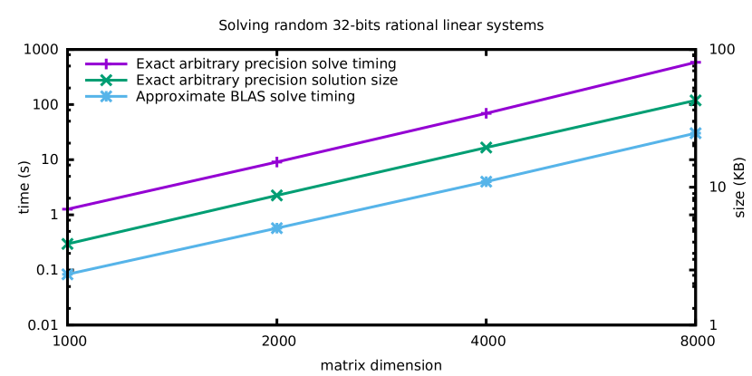
Figure 3: Comparison of approximate and arbitrary precision linear system solving on an Intel Xeon W3530 @2.80GHz.

We achieve good practical performance of computations in linear algebra by extensively applying reductions to MM, which we mostly perform exactly over small finite fields.

On the one hand, nowadays machine architecture, with their memory hierarchy, is also well-adapted to the highly homogeneous structure of the straightforward MM. This is true for numerical routines, where the stability issues have been worked out for fast MM in [16, 73, 50, 8]. This is also true for exact routines where, symmetrically, the costly reductions (modular or polynomial) have to be delayed as much as possible.

On the other hand, this straightforward algorithm remains faster in practice only for small matrices, but the larger memory capacity and the increase in the number of computing units makes it possible to handle, on desktop computers, dense matrices of dimensions in several hundred thousands. As the practical threshold between straightforward and fast algorithms is often for matrices of dimensions about 500, several fast routines can be very effectively combined, yielding the fastest implementations to date, as explained in the next section.

11.2 Design of fast exact matrix multiplication over word-size prime fields

The design of matrix multiplication routines over a word size finite field is the main building block for computations in exact dense linear algebra. In practice, a turning point has been the introduction of the following principles in [58]:

1. finite field arithmetic is reduced to integer arithmetic with delayed or simultaneous modular reductions;

2. integer arithmetic is performed by floating point units (in order to take advantage of SIMD instructions and of numerical routines development – BLAS);

3. computations are structured in blocks in order to optimize the use of the memory hierarchy of current architectures;

4. asymptotically fast algorithms are used, mostly recursive bilinear algorithm for MM based on Winograd’s $2\times 2$ MM of Example 2.2 (see also [52, 58, 28], hereafter we denote this algorithm WRB-MM), but also Kaporin’s [88] and Bini-Capovani-Lotti-Romani’s  [15, 26] algorithms are used.

The idea is to convert a finite field matrix into its integer representation, then perform the multiplication over the integers (potentially using, exactly, a floating point representation) and convert back the result into the finite field. First, a floating point representation allows us to use a sustainable code that rely on more widely supported numerical linear algebra routines. Further, on the one hand, machine division (for reductions) and integer units are slower than the respective floating point operations (for instance, not all integral operations have yet SIMD support [74]). But, on the other hand, as the computed results are exact, one can apply the fastest implementations of the asymptotically fast algorithms not worrying about numerical stability problems (which, even though never serious for fast MM, as this has been proved in [16, 50], can require some extra work).

Over finite fields, with arbitrary precision or with polynomials, it is nowadays much faster to perform additions or even multiplications than modular or polynomial reductions. To take the most of the machine representation, reduction is delayed or grouped using the following techniques:

Definition 11.1.

1. Delayed reduction is the action of replacing a classical dot product with reductions, $\sum_{i=0}^{n}Reduce(a_{i}b_{i})$, by an algorithm that reduces only from time to time, for instance, when the internal representation cannot hold the growth anymore:

   • Compute $s=\sum_{i=0}^{k}a_{i}b_{i}$; $Reduce(s)$;
     

   • For $j=1$ to $n/k-1$ compute
     

     $s=s+\sum_{i=jk+1}^{(j+1)k}a_{i}b_{i}$; $Reduce(s)$;
     

   • done;

2. Simultaneous modular reduction is the action of performing a single reduction on several coefficients at once: in other words, the idea is to replace independent reductions (for instance $Reduce(a)$;$Reduce(b)$;$Reduce(c)$) by a single reduction on grouped elements (use $t=Group(a,b,c)$;$Reduce(t)$;$a,b,c=Ungroup(t)$ instead), see, e.g., [56] for more details.

Moreover, in practice, for exact computations, recursion is important when fast algorithms are used: while tiling allows a static placement of blocks adapted to the memory hierarchy, larger blocks allow faster acceleration but also more delays in the application of reductions (modular reduction, polynomial reduction, etc.) [60]. Further, the fast algorithms can be used for a few levels of recursion and then switch back to the, statically placed, straightforward algorithm on smaller matrices. Eventually (nowadays, on a current personal computer, this can typically be between n=500 and n=1000), the exact algorithm sketched above is based on the numerical BLAS and then applied without any further recursion.

There is actually a cascade of algorithms where, at each recursive cutting, a new choice of the best suited variant is performed before the final switch [68, 27]. This cascade is usually non-stationary, i.e., a different scheme, bilinear or not, can be chosen at every level of recurrence. For instance, a meta-algorithm starts by partitioning the matrices into four blocks followed by application of WRB-MM. This meta-algorithm is called on each of the seven multiplications of the blocks; at the recursive call the meta-algorithm can decide whether to re-apply itself again to a $2\times 2$ block matrix or to switch either to a (2,2,3) APA algorithms (which in turns will also call this meta algorithm recursively) or to the straightforward algorithm, etc.

This impacts the frequency at which the modular reductions can be delayed. For instance, with a classical MM and elements of a prime field modulo $p>2$ represented as integers in $\{\frac{1-p}{2}\ldots\frac{p-1}{2}\}$, on a type with a mantissa of $m$ bits, the condition is that the modular reduction in a scalar product of dimension $k$ can be delayed to the end as long as $k\left(\frac{p-1}{2}\right)^{2}<2^{m}$.

When applying $\ell$ recursive levels of WRB-MM algorithm, it can be showed instead that some intermediate computations could grow above this bound [62], and the latter condition becomes $9^{\ell}\lfloor\frac{k}{2^{\ell}}\rfloor\left(\frac{p-1}{2}\right)^{2}<2^{m}$. This requires to perform by a factor of about $(9/2)^{\ell}$ more modular reductions.

Example of sequential speed obtained by the fgemm routine algorithm of the LinBox library [57] is shown in Table 11.1.

Table 11.1: Effective Gfops ($2n^{3}/time/10^{9}$) of matrix multiplications: LinBox fgemm vs OpenBLAS (s|d)gemm on one core of a Xeon E5-4620 @2.20GHz

$n$	1024	2048	4096	8192	16384
OpenBLAS sgemm	27.30	28.16	28.80	29.01	29.17
$\mathcal{O}\left(n^{3}\right)$-fgemm Mod 37	21.90	24.93	26.93	28.10	28.62
$\mathcal{O}\left(n^{2.81}\right)$-fgemm Mod 37	22.32	27.40	32.32	37.75	43.66
OpenBLAS dgemm	15.31	16.01	16.27	16.36	16.40
$\mathcal{O}\left(n^{3}\right)$-fgemm Mod 131071	15.69	16.20	16.40	16.43	16.47
$\mathcal{O}\left(n^{2.81}\right)$-fgemm Mod 131071	16.17	18.05	20.28	22.87	25.81

The efficiency of the fgemm routine is largely due to the efficiency of the BLAS, but as the latter are not using fast algorithms, exact computations can be faster. Modulo 37 elements are stored over single precision floats, and the sgemm subroutine can be used, whereas modulo 131071 elements are stored using double precision float, and the dgemm subroutine is used. Table 11.1 first shows that the overhead of performing the modular reductions in the $\mathcal{O}\left(n^{3}\right)$ implementations is very limited if the matrix is large enough. Then, when enabling WRB-MM $\mathcal{O}\left(n^{2.81}\right)$ algorithm, a speed-up of up to $40\%$ can be attained in both single and double precision arithmetic. More recently, it has been shown also how algorithm [15] by Bini et al. could be efficiently put into practice [26], also offering some interesting speed-up for prime fields of size near 10 bits.

11.3 Memory efficient schedules

WRB-MM algorithm requires external temporary memory allocations in order to store the intermediate linear combinations of blocks. With large matrices and current architectures, this can be penalizing because the memory availability and access to it dominate the overall computational costs. It is therefore crucial to reduce as much as possible the extra memory requirements of fast methods. This can be done via a careful scheduling of the steps of WRB-MM algorithm: it is not mandatory to perform 8 pre-additions, 7 multiplications and 7 post-additions in that order, with temporary memory allocations for each of these 22 steps. Depending on the associated dependency graph, one can choose instead to reduce the number of allocation by following this graph and overwriting already allocated memory when the associated variable is not used any more.

For the product of $n\times{}n$ matrices, without accumulation, $C\leftarrow{}A\times{}B$, [52] proposed a schedule requiring, apart from $C$, two extra temporary blocks of size $\frac{n}{2}\times\frac{n}{2}$ at the first recursive levels, two extra temporary blocks of size $\frac{n}{4}\times\frac{n}{4}$ for each of the seven recursive calls, etc. Overall, the needed extra memory is bounded by $\frac{2}{3}n^{2}$. For the product with accumulation, $C\leftarrow{}C+A\times{}B$, for more than ten years the record was three temporaries with an extra memory bounded by $n^{2}$ [81], but this was recently improved to two temporaries in [28]. Notice that [28] proposed also some schemes requiring smaller extra memory (that can actually be made quite close to zero), with the same asymptotic complexity as WRB-MM algorithm, although with a larger constant overhead factor in arithmetic operations. Recently M. Bodrato proposed a variant of WRB-MM algorithm, which is symmetric and more suitable to squaring matrices, but which uses similar schedules, and therefore keeps the extra requirements [22]. This is not the case in [80] where no extra memory is required if only one or two recursive levels of fast MM are used, but at the cost of recomputing many additions.

Finally, in the case of the APA algorithm [15] by Bini et al., the requirements are also of two temporaries in the product without accumulation [26]. From [81], new schedules have usually been discovered by hand, but with the help of a pebble game program, which discards rapidly the wrong schedules and verifies formally the correct ones.

11.4 Tiny finite fields

The practical efficiency of MM depends greatly on the representation of field elements. Thus we present three kinds of compact representations for the elements of a finite field with very small cardinality: bit-packing (for ${\mathbb{F}}_{2}$), bit-slicing (say, for ${\mathbb{F}}_{3},{\mathbb{F}}_{5},{\mathbb{F}}_{7},{\mathbb{F}}_{2^{3}}$, or ${\mathbb{F}}_{3^{2}}$), and Kronecker substitution. These representations are designed to allow efficient linear algebra operations, including MM:

Definition 11.2.

Compact representations for small finite fields.

1. Over ${\mathbb{F}}_{2}$, the method of the four Russians [7], also called Greasing, can be used as follows [2]:

   • A 64-bit machine word can be used in order to represent a row vector of dimension 64.

   • Multiplication of an $m\times k$ matrix $A$ by an $k\times n$ matrix $B$ can be done by first storing all $2^{k}$ $k$-dimensional linear combinations of rows of $B$ in a table. Then the $i$-th row of the product is copied from the row of the table indexed by the $i$-th row of $A$.

   • By ordering indices of the table according to a binary Gray Code, each row of the table can be deduced from the previous one, using only one row addition. This decreases the bit-operation count for building the table from $k2^{k}n$ to $2^{k}n$.

   • Choosing $k=\log_{2}n$ in this method implies $MM(n)=\mathcal{O}\left(n^{3}/\log n\right)$ over ${\mathbb{F}}_{2}$. In practice, the idea is once again to use a cascading algorithm: at first some recursive steps of fast MM is performed, and then, at a size small enough, one should switch to the greasing.

2. Bit-slicing consists in representing an $n$-dimensional vector of $k$-bit sized coefficients by using $k$ binary vectors of dimension $n$ [23]. In particular, one can apply Boolean word instruction in order to perform arithmetic on 64 dimensional vectors.

   • Over ${\mathbb{F}}_{3}$, the binary representation $0\equiv[0,0],1\equiv[1,0],-1\equiv[1,1]$ allows us to add and subtract two elements in 6 Boolean operations:

     $$\begin{array}[]{ll}\text{Add}([x_{0},x_{1}],[y_{0},y_{1}]):&s\leftarrow x_{0}\oplus y_{1},t\leftarrow x_{1}\oplus y_{0}\\ &\text{Return}(s\wedge t,(s\oplus x_{1})\vee(t\oplus y_{1}))\\ \text{Sub}([x_{0},x_{1}],[y_{0},y_{1}]):&t\leftarrow x_{0}\oplus y_{0}\\ &\text{Return}(t\vee(x_{1}\oplus y_{1}),(t\oplus y_{1})\wedge(y_{0}\oplus x_{1}))\end{array}$$

   • Over ${\mathbb{F}}_{5}$ (resp. ${\mathbb{F}}_{7}$), a redundant representation $x=x_{0}+2x_{1}+4x_{2}\equiv[x_{0},x_{1},x_{2}]$ allows us to add two elements by using 20 (resp. 17) Boolean operations, negate in 6 (resp. 3) Boolean operations, and double by using 5 (resp. 0) Boolean operations.

   Table 11.2: Boolean operation counts for basic arithmetic by using bit-slicing

   	${\mathbb{F}}_{3}$	${\mathbb{F}}_{5}$	$F_{7}$
   Addition	6	20	17
   Negation	1	6	3
   Double		5	0

3. Bit-packing consists in representing a vector of field elements as an integer that fits in a single machine word by using a $2^{k}$-adic representation:

   $$(x_{0},\dots,x_{n-1})\in{\mathbb{F}}_{q}^{n}\equiv X=x_{0}+2^{k}x_{1}+\dots+(2^{k})^{n-1}x_{n-1}\in\mathbb{Z}_{2^{64}}$$

   Elements of extension fields are viewed as polynomials and stored as the evaluation of this polynomial at the characteristic of the field. The latter evaluation is called Kronecker substitution [55]. Once we can pack and simultaneously reduce coefficients of the finite field in a single machine word, the obtained parallelism can be used for MM. Depending on the respective sizes of the matrices in the multiplication, one can pack only the left operand, only the right one, or both [56]. Then, over the field extensions, fast floating point operations can also be used on the Kronecker substitution of the elements.

All these methods improve in fact the base case of dense linear algebra, when fast methods are not competitive anymore. As already mentioned, the generic cascading idea applies: perform at first some recursive steps fast, decreasing the matrix dimension, and, at a small enough size, switch to the (improved) classical triple loop method.

11.5 Parallelization

Now, we focus on the design of a parallel MM routine, which computes the matrix product $AB$ based on the WRB-MM sequential algorithm. In order to parallelize the computation at the coarsest grain, the best approach is to apply first a classical block algorithm, generating a prescribed number of independent tasks, and then each of them will use the sequential WRB-MM algorithm [60, 59]. There, the parallel algorithm is recursive and splits the largest of either the row dimension of $A$ or the column dimension of $B$, to form two independent tasks. The granularity of the split is recursive and terminates whenever the number of created tasks becomes larger than the number of computing resources (e.g., the total number of cores). This maximizes the size of the blocks, and therefore the benefit of WRB-MM algorithm, while ensuring a large enough number of tasks for the computing resources.

Figure 4: Speed of exact and numerical matrix multiplication routines on a 32 cores Intel Xeon E5-4620 2.2Ghz (Sandy Bridge) with 16384KB L3 cache [59].

Figure 4 shows the computation time of various MM algorithms: the numerical dgemm implementation of Plasma-Quark, OpenBLAS and Intel-MKL as well as the implementation of pfgemm of LinBox using the OpenMP-4.0 data-flow model. Contrary to MKL, OpenBLAS or Plasma-Quark, this pfgemm routine uses the above sketched splitting strategy with WRB-MM. This implementation is run over the finite field $\mathbb{Z}/131071\mathbb{Z}$ or with real double floating point numbers. We first notice that most routines perform very similarly. More precisely, Intel-MKL dgemm is faster on small matrices, but the effect of WRB-MM algorithm makes pfgemm faster on larger matrices, even in the finite field where additional modular reductions occur.

12 Some Research Challenges

The field is still in progress, and here are some current observations.

(i) The implementations of fast trilinear aggregation algorithms by Kaporin in [87] and [88] are relatively little applied in practice so far, although they have important advantages versus other algorithms now in use: being at least as fast and more stable numerically and allowing highly efficient parallel implementation, they require much less memory. This is because the algorithms of [87] and [88] are defined by trilinear decompositions with supersparse coefficient matrices $A=(\alpha_{ij}^{(q)})_{(i,j),q}$, $B=(\beta_{jk}^{(q)})_{(j,k),q}$, and $C=(\gamma_{ik}^{(q)})_{(i,k),q}$ of (3.1), which is a general property of competently implemented trilinear aggregation algorithms. The implementations in [87] and [88] were intended to be initial rather than final steps and were supposed to leave some room for further amelioration. In particular the algorithm of [118], also relying on trilinear aggregation, has similar features, but supports even a smaller exponent, and can be a basis for further progress in the implementation of fast feasible MM.

(ii) The more recent algorithms of [136], obtained by means of computer search, are highly promising because they beat the exponent $\log_{2}(7)$ already for various small problems $MM(m,n,p)$ where $\min\{m,n,p\}=2$ and $\max\{m,n,p\}\leq 6$. Their coefficient matrices $A$, $B$, and $C$ of (3.1) are quite dense, however, and their tested performance is inferior to recursive bilinear algorithms based on Examples 2.2 and 2.3. This leads to the challenge of devising MM algorithms that would combine the best features of the algorithms of [87], [88], and [136].

(iii) Numerical instability of APA algorithms does not prevent them from being efficient in symbolic computations, but so far only the rudimentary algorithm of [15] has been implemented [26], while much simpler and much more efficient ones are ignored (cf., e.g., our algorithm in Section 7).

Some researchers in matrix computations still view decreasing the current record MM exponent of about 2.37 towards the lower bound 2 as the major theoretical challenge. For the state of affairs in this area we refer the reader to our Figure 2 and the mostly negative results in [4], [5], and [21].

We, however, consider breaking the barrier of 2.7733 for the realistic exponent of $MM(n)$, $n\leq 1,000,000$, a more important challenge. The exponent 2.773 stays unbeaten since 1982 (that is, longer than Coppersmith–Winograd’s barrier of 1986, broken by Stothers in 2010), and its decrease should require more powerful tools than the acceleration of infeasible MM because of the limitation on the use of recursive bilinear algorithms. We hope that this important challenge will be met in reasonable time, possibly based on combination of human ingenuity and computer search, and then significant impact on present day computations should be expected, whereas reaching the exponent 2 for MM of infeasible sizes per se would hardly make such an impact.

In view of microscopic progress in the decrease of the exponent of infeasible MM, the present day research directions towards that goal seem to lead to various dead ends, and any potential progress shall most likely rely on radically new insights, ideas and techniques, such as aggregation and mapping the input and output of MM to another dimension (cf. [112], [118], [119] and [94]).

In the area of the implementation of MM, further progress with recursive bilinear algorithms based on fast $2\times 2$ MM is a highly important challenge, and the recent advances by Bodrato [22] and Cenk and Hasan [36] are very encouraging, but it would greatly benefit the field if the researchers will not confine themselves to the geocentric viewpoint of 1969, restricted to $2\times 2$-based bilinear recursion, and will also explore heliocentric point of view of XXI century, by opening themselves to the benefits of trilinear world, aggregation, APA, and possibly some other new powerful Strassen-free techniques for fast feasible MM, yet to appear.

References

- [1] A.V. Aho, J.E. Hopcroft, J.D. Ullman, The Design and Analysis of Algorithms. Addison-Wesley, Reading, MA, 1974.
- [2] Martin R. Albrecht, Gregory V. Bard, and William Hart. Algorithm 898: Efficient multiplication of dense matrices over GF(2). ACM Trans. Math. Softw., 37(1), 2010. doi:10.1145/1644001.1644010.
- [3] N. Alon, Z. Galil, O. Margalit, On the Exponent of the All Pairs Shortest Path Problem, J. of Computer and System Sciences, 54, 2, 255–262. 1997.
- [4] N. Alon, A. Shpilka, C. Umans, On Sunflowers and Matrix Multiplication. Computational Complexity, 22, 2, 219–243, 2013.
- [5] A. Ambainis, Y. Filmus, F. Le Gall, Fast Matrix Multiplication: Limitations of the Laser Method. Electronic Colloquium on Computational Complexity (ECCC), year 2014, paper 154. http://eccc.hpi-web.de/report/2014/154. Available at arXiv:1411.5414, November 21, 2014.
- [6] R.R. Amossen, R. Pagh, Faster Join-projects and Sparse Matrix Multiplications. In Proceedings of the 12th International Conference on Database Theory, 121–126, 2009.
- [7] V. L. Arlazarov, E. A. Dinic, M. A. Kronrod, and I. A. Faradžev. The economical construction of the transitive closure of an oriented graph. Doklady Akademii Nauk SSSR, 194:487–488, 1970.
- [8] Ballard, G., Benson, A. R., Druinsky, A., Lipshitz, B., Schwartz, O., Improving the numerical stability of fast matrix multiplication algorithms, SIMAX, in print, and arXiv:1507.00687, 2015.
- [9] G. Ballard, E. Carson, J. Demmel, M. Hoemmen, N. Knight, O. Schwartz, Communication Lower Bounds and Optimal Algorithms for Numerical Linear Algebra. Acta Numerica, 23, 1–155, 2014.
- [10] G. Ballard, J. Demmel, O. Holtz, O. Schwartz, Graph expansion and communication costs of fast matrix multiplication, Journal of the ACM (JACM), 59, 6, Article No. 32 doi¿10.1145/2395116.2395121
- [11] G. Ballard, A. Druinsky, N. Knight, O. Schwartz, Hypergraph Partitioning for Sparse Matrix-Matrix Multiplication, arXiv:1603.05627.
- [12] D.H. Bayley, Extra High Speed Matrix Multiplication on the Cray-2. SIAM J. on Scientific and Statistical Computing, 9, 3, 603–607, 1988.
- [13] A.R. Benson, G. Ballard, A framework for practical parallel fast matrix multiplication. In Proceedings of the 20th ACM SIGPLAN Symposium on Principles and Practice of Parallel Programming, 42–53, ACM Press, New York, January 2015.
- [14] D. Bini, Relations Between Exact and Approximate Bilinear Algorithms: Applications. Calcolo, 17, 1, 87–97, 1980.
- [15] D. Bini, M. Capovani, G. Lotti, F. Romani, Complexity for Approximate Matrix Multiplication. Information Processing Letters, 8, 5, 234–235, June 1979.
- [16] D. Bini, G. Lotti, Stability of Fast Algorithms for Matrix Multiplication. Numerische Math., 36, 1, 63–72, 1980.
- [17] D. Bini, V.Y. Pan, Polynomial Division and Its Computational Complexity. J. Complexity, 2, 3, 179–203, 1986.
- [18] D. Bini, V.Y. Pan, Polynomial and Matrix Computations, Volume 1: Fundamental Algorithms. Birkhäuser, Boston, 1994.
- [19] M. Bläser, Lower Bounds for the Multiplicative Complexity of Matrix Multiplication. J. of Computational Complexity, 9, 2, 73–112, 2000.
- [20] M. Bläser, A -Lower Bound for the Multiplicative Complexity of Matrix Multiplication over Arbitrary Fields. Proc. 40th Ann. IEEE Symp. on Foundations of Computer Science (FOCS 1999), 45–50, IEEE Computer Society Press, Los Alamitos, CA 1999.
- [21] J. Blasiak, T. Church, H. Cohn, J. A. Grochow, E. Naslund, W. F. Sawin, C. Umans, On cap sets and the group-theoretic approach to matrix multiplication, arXiv:1605.06702, 2016.
- [22] Marco Bodrato. A Strassen-like matrix multiplication suited for squaring and higher power computation. In Proceedings of the 2010 International Symposium on Symbolic and Algebraic Computation, ISSAC ’10, pages 273–280, New York, NY, USA, 2010. ACM. doi:10.1145/1837934.1837987.
- [23] Thomas J. Boothby and Robert W. Bradshaw. Bitslicing and the method of four russians over larger finite fields, January 2009. arXiv:0901.1413.
- [24] A. Borodin, I. Munro, The Computational Complexity of Algebraic and Numeric Problems. American Elsevier, New York, 1975.
- [25] A. Bostan, C.-P. Jeannerod, E. Schost, Solving structured linear systems with large displacement rank. Theoretical Computer Science, 407, 1 3, 155 -181, 2008. Proceedings version in ISSAC’07, pp. 33 40, ACM Press, NY, 2007.
- [26] B. Boyer and J.-G. Dumas. Matrix multiplication over word-size modular fields using approximate formulae. ACM Transactions on Mathematical Software, 42(3):20.1–20.12, 2016. https://hal.archives-ouvertes.fr/hal-00987812.
- [27] B. Boyer, J.-G. Dumas, P. Giorgi, C. Pernet, and B. David Saunders. Elements of design for containers and solutions in the linbox library. In Hoon Hong and Chee Yap, editors, Mathematical Software - ICMS 2014, volume 8592 of Lecture Notes in Computer Science, pages 654–662. Springer Berlin Heidelberg, 2014. doi:10.1007/978-3-662-44199-2_98.
- [28] B. Boyer, J.-G. Dumas, C. Pernet, W. Zhou, Memory Efficient Scheduling of Strassen- Winograd’s Matrix Multiplication Algorithm. Proc. Intern. Symposium on Symbolic and Algebraic Computation (ISSAC 2009), 55–62, ACM Press, New York, 2009.
- [29] R.W. Brockett, D. Dobkin, On Optimal Evaluation of a Set of Bilinear Forms. Proc. of the 5th Annual Symposium on the Theory of Computing (STOC 1973), 88–95, ACM Press, New York, 1973.
- [30] R.W. Brockett, D. Dobkin, On the Number of Multiplications Required for a Matrix Multiplication. SIAM Journal on Computing, 5, 4, 624–628, 1976.
- [31] R.W. Brockett, D. Dobkin, On Optimal Evaluation of a Set of Bilinear Forms. Linear Algebra and Its Applications, 19, 3, 207–235, 1978.
- [32] N.H. Bshouty, A Lower Bound for Matrix Multiplication. SIAM J. on Computing, 18, 4, 759–765, 1989.
- [33] N.H. Bshouty, On the Additive Complexity of Matrix Multiplication, Information Processing Letters, 56, 6, 329–335, 1995.
- [34] J.R. Bunch, J.E. Hopcroft, Triangular Factorization and Inversion by Fast Matrix Multiplication. Mathematics of Computation, 28, 125, 231–236, 1974.
- [35] P. Bürgisser, M. Clausen, M.A. Shokrollahi, Algebraic Complexity Theory. Springer Verlag, 1997.
- [36] M. Cenk, M.A. Hasan. On the Arithmetic Complexity of Strassen-Like Matrix Multiplications. J. of Symbolic Computation, 2016, in press. doi: 10.1016/j.jsc.2016.07.004.
- [37] B.W. Char, K.O. Geddes, G.H. Gonnet, GCDHEU: Heuristic Polynomial GCD Algorithm Based on Integer GCD Computation. Proceedings of EUROSAM’84, Lecture Notes in Computer Science, 174, 285–296, Springer, New York, 1984.
- [38] H. Cohn, R. Kleinberg, B. Szegedy, C. Umans, Group-theoretic Algorithms for Matrix Multiplication. Proceedings of the 46th Annual Symposium on Foundations of Computer Science (FOCS 2005), (Pittsburgh, PA), 379–388, IEEE Computer Society Press, 2005.
- [39] H. Cohn, C. Umans, A Group-theoretic Approach to Fast Matrix Multiplication. Proceedings of the 44th Annual Symposium on Foundations of Computer Science (FOCS 2003), (Cambridge, MA), 438–449, IEEE Computer Society Press, 2003.
- [40] H. Cohn, C. Umans, Fast Matrix Multiplication Using Coherent Configurations. Proceedings of the 24th Annual ACM-SIAM Symposium on Discrete Algorithms (SODA 2013), 1074–1087, 2013.
- [41] D. Coppersmith, Rapid Multiplication of Rectangular Matrices. SIAM Journal on Computing, 11, 3, 467–471, 1982.
- [42] D. Coppersmith, Rectangular Matrix Multiplication Revisited. Journal of Complexity, 13, 1, 42–49, 1997.
- [43] D. Coppersmith, S. Winograd, On the Asymptotic Complexity of Matrix Multiplication. SIAM J. on Computing, 11, 3, 472–492, 1982. Proc. version in 23rd FOCS (Nashville, TN), 82–90, IEEE Computer Society Press, 1981.
- [44] D. Coppersmith, S. Winograd, Matrix Multiplicaton via Arithmetic Progressions. J. of Symbolic Computations, 9, 3, 251–280, 1990. Proc. version in 19th ACM Symposium on Theory of Computing (STOC 1987), (New York, NY), 1–6, ACM Press, New York, NY, 1987. Also Research Report RC 12104, IBM T.J. Watson Research Center, August 1986.
- [45] P. D’Alberto, A. Nicolau, Adaptive Winograd’s Matrix Multiplication. ACM Transactions on Mathematical Software, 36, 1, paper 3, 2009.
- [46] A.M. Davie, A.J. Stothers, Improved Bound for Complexity of Matrix Multiplication. Proceedings of the Royal Society of Edinburgh, 143A, 351–370, 2013.
- [47] H.F. de Groot, On Varieties of Optimal Algorithms for the Computation of Bilinear Mappings. Theoretical Computer Science, 7, 2, 127–148, 1978.
- [48] C. Demetrescu, G.F. Italiano, Fully Dynamic Transitive Closure: Breaking Through the Barrier. In Proceedings of the 41st Annual Symposium on Foundations of Computer Science (FOCS 2000), 381–389, 2000.
- [49] J. Demmel, I. Dumitriu, O. Holtz, Fast Linear Algebra Is Stable. Numerische Mathematik, 108, 1, 59–91, 2007.
- [50] J. Demmel, I. Dumitriu, O. Holtz, R. Kleinberg, Fast Matrix Multiplication Is Stable. Numerische Mathematik, 106, 2, 199–224, 2007.
- [51] John D. Dixon. Exact solution of linear equations using p-adic expansions. Numerische Mathematik, 40:137–141, 1982.
- [52] C.C. Douglas, M. Heroux, G. Slishman, R.M. Smith, GEMMW: A Portable Level 3 BLAS Winograd Variant Of Strassen’s Matrix-Matrix Multiply Algorithm. J. of Computational Physics, 110, 1, 1–10, 1994.
- [53] C.-E. Drevet, Md. N. Islam, É. Schost, Optimization Techniques for Small Matrix Multiplication. Theoretical Computer Science, 412, 22, 2219–2236, 2011.
- [54] R. Duan, S. Pettie, Fast Algorithms for Matrix Multiplication and Bottleneck Shortest Paths, Proceedings of the 15th Annual ACM-SIAM Symposium on Discrete Algorithms (SODA 2009), 384–391, 2009.
- [55] J.-G. Dumas. Q-adic transform revisited. In Proceedings of the 2008 International Symposium on Symbolic and Algebraic Computation, pages 63–69, New York, 2008. ACM. doi:10.1145/1390768.1390780.
- [56] J.-G. Dumas, Laurent Fousse, and Bruno Salvy. Simultaneous modular reduction and Kronecker substitution for small finite fields. Journal of Symbolic Computation, 46(7):823 – 840, 2011. Special Issue in Honour of Keith Geddes on his 60th Birthday. doi:10.1016/j.jsc.2010.08.015.
- [57] J.-G. Dumas, T. Gautier, M. Giesbrecht, P. Giorgi, B. Hovinen, E. Kaltofen, B. D. Saunders, W. J. Turner and G. Villard. LinBox: A Generic Library for Exact Linear Algebra. In ICMS’2002, Proceedings of the 2002 International Congress of Mathematical Software, pages 40–50, Beijing, China. http://ljk.imag.fr/membres/Jean-Guillaume.Dumas/Publications/icms.pdf.
- [58] J.-G. Dumas, T. Gautier, and C. Pernet. Finite field linear algebra subroutines. In Teo Mora, editor, ISSAC’2002, Proceedings of the 2002 ACM International Symposium on Symbolic and Algebraic Computation, Lille, France, pages 63–74. ACM Press, New York, July 2002. http://ljk.imag.fr/membres/J.-G..Dumas/Publications/Field_blas.pdf.
- [59] J.-G. Dumas, T. Gautier, C. Pernet, J.-L. Roch, and Z. Sultan. Recursion based parallelization of exact dense linear algebra routines for Gaussian elimination. Parallel Computing, 57:235–249, 2016. http://hal.archives-ouvertes.fr/hal-01084238.
- [60] J.-G. Dumas, T. Gautier, C. Pernet, and Z. Sultan. Parallel computation of echelon forms. In Euro-Par 2014, Proceedings of the 20th international conference on parallel processing, Porto, Portugal, volume 8632 of Lecture Notes in Computer Science, pages 499–510, August 2014. http://hal.archives-ouvertes.fr/hal-00947013.
- [61] J.-G. Dumas, P. Giorgi, C. Pernet, FFPACK: Finite Field Linear Algebra Package. Proc. Intern. Symposium on Symbolic and Algebraic Computation (ISSAC 2004), Jaime Gutierrez, editor, 119–126, ACM Press, New York, 2004.
- [62] J.-G. Dumas, P. Giorgi, and C. Pernet. Dense linear algebra over prime fields. ACM Transactions on Mathematical Software, 35(3):1–42, November 2008. http://hal.archives-ouvertes.fr/hal-00018223.
- [63] J.-G. Dumas and C. Pernet. Computational linear algebra over finite fields. In Daniel Panario and Gary L. Mullen, editors, Handbook of Finite Fields. Chapman & Hall/CRC, 2012. http://hal.archives-ouvertes.fr/hal-00688254.
- [64] J.-G. Dumas, C. Pernet, Z. Sultan, Fast Computation of the Rank Profile Matrix and the Generalized Bruhat Decomposition, J. of Symbolic Computation, 2016. Proc. version in ISSAC 2015.
- [65] C.M. Fiduccia, On Obtaining Upper Bound on the Complexity of Matrix Multiplication. In Analytical Complexity of Computations (edited by R.E. Miller, J. W. Thatcher, J. D. Bonlinger), in the the IBM Research Symposia Series, pp. 31–40, Plenum Press, NY, 1972.
- [66] C.M. Fiduccia, Polynomial Evaluation via the Division Algorithm: The Fast Fourier Transform Revisited. Proc. 4th Annual ACM Symposium on Theory of Computing (STOC 1972), 88–93, ACM Press, New York, 1972.
- [67] M.J. Fischer, M.S. Paterson, String-Matching and Other Products. SIAM–AMS Proc., 7, 113–125, 1974.
- [68] P.C. Fischer, Further Schemes for Combining Matrix Algorithms. Proceedings of the 2nd Colloquium on Automata, Languages and Programming, Lecture Notes in Computer Science, 14, 428–436, Springer-Verlag, London, UK, 1974.
- [69] M. Fürer, Faster Integer Multiplication. SIAM J. on Computing, 39, 3, 979–1005, 2009.
- [70] J. von zur Gathen, J. Gerhard (2013). Modern Computer Algebra. Cambridge University Press, Cambridge, UK, third edition, 2013.
- [71] G.H. Golub, C.F. Van Loan, Matrix Computations. Johns Hopkins University Press, Baltimore, Maryland, 2013 (4th addition).
- [72] L. Grasedyck, D. Kressner, C. Tobler, A Literature Survey of Low-rank Tensor Approximation Techniques. GAMM-Mitteilungen, 36, 1, 53–78, 2013.
- [73] N.J. Higham, Exploiting Fast Matrix Multiplication within Level 3 BLAS. ACM Trans. on Math. Software, 16, 4, 352–368, 1990.
- [74] Joris van der Hoeven, Grégoire Lecerf, and Guillaume Quintin. Modular SIMD arithmetic in mathemagix. ACM Transactions on Mathematical Software, 43(1):5, August 2016. arXiv:1407.3383.
- [75] J. W. Hong and H. T. Kung. I/O complexity: The red-blue pebble game. In Proc. 14th STOC, pages 326–333, New York, NY, USA, 1981. ACM. doi:10.1145_800076.802486.
- [76] J.E. Hopcroft, L.R. Kerr, Some Techniques for Proving Certain Simple Programs Optimal. Proceedings of the Tenth Annual Symposium on Switching and Automata Theory, 36–45, IEEE Computer Society Press, 1969.
- [77] J.E. Hopcroft, L.R. Kerr, On Minimizing the Number of Multiplications Necessary for Matrix Multiplication. SIAM J. on Applied Math., 20, 1, 30–36, 1971.
- [78] J.E. Hopcroft, J. Musinski, Duality Applied to Matrix Multiplication and Other Bilinear Forms. SIAM Journal on Computing, 2, 3, 159–173, 1973.
- [79] X. Huang, V.Y. Pan, Fast Rectangular Matrix Multiplication and Applications. Journal of Complexity, 14, 2, 257–299, 1998. Proc. version in Proc. Annual ACM International Symposium on Parallel Algebraic and Symbolic Computation (PASCO’97), 11–23, ACM Press, New York, 1997.
- [80] J. Huang, T.M. Smith, G.M. Henry, R.A. van de Geijn, Strassen’s Algorithm Reloaded. Proceedings of the International Conference for High Performance Computing, Networking, Storage and Analysis, SC ’16, 59:1–59:12, IEEE Press, Piscataway, NJ, USA, 2016. http://www.computer.org/csdl/proceedings/sc/2016/8815/00/8815a690.pdf
- [81] Steven Huss-Lederman, Elaine M. Jacobson, Jeremy R. Johnson, Anna Tsao, and Thomas Turnbull. Implementation of Strassen’s algorithm for matrix multiplication. In ACM, editor, Supercomputing ’96 Conference Proceedings: November 17–22, Pittsburgh, PA, New York, NY 10036, USA and 1109 Spring Street, Suite 300, Silver Spring, MD 20910, USA, 1996. ACM Press and IEEE Computer Society Press. doi:10.1145/369028.369096.
- [82] Oscar H. Ibarra, Shlomo Moran, and Roger Hui. A generalization of the fast LUP matrix decomposition algorithm and applications. Journal of Algorithms, 3(1):45–56, March 1982. doi:10.1016/0196-6774(82)90007-4.
- [83] C.-P. Jeannerod, C. Pernet, and A. Storjohann. Rank-profile revealing Gaussian elimination and the CUP matrix decomposition. Journal of Symbolic Computation, 56(0):46 – 68, 2013. doi:10.1016/j.jsc.2013.04.004.
- [84] R. W. Johnson, A. M. McLoughlin, Noncommutative Bilinear Algorithms for Matrix Multiplication, SIAM J. on Computing, 15, 2, 595–603, 1986.
- [85] E. Kaltofen and A. Storjohann. Encyclopedia of Applied and Computational Mathematics, Chapter “Complexity of computational problems in exact linear algebra”, 227–233. Springer, November 2015. doi:10.1007/978-3-540-70529-1_173.
- [86] H. Kaplan, M. Sharir, E. Verbin, Colored Intersection Searching via Sparse Rectangular Matrix Multiplication. In Proceedings of the 22nd ACM Symposium on Computational Geometry, 52–60, 2006.
- [87] I. Kaporin, A Practical Algorithm for Faster Matrix Multiplication. Numerical Linear Algebra with Applications, 6, 8, 687–700, 1999.
- [88] I. Kaporin, The Aggregation and Cancellation Techniques as a Practical Tool for Faster Matrix Multiplication. Theoretical Computer Science, 315, 2–3, 469–510, 2004.
- [89] S. Ke, B. Zeng, W. Han, V. Y. Pan, Fast Rectangular Matrix Multiplication and Some Applications. Science in China, Series A: Mathematics, 51, 3, 389–406, 2008.
- [90] Walter Keller-Gehrig. Fast algorithms for the characteristic polynomial. Theor. Comput. Sci., 36(2-3):309–317, June 1985. http://dl.acm.org/citation.cfm?id=3929.3939.
- [91] B.N. Khoromskij, Quantics Approximation of - Tensors in High-dimensional Numerical Modeling. Constructive Approximation, 34, 2, 257–280, 2011.
- [92] D.E. Knuth, The Art of Computer Programming: Volume 2, Seminumerical Algorithms. Addison-Wesley, Reading, Massachusetts, 1969 (first edition), 1981 (second edition), 1997 (third edition).
- [93] T.G. Kolda, B.W. Bader, Tensor Decompositions and Applications. SIAM Review, 51, 3, 455–500, 2009.
- [94] J. Laderman, V.Y. Pan, H.X. Sha, On Practical Algorithms for Accelerated Matrix Multiplication. Linear Algebra and Its Applications, 162–164, 557–588, 1992.
- [95] J.M. Landsberg, New Lower Bound for the Rank of Matrix Multiplication. SIAM J. on Computing, 43, 1, 144–149, 2014.
- [96] F. Le Gall, Faster Algorithms for Rectangular Matrix Multiplication. Proceedings of the 53rd Annual IEEE Symposium on Foundations of Computer Science (FOCS 2012), 514–523, IEEE Computer Society Press, 2012.
- [97] F. Le Gall, Powers of Tensors and Fast Matrix Multiplication. Proceedings of the 39th International Symposium on Symbolic and Algebraic Computation (ISSAC 2014), 296–303, ACM Press, New York, 2014.
- [98] L. Lee, Fast Context-free Grammar Parsing Requires Fast Boolean Matrix Multiplication. Journal of the ACM (JACM), 49, 1, 1–15, 2002.
- [99] G. Lotti, F. Romani, On the Asymptotic Complexity of Rectangular Matrix Multiplication. Theoretical Computer Science, 23, 171–185, 1983.
- [100] A. Massarenti, E. Raviolo, Corrigendum to ”The rank of matrix multiplication is at least ” [Linear Algebra and its Applications, 438, 11 (2013) 4500–4509]. Linear Algebra and its Applications, 445, 369–371, 2014.
- [101] W. L. Miranker, V. Y. Pan, Methods of Aggregations, Linear Algebra and Its Applications, 29, 231–257, 1980.
- [102] T.S. Motzkin, Evaluation of Polynomials and Evaluation of Rational Functions. Bull. of Amer. Math. Society, 61, 2, 163, 1955.
- [103] V. Neiger, Fast computation of shifted Popov forms of polynomial matrices via systems of modular polynomial equations. Proceedings of the International Symposium on Symbolic and Algebraic Computation (ISSAC’16), 365–372, ACM Press, New York, 2016.
- [104] A. Neumaier, D. Stehlé, Faster LLL-type reduction of lattice bases, Proceedings of the International Symposium on Symbolic and Algebraic Computation (ISSAC’16), 373–380, ACM Press, New York, 2016.
- [105] J.S.R. Nielsen, A. Storjohann, Algorithms for Simultaneous Padé Approximation, Proceedings of the International Symposium on Symbolic and Algebraic Computation (ISSAC’16), 405–412, ACM Press, New York, 2016.
- [106] I.V. Oseledets, Approximation of Matrices with Logarithmic Number of Parameters. Dokl. Math., 80, 2, 653–654, 2009.
- [107] I.V. Oseledets, Approximation of Matrices Using Tensor Decomposition. SIAM J. on Matrix Analysis and Applications, 31, 4, 2130–2145, 2010.
- [108] I.V. Oseledets, E.E. Tyrtyshnikov, TT-cross Approximation for Multidimensional Arrays. Linear Algebra Appls. 432, 1, 70–88, 2010.
- [109] I.V. Oseledets, E.E. Tyrtyshnikov, Algebraic Wavelet Transform via Quantics Tensor Train Decomposition. SIAM J. Scientific Computing, 33, 3, 1315–1328, 2011.
- [110] A.M. Ostrowski, On Two Problems in Absract Algebra Connected with Horner’s Rule. In the Studies Presented to R. von Mises, 40–48, Academic Press, New York, 1954.
- [111] V.Y. Pan, On Methods of Computing the Values of Polynomials. Uspekhi Matematicheskikh Nauk, 21, 1(127), 103–134, 1966. [Transl. Russian Mathematical Surveys, 21, 1(127), 105–137, 1966.]
- [112] V.Y. Pan, On Schemes for the Evaluation of Products and Inverses of Matrices (in Russian). Uspekhi Matematicheskikh Nauk, 27, 5 (167), 249–250, 1972.
- [113] V.Y. Pan, Strassen’s Algorithm Is Not Optimal. Trilinear Technique of Aggregating for Fast Matrix Multiplication. Proc. the 19th Annual IEEE Symposium on Foundations of Computer Science (FOCS’78), 166–176, IEEE Computer Society Press, Long Beach, California, 1978.
- [114] V.Y. Pan, Fields Extension and Trilinear Aggregating, Uniting and Canceling for the Acceleration of Matrix Multiplication. Proceedings of the 20th Annual IEEE Symposium on Foundations of Computer Science (FOCS’79), 28–38, IEEE Computer Society Press, Long Beach, California, 1979.
- [115] V.Y. Pan, New Fast Algorithms for Matrix Operations. SlAM J. on Computing, 9, 2, 321–342, 1980, and Research Report RC 7555, IBM T.J. Watson Research Center, February 1979.
- [116] V.Y. Pan, The Bit-Operation Complexity of the Convolution of Vectors and of the DFT. Technical report 80-6, Computer Science Dept., SUNY, Albany, NY, 1980. (Abstract in Bulletin of EATCS, 14, page 95, 1981.)
- [117] V.Y. Pan, New Combinations of Methods for the Acceleration of Matrix Multiplications. Computers and Mathematics (with Applications), 7, 1, 73–125, 1981.
- [118] V.Y. Pan, Trilinear Aggregating with Implicit Canceling for a New Acceleration of Matrix Multiplication. Computers and Mathematics (with Applications), 8, 1, 23–34, 1982.
- [119] V.Y. Pan, How Can We Speed up Matrix Multiplication? SIAM Review, 26, 3, 393–415, 1984.
- [120] V.Y. Pan, Trilinear Aggregating and the Recent Progress in the Asymptotic Acceleration of Matrix Operations. Theoretical Computer Science, 33, 1, 117–138, 1984.
- [121] V.Y. Pan, How to Multiply Matrices Faster. Lecture Notes in Computer Science, 179, Springer, Berlin, 1984.
- [122] V.Y. Pan, Better Late Than Never: Filling a Void in the History of Fast Matrix Multiplication and Tensor Decompositions, arXiv:1411.1972, November 2014.
- [123] V.Y. Pan, Matrix Multiplication, Trilinear Decompositions, APA Algorithms, and Summation, arXiv:1412.1145 CS, Submitted December 3, 2014, revised February 5, 2015.
- [124] C. Pernet. High Performance and Reliable Algebraic Computing. Habilitation à diriger des recherches, Université Joseph Fourier, Grenoble 1, November 2014. https://tel.archives-ouvertes.fr/tel-01094212.
- [125] C. Pernet, Computing with Quasiseparable Matrices, Proceedings of the International Symposium on Symbolic and Algebraic Computation (ISSAC’16), 389–396, ACM Press, New York, 2016.
- [126] C. Pernet and A. Storjohann. Faster algorithms for the characteristic polynomial. In Proceedings of the 2007 International Symposium on Symbolic and Algebraic Computation, ISSAC ’07, pages 307–314, New York, NY, USA, 2007. ACM. doi:10.1145/1277548.1277590.
- [127] R. L. Probert, On the Additive Complexity of Matrix Multiplication. SIAM J. on Computing, 5, 2, 187–203, 1976.
- [128] R.L. Probert, On the Complexity of Symmetric Computations. Canadian J. of Information Processing and Operational Res., 12, 1, 71–86, 1974.
- [129] R. Raz, A. Shpilka, Lower Bounds for Matrix Product, in Bounded Depth Circuits with Arbitrary Gates. SIAM J. on Computing, 32, 2, 488–513, 2003.
- [130] F. Romani, private communication at the Oberwolfach Conference in October of 1979.
- [131] F. Romani, Some Properties of Disjoint Sum of Tensors Related to MM. SIAM J. on Computing, 11, 2, 263–267, 1982.
- [132] P. Sankowski, M. Mucha, Fast Dynamic Transitive Closure with Lookahead. Algorithmica, 56, 2, 180–197, 2010.
- [133] A. Schönhage, Partial and Total Matrix Multiplication. SIAM J. on Computing, 10, 3, 434–455, 1981.
- [134] A. Schönhage, Asymptotically Fast Algorithms for the Numerical Multiplication and Division of Polynomials with Complex Coefficients. Proc. EUROCAM, Marseille (edited by J. Calmet), Lecture Notes in Computer Science 144, 3–15, Springer, Berlin, 1982.
- [135] A. Schönhage, V. Strassen, Schnelle Multiplikation großer Zahlen. Computing, 7, 3–4, 281–292, 1971.
- [136] A.V. Smirnov, The Bilinear Complexity and Practical Algorithms for Matrix Multiplication. Computational Mathematics and Mathematical Physics, 53, 12, 1781–1795 (Pleiades Publishing, Ltd), 2013. Original Russian Text in Zhurnal Vychislitel’noi Matematiki i Matematicheskoi Fiziki, 53, 12, 1970–1984, 2013.
- [137] A. Shpilka, Lower Bounds for Matrix Product. SIAM J. on Computing, 32, 5, 1185–1200, 2003.
- [138] A. Storjohann, On the complexity of inverting integer and polynomial matrices, Computational Complexity, 24, 777–821, 2015.
- [139] A. Storjohann. The shifted number system for fast linear algebra on integer matrices. Journal of Complexity, 21(4):609–650, 2005. doi:10.1016/j.jco.2005.04.002.
- [140] A. Storjohann, S. Yang, A relaxed algorithm for online matrix inversion, Proceedings of the International Symposium on Symbolic and Algebraic Computation (ISSAC’15), 339-346, ACM Press, New York, 2015.
- [141] A.J. Stothers, On the Complexity of Matrix Multiplication. Ph.D. Thesis, University of Edinburgh, 2010.
- [142] V. Strassen, Gaussian Elimination Is Not Optimal. Numerische Math., 13, 354–356, 1969.
- [143] V. Strassen, Evaluation of Rational Functions, in Analytical Complexity of Computations (edited by R.E. Miller, J. W. Thatcher, and J. D. Bonlinger), pages 1–10, Plenum Press, New York, 1972.
- [144] V. Strassen, Vermeidung von Divisionen. J. Reine Angew. Math., 1973, 264, 184–202, 1973.
- [145] V. Strassen, Some Results in Algebraic Complexity Theory, in Proceedings of the International Congress of Mathematicians, Vancouver, 1974 (Ralph D. James, editor), Volume 1, pages 497–501, Canadian Mathematical Society 1974.
- [146] V. Strassen, The Asymptotic Spectrum of Tensors and the Exponent of Matrix Multiplication. Proc. 27th Ann. Symposium on Foundation of Computer Science, 49–54, 1986.
- [147] J. Todd, Motivation for Working in Numerical Analysis. Communication on Pure and Applied Math., 8, 1, 97–116, 1955.
- [148] E.E. Tyrtyshnikov, Tensor Approximations of Matrices Generated by Asymptotically Smooth Functions. Mat. Sbornik, 194, 6, 147–160, 2003.
- [149] V. Vassilevska Williams, Multiplying Matrices Faster than Coppersmith–Winograd. Version available at http://theory.stanford.edu/virgi/matrixmult-f.pdf, retrieved on January 30, 2014. Also see Proc. 44th Annual ACM Symposium on Theory of Computing (STOC 2012), 887–898, ACM Press, New York, 2012.
- [150] A. Waksman, On Winograd’s Algorithm for Inner Products. IEEE Transactions on Computers, C-19, 4, 360–361, 1970.
- [151] S. Winograd, On the Number of Multiplications Required to Compute Certain Functions. Proc. of the National Academy of Sciences, 58, 5, 1840–1842, 1967.
- [152] S. Winograd, A New Algorithm for Inner Product. IEEE Transaction on Computers, C–17, 7, 693–694, 1968.
- [153] S. Winograd, On the Number of Multiplications Necessary to Compute Certain Functions. Communications on Pure and Applied Mathematics, 23, 2, 165–179, 1970.
- [154] S. Winograd, On Multiplication of Matrices. Linear Algebra and Its Applications, 4, 382–388, 1971.
- [155] S. Winograd, Arithmetic Complexity of Computations. CBMS-NSF Regional Conference Series in Applied Math., 33, SIAM, Philadelphia, 1980.
- [156] R. Yuster, Efficient Algorithms on Sets of Permutations, Dominance, and Real-weighted APSP Proceedings of the 15th Annual ACM-SIAM Symposium on Discrete Algorithms (SODA 2009), 384–391, 2009.
- [157] R. Yuster, U. Zwick, U. Detecting Short Directed Cycles Using Rectangular Matrix Multiplication and Dynamic Programming. In Proceedings of the 15th Annual ACM-SIAM Symposium on Discrete Algorithms (SODA 2004), 254–260, 2004.
- [158] R. Yuster, U. Zwick, Fast Sparse Matrix Multiplication. ACM Transactions on Algorithms, 1, 1, 2–13, 2005.
- [159] R. Yuster, U. Zwick, Answering Distance Queries in Directed Graphs Using Fast Matrix Multiplication. In Proceedings of 46th Annual IEEE Symposium on the Foundations of Computer Science (FOCS 2005), 389–396, IEEE Computer Society Press, 2005.
- [160] U. Zwick. All-pairs Shortest Paths Using Bridging Sets and Rectangular Matrix Multiplication. Journal of the ACM, 49, 3, 289–317, 2002.