Computing wedge probabilities

Abstract

A new formula for the probability that a standard Brownian motion stays between two linear boundaries is proved. A simple algorithm is deduced. Uniform precision estimates are computed. Different implementations have been made available online as R packages.

Keywords: Brownian motion; double boundary crossing; theta functions
MSC 2010: 60J65

1 Introduction

Let $W=\{W_{t}\,,\;t\geqslant 0\}$ be a standard Brownian motion defined on a filtered probability space $(\Omega,\mathcal{F},\mathbb{P})$. The probability that $W_{t}$ remains in the planar region between two linear boundaries $-a_{1}t-b_{1}$ and $a_{2}t+b_{2}$ will be referred to as wedge probability, and denoted by $k(a_{1},b_{1};a_{2},b_{2})$:

$$k(a_{1},b_{1};a_{2},b_{2})=\mathbb{P}[-a_{1}t-b_{1}\leqslant W_{t}\leqslant a_{2}t+b_{2}\,,\;\mbox{for all }t\geqslant 0]\;.$$ (1)

It is positive if and only if $a_{1},b_{1},a_{2},b_{2}$ are all positive, which will be assumed from now on. Doob [8] expressed $k(a_{1},b_{1};a_{2},b_{2})$ as the sum of a convergent series. Since then, Doob’s formula has been extended or applied by many authors, including [3, 10, 16, 4, 14, 23]. One reason for its success is that many boundary crossing problems reduce to computing a wedge probability, through the representation of a certain Gaussian process in terms of $W$ [19, 6]. The earliest example is the standard Brownian bridge:

$$\left\{B_{t},0\leqslant t<1\right\}\overset{d}{=}\left\{(1-t)W_{t/(1-t)},0\leqslant t<1\right\}\,.$$

From this representation one gets:

$$\mathbb{P}[\sup_{t\in[0,1]}|B_{t}|\leqslant a]=k(a,a;a,a)\;,$$ (2)

which is the the distribution function of the test statistic in the Kolmogorov-Smirnov two-sided test, computed by Kolmogorov [17]; see [24] for historical aspects. More generally, the probability that a (non necessarily standard) Brownian bridge stays between two linear segments is a wedge probability. This remark makes wedge probabilities a building block for more general boundary crossing problems, through the method of piecewise linear approximations. The exit probability of a stochastic process from a region of the plane limited by two curves is called Boundary Crossing Probability (BCP). Applications of BCP’s can be found in many fields, from non-parametric statistics to biology or finance: see [27] and references therein. Explicit results are scarse [15]. A general approximation method has been proposed by Wang and Potzelberger [26] for single boundaries and Novikov et al. [18] for double boundaries; see also [21, 7, 27]. The idea is to replace the two (nonlinear) boundaries by piecewise linear approximations. Given its two values at the bounds of an interval, the conditional distribution of $W$ is that of a Brownian bridge on that interval. Thus the probability that it stays between two linear segments is a wedge probability. Using the independent increment property of $W$, the probability that the standard Brownian motion stays between two piecewise linear boundaries is written as a multidimensional Gaussian integral, the integrand being a product of wedge probabilities [18, Theorem 1]. The integral can be approximated either as a Gauss-Hermite quadrature [13] or by a Monte Carlo method [20]. In both cases, the integrand must be repeatedly evaluated, which implies that many wedge probabilities must be calculated for very different sets of values. The problem is that in Doob’s formula, as well as in all other equivalent formulas published since, the speed of convergence of the series depends on the parameters, and may be very slow for small values. This makes the BCP approximation algorithms numerically unstable. The key to efficient computation of wedge probabilities has long been available: Jacobi’s theta functions and their double expression through Poisson’s summation formula. Kolmogorov [17] had already given two formulas for $k(a,a;a,a)$, and remarked the interest for numerical computation: one converges fast for relatively large values of $a$, the other for relatively small values. This is routinely used in statistical softwares implementing the Kolmogorov-Smirnov test. The connection of $k(a_{1},b_{1};a_{2},b_{2})$ with theta functions has been pointed out by Salminen and Yor [23]. However, no alternative to Doob’s formula has been deduced so far; this is the main contribution of this paper (Proposition 2.1). The algorithmic consequence is that computing at most three terms of the series either in Doob’s formula or in the new alternative suffices to approximate $k(a_{1},b_{1};a_{2},b_{2})$ with precision smaller than $10^{-16}$. Uniform bounds on precision and algorithmic consequences are presented in section 3. Several implementations are compared in section 4. An R package wedge has been made available online [9]. Its companion wedgeParallel permits full use of a multicore structure.

2 Alternative to Doob’s formula

Doob [8] (formula (4.3) p. 398) expresses $k(a_{1},b_{1};a_{2},b_{2})$ as follows:

$$k(a_{1},b_{1};a_{2},b_{2})=1-\sum_{n=1}^{+\infty}\mathrm{e}^{-2A_{n}}+\mathrm{e}^{-2B_{n}}-\mathrm{e}^{-2C_{n}}-\mathrm{e}^{-2D_{n}}\;,$$ (3)

with:

$$A_{n} = n^{2}a_{2}b_{2}+(n-1)^{2}a_{1}b_{1}+n(n-1)(a_{2}b_{1}+a_{1}b_{2})\;,$$

$$B_{n} = (n-1)^{2}a_{2}b_{2}+n^{2}a_{1}b_{1}+n(n-1)(a_{2}b_{1}+a_{1}b_{2})\;,$$

$$C_{n} = n^{2}(a_{1}b_{1}+a_{2}b_{2})+n(n-1)a_{2}b_{1}+n(n+1)a_{1}b_{2}\;,$$

$$D_{n} = n^{2}(a_{1}b_{1}+a_{2}b_{2})+n(n+1)a_{2}b_{1}+n(n-1)a_{1}b_{2}\;.$$

Here is another expression.

Proposition 2.1

For $a_{1},b_{1},a_{2},b_{2}>0$, denote:

$$a_{\pm}=\scriptstyle{\frac{a_{1}\pm a_{2}}{2}}\displaystyle{\,;\;b_{\pm}=}\scriptstyle{\frac{b_{1}\pm b_{2}}{2}}\displaystyle{\,;\;c=}\scriptstyle{\frac{a_{1}b_{1}-a_{2}b_{2}}{2}}\displaystyle{\,;\;d=}\scriptstyle{\frac{a_{1}b_{2}-a_{2}b_{1}}{2}}\displaystyle{\;.}$$

Then:

$$\begin{array}[]{rl}\displaystyle{k(a_{1},b_{1};a_{2},b_{2})=}\scriptstyle{\sqrt{\frac{\pi}{2a_{+}b_{+}}}}\displaystyle{\,\mathrm{e}^{\frac{d^{2}}{2a_{+}b_{+}}}\sum_{n=1}^{+\infty}}&\displaystyle{\Big{(}\mathrm{e}^{-\frac{\pi^{2}(2n)^{2}}{8a_{+}b_{+}}}\big{(}\cos(\scriptstyle{\frac{\pi(2n)d}{2a_{+}b_{+}}}\displaystyle{)-\cos(}\scriptstyle{\frac{\pi(2n)c}{2a_{+}b_{+}}}\displaystyle{)\big{)}}}\\ &\displaystyle{+\mathrm{e}^{-\frac{\pi^{2}(2n-1)^{2}}{8a_{+}b_{+}}}\big{(}\cos(\scriptstyle{\frac{\pi(2n-1)d}{2a_{+}b_{+}}}\displaystyle{)+\cos(}\scriptstyle{\frac{\pi(2n-1)c}{2a_{+}b_{+}}}\displaystyle{)\big{)}\Big{)}\;.}}\end{array}$$ (4)

Proof: In terms of $a_{\pm}$, $b_{\pm}$, $c$, $d$, the expressions of $A_{n}$, $B_{n}$, $C_{n}$, $D_{n}$ are:

$$A_{n} = (2n-1)^{2}a_{+}b_{+}-(2n-1)c+a_{-}b_{-}\;,$$

$$B_{n} = (2n-1)^{2}a_{+}b_{+}+(2n-1)c+a_{-}b_{-}\;,$$

$$C_{n} = (2n)^{2}a_{+}b_{+}+2nd\;,$$

$$D_{n} = (2n)^{2}a_{+}b_{+}-2nd\;.$$

Hence:

$$\begin{array}[]{rl}\displaystyle{k(a_{1},b_{1};a_{2},b_{2})=1+2\sum_{n=1}^{+\infty}}&\displaystyle{\Big{(}\mathrm{e}^{-2(2n)^{2}a_{+}b_{+}}\cosh(2(2n)d)}\\ &\displaystyle{-\mathrm{e}^{-2a_{-}b_{-}}\mathrm{e}^{-2(2n-1)^{2}a_{+}b_{+}}\cosh(2(2n-1)c)\Big{)}\;.}\end{array}$$ (5)

Not meaning to add anything to the “bewildering variety of notations” for theta functions [1, p. 576], let us denote by $\theta$ the following function of two complex variables:

$$\theta(u,v)=\sum_{n=-\infty}^{+\infty}\mathrm{e}^{-2n^{2}u}\cosh(2nv)\;.$$ (6)

Observe that:

$$\theta(u,v+\scriptstyle{\frac{\mathrm{i}\pi}{2}}\displaystyle{)}=\sum_{n=-\infty}^{+\infty}(-1)^{n}\mathrm{e}^{-2n^{2}u}\cosh(2nv)\;.$$ (7)

By Poisson’s summation formula (see for instance formula (11) p. 236 of [25]), one gets:

$$\theta(u,v)=\sqrt{\frac{\pi}{2u}}\,\mathrm{e}^{v^{2}/(2u)}\sum_{n=-\infty}^{+\infty}\mathrm{e}^{-\pi^{2}n^{2}/(2u)}\cos(\pi nv/u)\;,$$ (8)

and:

$$\theta(u,v+\scriptstyle{\frac{\mathrm{i}\pi}{2}}\displaystyle{)}=\sqrt{\frac{\pi}{2u}}\,\mathrm{e}^{v^{2}/(2u)}\sum_{n=-\infty}^{+\infty}\mathrm{e}^{-\pi^{2}(n+\frac{1}{2})^{2}/(2u)}\cos(\pi(n+\scriptstyle{\frac{1}{2}}\displaystyle{)v/u)\;.}$$ (9)

From (5), (6), and (7):

$$k(a_{1},b_{1};a_{2},b_{2}) = \frac{1}{2}\big{(}\theta(a_{+}b_{+},d)+\theta(a_{+}b_{+},d+\scriptstyle{\frac{\mathrm{i}\pi}{2}}\displaystyle{)}\big{)}$$

$$-\frac{\mathrm{e}^{-2a_{-}b_{-}}}{2}\big{(}\theta(a_{+}b_{+},c)-\theta(a_{+}b_{+},c+\scriptstyle{\frac{\mathrm{i}\pi}{2}}\displaystyle{)}\big{)}\;.$$

Combining four evaluations of $\theta$ does not quite solve the numerical problem for small values of $a_{+}b_{+}$. The terms of the four series need further rearrangement. It is obtained observing that:

$$c^{2}-4a_{-}b_{-}a_{+}b_{+}=d^{2}\;.$$

Hence:

$$\mathrm{e}^{-2a_{-}b_{-}}\mathrm{e}^{\frac{c^{2}}{2a_{+}b_{+}}}=\mathrm{e}^{\frac{d^{2}}{2a_{+}b_{+}}}\;.$$

From there, (4) follows. $\square$ As remarked by Salminen and Yor [23], the symmetry and scaling properties of $k$ can be read on Doob’s formula. They also appear on (4):

$$k(a_{1},b_{1};a_{2},b_{2})=k(a_{2},b_{2};a_{1},b_{1})=k(b_{1},a_{1};b_{2},a_{2})=k(\frac{a_{1}}{u},ub_{1};\frac{a_{2}}{u},ub_{2})\;.$$

When slopes or intercepts are equal the expressions are simpler. If $a_{1}=a_{2}=a$ then $a_{+}=a$, $a_{-}=0$, $c=-d=ab_{-}$, and:

$$k(a,b_{1};a,b_{2}) = 1+2\sum_{n=1}^{+\infty}(-1)^{n}\mathrm{e}^{-2n^{2}ab_{+}}\cosh(2nab_{-})$$

$$= \sqrt{\frac{2\pi}{ab_{+}}}\mathrm{e}^{\frac{ab_{-}^{2}}{2b_{+}}}\sum_{n=1}^{+\infty}\mathrm{e}^{-\frac{\pi^{2}(2n-1)^{2}}{8ab_{+}}}\cos(\pi(2n-1)\scriptstyle{\frac{b_{-}}{2b_{+}}}\displaystyle{))\;.}$$

When both slopes and intercepts are equal one gets:

$$k(a,b;a,b) = 1+2\sum_{n=1}^{+\infty}(-1)^{n}\mathrm{e}^{-2n^{2}ab}$$

$$= \sqrt{\frac{2\pi}{ab}}\sum_{n=1}^{+\infty}\mathrm{e}^{-\frac{\pi^{2}(2n-1)^{2}}{8ab}}\;.$$

The first sum is formula (4.3’) of [8]. When slopes equal intercepts, the probability for a standard Brownian bridge to stay in a horizontal band is obtained, i.e. formula (4.9) p. 448 of [5]. If $b_{1}=a_{1}$ and $b_{2}=a_{2}$, then $b_{\pm}=a_{\pm}$, $c=2a_{+}a_{-}$, $d=0$, and:

$$k(a_{1},a_{1};a_{2},a_{2}) = 1+\sum_{n=1}^{+\infty}2\mathrm{e}^{-2(n(a_{1}+a_{2}))^{2}}-\mathrm{e}^{-(2n(a_{1}+a_{2})-a_{1})^{2}}-\mathrm{e}^{-(2n(a_{1}+a_{2})-a_{2})^{2}}$$

$$= \sqrt{\frac{\pi}{2}}\frac{1}{a_{+}}\sum_{n=1}^{+\infty}\mathrm{e}^{-\frac{\pi^{2}(2n)^{2}}{8a_{+}^{2}}}(1-\cos(\pi(2n)\scriptstyle{\frac{a_{-}}{a_{+}}}\displaystyle{))}$$

$$\hskip 45.52458pt+\mathrm{e}^{-\frac{\pi^{2}(2n-1)^{2}}{8a_{+}^{2}}}(1+\cos(\pi(2n-1)\scriptstyle{\frac{a_{-}}{a_{+}}}\displaystyle{))\;.}$$

Finally, the case where all four parameters are equal is the probability for a standard Brownian bridge to stay in a horizontal band centered at $0$, i.e. the distribution function of the test statistic in the Kolmogorov-Smirnov two-sided test. The formulas were originally found by Kolmogorov [17]; Feller [12] gave a simpler proof. Both had remarked the double expression coming from theta functions, and its interest for numerical computation.

$$k(a,a;a,a) = 1+2\sum_{n=1}^{+\infty}(-1)^{n}\mathrm{e}^{-2n^{2}a^{2}}$$

$$= \frac{\sqrt{2\pi}}{a}\sum_{n=1}^{+\infty}\mathrm{e}^{-\frac{\pi^{2}(2n-1)^{2}}{8a^{2}}}\;.$$

3 Algorithm and precision

Denote by $K_{1,N}$ and $K_{2,N}$ the partial sums up to $N$ in formulas (3) and (4).

$$K_{1,N}=1-\sum_{n=1}^{N}\mathrm{e}^{-2A_{n}}+\mathrm{e}^{-2B_{n}}-\mathrm{e}^{-2C_{n}}-\mathrm{e}^{-2D_{n}}\;,$$ (10)

$$\begin{array}[]{rl}\displaystyle{K_{2,N}=\sqrt{\frac{\pi}{2a_{+}b_{+}}}\,\mathrm{e}^{\frac{d^{2}}{2a_{+}b_{+}}}\sum_{n=1}^{N}}&\displaystyle{\Big{(}\mathrm{e}^{-\frac{\pi^{2}(2n)^{2}}{8a_{+}b_{+}}}\big{(}\cos(\scriptstyle{\frac{\pi(2n)d}{2a_{+}b_{+}}}\displaystyle{)-\cos(}\scriptstyle{\frac{\pi(2n)c}{2a_{+}b_{+}}}\displaystyle{)\big{)}}}\\ &\displaystyle{+\mathrm{e}^{-\frac{\pi^{2}(2n-1)^{2}}{8a_{+}b_{+}}}\big{(}\cos(\scriptstyle{\frac{\pi(2n-1)d}{2a_{+}b_{+}}}\displaystyle{)+\cos(}\scriptstyle{\frac{\pi(2n-1)c}{2a_{+}b_{+}}}\displaystyle{)\big{)}\Big{)}\;.}}\end{array}$$ (11)

The question is: for a given set of parameters $a_{1},b_{1},a_{2},b_{2}$, which of $K_{1,N}$ and $K_{2,N}$ should be computed, and which value of $N$ ensures a given precision? Proposition 3.1 bounds remainders.

Proposition 3.1

Denote by $R_{1,N}$ and $R_{2,N}$ the remainders:

$$R_{1,N}=K_{1,\infty}-K_{1,N}\quad\mbox{and}\quad R_{2,N}=K_{2,\infty}-K_{2,N}\;.$$

For $N>1$:

$$R_{1,N}\leqslant\scriptstyle{\frac{1}{4a_{+}b_{+}(N-1)}}\displaystyle{\mathrm{e}^{-8a_{+}b_{+}(N-1)^{2}}\;,}$$ (12)

$$R_{2,N}\leqslant\scriptstyle{\left(\frac{2}{\pi}\right)^{3/2}\frac{\sqrt{a_{+}b_{+}}}{N}}\displaystyle{\mathrm{e}^{2a_{+}b_{+}}\mathrm{e}^{-\frac{\pi^{2}N^{2}}{2a_{+}b_{+}}}\;.}$$ (13)

Proof: For both bounds, the following well known inequality is used: for any positive $u$,

$$\sum_{n=N+1}^{+\infty}\mathrm{e}^{-un^{2}}\leqslant\frac{\mathrm{e}^{-uN^{2}}}{2uN}\;.$$ (14)

In $R_{1,N}$, all four terms $A_{n}$, $B_{n}$, $C_{n}$, $D_{n}$ are larger than $4(n-1)^{2}a_{+}b_{+}$. Hence:

$$R_{1,N}\leqslant 4\sum_{n=N+1}^{+\infty}\mathrm{e}^{-8(n-1)^{2}a_{+}b_{+}}\;,$$

from where (12) follows by (14). For $R_{2,N}$, notice first that $|d|\leqslant 2\sqrt{a_{+}b_{+}}$, by Schwarz inequality. Hence:

$$R_{2,N} \leqslant \sqrt{\frac{2\pi}{a_{+}b_{+}}}\mathrm{e}^{2a_{+}b_{+}}\sum_{n=N+1}^{+\infty}\mathrm{e}^{-\frac{\pi^{2}(2n)^{2}}{8a_{+}b_{+}}}+\mathrm{e}^{-\frac{\pi^{2}(2n-1)^{2}}{8a_{+}b_{+}}}$$

$$= \sqrt{\frac{2\pi}{a_{+}b_{+}}}\mathrm{e}^{2a_{+}b_{+}}\sum_{n=2N+1}^{+\infty}\mathrm{e}^{-\frac{\pi^{2}n^{2}}{8a_{+}b_{+}}}\;.$$

Using again (14) leads to (13). $\square$ As expected, the bound on $R_{1,N}$ decreases with $a_{+}b_{+}$, the bound on $R_{2,N}$ increases. Denote by $\tau_{N}$ the value of $a_{+}b_{+}$ such that both bounds are equal, and by $\varepsilon_{N}$ their common value. Computing $K_{1,N}$ if $a_{+}b_{+}\geqslant\tau_{N}$ and $K_{2,N}$ else ensures $\varepsilon_{N}$ precision at least, whatever $a_{1},b_{1},a_{2},b_{2}$. The values of $\tau_{N}$ and $\varepsilon_{N}$ for $N=2,\ldots,8$ are given in Table 1.

$N$ $2$ $3$ $4$ $5$ $6$ $7$ $8$ $\tau_{N}$ $1.380$ $1.136$ $1.030$ $0.973$ $0.937$ $0.912$ $0.895$ $\varepsilon_{N}$ $\scriptstyle{2.9~{}10^{-6}}$ $\scriptstyle{1.8~{}10^{-17}}$ $\scriptstyle{5.1~{}10^{-34}}$ $\scriptstyle{5.6~{}10^{-56}}$ $\scriptstyle{2.3~{}10^{-83}}$ $\scriptstyle{3.5~{}10^{-116}}$ $\scriptstyle{1.9~{}10^{-154}}$

Table 1: Threshold and precision per number of terms computed.

In particular, for $N=3$ a precision $\varepsilon_{3}=1.8~{}10^{-17}$ is obtained, which is below current machine double precision. Thus $N=3$ was chosen as default value in our implementation. Computing more than two terms is usually not necessary. To illustrate this a Monte Carlo study has been conducted, over $10^{6}$ four-tuples of independent random values drawn in the interval $[0{,}10]$ with cumulative distribution function $(x/10)^{1/2}$. That choice ensured that wedge probabilities covered the whole range of $[0,1]$, with higher mass on values close to $0$ or $1$. For both sums the number of terms to convergence was defined as the first value of $N$ such that the remainder is smaller than $\varepsilon=10^{-16}$. As predicted by Proposition 3.1, in all $10^{6}$ cases either $K_{1,N}$ or $K_{2,N}$ reached $\varepsilon$ precision with $N=3$ terms or less. Actually, in $2.5\%$ of the cases, the result was smaller than $\varepsilon$ or larger than $1-\varepsilon$: no summation was needed. In $73.8\%$ of the cases $N=1$ sufficed to get $\varepsilon$ precision, and in $20.6\%$ of the cases $N=2$ terms were necessary; only in $0.56\%$ of the cases were $N=3$ terms necessary. Experimental results evidenced the need for an alternative to $K_{1,N}$. Indeed, in $442$ out of the $10^{6}$ cases, the number of terms to convergence of $K_{1,N}$ was larger than $100$, and in $1558$ cases it was larger than $50$. Figure 1 presents the numbers of terms to convergence as a function of $\log(a_{+}b_{+})$, for all $10^{6}$ random values, and both $K_{1,N}$ and $K_{2,N}$. As expected, the numbers decrease for $K_{1,N}$; they increase for $K_{2,N}$.

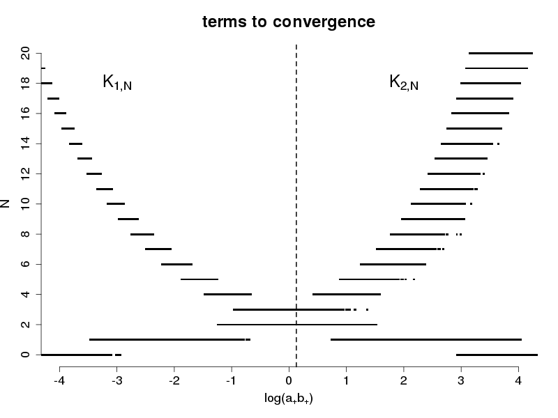
Figure 1: Number of terms to convergence as a function of $\log(a_{+}b_{+})$ for $K_{1,N}$ and $K_{2,N}$, over $10^{6}$ simulated values of $a_{1},b_{1};a_{2},b_{2}$. The dashed vertical line marks the theoretical threshold for $N=3$ i.e. $\tau_{3}=1.136$.

4 Implementation

The calculation of successive terms in $K_{1,N}$ or $K_{2,N}$ is easily vectorized. This makes the computation of a vector of wedge probabilities relatively fast in pure R [22]. Our objective was to explore gains in computing time, using existing R tools. The most widely used of these tools is Rcpp [11]. It uses (usually faster) compiled C++ code, interfaced with the R environment. Most computers now have a multicore architecture. However by default, both R or Rcpp use only one core. Taking full advantage of a multicore stucture can be done for example through RcppParallel [2].

Numerical experiments have been made using vectors of simulated entries with the same distribution as in section 3: independent entries on $[0{,}10]$ with cumulative distribution function $(x/10)^{1/2}$. Five implementations were considered: pure R, one-core Rcpp, RcppParallel with 4, 6, and 8 cores. Table 2 reports running times on a MacBookPro Retina 15. The running time for $10^{6}$ values in pure R ($0.725$ second), can be considered satisfactory. However, the gain in time goes up to twentyfold if an eight-core architecture is used. One of the known limitations of vectorized versions in pure R is memory space: ours cannot deal with vectors larger than $10^{7}$ entries.

$n$ R Rcpp RcppParallel (4) RcppParallel (6) RcppParallel (8) $10^{6}$ 0.725 0.169 0.05 0.044 0.036 $10^{7}$ 5.854 1.785 0.471 0.417 0.353 $10^{8}$ — 17.607 4.725 4.266 3.987

Table 2: Times in second for calculating wedge probabilities over vectors of size $n=10^{6},10^{7},10^{8}$, in pure R, Rcpp, RcppParallel with 4, 6, 8 threads. For $n=10^{8}$, calculations exceed memory space in pure R.

An R package wedge has been made available online [9]. In order to address installation issues for users not interested by a parallel version, the companion package wedgeParallel has been left as an option.

References

- [1] M. Abramowitz and I. A. Stegun. Handbook of mathematical functions with formulas, graphs, and mathematical tables, volume 55 of National Bureau of Standards Applied Mathematics Series. Courier Corporation, Washington D.C., 1964.
- [2] J.J. Allaire, R. François, K. Ushey, G. Vandenbrouck, M. Geelnard, and Intel. RcppParallel: Parallel Programming Tools for ’Rcpp’, 2016. R package version 4.3.20.
- [3] T. W. Anderson. A modification of the sequential probability ratio test to reduce the sample size. Ann. Math. Statist., 31(1):165–197, 1960.
- [4] L. Barba Escriba. A stopped Brownian motion formula with two sloping line boundaries. Ann. Probab., 15(4):1524–1526, 1987.
- [5] P. Biane, J. Pitman, and M. Yor. Probability laws related to he Jacobi theta and Riemann zeta functions, and Brownian excursions. Bull. Amer. Math. Soc., 38(4):435–465, 2001.
- [6] A. N. Borodin and P. Salminen. Handbook of Brownian motion – Facts and formulae. Birkhäuser, Basel, 2nd edition, 2002.
- [7] K. Borovkov and A. Novikov. Explicit bounds for appproximation rates of boundary crossing probabilities for the Wiener process. J. Appl. Probab., 42(1):85–92, 2005.
- [8] J. L. Doob. Heuristic approach to the Kolmogorov-Smirnov theorems. Ann. Math. Statist., 20(3):393–403, 1949.
- [9] R. Drouilhet and B. Ycart. wedge: an R package for computing wedge probabilities, 2016. http://github.com/rcqls/wedge
- [10] J. Durbin. Boundary-crossing probabilities for the Brownian motion and Poisson processes and techniques for computing the power of the Kolmogorov-Smirnov test. J. Appl. Probab., 8(3):431–453, 1971.
- [11] D. Eddelbuettel. Seamless R and C++ Integration with Rcpp. Springer, New York, 2013. ISBN 978-1-4614-6867-7.
- [12] W. Feller. On the Kolmogorov-Smirnov limit theorems for empirical distributions. Ann. Math. Statist., 19(2):177–189, 1948.
- [13] A. Genz and F. Bretz. Computation of multivariate normal and probabilities. Number 195 in L. N. Statist. Springer, New York, 2009.
- [14] W. J. Hall. The distribution of Brownian motion on linear crossing boundaries. Sequential Anal., 16:345–352, 1997.
- [15] N. Kahale. Analytic crossing probabilities for certain barriers by Brownian motion. Ann. Appl. Probab., 18(4):1424–1440, 2008.
- [16] D. P. Kennedy. Limit theorems for finite dams. Stoch. Proc. Appl., 1(3):269–278, 1973.
- [17] A. N. Kolmogorov. Sulla determinazione empirica di una legge di distribuzione. Giorn. Ist. Ital. Attuari, 4:83–91, 1933.
- [18] A. Novikov, V. Frishling, and N. Korzakhia. Approximations of boundary crossing probabilities for a Brownian motion. J. Appl. Probab., 36(4):1019–1030, 1999.
- [19] C. Park. Representations of Gaussian processes by Wiener processes. Pacific J. Math., 94(2):407–415, 1981.
- [20] K. Pötzelberger. Improving the Monte Carlo estimation of boundary crossing probabilities by control variables. Monte Carlo Methods Appl., 18(4):353–377, 2012.
- [21] K. Pötzelberger and L. Wang. Boundary crossing probability for Brownian motion. J. Appl. Probab., 38(1):152–164, 2001.
- [22] R Development Core Team. R: A Language and Environment for Statistical Computing. R Foundation for Statistical Computing, Vienna, Austria, 2008. ISBN 3-900051-07-0.
- [23] P. Salminen and M. Yor. On hitting times of affine boundaries by reflecting Brownian motion and Bessel processes. Period. Math. Hungarica, 62(1):75–101, 2011.
- [24] M. A. Stephens. Introduction to Kolmogorov (1933) On the Empirical Determination of a Distribution. In S. Kotz and N. L. Johnson, editors, Breakthroughs in Statistics, volume II of Springer Series in Statistics, pages 93–105. Springer, New York, 1992.
- [25] B. van der Pol and H. Bremmer. Operational calculus based on the two-sided Laplace integral. Cambridge University Press, Cambridge, 1950.
- [26] L. Wang and K. Pötzelberger. Boundary crossing probability for Brownian motion and general boundary. J. Appl. Probab., 34(1):54–65, 1997.
- [27] L. Wang and K. Pötzelberger. Crossing probabilities for diffusion processes with piecewise continuous boundaries. Methodol. Comput. Appl. Probab., 9:21–40, 2007.