Gas pressure in bubble attached to tube circular outlet

¹ Université Paris-Sud, Laboratoire de Physique des Solides, UMR8502, Orsay, F-91405

² Université Paris Diderot–Paris 7 Matière et Systèmes Complexes (CNRS UMR 7057), Bâtiment Condorcet, Case courrier 7056, 75205 Paris Cedex 13

³ Present address: Biological and Soft Systems, University of Cambridge, UK.

In the present Supplementary notes to our work “Arresting bubble coarsening: A two-bubble experiment to investigate grain growth in presence of surface elasticity” (submitted to EPL), we derive the expression of the gas pressure $p_{\rm gas}$ inside a bubble of volume $V$ located above and attached to the outlet of a tube of radius $r_{\rm out}$ (see Fig. 1a):

$$p_{\rm gas} \approx p_{\rm liq}^{\rm out}+2\frac{\gamma}{R}-\frac{4}{3}\rho gR$$ (1)

where $p_{\rm liq}^{\rm out}$ is the pressure in the liquid at the same altitude as the tube outlet (see Fig. 1a) and where $R$ is defined from the bubble volume $V$ as the radius of a sphere of volume $V$:

$$R = \left(\frac{3V}{4\pi}\right)^{1/3}$$ (2)

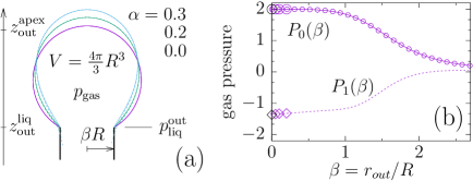
Figure 1: Left: Numerical simulation of the shape of a bubble of volume $4\pi R^{3}/3$ attached to an outlet of radius $r_{\rm out}=\beta R$, with different intensities of gravity (parameter $\alpha$). Exact shapes are plotted as solid lines. The shapes obtained at first order in $\alpha$, given by Eqs. (59,60), are plotted as dashed lines and depart from the exact shapes near the outlet. Right: Low gravity limit ($\alpha\rightarrow 0$) of the gas pressure $P(\alpha,\beta)\rightarrow P_{0}(\beta)$ (upper curve, given by Eq. (123) and circles for $2A_{0}$, see Eq. (3.1)) and derivative $\partial P/\partial\alpha(\alpha,\beta)\rightarrow P_{1}(\beta)$ (lower curve, Eq. (136)) as a function of the outlet reduced radius $\beta$. Large circles and diamonds represent the values obtained numerically in Section 3.6.

1 Contents of the present notes

The calculation presented in the present notes is performed in the limit of low gravity and is obtained in the following form:

$$p_{\rm gas} = p_{\rm liq}^{\rm out}+P_{0}(\beta)\frac{\gamma}{R}+P_{1}(\beta)\rho gR+...$$ (3)

where $\beta$ is the ratio of the outlet to the bubble size:

$$\beta = \frac{r_{\rm out}}{R}$$ (4)

More generally, let us define $P(\alpha,\beta)$ through:

$$p_{\rm gas} = p_{\rm liq}^{\rm out}+\frac{\gamma}{R}P(\alpha,\beta)$$ (5)

where $\alpha$ is the non-dimensionalized gravity:

$$\alpha = \frac{\rho gR^{2}}{\gamma}=\frac{R^{2}}{l_{\rm cap}^{2}}$$ (6)

Note that for a given value of the outlet radius $r$ (or $\beta$), there exists a maximum gravity (or $\alpha$) that must not be exceeded for the bubble to remain attached to the tube outlet:

$$0\leq\alpha<\alpha_{\rm max}(\beta)$$ (7)

In the limit of low gravity ($\alpha\rightarrow 0$), Eq. (5) can be expanded as:

$$p_{\rm gas} = p_{\rm liq}^{\rm out}+\frac{\gamma}{R}\left(P_{0}(\beta)+\alpha P_{1}(\beta)+{\cal O}(\alpha^{2})\right)\qquad$$ (8)

where:

$$P_{0}(\beta) = \lim_{\alpha\rightarrow 0}{P(\alpha,\beta)}$$ (9)

$$P_{1}(\beta) = \lim_{\alpha\rightarrow 0}{\frac{\partial P}{\partial\alpha}(\alpha,\beta)}$$ (10)

Functions $P_{0}$ and $P_{1}$ are the output of the calculation performed in the present Supplementary notes. They are plotted on Fig. 1b. The small outlet limit ($\beta\rightarrow 0$) is obtained in Appendix B.4 and is consistent with Fig. 1b:

$$P_{0}(0) = 2$$ (11)

$$P_{1}(0) = -\frac{4}{3}$$ (12)

These coefficients are those shown in Eq. (1). Note: this outlet limit ($\beta\rightarrow 0$) is to be taken after the small gravity limit ($\alpha\rightarrow 0$) which is the basis of the expansion of Eq. (8) and of the whole calculation of Appendix B. If the outlet radius goes to zero ($\beta\rightarrow 0$) before gravity goes to zero, the bubble detaches!

These notes are organized as follows. In Section 2, we express the gas pressure in terms of the bubble geometry. In Section 3, we calculate the bubble shape equation and solve it first analytically, then numerically, and thus obtain the expressions and data used in Fig. 1 and in Eq. (1).

2 Expression of the gaz pressure

As compared to the pressure $p_{\rm liq}^{\rm out}$ in the liquid at the same altitude as the tube outlet, the gas pressure $p_{\rm gas}$ can be expressed for instance in terms of the apex radius of curvature and altitude:

$$p_{\rm gas}=p_{\rm liq}^{\rm out}+\frac{2\gamma}{R_{\rm apex}}+\rho g(z_{\rm out}-z_{\rm apex})$$ (13)

where the last term provides the pressure difference between the liquid pressure at the tube outlet and apex altitudes while the middle term expresses the pressure jump across the interface at the apex, due to the interfacial tension $\gamma$ and the total curvature $2/R_{\rm apex}$.

When the bubble is attached to the tube outlet ($\alpha<\alpha_{\rm max}(\beta)$), let us define functions $A$ and $B$ through the apex radius of curvature and altitude that appear in Eq. (13):

$$R_{\rm apex} = \frac{R}{A(\alpha,\beta)}$$ (14)

$$z_{\rm apex}-z_{\rm out} = 2R\,B(\alpha,\beta)$$ (15)

Substituting Eqs. (14,15) into Eq. (13) and combining with Eq. (5):

$$P(\alpha,\beta)=2A(\alpha,\beta)-2\alpha B(\alpha,\beta)$$ (16)

Let us expand functions $A$ and $B$ in the limit of low gravity:

$$A(\alpha,\beta) = A_{0}(\beta)+A_{1}(\beta)\alpha+{\cal O}(\alpha^{2})$$ (17)

$$B(\alpha,\beta) = B_{0}(\beta)+B_{1}(\beta)\alpha+{\cal O}(\alpha^{2})$$ (18)

In other words:

$$P_{0}(\beta) = 2A_{0}(\beta)$$ (19)

$$P_{1}(\beta) = 2A_{1}(\beta)-2B_{0}(\beta)$$ (20)

3 Calculating the bubble shape

Functions $A_{0}(\beta)$ and $B_{0}(\beta)$ correspond to vanishing gravity ($\alpha=0$) and can thus be determined by simply considering a spherical bubble (Section 3.1).

However, determining $A_{1}(\beta)$ (or equivalently $P_{1}(\beta)$) requires to calculate the non-trivial bubble shape in the presence of gravity (Sections 3.2-3.6).

3.1 Spherical bubble

The spherical bubble case (zero gravity, $\alpha=0$) is treated geometrically in Appendix A and provides functions $A_{0}(\beta)$ and $B_{0}(\beta)$:

$$A_{0}(\beta) = \frac{(U+4)^{2/3}-(U-4)^{2/3}}{U}$$

$$=1+{\cal O}(\beta^{4})$$

$${\rm where}\,\,U=\sqrt{16+\beta^{6}}$$

$$B_{0}(\beta) = \frac{1+\sqrt{1-\beta^{2}A_{0}^{2}}}{2A_{0}}$$ (24)

$$=1-\frac{1}{4}\beta^{2}+{\cal O}(\beta^{4})$$

The quantity $2A_{0}(\beta)$ is equal to the zero-gravity component $P_{0}$ of the pressure, as expressed by Eq. (19). It is plotted as circles on Fig. 1b.

Note that when the tube outlet radius goes to zero, the above expressions go to unity: $A_{0}(0)=B_{0}(0)=1$.

3.2 Equation for the bubble shape

In order to determine $A_{1}(\beta)$ (or $P_{1}(\beta)$), let us generalize Eq. (13) as:

$$p_{\rm gas}=p_{\rm liq}^{\rm out}+\gamma\,C(s)+\rho g(z_{\rm out}-z(s))$$ (25)

where $C$ is the total curvature and $z$ the altitude at point $s$, where $s$ is for instance the curvilinear distance from the top of the bubble.

Let $r(s)$ be the distance from the bubble axis and $\psi(s)$ the angle between the tangent to the bubble contour at point $s$ and the horizontal (with the convention that $\psi(s)$ is positive). The total curvature of such a axisymmetric shape can be shown to be:

$$C(s)=\frac{{\rm d}\psi}{{\rm d}s}+\frac{\sin\psi(s)}{r(s)}$$ (26)

The evolution of $r$ and $z$ along the contour are trivially related to $\psi$:

$$\frac{{\rm d}r}{{\rm d}s} = \cos\psi$$ (27)

$$\frac{{\rm d}z}{{\rm d}s} = -\sin\psi$$ (28)

The evolution of $\psi$ results from Eqs. (25,26):

$$\frac{{\rm d}\psi}{{\rm d}s} = \frac{2Q}{R}-\frac{\sin\psi}{r}+\frac{\alpha}{R^{2}}(z-z_{\rm apex})$$ (29)

where the constant $Q$ is defined by:

$$\frac{2Q}{R} = \frac{p_{\rm gas}-p_{\rm liq}^{\rm out}}{\gamma}+\frac{\alpha}{R^{2}}(z_{\rm apex}-z_{\rm out})$$ (30)

The evolution of the volume $V(s)$ of the bubble above altitude $z(s)$ is simply:

$$\frac{{\rm d}V}{{\rm d}s}=\pi r^{2}\left|\frac{{\rm d}z}{{\rm d}s}\right|=\pi r^{2}\sin\psi$$ (31)

The boundary conditions at the apex ($s=0$) and at the outlet ($s=s_{\rm out}$) are:

$$r(0) = 0$$ (32)

$$z(0) = z_{\rm apex}=0$$ (33)

$$\psi(0) = 0$$ (34)

$$V(0) = 0$$ (35)

$$r(s_{\rm out}) = r_{\rm out}=\beta R$$ (36)

$$z(s_{\rm out}) = z_{\rm out}$$ (37)

$$V(s_{\rm out}) = \frac{4\pi}{3}R^{3}$$ (38)

where $z_{\rm apex}=0$ by convention and where $r_{\rm out}$ is related to $\beta$ through Eq. (4).

3.3 Non-dimensional bubble shape

Note that in Eq. (29), $Q$ is unknown since it contains $p_{\rm gas}-p_{\rm liq}^{\rm out}$ and $z_{\rm out}-z_{\rm apex}$, see Eq. (30). The curvilinear position $s_{\rm out}$ of the outlet is also unknown, and only for the correct value of $Q$ will boundary conditions (36) and (38) be satisfied for the same value of $s_{\rm out}$. Thus, for every value of $\alpha$ and $\beta$, the system of Eqs. (27–38) needs to be integrated a number of times with different values of $Q$ to obtain the correct $Q$ and hence a correct bubble shape and gas pressure.

In order to avoid these complications, let us renormalize all distances with $R/Q$ (even though $Q$ is yet unknown):

$$\hat{r} = r\,Q/R$$ (39)

$$\hat{z} = (z-z_{\rm apex})\,Q/R$$ (40)

$$\hat{s} = s\,Q/R$$ (41)

$$\hat{V} = V\,Q^{3}/R^{3}$$ (42)

$$\hat{\alpha} = \alpha/Q^{2}$$ (43)

In terms of these new variables, the system of differential equations reads:

$$\frac{{\rm d}\hat{r}}{{\rm d}\hat{s}} = \cos\psi$$ (44)

$$\frac{{\rm d}\hat{z}}{{\rm d}\hat{s}} = -\sin\psi$$ (45)

$$\frac{{\rm d}\psi}{{\rm d}\hat{s}} = 2-\frac{\sin\psi}{\hat{r}}+\hat{\alpha}\,\hat{z}$$ (46)

$$\frac{{\rm d}\hat{V}}{{\rm d}\hat{s}} = \pi\hat{r}^{2}\sin\psi$$ (47)

For any given $\hat{\alpha}$, the above system can be solved starting from the initial conditions:

$$\hat{r}(0) = 0$$ (48)

$$\hat{z}(0) = 0$$ (49)

$$\psi(0) = 0$$ (50)

$$\hat{V}(0) = 0$$ (51)

The solution is obtained in the form of functions $\hat{r}(\hat{\alpha},\hat{s})$, $\hat{z}(\hat{\alpha},\hat{s})$, $\psi(\hat{\alpha},\hat{s})$, $\hat{V}(\hat{\alpha},\hat{s})$.

3.4 Outlet position and gas pressure

Let us now define:

$$\hat{\beta}(\hat{\alpha},\hat{s})\equiv\frac{\hat{r}(\hat{\alpha},\hat{s})}{\left(\frac{3}{4\pi}\hat{V}(\hat{\alpha},\hat{s})\right)^{1/3}}$$ (52)

Using this new function $\hat{\beta}$ and definitions (39) and (42), the position $\hat{s}_{\rm out}(\hat{\alpha},\beta)$ of the outlet is obtained very simply as the value of $\hat{s}$ where:

$$\hat{\beta}(\hat{\alpha},\hat{s})\equiv\frac{r_{\rm out}}{\left(\frac{3}{4\pi}V\right)^{1/3}}=\beta$$ (53)

Once $\hat{s}_{\rm out}(\hat{\alpha},\beta)$ is thus determined, we define:

$$\hat{r}_{\rm out}(\hat{\alpha},\beta) = \hat{r}(\hat{\alpha},\hat{s}_{\rm out}(\hat{\alpha},\beta))$$ (54)

$$\hat{z}_{\rm out}(\hat{\alpha},\beta) = \hat{z}(\hat{\alpha},\hat{s}_{\rm out}(\hat{\alpha},\beta))$$ (55)

And we obtain:

$$Q(\hat{\alpha},\beta) = \hat{r}_{\rm out}(\hat{\alpha},\beta)\,R/r_{\rm out}$$ (56)

$$= \hat{r}_{\rm out}(\hat{\alpha},\beta)/\beta$$

Using Eqs. (5,30,40,43), the pressure $P$ and the gravity parameter $\alpha$ can be expressed from the results of Eqs. (54,55,56) in terms of parameter $\hat{\alpha}$:

$$P(\hat{\alpha},\beta) = \frac{R}{\gamma}\,(p_{\rm gas}-p_{\rm liq}^{\rm out})$$ (57)

$$= (2+\hat{\alpha}\,\hat{z}_{\rm out}(\hat{\alpha},\beta))\,\hat{r}_{\rm out}(\hat{\alpha},\beta)/\beta$$

$$\alpha(\hat{\alpha},\beta) = \hat{\alpha}\,Q^{2}(\hat{\alpha},\beta)=\hat{\alpha}\,\hat{r}_{\rm out}^{2}(\hat{\alpha},\beta)/\beta^{2}\qquad$$ (58)

Expressions (57,58) are valid for all $\alpha$ values within some range defined by Eq. (7) where the bubble remains attached to the tube outlet.

Let us now first show the results of an analytic derivation of $P_{0}(\beta)$ and $P_{1}(\beta)$ (Section 3.5) and of its numeric counterpart (Section 3.6).

3.5 Analytic (near-spherical) shape

Let us now decompose the functions that appear in the system of Eqs. (44-51) into the trivial solution when $\hat{\alpha}=0$ and a term that depends on $\hat{\alpha}$:

$$\hat{r}(\hat{\alpha},\hat{s}) = \sin\hat{s}+\hat{\alpha}\,\hat{r}_{1}(\hat{\alpha},\hat{s})$$ (59)

$$\hat{z}(\hat{\alpha},\hat{s}) = \cos\hat{s}-1+\hat{\alpha}\,\hat{z}_{1}(\hat{\alpha},\hat{s})$$ (60)

$$\psi(\hat{\alpha},\hat{s}) = \hat{s}+\hat{\alpha}\,\psi_{1}(\hat{\alpha},\hat{s})$$ (61)

$$\hat{V}(\hat{\alpha},\hat{s}) = \frac{\pi}{3}\left(2-3\cos\hat{s}+\cos^{3}\hat{s}\right)$$ (62)

$$+\hat{\alpha}\,\hat{V}_{1}(\hat{\alpha},\hat{s})$$

where the initial conditions imply:

$$\hat{r}_{1}(0)=\hat{z}_{1}(0)=\psi_{1}(0)=\hat{V}_{1}(0)=0$$ (63)

It is shown in Appendix B that:

$$\hat{r}_{1} = \frac{1}{3}\sin\hat{s}\cos\hat{s}+\frac{1}{6}\sin\hat{s}-\frac{1}{2}\hat{s}\cos\hat{s}\qquad$$ (64)

$$\hat{z}_{1} = -\frac{1}{3}\sin^{2}\hat{s}+\frac{1}{2}\hat{s}\sin\hat{s}$$ (65)

$$+\frac{2}{3}\log\cos\frac{\hat{s}}{2}-\frac{1}{3}\sin^{2}\frac{\hat{s}}{2}$$

The dashed contours on Fig. 1a correspond to the dimensional version of Eqs. (64,65) obtained through the non-dimensionalizing factor $Q$ provided by Eq. (120) and plotted parametrically as a function of $\beta$ using Eq. (119) to express it in terms of the same parameter $\hat{\delta}_{\rm out}$.

Similarly, concerning the pressure $P$ defined by Eqs. (5,8), as shown in Appendix B.3, explicit expressions for both the zero gravity limit $P_{0}$ and the first derivative $P_{1}$ are provided respectively by Eqs. (123) and (136). Using Eq. (119) again, $P_{0}$ and $P_{1}$ can be plotted, respectively as the solid and the dashed curves on Fig. 1b.

The limits $P_{0}$ and $P_{1}$ can be obtained easily, as shown in Appendix B.4:

$$P_{0}(0) = 2$$ (66)

$$P_{1}(0) = -\frac{4}{3}$$ (67)

These two values can be read out on Fig. 1b as the value reached by both curves when they meet the vertical axis $\beta=0$. They are used in the approximate expression announced as Eq. (1).

A more elaborate expansion of the same expressions is presented in Appendix B.5 and yields Eq. (160) which can be expressed as:

$$P_{0}(\beta) = 2+{\cal O}(\beta^{4})$$ (68)

$$P_{1}(\beta) = -\frac{4}{3}+{\cal O}(\beta^{2})$$ (69)

3.6 Numeric bubble shape

As a complement to the analytic approach of Section 3.5, one can integrate numerically Eqs. (44) to (47).

Because of the structure of Eq. (46) which contains the ratio of $\sin\psi$ and $\hat{r}$, both going to zero at $\hat{s}=0$, we start with the following initial conditions:

$$\hat{r} = \hat{s}_{1}$$ (70)

$$\hat{z} = -\frac{1}{2}\,\hat{s}_{1}^{2}$$ (71)

$$\psi = \hat{s}_{1}$$ (72)

$$\hat{V} = \frac{\pi}{4}\,\hat{s}_{1}^{4}$$ (73)

We integrate using the explicit Runge–Kutta method of order (4,5), more precisely GNU Octave’s [1] ode45 function, with a maximum integration step taken as equal to $\hat{s}_{1}$. We stop integration at the outlet position defined by $\beta$ as stated in Section 3.4, then read $Q$, $P$ and $\alpha$ as prescribed by Eqs. (56), (57) and (58) respectively.

Each integration is performed for a given triplet $(\hat{\alpha},\beta,\hat{s}_{1})$. For every pair of values $(\hat{\alpha},\beta)$, three integrations have been performed, with $\hat{s}_{1}$ equal to $10^{-3}$, $10^{-4}$ and $3.10^{-5}$. The values $P(\hat{\alpha},\beta)$ and $\alpha(\hat{\alpha},\beta)$ have then been extrapolated to the limit $\hat{s}_{1}\rightarrow 0$. For each value of $\beta$, three such processes have been performed with $\hat{\alpha}$ equal to $5.10^{-4}$, $2.10^{-4}$ and $10^{-4}$. The resulting values of $P(\hat{\alpha},\beta)$ and $\alpha(\hat{\alpha},\beta)$ have been used to extrapolate $P(\alpha,\beta)$ and $\partial P(\alpha,\beta)/\partial\alpha$ to the limit $\alpha\rightarrow 0$, so as to obtain $P_{0}(\beta)$ and $P_{1}(\beta)$. This whole process has been carried out for $\beta$ equal to $0.2$, $0.1$ and $0.05$ and the corresponding values of $P_{0}$ and $P_{1}$ are plotted on Fig. 1b as large circles and diamonds respectively (purple color). Finally, values for $P_{0}(0)$ and $P_{1}(0)$ are shown in black color. They were extrapolated from the corresponding values for the three non-zero values of $\beta$. The values thus obtained confirm the values $P_{0}(0)=2$ and $P_{1}(0)=-4/3$ adopted for the approximate expression announced in Eq. (1).

Appendix A Truncated sphere

In this Appendix, we consider the situation with zero gravity ($\alpha=0$), hence with a purely spherical drop, and calculate the drop radius of curvature and apex altitude as a function of the outlet radius $r_{\rm out}$. The result is expressed in the form of $A=A_{0}(\beta)$ and $B=B_{0}(\beta)$ defined by Eqs. (14,15,17,18) with $\alpha=0$, where $\beta$ is defined by Eq. (4).

The bubble, whose radius is $R$ when purely spherical, becomes a truncated sphere when attached to an outlet of radius $r_{\rm out}$. Let $R_{\rm apex}$ be the radius of the truncated sphere.

The height of the truncated part is:

$$H = 2R_{\rm apex}-(z_{\rm apex}-z_{\rm out})$$ (74)

where $z_{\rm apex}$ (resp. $z_{\rm out}$) is the altitude of the bubble apex (resp. tube outlet), see Fig. 1. Pythagore:

$$R_{\rm apex}^{2} = r_{\rm out}^{2}+(R_{\rm apex}-H)^{2}$$ (75)

$$H = R_{\rm apex}-\sqrt{R_{\rm apex}^{2}-r_{\rm out}^{2}}$$ (76)

Using Eqs. (4) and (14) to reformulate Eq. (76):

$$\frac{H}{R_{\rm apex}} = 1-\sqrt{1-A_{0}^{2}\beta^{2}}$$ (77)

The volume of the truncated part is that of a spherical cap of height $H$ and radius of curvature $R_{\rm apex}$:

$$\frac{\pi}{3}\,H^{2}\,(3R_{\rm apex}-H)$$ (78)

The condition that the initial drop of radius $R$ has the same volume as the truncated sphere of radius $R_{\rm apex}$ can be expressed as:

$$\frac{4\pi}{3}R^{3}=\frac{4\pi}{3}R_{\rm apex}^{3}-\frac{\pi}{3}\,H^{2}\,(3R_{\rm apex}-H)$$ (79)

Using Eqs. (14,77) and noting $Z=\sqrt{1-A_{0}^{2}\beta^{2}}$, Eq. (79) can be transformed as follows:

$$4(1-A_{0}^{3}) = (1-Z)^{2}(2+Z)$$ (80)

$$4(1-A_{0}^{3}) = 2-(2+A_{0}^{2}\beta^{2})Z$$ (81)

$$4A_{0}^{3}-2 = (2+A_{0}^{2}\beta^{2})\sqrt{1-A_{0}^{2}\beta^{2}}$$ (82)

$$(4A_{0}^{3}-2)^{2} = 4-3A_{0}^{4}\beta^{4}-A_{0}^{6}\beta^{6}$$ (83)

and finally, after dividing by $A_{0}^{3}$:

$$(16+\beta^{6})\,A_{0}^{3}+3\beta^{4}\,A_{0}-16=0$$ (84)

Defining:

$$U=\sqrt{16+\beta^{6}},$$ (85)

the solution to the third order polynomial equation (84) is:

$$A_{0}(\beta) = \frac{(U+4)^{2/3}-(U-4)^{2/3}}{U}$$ (86)

$$= 1-\frac{1}{16}\beta^{4}-\frac{1}{48}\beta^{6}+o(\beta^{6})$$ (87)

Using Eqs. (14,15,74,77,87):

$$B_{0}(\beta) = \frac{1+\sqrt{1-\beta^{2}A_{0}^{2}}}{2A_{0}}$$ (88)

$$= 1-\frac{1}{4}\beta^{2}+\frac{1}{192}\beta^{6}+o(\beta^{6})$$ (89)

Appendix B Analytic (near-spherical) shape

In the present Appendix, we derive the results presented in Section 3.5.

B.1 First order functions

Using Eq. (61), $\sin\psi$ and $\cos\psi$ can be expressed to first order in $\hat{\alpha}$:

$$\sin\psi=\sin\hat{s}+\hat{\alpha}\,\psi_{1}\cos\hat{s}+{\cal O}(\hat{\alpha}^{2})$$ (90)

$$\cos\psi=\cos\hat{s}-\hat{\alpha}\,\psi_{1}\sin\hat{s}+{\cal O}(\hat{\alpha}^{2})$$ (91)

Inserting Eqs. (59–62) and Eqs. (90,91) into Eqs. (44–47):

$$\frac{{\rm d}\hat{r}_{1}}{{\rm d}\hat{s}} = -\psi_{1}\sin\hat{s}+{\cal O}(\hat{\alpha})$$ (92)

$$\frac{{\rm d}\hat{z}_{1}}{{\rm d}\hat{s}} = -\psi_{1}\cos\hat{s}+{\cal O}(\hat{\alpha})$$ (93)

$$\sin\hat{s}\,\frac{{\rm d}\psi_{1}}{{\rm d}\hat{s}} = \hat{r}_{1}-\psi_{1}\cos\hat{s}$$ (94)

$$-\sin\hat{s}+\sin\hat{s}\cos\hat{s}+{\cal O}(\hat{\alpha})\qquad$$

$$\frac{{\rm d}\hat{V}_{1}}{{\rm d}\hat{s}} = \pi(\psi_{1}\cos\hat{s}+2\hat{r}_{1})\sin^{2}\hat{s}+{\cal O}(\hat{\alpha})\qquad$$ (95)

Let us differentiate Eq. (94) and combine it with Eq. (92):

$$\sin\hat{s}\,\frac{{\rm d^{2}}\psi_{1}}{{\rm d}\hat{s}^{2}}+2\cos\hat{s}\,\frac{{\rm d}\psi_{1}}{{\rm d}\hat{s}}$$

$$\qquad\qquad=-\cos\hat{s}+2\cos^{2}\hat{s}-1\qquad\qquad$$ (96)

Multiplyling by $\sin\hat{s}$:

$$\frac{{\rm d}}{{\rm d}\hat{s}}\left(\sin^{2}\hat{s}\,\frac{{\rm d}\psi_{1}}{{\rm d}\hat{s}}\right)$$

$$\qquad=-\cos\hat{s}\sin\hat{s}+2\cos^{2}\hat{s}\sin\hat{s}-\sin\hat{s}\qquad$$ (97)

Integrating with respect to $\hat{s}$:

$$\sin^{2}\hat{s}\,\frac{{\rm d}\psi_{1}}{{\rm d}\hat{s}} = \frac{1}{2}\cos^{2}\hat{s}-\frac{2}{3}\cos^{3}\hat{s}+\cos\hat{s}-\frac{5}{6}\qquad$$ (98)

$$= \left[\frac{2}{3}\cos\hat{s}-\frac{1}{2}\right]\sin^{2}\hat{s}-\frac{2}{3}\sin^{2}\frac{\hat{s}}{2}$$

where the integration constant was chosen to obtain zero when $\hat{s}=0$. Dividing by $\sin^{2}\hat{s}$:

$$\frac{{\rm d}\psi_{1}}{{\rm d}\hat{s}} = \frac{2}{3}\cos\hat{s}-\frac{1}{2}-\frac{1}{6\cos^{2}\frac{\hat{s}}{2}}$$ (99)

By integration:

$$\psi_{1} = \frac{2}{3}\sin\hat{s}-\frac{\hat{s}}{2}-\frac{1}{3}\tan\frac{\hat{s}}{2}$$ (100)

Multiplying Eq. (100) by $\sin\hat{s}$ and integrating as suggested by Eq. (92) with the condition $\hat{r}_{1}(0)=0$, we obtain:

$$\hat{r}_{1} = \frac{1}{3}\sin\hat{s}\cos\hat{s}+\frac{1}{6}\sin\hat{s}-\frac{1}{2}\hat{s}\cos\hat{s}\qquad$$ (101)

Similarly, multiplying Eq. (100) by $-\cos\hat{s}$ or $1-2\cos^{2}\frac{\hat{s}}{2}$, as suggested by Eq. (93), we obtain:

$$-\psi_{1}\cos\hat{s} = -\frac{2}{3}\sin\hat{s}\cos\hat{s}+\frac{1}{2}\hat{s}\cos\hat{s}$$ (103)

$$-\frac{1}{3}\tan\frac{\hat{s}}{2}+\frac{2}{3}\sin\frac{\hat{s}}{2}\cos\frac{\hat{s}}{2}$$

$$= -\frac{1}{3}(\sin^{2}\hat{s})^{\prime}+\frac{1}{2}(\hat{s}\sin\hat{s}+\cos\hat{s})^{\prime}\qquad$$

$$+\frac{2}{3}(\log\cos\frac{\hat{s}}{2})^{\prime}+\frac{2}{3}(\sin^{2}\frac{\hat{s}}{2})^{\prime}$$

Injecting Eq. (103) into Eq. (93) and integrating with respect to $\hat{s}$ while imposing that $\hat{z}_{1}=0$ when $\hat{s}=0$, we obtain:

$$\hat{z}_{1} = -\frac{1}{3}\sin^{2}\hat{s}+\frac{1}{2}\hat{s}\sin\hat{s}+\frac{1}{2}(\cos\hat{s}-1)$$ (104)

$$+\frac{2}{3}\log\cos\frac{\hat{s}}{2}+\frac{2}{3}\sin^{2}\frac{\hat{s}}{2}$$

$$\hat{z}_{1} = -\frac{1}{3}\sin^{2}\hat{s}+\frac{1}{2}\hat{s}\sin\hat{s}$$ (105)

$$+\frac{2}{3}\log\cos\frac{\hat{s}}{2}-\frac{1}{3}\sin^{2}\frac{\hat{s}}{2}$$

Inserting Eqs. (100,101) into Eq. (95), we obtain:

$$\frac{1}{\pi}\frac{{\rm d}\hat{V}_{1}}{{\rm d}\hat{s}} = \left[\frac{4}{3}\sin\hat{s}\cos\hat{s}-\frac{3}{2}\hat{s}\cos\hat{s}\right.$$ (106)

$$\left.+\frac{1}{3}\tan\frac{\hat{s}}{2}\right]\sin^{2}\hat{s}+{\cal O}(\hat{\alpha})\qquad$$

Integrating with respect to $\hat{s}$ while imposing that $\hat{V}_{1}=0$ when $\hat{s}=0$, we obtain:

$$\hat{V}_{1} = \frac{4\pi}{3}\sin^{2}\frac{\hat{s}}{2}+\frac{\pi}{3}\sin^{2}\hat{s}\sin^{2}\frac{\hat{s}}{2}$$ (107)

$$-\frac{\pi}{2}\hat{s}\sin^{3}\hat{s}-\frac{\pi}{12}\sin^{2}(2\hat{s})\qquad$$

B.2 Outlet position

Since the outlet position is close to the lower pole of the sphere, let us define:

$$\hat{s}=\pi-\hat{\delta}$$ (108)

Using Eqs. (59,101,108), $\hat{r}$ can be expressed as:

$$\hat{r} = \hat{r}_{0}+\hat{\alpha}\,\hat{r}_{1}+{\cal O}(\hat{\alpha}^{2})\qquad$$ (109)

$$\hat{r}_{0} = \sin\hat{\delta}$$ (110)

$$\hat{r}_{1}=\frac{\partial\hat{r}}{\partial\hat{\alpha}} = -\frac{1}{3}\sin\hat{\delta}\cos\hat{\delta}+\frac{1}{6}\sin\hat{\delta}$$ (111)

$$+\frac{\pi}{2}\cos\hat{\delta}-\frac{1}{2}\hat{\delta}\cos\hat{\delta}$$

$$\hat{r}_{0}^{\prime}=\frac{\partial\hat{r}}{\partial\hat{\delta}} = \cos\hat{\delta}$$ (112)

Using Eqs. (60,108), the leading order of $\hat{z}$ is:

$$\hat{z} = \hat{z}_{0}+{\cal O}(\hat{\alpha})=-1-\cos\hat{\delta}+{\cal O}(\hat{\alpha})\qquad$$ (113)

Using Eqs. (62,107,108), the volume

$$\hat{\Omega}=\frac{3}{4\pi}\hat{V}$$ (114)

can be expressed as:

$$\hat{\Omega} = \hat{\Omega}_{0}+\hat{\alpha}\,\hat{\Omega}_{1}+{\cal O}(\hat{\alpha}^{2})\qquad$$ (115)

$$\hat{\Omega}_{0} = \frac{1}{2}+\frac{3}{4}\cos\hat{\delta}-\frac{1}{4}\cos^{3}\hat{\delta}$$ (116)

$$\hat{\Omega}_{1} = \cos^{2}\frac{\hat{\delta}}{2}+\frac{1}{4}\sin^{2}\hat{\delta}\cos^{2}\frac{\hat{\delta}}{2}-\frac{3\pi}{8}\sin^{3}\hat{\delta}\qquad$$ (117)

$$+\frac{3}{8}\hat{\delta}\sin^{3}\hat{\delta}-\frac{1}{16}\sin^{2}(2\hat{\delta})$$

$$\hat{\Omega}_{0}^{\prime} = \frac{\partial\hat{\Omega}_{0}}{\partial\hat{\delta}}=-\frac{3}{4}\sin\hat{\delta}+\frac{3}{4}\sin\hat{\delta}\cos^{2}\hat{\delta}$$ (118)

The position $\hat{\delta}_{\rm out}$ of the tube outlet is defined by Eq. (53) and can be expressed using Eq. (114):

$$\beta = \frac{\hat{r}}{\hat{\Omega}^{1/3}}(\hat{\alpha},\hat{\delta}_{\rm out})$$ (119)

Eq. (119) can be used with Eq. (56) to express the non-dimensionalization factor:

$$Q = \frac{\hat{r}_{\rm out}}{\beta}=\hat{\Omega}^{1/3}(\hat{\alpha},\hat{\delta}_{\rm out})$$ (120)

where $\hat{\Omega}$ is provided by Eqs. (115,116,117).

B.3 Pressure and derivative

Using Eq. (119), Eqs. (57,58) can be transformed into:

$$\alpha = \hat{\alpha}\,\hat{\Omega}^{2/3}(\hat{\alpha},\hat{\delta}_{\rm out})$$ (121)

$$P = (2+\hat{\alpha}\hat{z}_{0})\,\hat{\Omega}^{1/3}(\hat{\alpha},\hat{\delta}_{\rm out})$$ (122)

In the zero gravity limit ($\hat{\alpha}\rightarrow 0$), Eq. (122) simplifies into:

$$P_{0} = 2\hat{\Omega}_{0}^{1/3}(\hat{\delta}_{\rm out})$$ (123)

where $\hat{\Omega}_{0}$ is given by Eq. (116). Similarly, $\beta$ is then given by:

$$\beta_{0} = \frac{\hat{r}_{0}(\hat{\delta}_{\rm out})}{\hat{\Omega}_{0}^{1/3}(\hat{\delta}_{\rm out})}$$ (124)

where $\hat{r}_{0}$ is given by Eq. (110). Then, using Eqs. (123) and (124), the pressure $P_{0}$ can be plotted as a function of $\beta_{0}$ using $\hat{\delta}_{\rm out}$ as a parameter, which yields the solid curve $P_{0}(\beta)$ on Fig. 1b.

In order to obtain $2A_{1}(\beta)-2B_{0}(\beta)=\frac{\partial P}{\partial\alpha}(\alpha=0,\beta)$, let us write the differentials of $P(\hat{\alpha},\hat{\delta})$, $\beta(\hat{\alpha},\hat{\delta})$ and $\alpha(\hat{\alpha},\hat{\delta})$:

$${\rm d}P = \frac{\partial P}{\partial\hat{\alpha}}{\rm d}\hat{\alpha}+\frac{\partial P}{\partial\hat{\delta}}{\rm d}\hat{\delta}$$ (125)

$${\rm d}\beta = \frac{\partial\beta}{\partial\hat{\alpha}}{\rm d}\hat{\alpha}+\frac{\partial\beta}{\partial\hat{\delta}}{\rm d}\hat{\delta}$$ (126)

$${\rm d}\alpha = \frac{\partial\alpha}{\partial\hat{\alpha}}{\rm d}\hat{\alpha}+\frac{\partial\alpha}{\partial\hat{\delta}}{\rm d}\hat{\delta}\qquad$$ (127)

Solving the system of Eqs. (126,127) for ${\rm d}\hat{\alpha}$ and ${\rm d}\hat{\delta}$ and injecting them into Eq. (125), one obtains:

$${\rm d}P = \frac{\frac{\partial\beta}{\partial\hat{\alpha}}\frac{\partial P}{\partial\hat{\delta}}-\frac{\partial\beta}{\partial\hat{\delta}}\frac{\partial P}{\partial\hat{\alpha}}}{\frac{\partial\beta}{\partial\hat{\alpha}}\frac{\partial\alpha}{\partial\hat{\delta}}-\frac{\partial\beta}{\partial\hat{\delta}}\frac{\partial\alpha}{\partial\hat{\alpha}}}\,{\rm d}\alpha\qquad$$ (128)

$$+ \frac{\frac{\partial P}{\partial\hat{\alpha}}\frac{\partial\alpha}{\partial\hat{\delta}}-\frac{\partial P}{\partial\hat{\delta}}\frac{\partial\alpha}{\partial\hat{\alpha}}}{\frac{\partial\beta}{\partial\hat{\alpha}}\frac{\partial\alpha}{\partial\hat{\delta}}-\frac{\partial\beta}{\partial\hat{\delta}}\frac{\partial\alpha}{\partial\hat{\alpha}}}\,{\rm d}\beta$$

In particular:

$$P_{1}(\beta)=\left.\frac{\partial P}{\partial\alpha}\right|_{\alpha=0}=\left.\frac{\frac{\partial\beta}{\partial\hat{\alpha}}\frac{\partial P}{\partial\hat{\delta}}-\frac{\partial\beta}{\partial\hat{\delta}}\frac{\partial P}{\partial\hat{\alpha}}}{\frac{\partial\beta}{\partial\hat{\alpha}}\frac{\partial\alpha}{\partial\hat{\delta}}-\frac{\partial\beta}{\partial\hat{\delta}}\frac{\partial\alpha}{\partial\hat{\alpha}}}\right|_{\hat{\alpha}=0}$$ (129)

In order to express Eq. (129) more explicitely, one needs to evaluate partial derivatives of $P$, $\beta$ and $\alpha$ with respect to $\hat{\alpha}$ and $\hat{\delta}$. Here, primes denote derivatives with respect to $\hat{\delta}$:

$$\frac{\partial P}{\partial\hat{\alpha}}(0,\hat{\delta}_{\rm out}) = \hat{z}_{0}\hat{\Omega}_{0}^{1/3}+\frac{2}{3}\frac{\hat{\Omega}_{1}}{\hat{\Omega}_{0}^{2/3}}$$ (130)

$$\frac{\partial P}{\partial\hat{\delta}}(0,\hat{\delta}_{\rm out}) = \frac{\partial P_{0}}{\partial\hat{\delta}}=\frac{2}{3}\frac{\hat{\Omega}_{0}^{\prime}}{\hat{\Omega}_{0}^{2/3}}$$ (131)

$$\frac{\partial\beta}{\partial\hat{\alpha}}(0,\hat{\delta}_{\rm out}) = \frac{\hat{r}_{1}}{\hat{\Omega}_{0}^{1/3}}-\frac{\hat{r}_{0}\hat{\Omega}_{1}}{3\hat{\Omega}_{0}^{4/3}}$$ (132)

$$= \left(\frac{\hat{r}_{1}}{\hat{r}_{0}}-\frac{\hat{\Omega}_{1}}{3\hat{\Omega}_{0}}\right)\beta_{0}$$

$$\frac{\partial\beta}{\partial\hat{\delta}}(0,\hat{\delta}_{\rm out}) = \frac{\hat{r}^{\prime}}{\hat{\Omega}^{1/3}}-\frac{\hat{r}\hat{\Omega}^{\prime}}{3\hat{\Omega}^{4/3}}$$ (133)

$$= \frac{\hat{r}_{0}^{\prime}}{\hat{\Omega}_{0}^{1/3}}-\frac{\hat{r}_{0}\hat{\Omega}_{0}^{\prime}}{3\hat{\Omega}_{0}^{4/3}}$$

$$\frac{\partial\alpha}{\partial\hat{\alpha}}(0,\hat{\delta}_{\rm out}) = \hat{\Omega}^{2/3}(0,\hat{\delta}_{\rm out})+\frac{2}{3}\hat{\alpha}\frac{\hat{\Omega}_{1}}{\hat{\Omega}^{1/3}}(0,\hat{\delta}_{\rm out})$$ (134)

$$= \hat{\Omega}_{0}^{2/3}$$

$$\frac{\partial\hat{\alpha}}{\partial\hat{\delta}}(0,\hat{\delta}_{\rm out}) = \left(\hat{\alpha}\frac{\partial\hat{\Omega}^{2/3}}{\partial\hat{\delta}}\right)(0,\hat{\delta}_{\rm out})=0$$ (135)

Using the above expressions, Eq. (129) becomes:

$$P_{1}(\beta) = (6\hat{\Omega}_{0}\hat{r}_{1}\hat{\Omega}_{0}^{\prime}-4\hat{r}_{0}\hat{\Omega}_{0}^{\prime}\hat{\Omega}_{1}$$ (136)

$$+3\hat{r}_{0}\hat{z}_{0}\hat{\Omega}_{0}\hat{\Omega}_{0}^{\prime}-9\hat{\Omega}_{0}^{2}\hat{z}_{0}\hat{r}_{0}^{\prime}-6\hat{\Omega}_{0}\hat{r}_{0}^{\prime}\hat{\Omega}_{1})$$

$$\times\frac{1}{3\hat{\Omega}_{0}^{4/3}\,(\hat{r}_{0}\hat{\Omega}_{0}^{\prime}-3\hat{\Omega}_{0}\hat{r}_{0}^{\prime})}$$

Once expressions for $\hat{r}_{0}^{\prime}(\hat{\delta})$ and $\hat{\Omega}_{0}^{\prime}(\hat{\delta})$, given by Eqs. (112) and (118), as well as those for $\hat{\Omega}_{0}$, $\hat{r}_{0}$, $\hat{z}_{0}$, $\hat{\Omega}_{1}$ and $\hat{r}_{1}$, have been substituted into Eq. (136), it provides an explicit expression of $P_{1}$ in terms of $\hat{\delta}_{\rm out}$. In the same way as $P_{0}$, again using $\beta(\hat{\delta}_{\rm out})$ given by Eq. (124), $P_{1}$ can then be plotted parametrically as a function of $\beta$, as shown on Fig. 1b (dashed curve).

B.4 Small outlet radius limit

Let us now take the limit of a small needle outlet ($\beta\rightarrow 0$).

The following functions, provided in Section B.2, can be evaluated at $\beta=0$:

$$\hat{r}_{0}(0)=0 \hat{r}_{1}(0)=\frac{\pi}{2} \hat{r}_{0}^{\prime}(0)=1$$ (137)

$$\hat{z}_{0}(0)=-2$$ (138)

$$\hat{\Omega}_{0}(0)=1 \hat{\Omega}_{1}(0)=1 \hat{\Omega}_{0}^{\prime}(0)=0$$ (139)

Using these values, Eqs. (123) and (136) yield the values of $P_{0}$ and $P_{1}$ in the limit of a very small tube outlet:

$$P_{0}(0) = 2\hat{\Omega}_{0}^{1/3}(0)=2$$ (140)

$$P_{1}(0) = -\frac{4}{3}$$ (141)

These values are used as coefficients in Eq. (1).

A proper expansion at small $\beta$ is provided below, in Appendix B.5.

B.5 Small outlet radius expansion

Let us now use the decompositions expressed by Eqs. (59–62) and inject them into Eqs. (53,57,58) in order to obtain an expansion for $P(\alpha,\beta)$ to be compared with Eqs. (19–20).

Using Eqs. (101,108):

$$\hat{r}_{1} \simeq \frac{\pi}{2}-\frac{2}{3}\hat{\delta}-\frac{\pi}{4}\hat{\delta}^{2}+{\cal O}(\hat{\delta}^{3})$$ (142)

$$\hat{r} \simeq \hat{\delta}-\frac{1}{6}\hat{\delta}^{3}+\hat{\alpha}\,\left(\frac{\pi}{2}-\frac{2}{3}\hat{\delta}-\frac{\pi}{4}\hat{\delta}^{2}\right)$$ (143)

$$+{\cal O}(\hat{\delta}^{5},\hat{\alpha}\hat{\delta}^{3},\hat{\alpha}^{2})\qquad$$

Using Eqs. (107,108):

$$\frac{3}{4\pi}\hat{V}_{1} \simeq \left(1-\frac{1}{4}\hat{\delta}^{2}+{\cal O}(\hat{\delta}^{3})\right)$$ (144)

$$\frac{3}{4\pi}\hat{V} \simeq \left(1+{\cal O}(\hat{\delta}^{4})\right)+\hat{\alpha}\,\left(1+{\cal O}(\hat{\delta}^{2})\right)\qquad$$ (145)

$$\left(\frac{3}{4\pi}\hat{V}\right)^{1/3} \simeq 1+\frac{1}{3}\hat{\alpha}+{\cal O}(\hat{\delta}^{4},\hat{\alpha}\hat{\delta}^{2},\hat{\alpha}^{2})\qquad$$ (146)

The position of the outlet is defined by Eq. (53), which can be expressed using Eqs. (143,146):

$$0 = \hat{r}(\hat{\alpha},\hat{\delta}_{\rm out})-\beta\,\left(\frac{3}{4\pi}\hat{V}(\hat{\alpha},\hat{\delta}_{\rm out})\right)^{1/3}$$ (147)

$$0 = \hat{\delta}_{\rm out}-\frac{1}{6}\hat{\delta}_{\rm out}^{3}+\hat{\alpha}\,\left(\frac{\pi}{2}-\frac{2}{3}\hat{\delta}_{\rm out}-\frac{\pi}{4}\hat{\delta}_{\rm out}^{2}\right)$$ (148)

$$+{\cal O}(\hat{\delta}_{\rm out}^{5},\hat{\alpha}\hat{\delta}_{\rm out}^{3},\hat{\alpha}^{2})$$

$$-\beta-\frac{1}{3}\hat{\alpha}\beta+{\cal O}(\hat{\delta}_{\rm out}^{4}\beta,\hat{\alpha}\hat{\delta}_{\rm out}^{2}\beta,\hat{\alpha}^{2})$$

$$0 = \hat{\delta}_{\rm out}-\frac{1}{6}\hat{\delta}_{\rm out}^{3}-\beta$$

$$+\hat{\alpha}\left(\frac{\pi}{2}-\frac{2}{3}\hat{\delta}_{\rm out}-\frac{\pi}{4}\hat{\delta}_{\rm out}^{2}-\frac{1}{3}\beta\right)\quad$$

$$+{\cal O}(\hat{\delta}_{\rm out}^{5},\beta\hat{\delta}_{\rm out}^{4},\hat{\alpha}\hat{\delta}_{\rm out}^{3},\hat{\alpha}\hat{\delta}_{\rm out}^{2}\beta,\hat{\alpha}^{2})$$

$$0 = \hat{\delta}_{\rm out}\left(1-\frac{1}{6}\hat{\delta}_{\rm out}^{2}-\frac{2}{3}\hat{\alpha}-\frac{\pi}{4}\hat{\alpha}\hat{\delta}_{\rm out}\right)$$ (149)

$$-\left(\beta-\hat{\alpha}\frac{\pi}{2}+\frac{1}{3}\hat{\alpha}\beta\right)$$

$$+{\cal O}(\hat{\delta}_{\rm out}^{5},\beta\hat{\delta}_{\rm out}^{4},\hat{\alpha}\hat{\delta}_{\rm out}^{3},\hat{\alpha}\hat{\delta}_{\rm out}^{2}\beta,\hat{\alpha}^{2})\qquad$$

Multiplying by

$$1+\frac{1}{6}\hat{\delta}_{\rm out}^{2}+\frac{2}{3}\hat{\alpha}+\frac{\pi}{4}\hat{\alpha}\hat{\delta}_{\rm out}$$

$$\qquad+{\cal O}(\hat{\delta}_{\rm out}^{4},\beta\hat{\delta}_{\rm out}^{3},\hat{\alpha}\hat{\delta}_{\rm out}^{2},\hat{\alpha}\hat{\delta}_{\rm out}\beta,\hat{\alpha}^{2})\qquad$$ (150)

and neglecting terms of order $\hat{\alpha}^{2}$, one obtains:

$$0 = \hat{\delta}_{\rm out}\left(1-\frac{2}{9}\hat{\alpha}\hat{\delta}_{\rm out}^{2}-\frac{\pi}{12}\hat{\alpha}\hat{\delta}_{\rm out}^{3}\right)$$ (151)

$$-\left(\beta-\frac{\pi}{2}\hat{\alpha}+\frac{1}{3}\hat{\alpha}\beta+\frac{1}{6}\beta\hat{\delta}_{\rm out}^{2}-\frac{\pi}{12}\hat{\alpha}\hat{\delta}_{\rm out}^{2}\right.$$

$$\left.+\frac{1}{18}\hat{\alpha}\beta\hat{\delta}_{\rm out}^{2}+\frac{2}{3}\hat{\alpha}\beta+\frac{\pi}{4}\hat{\alpha}\beta\hat{\delta}_{\rm out}\right)$$

$$+{\cal O}(\hat{\delta}_{\rm out}^{5},\beta\hat{\delta}_{\rm out}^{4},\beta^{2}\hat{\delta}_{\rm out}^{3},$$

$$\qquad\hat{\alpha}\hat{\delta}_{\rm out}^{3},\hat{\alpha}\beta\hat{\delta}_{\rm out}^{2},\hat{\alpha}\beta^{2}\hat{\delta}_{\rm out},\hat{\alpha}^{2})$$

Hence:

$$\hat{\delta}_{\rm out} = \beta+\frac{1}{6}\beta\hat{\delta}_{\rm out}^{2}-\frac{\pi}{2}\hat{\alpha}+\hat{\alpha}\beta$$ (152)

$$+\frac{\pi}{4}\hat{\alpha}\beta\hat{\delta}_{\rm out}-\frac{\pi}{12}\hat{\alpha}\hat{\delta}_{\rm out}^{2}$$

$$+{\cal O}(\hat{\delta}_{\rm out}^{5},\beta\hat{\delta}_{\rm out}^{4},\beta^{2}\hat{\delta}_{\rm out}^{3},$$

$$\qquad\hat{\alpha}\hat{\delta}_{\rm out}^{3},\hat{\alpha}\beta\hat{\delta}_{\rm out}^{2},\hat{\alpha}\beta^{2}\hat{\delta}_{\rm out},\hat{\alpha}^{2})$$

This shows that the dominant terms are $\hat{\delta}_{\rm out}\simeq\beta-\frac{\pi}{2}\hat{\alpha}$. Hence, the terms containing $\hat{\delta}_{\rm out}$ and the neglected terms can be expressed in terms of $\beta$:

$$\hat{\delta}_{\rm out} = \beta+\frac{1}{6}\beta\left(\beta-\frac{\pi}{2}\hat{\alpha}\right)^{2}-\frac{\pi}{2}\hat{\alpha}+\hat{\alpha}\beta$$ (153)

$$+\frac{\pi}{4}\hat{\alpha}\beta^{2}-\frac{\pi}{12}\hat{\alpha}\beta^{2}$$

$$+{\cal O}(\beta^{5},\hat{\alpha}\beta^{3},\hat{\alpha}^{2})$$

$$\hat{\delta}_{\rm out} = \beta+\frac{1}{6}\beta^{3}-\frac{\pi}{2}\hat{\alpha}+\hat{\alpha}\beta$$ (154)

$$+{\cal O}(\beta^{5},\hat{\alpha}\beta^{3},\hat{\alpha}^{2})$$

Injecting Eq. (154) into Eqs. (60,108,143), we obtain:

$$\hat{\alpha}\hat{z}_{\rm out} = -\hat{\alpha}-\hat{\alpha}\cos\beta+{\cal O}(\hat{\alpha}^{2})$$ (155)

$$= -2\hat{\alpha}+\frac{1}{2}\hat{\alpha}\beta^{2}+{\cal O}(\hat{\alpha}\beta^{4},\hat{\alpha}^{2})$$

$$\hat{r}_{\rm out} = \left(\beta+\frac{1}{6}\beta^{3}-\frac{\pi}{2}\hat{\alpha}+\hat{\alpha}\beta\right)$$ (156)

$$-\frac{1}{6}\left(\beta-\frac{\pi}{2}\hat{\alpha}\right)^{3}+\hat{\alpha}\,\left(\frac{\pi}{2}-\frac{2}{3}\beta-\frac{\pi}{4}\beta^{2}\right)$$

$$+{\cal O}(\beta^{5},\hat{\alpha}\beta^{3},\hat{\alpha}^{2})$$

$$= \beta+0\beta^{3}+\frac{1}{3}\hat{\alpha}\beta+0\hat{\alpha}\beta^{2}$$

$$+{\cal O}(\beta^{5},\hat{\alpha}\beta^{3},\hat{\alpha}^{2})$$

$$\frac{\hat{r}_{\rm out}}{\beta} = 1+\frac{1}{3}\hat{\alpha}+{\cal O}(\beta^{4},\hat{\alpha}\beta^{2},\hat{\alpha}^{2})\qquad$$ (157)

Injecting Eqs. (155,157) into Eqs. (57,58):

$$P(\hat{\alpha},\beta) = 2-\frac{4}{3}\hat{\alpha}+{\cal O}(\beta^{4},\hat{\alpha}\beta^{2},\hat{\alpha}^{2})$$ (158)

$$\alpha(\hat{\alpha},\beta) = \hat{\alpha}+{\cal O}(\hat{\alpha}\beta^{4},\hat{\alpha}^{2})$$ (159)

Substituting Eq. (159) into Eq. (158):

$$P(\alpha,\beta) = 2-\frac{4}{3}\alpha+{\cal O}(\beta^{4},\alpha\beta^{2},\alpha^{2})$$ (160)

In other words, $P_{0}(\beta)=P(0,\beta)$ and $P_{1}(\beta)=(\partial P/\partial\alpha)|_{(0,\beta)}$ are given by Eqs. (68) and (69), as announced.

References

- [1] John W. Eaton et al. GNU Octave version 4.0.0 manual: a high-level interactive language for numerical computations. 2015.