A spectroscopic study of the open cluster NGC 6250

Abstract

We present the chemical abundance analysis of 19 upper main-sequence stars of the young open cluster NGC 6250 ($\log\,t\,\sim\,7.42\,$yr). This work is part of a project aimed at setting observational constraints on the theory of atomic diffusion in stellar photospheres, by means of a systematic study of the abundances of the chemical elements of early F-, A- and late B-type stars of well-determined age. Our data set consists of low-, medium- and high-resolution spectra obtained with the Fibre Large Array Multi Element Spectrograph (FLAMES) instrument of the ESO Very Large Telescope (VLT). To perform our analysis, we have developed a new suite of software tools for the chemical abundance analysis of stellar photospheres in local thermodynamical equilibrium. Together with the chemical composition of the stellar photospheres, we have provided new estimates of the cluster mean radial velocity, proper motion, refined the cluster membership, and we have given the stellar parameters including masses and fractional age. We find no evidence of statistically significant correlation between any of the parameters, including abundance and cluster age, except perhaps for an increase in Ba abundance with cluster age. We have proven that our new software tool may be successfully used for the chemical abundance analysis of large data sets of stellar spectra.

1 Introduction

The spectra of early F-, A- and late B-type stars frequently show a wealth of signatures of various physical phenomena of comparable magnitude, such as, for instance, pulsation, the presence of a magnetic field and a non-homogeneous distribution of the chemical elements (e.g., Landstreet, 2004). The latter is an effect of the diffusion of the chemical elements, a mechanism that is particularly important to study because it affects the apparent chemical composition of stars. In principle, effects of the diffusion that operate at a large time-scale (i.e., comparable to the stellar lifetime) may even mimic those due to the Galactic chemical evolution. Therefore, it is important to understand whether the relative chemical composition of the photosphere appear systematically different from that of younger stars.

In order to obtain information about time-dependent processes acting in stellar photospheres, we have chosen to study stars that are member of open clusters of various ages. This is because the age of an open cluster may be determined with a much better accuracy than that of individual stars in the field, in particular when the star is in the first-half of its main-sequence lifetime (e.g., Bagnulo et al., 2006). A second advantage is that open cluster stars are presumably formed with the same chemical composition, so that any difference in the observed chemical composition between cluster members may be directly linked to one of the stellar properties (e.g., effective temperature and/or rotation).

We have considered the low- and mid-resolution spectra of 32 stars observed with the FLAMES instrument of the ESO VLT in the field of view of the open cluster NGC 6250, and we performed a detailed chemical abundance analysis of the 19 member stars. Our observations are part of a data set containing the spectra of approximately 1000 stars observed as part of a larger effort to explore how various physical effects change as a function of stellar age, in particular to set observational constraints to the theory of atomic diffusion in stellar photospheres (Michaud, 1970), both in the cases of magnetic and non-magnetic atmospheres. The overall project includes data for potential members of various open clusters, covering ages from $\log t=6.8$ to 8.9 and distance moduli from 6.4 to 11.8. The full list of observed open clusters is given by Fossati et al. (2008a).

The analysis of three of these clusters has been performed by Kılıçoğlu et al. (2016) (NGC6405); Fossati et al. (2007, 2008b, 2010) and Fossati et al. (2011a) (Praesape cluster and NGC 5460). Kılıçoğlu et al. (2016) found NGC 6405 to have an age of $\log t\sim 7.88$, a distance of 400 pc $\pm$ 50 pc and an [Fe/H] metallicity of 0.07 $\pm$ 0.03. The Praesape cluster has an age of $\log t\sim 8.85\pm 0.15$ (González-García et al., 2006) and it is at a distance of 180 pc $\pm$ 10 pc (Robichon et al., 1999). Fossati et al. (2011a) found NGC 5460 to have an age of $\log t\sim 8.2\pm 0.1$, a distance of 720 pc $\pm$ 50 pc and a near solar metallicity.

With an age of $\log t\sim 7.42$ yr and a distance of 865 pc (Kharchenko et al., 2013), NGC 6250 is both the youngest and most distant cluster analysed as part of this project so far. Further studies completed by different groups, with data that can be used as part of this study, include those by Gebran & Monier (2008) and Gebran et al. (2008, 2010) (Coma Berenices, $\log t$ = 8.65; the Pleiades, $\log t$ = 8.13; and Hyades, $\log t$ = 8.9); Folsom et al. (2007) and Villanova et al. (2009) (NGC 6475, $\log t$ = 8.48); and Stütz et al. (2006) (IC 2391, $\log t$ = 7.66).

The study by Bailey et al. (2014) searched for trends between chemical abundance and stellar parameters of chemically peculiar Ap stars, to determine whether chemical peculiarities change as a star evolves. This data will allow us to compare the behaviour of chemically peculiar magnetic stars with our sample of chemically normal stars.

To analyse the remaining clusters for this project in a more efficient manner, and in particular to deal with the especially interesting case of magnetic stars, we have developed sparti (SpectroPolarimetric Analysis by Radiative Transfer Inversion), a software tool based on the radiative transfer code cossam (Stift, 2000; Stift et al., 2012). sparti will be presented in a forthcoming paper (Martin et al., in preparation). In this work, we introduce its simplest version, sparti_simple, specifically designed to deal with the non-magnetic case. sparti_simple is based around cossam_simple, which in turn is a modified version of the code cossam for the spectral synthesis of magnetic atmospheres. This approach has the advantage that both magnetic and non-magnetic stars may be analysed in a homogeneous way. Eventually, the comparison of the chemical composition of magnetic and non-magnetic stars belonging to the same cluster will allow us a more accurate analysis of the effects of magnetic fields on the diffusion of the chemical elements in a stellar photosphere. Our new software suite is fully parallelized, which reduces the CPU time required to analyse each star.

In this paper, we first describe cossam_simple and sparti_simple (Sections 2 and 3), then we present the observations (Section 4), we establish cluster membership (Section 5) and we determine the fundamental parameters of the cluster members (Section 6). We then present new spectroscopic observations of the cluster NGC 6250 (Section 4). Finally we present and discuss our results (Section 7). Our conclusions are summarized in Section 8.

2 The Cossam code

cossam, the ‘Codice per la sintesi spettrale nelle atmosfere magnetiche’ is an object-oriented and fully parallelized polarized spectral line synthesis code, under GNU copyleft since the year 2000. It allows the calculation of detailed Stokes IQUV spectra in the Sun and in rotating and/or pulsating stars with dipolar and quadrupolar magnetic geometries. Software archaeology reveals that cossam harks back to the algol 60 code analyse 65 by Baschek et al. (1966) and to the fortran code adrs3 by Chmielewski (1979). cossam is the first code of its kind that takes advantage of the sophisticated concurrent constructs of the ada programming language that make it singularly easy to parallelize the line synthesis algorithms without having recourse to message passing interfaces. ‘Tasks’, each of which has its own thread of control and each of which performs a sequence of actions – such as opacity sampling and solving the polarized radiative transfer equation over a given spectral interval – can execute concurrently within the same program on a large number of processor cores. Protected objects, which do not have a thread of control of their own, are accessed in mutual exclusion (i.e. only one process can update a variable at a time) and provide efficient synchronisation with very little overhead.

2.1 Physics and numerics

cossam assumes a plane-parallel atmosphere and local thermodynamic equilibrium (LTE). It is convenient to use the VALD data base (Piskunov et al., 1995) extracting atomic transition data including radiation damping, Stark broadening and van der Waals broadening constants. The atomic partition functions are calculated with the help of the appropriate routines in atlas12 (Kurucz, 2005). Landé factors and $J$-values for the lower and the upper energy levels provided by VALD make it possible to determine the Zeeman splitting and the individual component strengths of each line; in the case the Landé factors are missing, a classical Zeeman triplet is assumed. For the continuous opacity $\kappa_{\rm c}$ at a given wavelength, cossam employs atlas12 routines (Kurucz, 2005) rewritten in ada by Bischof (2005). The total line opacities required in the formal solver are determined by full opacity sampling of the $\sigma_{-}$, $\sigma_{+}$ and ${\bm{\pi}}$ components separately. The opacity profiles – Voigt and Faraday functions – of metallic lines are based on the rational expression found in Hui et al. (1978). The approximation to the hydrogen line opacity profiles given in tlusty (Hubeny & Lanz, 1995) has proved highly satisfactory and easy to implement. The higher Balmer series members are treated according to Hubeny et al. (1994); this recipe is based on the occupation probability formalism (Dappen et al., 1987; Hummer & Mihalas, 1988; Seaton, 1990).

By default, cossam employs the Zeeman Feautrier method (Auer et al., 1977), reformulated by Alecian & Stift (2004) in order to treat blends in a static atmosphere. Alternatively, the user can choose the somewhat faster but less accurate DELO method (Rees et al., 1989). Since most of the CPU time is spent on opacity sampling, the overall cost of Zeeman Feautrier is only slightly higher compared to DELO. In the local (‘solar’) case, the emerging Stokes spectrum is calculated for one given point on the solar surface – specified by the position $\mu=\cos\theta=(1-r^{2})^{1/2}$ – and the attached magnetic vector. In the ‘stellar’ (disc-integrated) case, cossam has to integrate the emerging spectrum over the whole visible hemisphere, i.e. over $0<\mu\leq 1$, taking into account rotation, (non-)radial pulsation and a global dipolar or quadrupolar magnetic field structure.

Different spatial grids are provided to best cater for the different spectral line synthesis problems usually encountered. We may distinguish corotating from observer-centred grids. The former are extensively used in Doppler mapping (see e.g. Vogt et al. (1987)); the entire stellar surface is split into elements of approximately equal size. Chemical and/or magnetic spots can easily be modelled with the help of these corotating spatial grids. Observer-centred grids usually are of a fixed type where neither the magnetic field geometry nor rotation and/or pulsation determine the distribution of the quadrature points. cossam also provides a third type of grid, namely an adaptive grid as discussed in Stift (1985) and Fensl (1995). A special algorithm provides optimum 2D-integration by ensuring that the change in the monochromatic opacity matrix between two adjacent quadrature points does not exceed a certain percentage. The point distribution can become very non-uniform, depending on the direction of the magnetic field vector, its azimuth, the Doppler shifts due to rotation and/or pulsation, and on the amount of limb darkening. At the same level of accuracy of the resulting Stokes profiles, it is thus possible to greatly reduce the number of quadrature points compared to fixed grids.

2.2 cossam_simple, a fast tool for chemical abundance analysis in non-magnetic stars

In principle, the original version of cossam may naturally deal with the non-magnetic case, just by setting the magnetic field strength to zero. Practically, cossam would still perform a number of time-consuming numerical computations ending into flat-zero Stokes $QUV$ profiles. Therefore, the original code was modified to take advantage of the various symmetries and simplifications of the non-magnetic case, and to allow extremely fast, but nevertheless highly accurate integration of intensity profiles even in rapidly rotating stars. cossam_simple calculates local spectra at high wavelength resolution at various positions $\mu=\cos\theta$; the stellar spectrum is then derived by integration over the appropriately shifted local spectra. Instead of the hundreds or even thousands of local spectra to be calculated for the general-purpose 2D-grid, a few dozen local spectra prove sufficient.

After calculating a synthetic spectrum, we convolve it with a Gaussian matching the instrument resolution, the wavelength sampling of the resulting spectrum is then matched to the observed wavelength grid to allow for comparison.

3 Inversion Method

sparti_simple is an inversion code that uses cossam_simple to calculate synthetic stellar spectra, and the Levenberg–Marquardt algorithm (LMA) to find the best-fitting parameters to observed stellar spectra. Its free parameters are the chemical abundances of an arbitrary number of chemical elements (including independent abundances for each ionization stage), assuming a fixed model for the stellar atmosphere (hence fixed values of effective stellar temperature $T_{\rm eff}$ and gravity $\log g$).

3.1 Levenberg–Marquardt algorithm

The Levenberg–Marquardt algorithm (LMA; Levenberg, 1944; Marquardt, 1963) is a least-squares technique that combines the Gauss–Newton and gradient-descent methods. It allows one to determine the minimum of a multivariate function minimizing the expression

$$\chi^{2}=\sum\limits_{i=1}^{n}\frac{\left[F_{\rm mod}\left(\lambda_{i},{\bm{x}}\right)-F_{\rm obs}\left(\lambda_{i}\right)\right]^{2}}{\sigma_{i}^{2}},$$ (1)

where $F_{\rm obs}$ is the observed spectrum, $\sigma$ is the error associated with each spectral bin $i$, $F_{\rm mod}$ is the synthetic spectrum, convolved with the instrument response, ${\bm{x}}$ is the array of free parameters assumed in the spectral synthesis, and $n$ is the number of spectral points.

sparti_simple initially calculates a synthetic spectrum with the chemical abundances set to solar values from Asplund et al. (2009). Initial estimate values of the projected equatorial velocity $v\sin i$, the radial velocity $v_{\rm rad}$ and the microturbulence $v_{\rm mic}$ are also required. After the initial spectrum is generated, the LMA is run and convergence to the best solution is usually reached within four to eight iterations. The algorithm is stopped when the following conditions are met (Aster et al., 2013)

$$\sum\limits_{i=1}^{n}[\nabla\chi^{2}]^{2} <\sqrt{\epsilon}\sum\limits_{i=1}^{n}[1+f(i)]$$ (2)

$$\sum\limits_{i=1}^{n}\left[x(i)-x_{0}(i)\right]^{2} <\sqrt{\epsilon}\sum\limits_{i=1}^{n}\left[1+x(i)^{2}\right]$$

$$\sum\limits_{i=1}^{n}\left[F(i)-F_{0}(i)\right]^{2} <\epsilon\sum\limits_{i=1}^{n}\left[1+F(i)^{2}\right],$$

where $x_{0}$ is the previous parameter set, $F_{0}$ is the model spectrum calculated with $x_{0}$ and $\epsilon=10^{-4}$. The maximum number of iterations is set to 50, if this number is reached, we reassess the starting parameters and rerun sparti_simple.

3.1.1 Semi-automatic identification of the chemical elements

To quickly check which elements may be identified in the observed spectrum, after the best-fit is found, we re-calculate a number of synthetic spectra, each of which obtained after setting to zero the abundance of a single element. We compare each of these new synthetic spectra with the observed one and we check if the reduced $\chi^{2}$ has varied by more than the signal-to-noise (S/N) threshold. If there is no change we consider that the element cannot be measured in the observed spectrum. If $\chi^{2}$ has varied, we check the spectrum to determine whether the element has visible spectral lines.

3.2 Abundance uncertainties

We estimate the uncertainties of the best-fitting parameters, including $v_{\rm mic}$ and $v\sin i$ by taking the square root of the diagonal values of the covariance matrix

$${\rm cov}({\bm{\widehat{x}}})=s^{2}{\bm{\Delta F\Delta F}}^{T},$$ (3)

where $\bm{\widehat{x}}$ is the vector of best-fit and

$$s=\sqrt{\frac{\sum\limits_{i=0}^{n}\left[F_{\rm mod}\left(\lambda_{i}\right)-F_{\rm obs}\left(\lambda_{i}\right)\right]^{2}}{m-n}},$$ (4)

where $n$ is the number of wavelength points in the spectrum and $m$ the number of best-fitting parameters.

The error so estimated is only a lower limit since sparti_simple assumes fixed values of $T_{\rm eff}$ and $\log g$. Therefore, the covariance matrix does not contain information on the effects of the uncertainties of $T_{\rm eff}$ or $\log g$. To take these uncertainties into account, we run the inversion another four times, setting $T_{\rm eff}=T^{0}_{\rm eff}\pm\Delta T_{\rm eff}$ and $\log g=\log g^{0}\pm\Delta\log g$, where $T_{\rm eff}^{0}$ and $\log g^{0}$ are our best estimates for $T_{\rm eff}$ and $\log g$, respectively, and $\Delta T_{\rm eff}$ and $\Delta\log g$ are their errors. As abundance uncertainty we finally adopt

$$\sigma=\sqrt{\sigma_{\rm cov}^{2}+\sigma_{T_{\rm eff}}^{2}+\sigma_{\log g}^{2}}.$$ (5)

where $\sigma_{\rm cov}$ is the error values calculated from equation (4), $\sigma_{T_{\rm eff}}$ is half of the difference between the best-fitting values for the abundances obtained assuming $T_{\rm eff}=T_{\rm eff}^{0}+\Delta T_{\rm eff}$ and $T_{\rm eff}=T_{\rm eff}^{0}-\Delta T_{\rm eff}$, and $\sigma_{\log g}$ half of the difference between the best-fitting values for the abundances obtained assuming $\log g=\log g^{0}+\Delta\log g$ and $\log g=\log g^{0}-\Delta\log g$.

3.3 Test cases: the Sun, HD 32115 and 21 Peg

In order to check the full consistency between the results obtained with sparti_simple and those obtained in the previous spectral analysis of open cluster members, we have performed a test spectral analysis of the Sun, HD 32115 and the star 21 Peg. We chose these stars because they represent three different regimes: in the solar spectrum, the Balmer lines are only sensitive to temperature; in the spectrum of HD 32115, the Balmer lines are sensitive to temperature and surface gravity; and in the spectrum of 21 Peg the Balmer lines are more sensitive to surface gravity. We calculate the fundamental parameters for each star shown in Tables 1–3. Good agreement is seen between the parameters we calculated and the previously published results. The higher value of $v\sin i$ that we measure for the Sun is due to the fact that we do not account for macroturbulence broadening, while the technique used to calculate the value of $v\sin i$ given in Prsa et al. (2016) does. For HD 32115, we derived the $T_{\rm eff}$ and $\log g$ from the Balmer lines, since Fossati et al. (2011b) showed the ionization balance of Fe is not sufficient in this star to determine $\log g$ accurately.

The $v_{\rm mac}$ of the Sun ranges from 1 to 4 kms^-1; however, we convolved the solar spectrum to a resolution of 25900 to simulate the analysis of our GIRAFFE spectra. At this resolution, the effect of $v_{\rm mac}$ is not visible in our spectra. The analysis of the chemical abundances of the Sun shows good agreement with the results of Asplund et al. (2009) within the error bars shown in Table 4.

To perform the comparison between the chemical abundances determined by Fossati et al. (2009) and those determined by sparti_simple for 21 Peg, we choose the same lines, atomic parameters and atlas12 model atmosphere as Fossati et al. (2009) and removed any lines that show NLTE effects and/or have evidence of a hyperfine structure.

The results of our test are shown in Fig. 1 (which shows a comparison between our newly calculated H $\beta$ profile and the observed spectrum) and in Table 5. The numerical results of Table 5 demonstrate that our results agree within the errors of those calculated by Fossati et al. (2009).

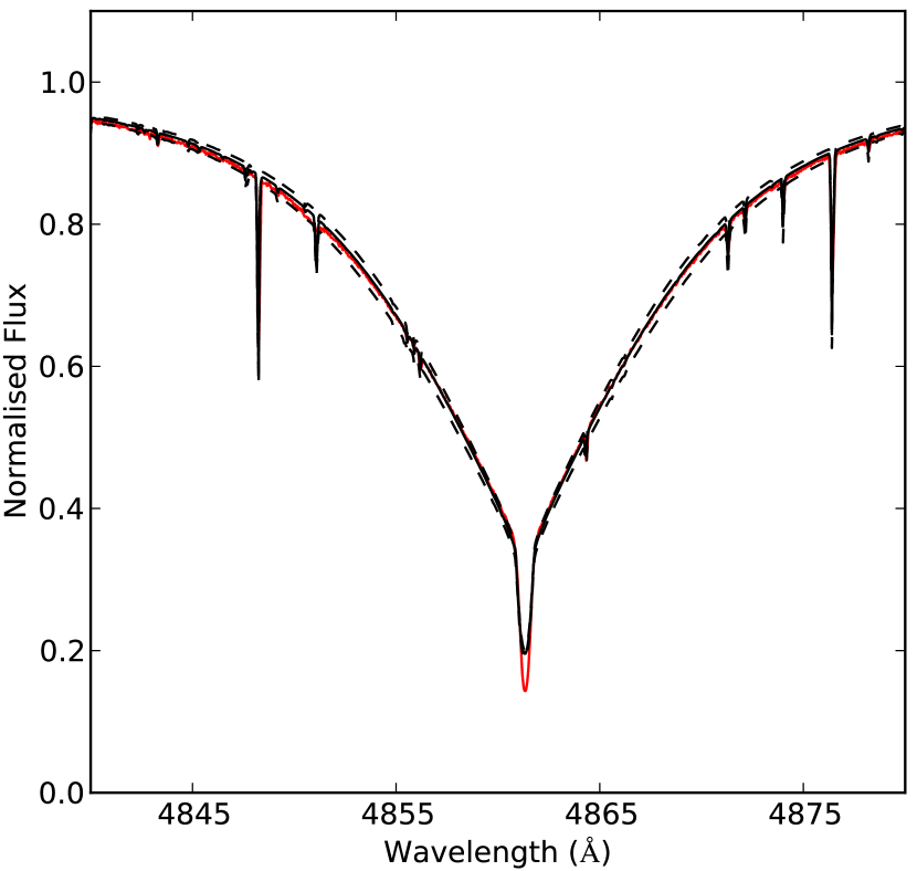
Figure 1: The fit of the H $\beta$ line in the spectrum of 21 Peg. The solid red line is the observed spectrum. The dashed black is the synthetic spectrum calculated using $T_{\rm eff}=10400$ K and $\log g=3.55$. The two dashed blue lines are $\pm$ 200K

Table 1: The fundamental parameters associated with the Sun. Calculated both by Prsa et al. (2016) and by the method used in this work.

Fundamental parameters	Prsa et al. (2016)	This work
$T_{\rm eff}$ (K)	5777	5800 $\pm$	200
$\log g$ (cgs)	4.438	4.49 $\pm$	0.1
$v\sin i$ (km s-1)	1.2	2.6 $\pm$	0.1
$v_{\rm mic}$ (km s-1)	0.875	1.0 $\pm$	0.03

Table 2: The fundamental parameters associated with HD32115. Calculated both by Fossati et al. (2011b) and by the method used in this work.

Fundamental parameters	Fossati et al. (2011b)		This work
$T_{\rm eff}$ (K)	7250 $\pm$	100	7300 $\pm$	200
$\log g$ (cgs)	4.2 $\pm$	0.1	4.2 $\pm$	0.1
$v\sin i$ (km s-1)	8.3 $\pm$	0.5	14.21 $\pm$	0.07
$v_{\rm mic}$ (km s-1)	2.5 $\pm$	0.2	2.5 $\pm$	0.02

Table 3: The fundamental parameters associated with the 21 Peg. Calculated both by Fossati et al. (2009) and by the method used in this work.

Fundamental Parameters	Fossati et al. (2009)		This work
$T_{\rm eff}$ (K)	10400 $\pm$	200	10400 $\pm$	200
$\log g$ (cgs)	3.55 $\pm$	0.1	3.5 $\pm$	0.1
$v\sin i$ (km s-1)	3.76 $\pm$	0.35	4.2 $\pm$	0.1
$v_{\rm rad}$ (km s-1)	0.5 $\pm$	0.5	0.40 $\pm$	0.04
$v_{\rm mic}$ (km s-1)	0.5 $\pm$	0.5	0.4 $\pm$	0.2

Table 4: A comparison between the chemical abundances of the Sun calculated by Asplund et al. (2009) and those calculated by sparti_simple.

	$\log\left(N/{\rm H}\right)$
	Asplund et al.		Sparti
Element	(2009)		Simple		$\Delta$
Mg	7.60 $\pm$	0.04	7.63 $\pm$	0.02	-0.03
Ti	4.95 $\pm$	0.05	4.96 $\pm$	0.01	-0.01
V	3.93 $\pm$	0.08	3.97 $\pm$	0.01	-0.04
Cr	5.64 $\pm$	0.04	5.60 $\pm$	0.01	0.04
Fe	7.50 $\pm$	0.04	7.49 $\pm$	0.01	0.01
Ni	6.22 $\pm$	0.04	6.21 $\pm$	0.01	0.01

Table 5: A comparison between the chemical abundances of 21 Peg calculated by Fossati et al. (2009) and those calculated by sparti_simple, along with the solar abundances from Asplund et al. (2009).

	$\log\left(N/{\rm H}\right)$
	Fossati et al.		sparti
Element	(2009)		simple		$\Delta$	Solar
O i	8.76 $\pm$	0.11	8.80 $\pm$	0.06	-0.04	8.69
Al ii	6.34 $\pm$	0.10	6.37 $\pm$	0.16	-0.03	6.45
Si ii	7.55 $\pm$	0.13	7.51 $\pm$	0.07	0.04	7.51
S ii	7.18 $\pm$	0.13	7.24 $\pm$	0.34	-0.06	7.12
Sc ii	2.67 $\pm$	0.10	2.59 $\pm$	0.23	0.08	3.15
Ti ii	4.81 $\pm$	0.09	4.78 $\pm$	0.03	0.03	4.95
V ii	4.06 $\pm$	0.06	3.96 $\pm$	0.05	0.10	3.93
Cr ii	5.84 $\pm$	0.10	5.79 $\pm$	0.02	0.05	5.64
Fe ii	7.54 $\pm$	0.12	7.52 $\pm$	0.01	0.02	7.50
Ni ii	6.43 $\pm$	0.09	6.38 $\pm$	0.03	0.05	6.22
Sr ii	2.94 $\pm$	-	2.91 $\pm$	0.04	0.03	2.87
Ba ii	2.85 $\pm$	0.06	2.81 $\pm$	0.24	0.04	2.18

Table 6: Instrument settings information with the useful spectral lines given for stellar $T_{\rm eff}$ between $\sim 6000$ Å and $\sim 25000\,$Å

Instrument	Resolving	Spectral	Important
setting	power	region ($\AA$)	spectral lines
LR3	7500	4500–5077	H$\,\beta$
HR9B	25900	5139–5355	Fe-peak (inc. Fe,Ti and Cr)
			Mg triplet at $\lambda$’s
			$\sim$ 5167, 5172 and 5183 $\AA$
HR11	24200	5592–5838	Fe, Na and Sc
LR6	8600	6438–6822	H $\alpha$
UVES	47000	4140–6210	H $\beta$, H $\gamma$
			Fe-peak (inc. Fe,Ti and Cr)
			Mg triplet at $\lambda$’s
			$\sim$ 5167, 5172 and 5183 Å

Table 7: List of programme stars. The proper motion ($\mu$) in right ascension (RA) and declination (DEC), for each star, is taken from the UCAC2 catalogue (Zacharias et al., 2005). The radial velocities ($v_{\rm r}$) are calculated using the method in Section 6.1 and for the member stars using sparti_simple. $\Delta$ is the number of standard deviations the proper motions and radial velocity are away from the cluster mean. The S/N (column 8) corresponds to the S/N per spectral bin of either the GIRAFFE settings or the UVES 520 nm setting. The $BV$ photometry is taken from the APASS catalogue (Henden et al., 2016) and the $JK$ photometry is taken from the UCAC2 catalogue (Zacharias et al., 2005). The Memb. column gives the results of our membership analysis, where ‘y’ means the star is a member, ‘n’ means the star is not a member. The final column gives the membership probabilities given by Dias et al. (2006).

Star	$\mu_{\rm RA}$		$\Delta_{\mu_{\rm RA}}$	$\mu_{\rm DEC}$		$\Delta_{\mu_{\rm DEC}}$	$v_{\rm r}$		$\Delta_{v_{\rm r}}$	S/N	Phot. (Mag)					Dias
name	$(\rm masyr^{-1})$			$(\rm masyr^{-1})$			$(\rm kms^{-1})$			LR3/HR9B/HR11/LR6	$B$	$V$	$J$	$K$	Memb.	Memb.
CD-4511088	2.4$\pm$	1.4	0.6	$-$3.5$\pm$	1.4	0.4	$-$36.0$\pm$	0.5	2.6	94/95/128/122	11.4	11.0	10.4	10.1	n
HD 152706	$-$2.9$\pm$	1.4	1.0	$-$3.3$\pm$	1.3	0.5	$-$4.6$\pm$	0.4	0.5	68[UVES]	10.4	10.1	9.7	9.5	y
HD 152743	0.3$\pm$	1.4	0.0	$-$4.6$\pm$	1.4	0.1	0.4$\pm$	52.4	1.0	116/252/146/194	9.2	9.1	8.7	8.6	y
HD 329261	$-$10.0$\pm$	0.5	3.3	$-$19.0$\pm$	0.5	4.7	$-$3.1$\pm$	0.5	0.7	59/62/84/128	11.2	10.8	9.9	9.6	n
HD 329268	$-$6.0$\pm$	0.5	2.0	$-$7.0$\pm$	0.5	0.7	$-$20$\pm$	3.0	1.0	62/69/92/72	12.0	11.4	10.6	10.3	n
HD 329269	4.0$\pm$	0.5	1.1	$-$13.0$\pm$	0.5	2.7	$-$16$\pm$	3.0	0.6	58/60/84/118	11.7	11.2	9.9	9.6	n
NGC 6250-11	17.5$\pm$	1.4	5.3	$-$23.6$\pm$	1.4	6.3	1$\pm$	3.0	1.1	51/62/75/72	13.4	12.7	11.4	11.0	n
NGC 6250-13	2.7$\pm$	2.5	0.7	$-$3.1$\pm$	2.4	0.6	$-$14$\pm$	3.0	0.4	49/59/70/58	13.5	13.1	12.0	11.6	y
TYC 8327-565-1	$-$0.5$\pm$	1.7	0.3	$-$1.6$\pm$	1.7	1.1	$-$9.4$\pm$	0.2	0.1	65[UVES]	11.0	10.8	10.5	10.4	y
UCAC 12065030	$-$2.4$\pm$	5.2	0.9	$-$17.9$\pm$	5.2	4.4	$-$20$\pm$	3.0	1.0	43/53/62/49	14.2	13.5	11.8	11.4	n	47
UCAC 12065057	$-$14.4$\pm$	2.6	4.6	$-$21.2$\pm$	2.4	5.5	$-$49$\pm$	3.0	3.9	50/59/72/61	13.6	12.9	11.4	10.9	n	100
UCAC 12065058	11.9$\pm$	5.2	3.6	$-$14.7$\pm$	5.2	3.3	85.0$\pm$	0.2	9.5	40/43/53/48	14.9	14.1	12.6	12.1	y*	79
UCAC 12065064	1.3$\pm$	2.6	0.3	$-$4.2$\pm$	2.4	0.2	$-$14.5$\pm$	0.6	0.5	45/54/62/54	14.0	13.5	12.4	12.1	y	3
UCAC 12065075	$-$0.8$\pm$	2.6	0.4	1.5$\pm$	2.4	2.1	18.4$\pm$	0.1	2.8	45/52/63/58	14.1	13.4	12.1	11.8	y*	10
UCAC 12284480	1.5$\pm$	5.2	0.3	$-$10.9$\pm$	5.2	2.0	17$\pm$	3.0	2.7	38/39/46/47			12.7	11.9	n	14
UCAC 12284506	$-$4.5$\pm$	2.6	1.5	$-$11.3$\pm$	2.4	2.2	$-$10$\pm$	3.0	0.0	43/54/66/62	13.9	13.2	11.8	11.5	y	16
UCAC 12284534	$-$2.4$\pm$	5.2	0.9	$-$18.8$\pm$	5.2	4.7	$-$70$\pm$	3.0	6.0	38/42/55/51	14.8	13.9	12.1	11.6	n	55
UCAC 12284536	1.0$\pm$	2.5	0.2	$-$3.9$\pm$	2.4	0.3	$-$12.5$\pm$	6.7	0.2	63/77/93/74	12.8	12.4	11.5	11.4	y	3
UCAC 12284546	1.9$\pm$	5.7	0.5	$-$3.4$\pm$	1.8	0.5	$-$16.1$\pm$	2.3	0.6	52/63/75/55	13.3	12.9	11.9	11.6	y	4
UCAC 12284585	$-$6.2$\pm$	1.4	2.1	$-$8.9$\pm$	1.4	1.4	51$\pm$	3.0	6.1	48/54/65/62	13.2	12.5	11.1	10.6	n	20
UCAC 12284589	$-$5.1$\pm$	3.0	1.7	$-$5.5$\pm$	1.8	0.2	$-$12$\pm$	3.0	0.2	76/101/104/103	12.1	11.8	11.2	11.0	y	7
UCAC 12284594	0.8$\pm$	5.2	0.1	$-$3.1$\pm$	5.2	0.6	9.7$\pm$	0.3	2.0	40/42/56/48	14.6	13.9	12.5	12.1	y	7
UCAC 12284608	3.5$\pm$	5.2	1.0	$-$31.0$\pm$	5.2	8.7	$-$55$\pm$	3.0	4.5	36/38/44/49	15.3	14.3	12.3	11.6	n	100
UCAC 12284620	$-$6.3$\pm$	5.2	2.1	$-$27.1$\pm$	5.2	7.4	$-$55$\pm$	3.0	4.5	41/46/56/55	14.3	13.4	11.8	11.3	n	98
UCAC 12284626	$-$11.5$\pm$	5.2	3.7	$-$28.6$\pm$	5.2	7.9	$-$15$\pm$	3.0	0.5	40/45/49/56	14.3	13.5	12.1	11.7	n	100
UCAC 12284628	2.9$\pm$	1.4	0.8	$-$10.5$\pm$	3.4	1.9	$-$45.0$\pm$	0.5	3.5	53/72/80/66	13.0	12.7	11.8	11.6	y*	14
UCAC 12284631	2.9$\pm$	1.4	0.8	$-$5.1$\pm$	1.4	0.1	$-$0.9$\pm$	0.2	0.9	62/81/97/79	11.8	11.3	11.3	11.0	y	4
UCAC 12284638	1.0$\pm$	1.5	0.2	$-$1.4$\pm$	1.5	1.1	$-$6$\pm$	3.0	0.4	57/72/89/69	12.0	11.8	11.7	11.4	y	3
UCAC 12284645	0.4$\pm$	1.4	0.0	$-$2.3$\pm$	1.4	0.8	$-$19.0$\pm$	9.2	0.9	65/76/96/72	12.8	12.4	11.5	11.2	y	2
UCAC 12284653	3.3$\pm$	5.4	0.9	$-$3.3$\pm$	5.2	0.5	$-$13.4$\pm$	0.6	0.3	36/36/38/42			13.1	12.6	y	8
UCAC 12284662	3.5$\pm$	5.3	1.0	$-$10.6$\pm$	5.2	1.9	$-$14.9$\pm$	0.9	0.5	44/46/56/53	14.4	13.8	12.3	11.9	y	16
UCAC 12284746	0.1$\pm$	5.2	0.1	$-$4.3$\pm$	5.4	0.2	$-$10.9$\pm$	0.2	0.1	36/39/46/48			12.5	12.2	y	7
** Star considered as members based only on photometry.

4 Observations of NGC 6250

4.1 Target

The cluster NGC 6250 is located in the constellation Ara in the Southern hemisphere. Using proper motions and photometry from PPMXL (Roeser et al., 2010) and 2MASS (Skrutskie et al., 2006) $JHK$ photometry data, Kharchenko et al. (2013) have estimated the age of the cluster to be $\log t\sim 7.42$ yr and the distance from the Sun to the cluster as 865 pc. Kharchenko et al. (2013) calculated the cluster proper motion as $0.7\,\pm\,0.4$ mas yr^-1 in right ascension (RA) and $-4.1\,\pm\,0.4$ mas yr^-1 in declination (DEC) with a cluster radial velocity of $-8.0\,\pm\,0.8$ km s^-1. Previously, Herbst (1977) estimated $\log t\sim 7.146$ yr for the age and 1025 pc for the distance. Moffat & Vogt (1975) estimated $d=950$ pc. NGC 6250 is located in a dust-rich region of space, with $E$ ($B$ – $V$) = 0.385 and $E$ ($J$ – $H$) = 0.123 (Kharchenko et al., 2013). To our best knowledge, the cluster has not previously been studied in detail spectroscopically, except for the purpose of classification spectra and radial velocity measurements.

4.2 Instrument

The observations of NGC 6250 were obtained in service mode on 2007 May 27 and 30 using FLAMES, the multi-object spectrograph attached to the Unit 2 Kueyen of the ESO/VLT.

The FLAMES instrument (Pasquini & et al., 2002) is able to access targets over a field of view of 25 arcmin in diameter. Its 138 fibres feed two spectrographs, GIRAFFE and the Ultraviolet and Visual Echelle Spectrograph (UVES). This makes it possible to observe up to 138 stars, 130 using GIRAFFE linked to FLAMES with MEDUSA fibres, and 8 using UVES linked to FLAMES with UVES fibres. FLAMES-GIRAFFE can obtain low- or medium-resolution spectra ($R$ = 7500–30 000), within the spectral range 3700–9000 Å. Low-resolution spectra may be obtained within wavelength intervals 500–1200 Å wide; medium-resolution spectra are obtained in wavelength intervals 170–500 Å wide. FLAMES-UVES can obtain high-resolution spectra ($R$ = 47 000), with central wavelengths of 5200, 5800 or 8600 Å  each covering a wavelength range $\sim 2000$ Å wide.

4.3 Instrument Settings

For the observations, we chose the instrument set-up that allowed us: (1) to observe two hydrogen lines, which are essential to the determination of $T_{\rm eff}$ and $\log$ $g$ and (2) to maximize the number of metal lines and consequently the number of chemical elements available for spectral analysis. The GIRAFFE settings were chosen such that they are as close to the guiding wavelength of 520 nm as possible, in an effort to minimize light losses due to atmosphere differential refraction. The higher spectral resolution of UVES means that, to achieve a high enough S/N ratio for each spectra, UVES requires an exposure time typically three or four times that of GIRAFFE. As a result during UVES observations we are able to obtain observations with three GIRAFFE settings. The settings we used are shown in Table 6. We observed with the HR9B and HR11 settings both observing nights and one L- setting each night.

To prevent saturation of the observations each UVES observation was divided into four sub-exposures and each GIRAFFE setting was divided into two sub-exposures.

4.4 Data reduction

Our data were obtained in service mode, and the package released included the products reduced by ESO with the instrument dedicated pipelines. In this work, we used the low- and mid resolution GIRAFFE data as reduced by ESO and re-reduced UVES spectra.

For the normalization we followed a standard procedure. First, we fit the observed spectrum with a function $G(\lambda)$, clipping in an iterative way all points 3 $\sigma$ above and 1 $\sigma$ below the spectrum. Then, we compare the normalized spectrum with a synthetic spectrum calculated adopting a similar stellar model, in order to test the quality of our normalization. Experience has shown for the low-resolution settings LR3 and LR6, a third-order polynomial gives the best normalization. For UVES and the high-resolution settings HR9B and HR11, a cubic spline gives the best normalization. In the case of UVES the Balmer lines spread across two different orders, the merging of the orders was therefore done before the normalization.

5 Cluster membership

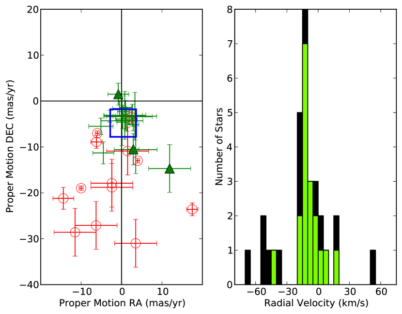
Figure 2: Left-hand panel: the proper motion of the observed stars from the UCAC2 catalogue (Zacharias et al., 2005). Green plus-signs are stars we consider to be members and red circles are stars we do not consider to be members. Triangles are the stars for which membership is considered based solely on photometry. The remaining points are stars for which membership is considered based on the kinematics and photometry. The blue box is centred at the cluster mean proper motions and represents the uncertainty of these values in each direction. Right-hand panel: histogram of the radial velocity measurements calculated using the method described in Section 6.1 for non-member stars and for the member stars using sparti_simple. The green histogram highlights the radial velocity of the cluster members.

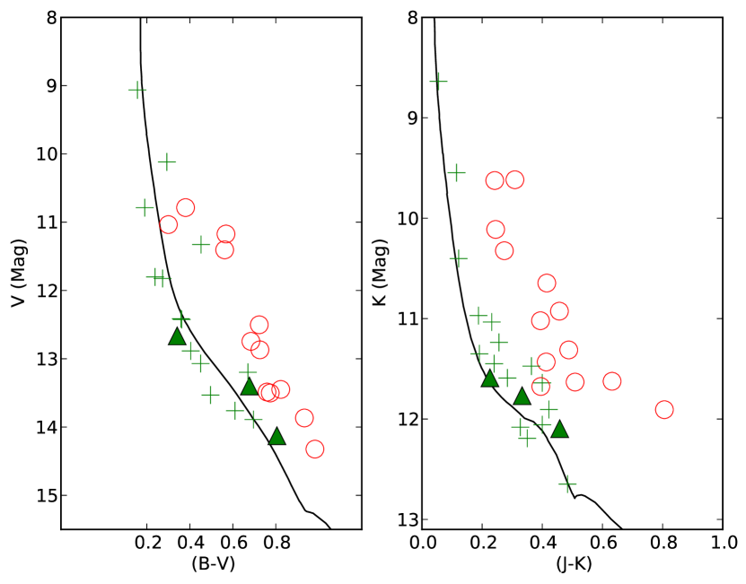
Figure 3: In both panels, green plus-signs are stars we consider members and red circles are stars we do not consider to be members. Triangles are the stars for which membership is considered based solely on photometry. The remaining points are stars for which membership is considered based on the kinematics and photometry. Left-hand panel: optical colour–magnitude diagram of the observed stars. The $BV$ photometry is taken from the APASS catalogue (Henden et al., 2016), plotted with the isochrone at ($\log t\sim 7.42$) corrected for $E$ ($B$ – $V$) = 0.385 (Kharchenko et al., 2013, black solid line). Right-hand panel: infrared colour–magnitude diagram of the observed stars. The $JK$ photometry is taken from the UCAC2 catalogue (Zacharias et al., 2005), plotted with the isochrone at ($\log t\sim 7.42$) corrected for $E$ ($J$ – $K$) = 0.200 (Kharchenko et al., 2013, black solid line).

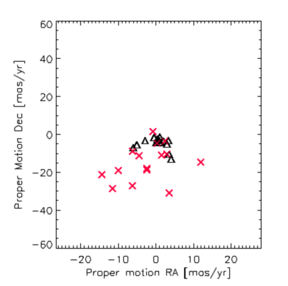
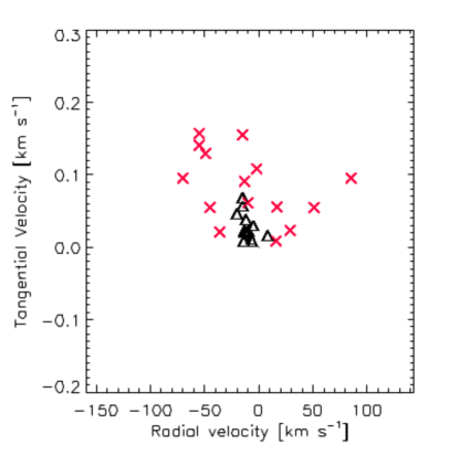
Figure 4: $K$-means clustering result for the membership analysis of NGC6250: the black triangles are member stars and the red crosses are non-members. The left-hand panel shows the sample distribution in proper motion. The right-hand panel shows the sample distribution in velocity. The tangential velocity was computed using the distance 850 pc given by Kharchenko et al. (2013)

Previous studies by Bayer et al. (2000), Dias et al. (2006) and Feinstein et al. (2008) give cluster membership information for the stars in the vicinity of NGC 6250. Dias et al. (2006) estimate cluster membership using the statistical method of Sanders (1971). The probabilities are shown in Table 7. Note that some of the results of Dias et al. (2006) show inconsistencies: three stars (UCAC 12065057, UCAC 12284608 and UCAC 12284626) have been assigned 100 % likelihood of being members despite their proper motion values being far from the cluster mean (which they calculate to be consistent with Kharchenko et al., 2013). Furthermore, UCAC 12065064 has proper motion values very close to the cluster mean values and its photometry fits well with the theoretical isochrone, it only has a 3 % likelihood of being a member.

The determination of cluster membership from previous literature was used as a guess for an initial target selection. Our new spectroscopic data allow a refined membership study, which is critical for our analysis.

5.1 Proper motion and radial velocity membership

The proper motions and radial velocities of the observed stars are shown in Table 7 and are plotted in Fig. 2. In our membership analysis we have followed two methods.

First, we have identified those stars that are within 1 $\sigma$ of the mean proper motion and radial velocity values for our sample. This way we have identified 19 stars to be members of the cluster. We calculate the cluster mean proper motions as, 0.1 $\pm$ 2.9 mas yr^-1 in RA, $-$6.1 $\pm$ 4.4 mas yr^-1 in DEC and radial velocity of $-$10 $\pm$ 11 km s^-1.

As a cross-check, we also use the partitional clustering technique, $K$-means clustering (MacQueen, 1967). It is a technique to find common data points based on the analysis of the variables that define the data. In general, the method is to set a predicted number of data clusters and give an initial guess for the centres of these clusters. The algorithm then assigns points to the closest cluster centre and recalculates until the cluster centre values do not change. Our problem is simplified by the fact that we can define one cluster centre close to the literature value of cluster proper motion and radial velocity. In practice, we have set the number of clusters to 5: one initially centred in the literature values $(\mu_{0},v_{r_{0}})$ and the other four initially centred respectively at $(\mu_{0}+1.5\,\sigma_{\mu},v_{r_{0}})$, $(\mu_{0}-1.5\,\sigma_{\mu},v_{r_{0}})$, $(\mu_{0},v_{r_{0}}+1.5\,\sigma_{v_{r}})$ and $(\mu_{0},v_{r_{0}}+1.5\,\sigma_{v_{r}})$, where $\sigma_{v_{r}}$ and $\sigma_{\mu}$ are the standard deviation in our sample. We have performed this computation using the CLUSTER function in idl.

Fig. 4 shows the results of our cluster analysis. We found 15 members and we calculated the cluster mean proper motions as 0.4 $\pm$ 3.0 mas yr^-1 in RA, $-$4.80 $\pm$ 3.2 mas yr^-1 in DEC and radial velocity of $-$10 $\pm$ 6 km s^-1. Both methods give the same results apart from four stars. The discrepancy between the two methods is likely because the spread of radial velocity is large and asymmetric, and the $K$-means clustering is able to deal with this more effectively.

5.2 Photometry

The magnitude and colour of our sample of stars are a good indicator of cluster membership. Using the $B$ and $V$ magnitudes from Henden et al. (2016) and the $J$ and $K$ magnitudes from Zacharias et al. (2005), we have produced two colour magnitude diagrams, displayed in Fig. 3. Each diagram shows the photometry and a theoretical isochrone calculated with CMD 2.7 (Bressan et al., 2012; Chen et al., 2014; Tang et al., 2014; Chen et al., 2015) for an age of $\log t=7.42$. The photometry has been corrected for the extinction (Kharchenko et al., 2013) and distance to the cluster (850 pc; Kharchenko et al., 2013).

In general, we see very good agreement between the member stars determined using the kinematics approach and those that fit the isochrones. Notable exceptions are UCAC 12065058, UCAC 12065075 and UCAC 12284628, which do not agree with the kinematics of the cluster mean, but agree very well with the photometry. This maybe as a result of a re-ejection event and so we consider these stars as members.

6 Fundamental parameters

6.1 Radial velocity and rotational velocity

We have calculated initial values of $v_{\rm rad}$ and $v\sin i$ from the FLAMES spectra obtained in the range 5150–5350 Å with the highest resolution setting HR9B. We used a least-squares deconvolution (LSD; Kochukhov et al., 2010) of the observed spectrum with lines selected from the VALD list (Piskunov et al., 1995) to calculate an average line profile in velocity space. To do the line selection, we must have an estimate of the temperature, so we use a combination of Balmer lines and photometry to determine an estimate of the temperature.

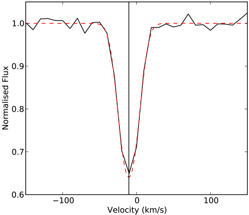
Figure 5: The least-square deconvolution of the spectrum of UCAC 12284746 ($T_{\rm eff}=7200$ K) (solid black line), plotted against the Gaussian fit (red dashed line). The radial velocity is given by the position of the centre of the Gaussian, and it is indicated by a solid vertical line.

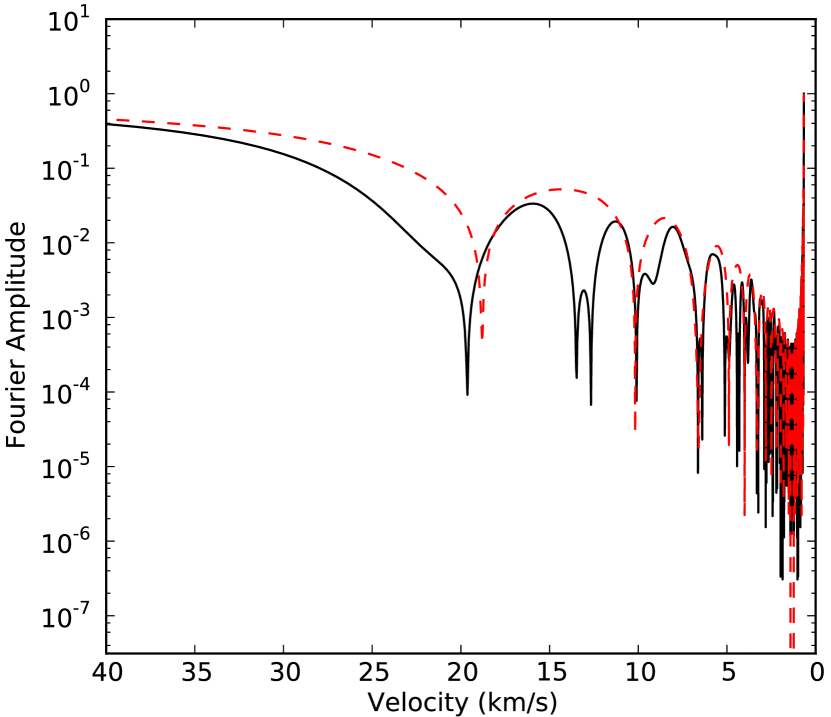
Figure 6: The fast Fourier transform of the LSD profile of Fig. 5 (black solid line), plotted with the FTT of a model LSD profile with $T_{\rm eff}=7200$ K and $v\sin i=19.5$  km s^-1 (red dashed lines).

The radial velocity of each star has been estimated using a Gaussian fit, as shown in Fig. 5.

In order to measure $v\sin i$  the LSD profile is then shifted to the rest frame, and the fast Fourier transform (FFT) is calculated. An example of the FFT is shown in Fig. 6. Following Gray (2005), the first minimum of the FFT corresponds to the stellar $v\sin i$ value. Glazunova et al. (2008) showed that it is possible to use the LSD profile, in place of the more noisy profiles of single lines, to derive the $v\sin i$ value using the FFT method described by Gray (2005). Because we expect low $v_{\rm mac}$ values (Grassitelli et al., 2015), at the resolution of FLAMES $v_{\rm mac}$ cannot be distinguished from $v\sin i$ and we therefore ignore it.

6.2 Fundamental parameters from Balmer lines

We deduced the fundamental parameters $T_{\rm eff}$ and $\log g$ by fitting synthetic and observed Balmer lines H $\beta$ and H $\gamma$ for UVES spectra and H $\alpha$ and H $\beta$ for GIRAFFE spectra. Model atmospheres were computed with atlas9 (Kurucz, 1993b) assuming plane parallel geometry, local thermodynamical equilibrium and opacity distribution function (ODF) for solar abundances (Kurucz, 1993a). The synthetic spectra were computed with cossam_simple. Examples of the fit between our model and the observed Balmer lines are shown in Fig. 9.

We used hydrogen line as both temperature and gravity indicator because for $T_{\rm eff}\la 8000$ K they are more sensitive to temperature and for higher temperature they are more sensitive to $\log g$ variation but temperature effects can still be visible in the part of the wing close to the line core, according to Fossati et al. (2011a).

To check our values of $\log g$ for each star we determined the $\log g$ which provided the best ionization balance between Fe i and Fe ii lines. To test this method, we calculate the abundance of Fe i and Fe ii for the Sun using $T_{\rm eff}$ = 5800 K and varying the $\log g$ between 3.8 and 4.5. The value of $\log g$ where the abundances of Fe i and Fe ii are equal is 4.49 compared with 4.44 found by (Prsa et al., 2016). We performed a similar analysis for 21 Peg, varying the $\log g$ between 3.5 and 4.2 and using $T_{\rm eff}$ = 10400 K. As a result we calculate a value for $\log g$ of 3.5 compared with 3.55 found by Fossati et al. (2009). The results of this analysis are shown in Figs 7 and Figs 8. For each of the NGC 6250 stars, the $\log g$ values found using both methods agree within the uncertainties.

As a result of the low S/N, we were unable to measure any abundances for TYC 8327-565-1 and UCAC 12284638; however, we were able to estimate $T_{\rm eff}$ and $\log g$ that are given in Table 8.

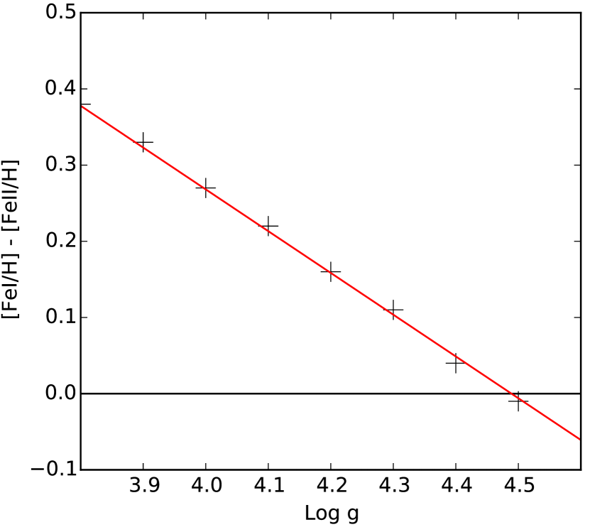
Figure 7: The difference between the abundance of Fe i and Fe ii plotted as a function of surface gravity for the Sun determined using sparti_simple by varying the $\log g$ of the model atmosphere at $T_{\rm eff}$ = 5800K.

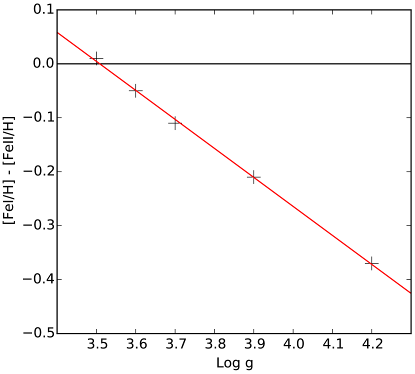
Figure 8: The difference between the abundance of Fe i and Fe ii plotted as a function of surface gravity for the star 21Peg determined using sparti_simple by varying the $\log g$ of the model atmosphere at $T_{\rm eff}$ = 10400K.

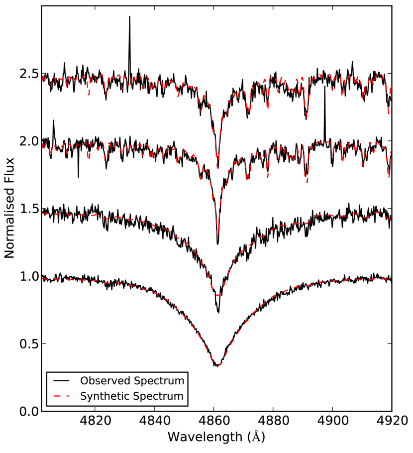
Figure 9: A sample of the observed H $\beta$ lines (black solid lines) fitted with the model spectra (red dashed line). From top to bottom the stars are: UCAC 12284594 ($T_{\rm eff}=6200$ K), UCAC 12065075 ($T_{\rm eff}=6300$ K), UCAC 12065064 ($T_{\rm eff}=7600$ K) and UCAC 12284536 ($T_{\rm eff}=9800$ K). Each profile is calculated with $v\sin i$ as shown in Table 8.

Table 8: Atmospheric parameters for the sample of stars from NGC 6250.

Star	$T_{\rm eff}$		$\log g$		$v_{\rm mic}$		$v\sin i$
	(K)		(CGS)		( km s-1)		( km s-1)
HD 152706	9900 $\pm$	200	4.2 $\pm$	0.1	1.9 $\pm$	0.1	151.6 $\pm$	0.2
HD 152743	19 800 $\pm$	200	4.1 $\pm$	0.1	2.1 $\pm$	2.5	198.9 $\pm$	12.7
NGC 6250-13	8200 $\pm$	200	4.2 $\pm$	0.1	2.0 $\pm$	0.1	70.1 $\pm$	0.8
TYC 8327-565-1	14 200 $\pm$	500	4.2 $\pm$	0.3	–		–
UCAC 12065058	6000 $\pm$	200	4.4 $\pm$	0.1	0.9 $\pm$	0.2	4.8 $\pm$	0.9
UCAC 12065064	7600 $\pm$	200	4.2 $\pm$	0.1	0.3 $\pm$	0.4	54.1 $\pm$	0.7
UCAC 12065075	6300 $\pm$	200	4.4 $\pm$	0.1	1.0 $\pm$	0.1	15.2 $\pm$	0.2
UCAC 12284506	6100 $\pm$	200	4.4 $\pm$	0.1	0.6 $\pm$	0.1	10.6 $\pm$	0.2
UCAC 12284536	10 000 $\pm$	200	4.4 $\pm$	0.1	2.0 $\pm$	0.2	170.2 $\pm$	3.6
UCAC 12284546	8400 $\pm$	200	4.2 $\pm$	0.1	0.3 $\pm$	0.5	146.0 $\pm$	1.5
UCAC 12284589	12 600 $\pm$	200	4.2 $\pm$	0.1	0.5 $\pm$	0.7	215.5 $\pm$	2.7
UCAC 12284594	6100 $\pm$	200	4.4 $\pm$	0.1	0.3 $\pm$	0.2	50.3 $\pm$	0.5
UCAC 12284628	10 000 $\pm$	200	4.3 $\pm$	0.1	0.3 $\pm$	0.5	22.9 $\pm$	0.8
UCAC 12284631	9800 $\pm$	200	4.2 $\pm$	0.1	0.7 $\pm$	0.2	17.8 $\pm$	0.4
UCAC 12284638	10 800 $\pm$	400	4.2 $\pm$	0.3	–		–
UCAC 12284645	11 000 $\pm$	200	4.3 $\pm$	0.1	2.0 $\pm$	0.4	270.0 $\pm$	3.0
UCAC 12284653	6200 $\pm$	200	4.4 $\pm$	0.1	1.5 $\pm$	0.2	49.5 $\pm$	1.0
UCAC 12284662	7400 $\pm$	200	4.4 $\pm$	0.1	2.0 $\pm$	0.1	81.4 $\pm$	0.9
UCAC 12284746	7200 $\pm$	200	4.3 $\pm$	0.1	1.8 $\pm$	0.2	24.5 $\pm$	0.4

Table 9: The abundance of elements for the analysed stars of NGC6250 (ordered by decreasing $T_{\rm eff}$), given in log($N$/H) where H = 12.00. In parenthesis, the first number is the error calculated using equation (3) and the second in the error calculating using equation (5). Both errors are in units of 0.01dex. The last row of each set gives the solar abundances from Asplund et al. (2009).

Star	$T_{\rm eff}$	$v\sin i$		C	O	Na	Mg	Si	S
	(K)	(km s-1)
HD 152743	19 800	198.9 $\pm$	12.7					8.07 (95;102)
UCAC 12284589	12 600	215.5 $\pm$	2.7
UCAC 12284645	11 000	270.0 $\pm$	3.0
UCAC 12284628	10 000	22.9 $\pm$	0.8				6.41 (06;12)
UCAC 12284536	10 000	170.2 $\pm$	3.5				7.58 (25;27)
HD 152706	9900	151.6 $\pm$	0.2	8.91 (02;34)	8.68 (02;04)		7.99 (02;28)	7.83 (02;27)
UCAC 12284631	9800	17.8 $\pm$	0.4	8.84 (13;16)			6.61 (04;12)	7.98 (11;27)
UCAC 12284546	8400	146.0 $\pm$	1.5	8.83 (09;15)			6.19 (15;67)
NGC 6250-13	8200	70.1 $\pm$	0.8				7.74 (06;14)
UCAC 12065064	7600	54.1 $\pm$	0.7	8.63 (11;15)			7.29 (08;13)	7.39 (08;15)	7.92 (11;59)
UCAC 12284662	7400	81.4 $\pm$	0.9	8.50 (19;37)		6.24 (17;20)	7.59 (09;13)	7.51 (10;10)
UCAC 12284746	7200	24.5 $\pm$	0.4	8.92 (13;14)		6.25 (13;15)	7.68 (10;15)	7.26 (10;11)
UCAC 12065075	6300	15.2 $\pm$	0.2			6.49 (07;22)	7.64 (04;22)	7.34 (04;19)
UCAC 12284653	6200	49.5 $\pm$	1.0			6.37 (21;26)	7.58 (11;19)	7.50 (13;14)
UCAC 12284594	6100	50.3 $\pm$	0.5			6.24 (09;10)	7.45 (03;12)	7.11 (06;07)
UCAC 12284506	6100	10.6 $\pm$	0.2	8.91 (08;26)		6.05 (05;07)	7.28 (01;10)	6.94 (03;04)	7.81 (28;46)
UCAC 12065058	6000	4.8 $\pm$	0.9			6.08 (17;17)	7.70 (08;12)	6.91 (12;12)
Solar	5777	1.2		8.43	8.69	6.24	7.60	7.51	7.12
Star	$T_{\rm eff}$	$v\sin i$		Ca	Sc	Ti	V	Cr	Mn
	(K)	(km s-1)
HD 152743	19 800	198.9 $\pm$	12.7
UCAC 12284589	12 600	215.5 $\pm$	2.7					6.25 (14;18)
UCAC 12284645	11 000	270.0 $\pm$	3.0			4.96 (28;35)		5.64 (23;32)
UCAC 12284628	10 000	22.9 $\pm$	0.8			4.94 (11;16)		5.57 (09;10)
UCAC 12284536	10 000	170.2 $\pm$	3.5			5.02 (23;23)		5.73 (21;23)
HD 152706	9900	151.6 $\pm$	0.2	6.92 (02;46)		4.95 (02;04)		5.78 (02;16)
UCAC 12284631	9800	17.8 $\pm$	0.4			4.75 (06;08)		5.49 (07;08)
UCAC 12284546	8400	146.0 $\pm$	1.5	7.14 (22;22)		5.05 (09;19)		6.14 (07;20)
NGC 6250-13	8200	70.1 $\pm$	0.8	6.22 (08;14)		4.83 (05;08)		5.75 (06;09)	5.51 (13;17)
UCAC 12065064	7600	54.1 $\pm$	0.7	6.63 (17;24)		5.24 (02;08)		5.95 (07;12)	5.63 (23;35)
UCAC 12284662	7400	81.4 $\pm$	0.9	6.32 (12;21)	3.13 (14;23)	4.97 (06;14)		5.69 (08;23)	5.45 (16;21)
UCAC 12284746	7200	24.5 $\pm$	0.4	6.19 (13;16)	3.11 (11;12)	5.23 (06;10)		5.92 (07;10)	5.46 (16;18)
UCAC 12065075	6300	15.2 $\pm$	0.2	6.55 (07;21)	3.41 (05;11)	5.12 (03;13)	4.44 (07;18)	5.92 (03;17)	5.27 (10;15)
UCAC 12284653	6200	49.5 $\pm$	1.0	6.40 (23;28)	2.95 (24;26)	5.19 (09;42)	3.99 (34;55)	6.06 (09;25)	5.62 (23;47)
UCAC 12284594	6100	50.3 $\pm$	0.5	6.33 (09;11)	2.90 (13;14)	5.00 (04;05)	4.78 (07;09)	5.92 (03;08)	5.18 (15;17)
UCAC 12284506	6100	10.6 $\pm$	0.2	6.22 (06;08)	3.16 (05;06)	4.93 (02;05)	3.81 (07;11)	5.53 (02;07)	5.30 (07;09)
UCAC 12065058	6000	4.8 $\pm$	0.9	6.42 (16;16)	3.01 (15;16)	4.92 (08;10)	4.05 (18;20)	5.62 (07;10)	5.25 (22;23)
Solar	5777	1.2		6.34	3.15	4.95	3.93	5.64	5.43
Star	$T_{\rm eff}$	$v\sin i$		Fe	Ni	Zn	Y	Ba	Nd
	(K)	(km s-1)
HD 152743	19 800	198.9 $\pm$	12.7	7.67 (47;49)
UCAC 12284589	12 600	215.5 $\pm$	2.7	7.77 (04;04)
UCAC 12284645	11 000	270.0 $\pm$	3.0	7.50 (12;23)
UCAC 12284628	10 000	22.9 $\pm$	0.8	7.43 (06;10)
UCAC 12284536	10 000	170.2 $\pm$	3.5	7.56 (16;17)
HD 152706	9900	151.6 $\pm$	0.2	7.61 (01;12)
UCAC 12284631	9800	17.8 $\pm$	0.4	7.41 (03;06)
UCAC 12284546	8400	146.0 $\pm$	1.5	7.72 (07;23)	6.94 (10;17)
NGC 6250-13	8200	70.1 $\pm$	0.8	7.54 (04;08)	6.33 (08;13)			2.09 (42;45)
UCAC 12065064	7600	54.1 $\pm$	0.7	7.74 (05;14)	6.16 (11;13)
UCAC 12284662	7400	81.4 $\pm$	0.9	7.51 (07;10)	6.27 (10;28)			2.34 (36;38)
UCAC 12284746	7200	24.5 $\pm$	0.4	7.73 (07;11)	6.30 (08;12)	4.71 (44;46)	2.54 (13;14)	2.18 (49;49)
UCAC 12065075	6300	15.2 $\pm$	0.2	7.65 (03;19)	6.28 (04;14)	4.06 (33;34)	2.38 (11;14)	2.18 (17;17)	1.76 (09;12)
UCAC 12284653	6200	49.5 $\pm$	1.0	7.70 (09;20)	6.44 (11;27)	4.62 (88;88)		2.20 (41;43)
UCAC 12284594	6100	50.3 $\pm$	0.5	7.54 (02;09)	6.15 (06;07)			2.41 (13;14)	1.98 (14;17)
UCAC 12284506	6100	10.6 $\pm$	0.2	7.28 (01;07)	5.99 (03;05)	4.69 (28;28)	2.07 (09;11)	2.42 (09;09)	1.61 (07;13)
UCAC 12065058	6000	4.8 $\pm$	0.9	7.39 (06;09)	6.02 (10;11)			2.18 (39;41)	1.63 (25;25)
Solar	5777	1.2		7.50	6.22	4.56	2.21	2.18	1.42

7 Results and Discussion

The results of the abundance analysis are given in Table 9. Since this is a young cluster, there is the potential for some of the stars to still have discs. If discs were present, we would expect to see the presence of emission lines, particularly in the core of H $\alpha$ and H $\beta$. We do not see any evidence of emission lines in any of the stars.

7.1 UCAC 12284546

UCAC 12284546 shows an overabundance of C, Ca, Cr, Fe and Ni and an underabundance of Mg. However, this abundance pattern does not match any standard chemically peculiar star in this temperature range. To better understand this star, it would be necessary to collect and analyse a higher resolution spectrum with higher S/N. As a result of the abundance anomalies we observe in this star, we do not consider this star in the global analysis of the results.

7.2 Stellar Metallicity

For the evolutionary tracks and isochrones we adopted the metallicity calculated as

$$Z_{\rm cluster}=10^{[{\rm Fe/H}]_{\rm stars}-[{\rm Fe/H}]_{\rm\odot}}Z_{\rm\odot},$$ (6)

where $Z_{\rm cluster}$ and $[{\rm Fe/H}]_{\rm stars}$ are respectively the clusters metallicity and average Fe abundance. This formulation does not follow the definition of $Z$, which is

$$Z=\sum_{i=1}^{n}m_{i}X_{i},$$ (7)

where $n$ is the number of elements, $m_{i}$ is the atomic mass of each element and $X_{i}$ the abundance of each element. In equation (7), $Z$ is driven mostly by the abundance of C and O, which are the most abundant elements following H and He, but in stellar evolutionary calculations the relevant factor is the Fe opacity. This is why for the cluster metallicity we adopt the expression given by equation (6). When using equation (6) to infer the metallicity, it is important to use as Z_⊙ the value adopted by the considered stellar evolution tracks. In this work we use the stellar evolutionary tracks by Bressan et al. (2012), which adopt Z${}_{\rm\odot}=0.0152$. Using the average Fe abundance obtained from the non-chemically peculiar stars, we obtain $Z_{\rm cluster}=0.018\pm 0.005$, which is consistent with the solar value within the uncertainty.

7.3 Spectroscopic H-R diagram

We plot a spectroscopic H-R diagram (Fig. 10) using the $T_{\rm eff}$ and $\log g$ values calculated for each star. We calculate the flux weighted luminosity, $\log\mathcal{L}/\mathcal{L}_{\odot}$, following Langer & Kudritzki (2014) with

$$\log\mathcal{L}/\mathcal{L}{\rm\odot}=\log\left(\frac{T_{\rm eff}^{4}}{g}\right)-\log\left(\frac{T_{\rm eff\odot}^{4}}{g_{\odot}}\right)$$ (8)

where $T_{\rm eff}$ and $\log g$ are taken from Table 8, $T_{\rm eff\odot}$ is the solar effective temperature and $g_{\odot}$ is the solar surface gravity. The isochrones are from Bressan et al. (2012). Based on the H-R diagram, we are not able to constrain the age of this cluster; however, the age of $\log t$ = 7.42 given by Kharchenko et al. (2013) fits well our data. As a result, we use this age in the remainder of the paper. We also give the flux-weighted luminosity, masses and fractional age of each of the stars in Table 10 calculated by fitting evolutionary tracks (Bressan et al., 2012) to each star.

Table 10: $\log\mathcal{L}/\mathcal{L}_{\odot}$, $\log T_{\rm eff}$, $M/M_{\odot}$ and fractional age ($\tau$) with associated error bars for the stars of the NGC 6250 open cluster.

Star	$\log\mathcal{L}/\mathcal{L}_{\odot}$		$\log T_{\rm eff}$		$M/M_{\odot}$		$\tau$
HD 152706	1.17 $\pm$	0.10	4.00 $\pm$	0.02	2.25 $\pm$	1.00	0.02 $\pm$	0.04
HD 152743	2.47 $\pm$	0.06	4.30 $\pm$	0.01	6.40 $\pm$	0.60	0.44 $\pm$	0.09
NGC 6250-13	0.84 $\pm$	0.12	3.91 $\pm$	0.02	1.75 $\pm$	1.00	0.01 $\pm$	0.03
TYC 8327-565-1	1.79 $\pm$	0.21	4.15 $\pm$	0.04	3.80 $\pm$	0.20	0.12 $\pm$	0.14
UCAC 12065058	0.10 $\pm$	0.16	3.78 $\pm$	0.03	1.05 $\pm$	0.10	-0.02 $\pm$	0.01
UCAC 12065064	0.71 $\pm$	0.13	3.88 $\pm$	0.03	1.60 $\pm$	0.05	0.00 $\pm$	0.02
UCAC 12065075	0.18 $\pm$	0.15	3.80 $\pm$	0.03	1.15 $\pm$	0.05	-0.01 $\pm$	0.02
UCAC 12284506	0.13 $\pm$	0.15	3.79 $\pm$	0.03	1.05 $\pm$	0.10	-0.02 $\pm$	0.01
UCAC 12284536	0.98 $\pm$	0.10	4.00 $\pm$	0.02	2.05 $\pm$	0.10	0.02 $\pm$	0.04
UCAC 12284546	0.88 $\pm$	0.12	3.92 $\pm$	0.02	1.80 $\pm$	1.00	0.01 $\pm$	0.03
UCAC 12284589	1.59 $\pm$	0.09	4.10 $\pm$	0.02	3.20 $\pm$	1.00	0.07 $\pm$	0.01
UCAC 12284594	0.13 $\pm$	0.15	3.79 $\pm$	0.03	1.05 $\pm$	0.10	-0.02 $\pm$	0.01
UCAC 12284628	1.08 $\pm$	0.10	4.00 $\pm$	0.02	2.20 $\pm$	0.10	0.02 $\pm$	0.04
UCAC 12284631	1.15 $\pm$	0.11	3.99 $\pm$	0.02	2.20 $\pm$	1.00	0.02 $\pm$	0.04
UCAC 12284638	1.32 $\pm$	0.22	4.03 $\pm$	0.04	2.60 $\pm$	0.20	0.04 $\pm$	0.06
UCAC 12284645	1.25 $\pm$	0.10	4.04 $\pm$	0.02	2.40 $\pm$	0.20	0.03 $\pm$	0.05
UCAC 12284653	0.15 $\pm$	0.15	3.79 $\pm$	0.03	1.10 $\pm$	0.05	-0.02 $\pm$	0.01
UCAC 12284662	0.46 $\pm$	0.13	3.87 $\pm$	0.03	1.40 $\pm$	0.10	-0.00 $\pm$	0.02
UCAC 12284746	0.51 $\pm$	0.13	3.86 $\pm$	0.03	1.45 $\pm$	0.05	-0.00 $\pm$	0.02

Figure 10: An H-R diagram of NGC6250, the stars plotted (black plus-signs) with theoretical isochrones (Bressan et al., 2012) at $\log t$ = 7.40 (dashed black line) and $\log t$ = 7.45 (solid black line). Both isochrones have solar metallicity.

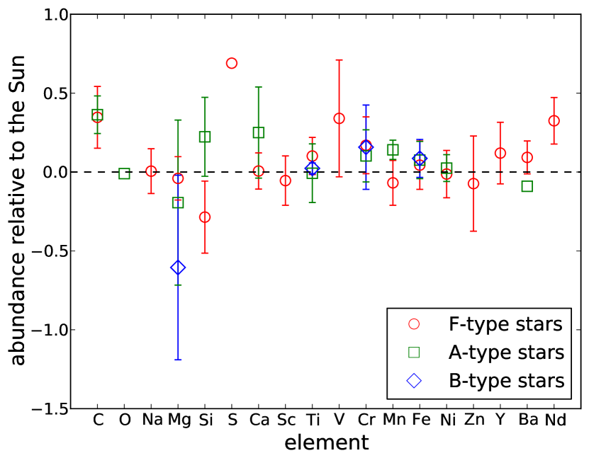
Figure 11: The mean abundances of each element relative to solar for F- (red circles), A-(green squares) and B- (blue diamonds) type stars. The error bars are calculated by taking the standard deviations of the calculated mean abundances.

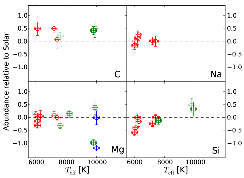
Figure 12: The abundances of C, Na, Mg, and Si relative to the solar abundance (Asplund et al., 2009) against $T_{\rm eff}$. For F- (red circles), A-(green squares) and B- (blue diamonds) type stars.

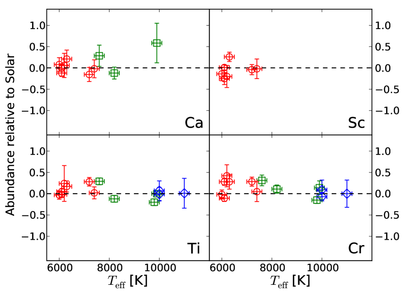
Figure 13: Same as Fig. 12, but for Ca, Sc, Ti and Cr.

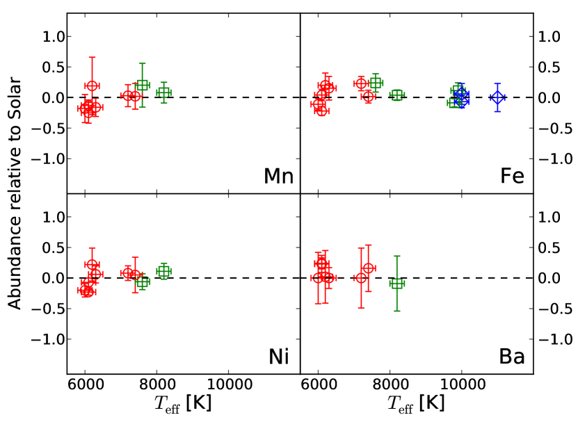
Figure 14: Same as Fig. 12, but for Mn, Fe, Ni and Ba.

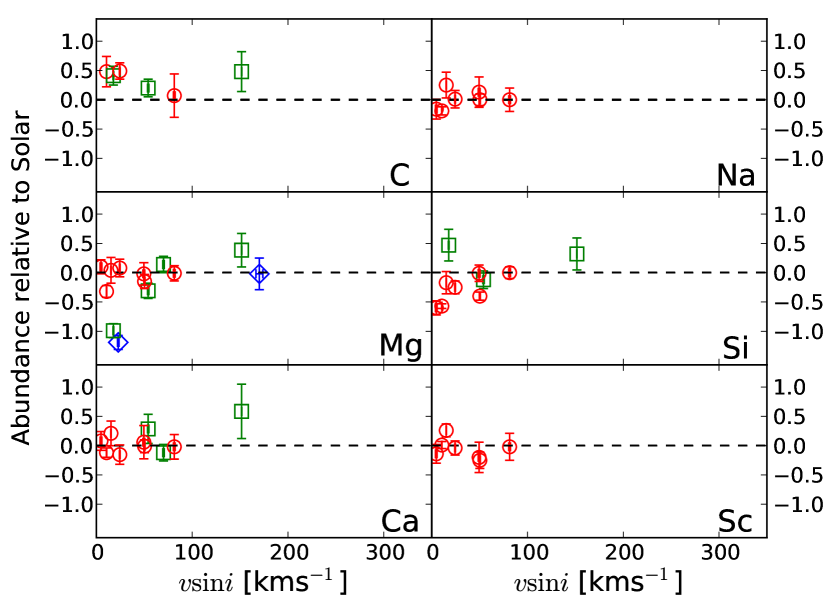
Figure 15: The abundances of C, Na, Mg, Si, Ca and Sc relative to the solar abundance (Asplund et al., 2009) against $v\sin i$. For F- (red circles), A-(green squares) and B- (blue diamonds) type stars.

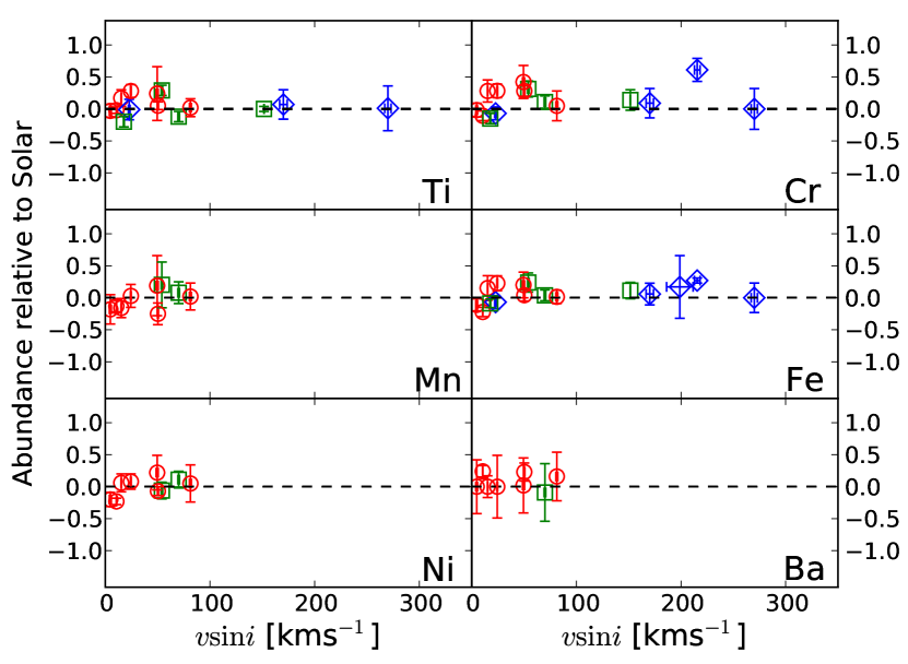
Figure 16: Same as Fig. 15, but for Ti, Cr, Mn, Fe, Ni and Ba.

7.4 Analysis of chemical abundances

Fig. 11 shows the mean abundance of each element obtained for the F-, A- and B-type stars. The error bars are calculated as the standard deviation about the mean abundance. We consider only the measurements from Table 9 with maximum errors smaller than 0.5.

To determine whether there is any correlation with the stellar fundamental parameters, we have compared each set of element abundances with $T_{\rm eff}$, $v\sin i$, $M/$M_⊙ and fractional main-sequence age. In Figs 12–14, we show abundance as a function $T_{\rm eff}$ and in Figs 15 and 16, we show abundance as a function of $v\sin i$. After comparison between abundance and each of the fundamental parameters, we see no statistically significant patterns. This is consistent with the findings of Kılıçoğlu et al. (2016).

In addition, we have compared our results with the previous studies of the open clusters NGC6405, NGC 5460 and Praesape performed by Kılıçoğlu et al. (2016), Fossati et al. (2011a) and Fossati et al. (2007, 2008b, 2010), respectively. This allows us to determine whether there is any evidence for correlation between cluster age and abundance. We compare our results with only these clusters since they have all been analysed within this project, and the analysis has been either fully carried out (Praesape and NGC 5460) or supervised by one of us (LF) (NGC 6405 and NGC 6250), to minimize the possibility of systematic differences between the results. To compare the results from each cluster analysis, we have offset the abundance values of the individual chemical elements according to the cluster metallicities as estimated from Fe abundances of the cluster F and later type stars, which should be less affected by diffusion than earlier type stars.

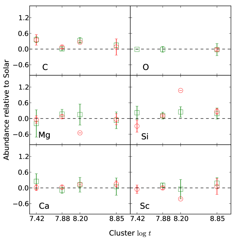
Figure 17: A comparison between the mean C, O, Mg, Si, Ca and Sc abundances found for each of the previous studies and those found in this paper. Mean abundances for F- (red circles) and A-type (green squares) stars are plotted against cluster age ($\log t=7.42$ for NGC 6250; $\log t=7.88$ for NGC 6405; $\log t=8.20$ for NGC5460; and $\log t=8.85$ for Praesepe). The error is given by the standard deviation of all the measured abundances.

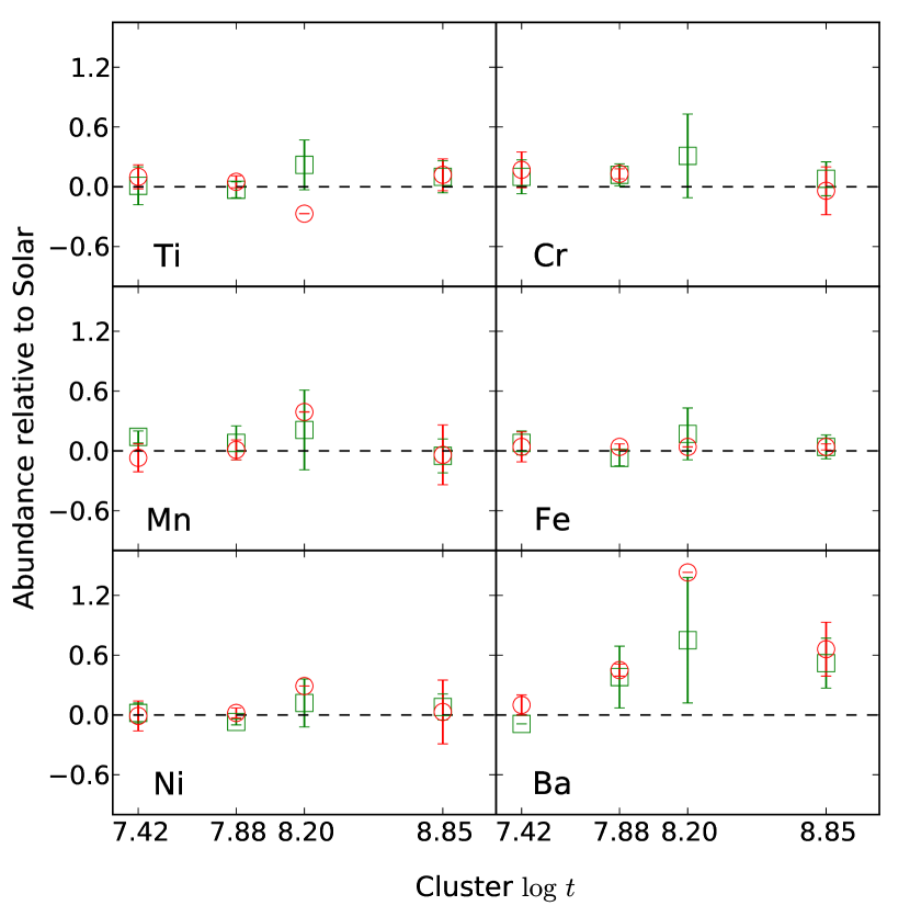
Figure 18: Same as Fig. 18 but for Ti, Cr, Mn, Fe, Ni and Ba.

In NGC 6250, we found that O, Na, Sc, Ti, Cr, Mn, Ni, Zn and Y all have solar abundances within the uncertainties, while S and V are overabundant. These results are consistent with the findings of Fossati et al. (2008b), Fossati et al. (2011a) and Kılıçoğlu et al. (2016) for the Praesepe cluster, NGC 5460 and NGC 6405, respectively (see Figs 17 and 18).

Similarly to what was found by Fossati et al. (2008b), Fossati et al. (2011a) and Kılıçoğlu et al. (2016) in the Praesepe cluster, NGC 5460 and NGC 6405, we have found an overabundance of C in the F- and A-type stars of NGC 6250. However, we do not see any trend with age (see Fig. 17).

For all of the F-type stars, we find a solar abundance of Mg, for the A-type and B-type stars there is an underabundance of Mg; however, there is a large spread in the results and all but two stars have approximately solar abundance, which matches with the results of the previous studies.

In agreement with previous studies, we found that in A-type stars Si is overabundant; however, at odds with previous studies, we found that in F-type stars Si is underabundant. Fig. 12 indicates the presence of a possible correlation between $T_{\rm eff}$ and the Si abundance, though a further analysis reveals that this apparent correlation is not statistically significant.

For all of the F-type stars, we find a solar abundance of Ca that is consistent with the previous results. However, for the A-type stars, we find an overabundance, which is contrary to the findings of the previous studies; the origin of this is unclear.

We measure the abundance of Fe in all of our stars to be approximately solar. For both Mn and Fe, Fossati et al. (2011a) found an increase in abundance with $T_{\rm eff}$, which we do not; this therefore may be the result of an age effect. The narrow $T_{\rm eff}$ range of the stars analysed by Fossati et al. (2008b) for the Praesepe cluster means we are unable to provide any definite conclusions until the remaining clusters are analysed.

We measure an almost solar abundance for Ba, albeit with relatively large uncertainties. This is in contrast with the findings of Fossati et al. (2008b), Fossati et al. (2011a) and Kılıçoğlu et al. (2016) who all report overabundances. To understand each of the results together, we plot the mean abundance of Ba measured for each cluster in Fig. 18. We did not consider the stars HD 122983 and HD 123182 from NGC 5460 because of their apparent chemical peculiarities (Fossati et al., 2011a). From Fig. 18, we obtain a hint of a positive correlation of Ba abundance with age; however, the abundance uncertainties are too large to draw any concrete conclusion. By analysing further clusters we will be able to determine whether this effect is the result of diffusion or the different chemistry of the star-forming region for each cluster.

We measure Nd to be overabundant in four stars; however, the data from previous papers are too sparse to provide any conclusion.

Finally, we have compared our results with the study of chemically peculiar magnetic Ap stars by Bailey et al. (2014). This allows us to examine the differences and similarities between abundance trends of chemically normal and chemically peculiar stars. Bailey et al. (2014) found statistically significant trends between He, Ti, Cr, Fe, Pr and Nd and stellar age. They also found a strong trend between the abundances of Cr and Fe, and $T_{\rm eff}$. For Cr, an underabundance was observed for stars with $T_{\rm eff}\lesssim 7000\,$K, for stars with $T_{\rm eff}\gtrsim 7000\,$K the abundance of Cr sharply rises and peaks at $T_{\rm eff}\sim 10000\,$K before falling back to approximately solar. For Fe, an underabundance was observed for stars with $T_{\rm eff}\lesssim 8000\,$K and an overabundance for the remaining stars. These results are in stark contrast with what we observed for NGC 6250. This suggests that the abundance of chemical elements in the photosphere of chemically normal F-, A- and B-type stars remains relatively constant during their main-sequence lifetime except when influenced by a magnetic field.

8 Conclusions

We have presented the new code for spectral analysis, sparti_simple. Based on cossam_simple, a modified version of the radiative transfer code cossam, sparti_simple employs the inversion algorithm LMA and allows one to recover the abundance of the chemical elements of non-magnetic stellar atmospheres. To test our new code, we have performed the abundance analysis of the Sun, HD 32115 and 21 Peg and compared our results with those previously published in the thorough works by Prsa et al. (2016), Asplund et al. (2009), Fossati et al. (2011b) and Fossati et al. (2009), finding excellent agreement.

We have applied our new code for a spectroscopic study of the open cluster NGC 6250, which was observed with the FLAMES instrument of the ESO VLT. From the observed sample of stars, we have performed cluster membership analysis based on a $K$-means clustering procedure and analysis of the photometry. As a result of our analysis, we selected 19 stars from our sample as members of the cluster. We have computed the cluster mean proper motions of 0.4 $\pm$ 3.0 mas yr^-1 in RA, $-$4.80 $\pm$ 3.2 mas yr^-1 in DEC and radial velocity of $-$10 $\pm$ 6 km s^-1. These values agree within the errors with the values calculated by Kharchenko et al. (2013). The age and distance given by Kharchenko et al. (2013) agree well with our photometric analysis of the cluster.

Finally, we have examined the chemical abundance measurements for each star and searched for any trend between abundance and the stellar fundamental parameters and between the abundance measured in this study and the abundance measured in the previous studies of older clusters by Fossati et al. (2007, 2008b, 2010), Fossati et al. (2011a) and Kılıçoğlu et al. (2016). Our results for the abundance of O, Na, Sc, Ti, Cr, Mn, Ni, Zn and Y are solar within the uncertainties, while S and V are overabundant. These results are consistent with previous studies. We do not find evidence of the correlation between either the Fe or Mn abundance and $T_{\rm eff}$ found by Fossati et al. (2011a); however, this may be evidence of an age effect and we need to study more clusters before being able to determine this. We find hints of an increase in mean Ba abundance with cluster age but more clusters should be analysed to confirm this trend. Comparing our results with those from Bailey et al. (2014), who searched for trends between chemical abundances and stellar parameters of chemically peculiar magnetic Ap stars, suggests that the abundance of chemical elements in the photosphere of chemically normal F-, A- and B- type stars remains relatively constant during their main-sequence lifetime except when influenced by a magnetic field.

References

- Alecian & Stift (2004) Alecian G., Stift M. J., 2004, A&A, 416, 703
- Asplund et al. (2009) Asplund M., Grevesse N., Sauval A. J., Scott P., 2009, ARA&A, 47, 481
- Aster et al. (2013) Aster R. C., Borchers B., Thurber C. H., 2013, Parameter estimation and inverse problems. Elsevier, New York
- Auer et al. (1977) Auer L. H., Heasley J. N., House L. L., 1977, ApJ, 216, 531
- Bagnulo et al. (2006) Bagnulo S., Landstreet J. D., Mason E., Andretta V., Silaj J., Wade G. A., 2006, A&A, 450, 777
- Bailey et al. (2014) Bailey J. D., Landstreet J. D., Bagnulo S., 2014, A&A, 561, A147
- Baschek et al. (1966) Baschek B., Holweger H., Traving G., 1966, Astron. Abh. Hamburger Sternwarte, 8, 26
- Bayer et al. (2000) Bayer C., Maitzen H., Paunzen E., Rode-Paunzen M., Sperl M., 2000, A&AS, 147, 99
- Bischof (2005) Bischof K. M., 2005, Mem. Soc. Astron. Ital. Suppl., 8, 64
- Bressan et al. (2012) Bressan A., Marigo P., Girardi L., Salasnich B., Dal Cero C., Rubele S., Nanni A., 2012, MNRAS, 427, 127
- Chen et al. (2014) Chen Y., Girardi L., Bressan A., Marigo P., Barbieri M., Kong X., 2014, MNRAS, 444, 2525
- Chen et al. (2015) Chen Y., Bressan A., Girardi L., Marigo P., Kong X., Lanza A., 2015, MNRAS, 452, 1068
- Chmielewski (1979) Chmielewski Y., 1979, Spectres stellaires synthetiques : programmes de calcul Chmielewski. L’Observatoire de Geneve
- Dappen et al. (1987) Dappen W., Anderson L., Mihalas D., 1987, ApJ, 319, 195
- Dias et al. (2006) Dias W. S., Assafin M., Flório V., Alessi B. S., Líbero V., 2006, A&A, 446, 949
- Feinstein et al. (2008) Feinstein C., Vergne M. M., Martínez R., Orsatti A. M., 2008, MNRAS, 391, 447
- Fensl (1995) Fensl R. M., 1995, A&AS, 112, 191
- Folsom et al. (2007) Folsom C. P., Wade G. A., Bagnulo S., Landstreet J. D., 2007, MNRAS, 376, 361
- Fossati et al. (2007) Fossati L., Bagnulo S., Monier R., Khan S., Kochukhov O., Landstreet J., Wade G., Weiss W., 2007, A&A, 476, 911
- Fossati et al. (2008a) Fossati L., Bagnulo S., Landstreet J., Wade G., O.Kochukhov Monier R., Weiss W., Gebran M., 2008a, Contrib. Astron. Obs. Skalnate Pleso, 38, 123
- Fossati et al. (2008b) Fossati L., Bagnulo S., Landstreet J., Wade G., O.Kochukhov Monier R., Weiss W., Gebran M., 2008b, A&A, 483, 891
- Fossati et al. (2009) Fossati L., Ryabchikova T., Bagnulo S., Alecian E., Grunhut J., Kochukhov O., Wade G., 2009, A&A, 503, 945
- Fossati et al. (2010) Fossati L., Mochnacki S., Landstreet J., Weiss W., 2010, A&A, 510, A8
- Fossati et al. (2011a) Fossati L., Folsom C. P., Bagnulo S., Grunhut J. H., Kochukhov O., Landstreet J. D., Paladini C., Wade G. A., 2011a, MNRAS, 413, 1132
- Fossati et al. (2011b) Fossati L., Ryabchikova T., Shulyak D. V., Haswell C. A., Elmasli A., Pandey C. P., Barnes T. G., Zwintz K., 2011b, MNRAS, 417, 495
- Gebran & Monier (2008) Gebran M., Monier R., 2008, A&A, 483, 567
- Gebran et al. (2008) Gebran M., Monier R., Richard O., 2008, A&A, 479, 189
- Gebran et al. (2010) Gebran M., Vick M., Monier R., Fossati L., 2010, A&A, 523, 71
- Glazunova et al. (2008) Glazunova L. V., Yushchenko A. V., Tsymbal V. V., Mkrtichian D. E., Lee J. J., Kang Y. W., Valyavin G. G., Lee B.-C., 2008, AJ, 136, 1736
- González-García et al. (2006) González-García B. M., Zapatero Osorio M. R., Béjar V. J. S., Bihain G., Barrado Y Navascués D., Caballero J. A., Morales-Calderón M., 2006, A&A, 460, 799
- Grassitelli et al. (2015) Grassitelli L., Fossati L., Langer N., Miglio A., Istrate A. G., Sanyal D., 2015, A&A, 584, L2
- Gray (2005) Gray D., 2005, The Observation and Analysis of Stellar Photospheres. Cambridge Univ. Press, Cambridge
- Henden et al. (2016) Henden A. A., Templeton M., Terrell D., Smith T. C., Levine S., Welch D., 2016, VizieR Online Data Catalog, 2336
- Herbst (1977) Herbst W., 1977, AJ, 82, 902
- Hubeny & Lanz (1995) Hubeny I., Lanz T., 1995, ApJ, 439, 875
- Hubeny et al. (1994) Hubeny I., Hummer D. G., Lanz T., 1994, A&A, 282, 151
- Hui et al. (1978) Hui A. K., Armstrong B. H., Wray A. A., 1978, J. Quantit. Spectrosc. Radiat. Transfer, 19, 509
- Hummer & Mihalas (1988) Hummer D. G., Mihalas D., 1988, ApJ, 331, 794
- Kharchenko et al. (2013) Kharchenko N. V., Piskunov A. E., Schilbach E., Röser S., Scholz R.-D., 2013, A&A, 558, A53
- Kılıçoğlu et al. (2016) Kılıçoğlu T., Monier R., Richer J., Fossati L., Albayrak B., 2016, AJ, 151, 49
- Kochukhov et al. (2010) Kochukhov O., Makaganiuk V., Piskunov N., 2010, A&A, 524, A5
- Kurucz (1993a) Kurucz R., 1993a, Opacities for Stellar Atmospheres: [+0.0],[+0.5],[+1.0]. Kurucz CD-ROM No. 2. Smithsonian Astrophysical Observatory, Cambridge, MA,
- Kurucz (1993b) Kurucz R., 1993b, ATLAS9 Stellar Atmosphere Programs and 2 km/s grid. Kurucz CD-ROM No. 13. Smithsonian Astrophysical Observatory, Cambridge, MA, 13
- Kurucz (2005) Kurucz R. L., 2005, Mem. Soc. Astron. Ital. Suppl., 8, 14
- Landstreet (2004) Landstreet J. D., 2004, in Zverko J., Ziznovsky J., Adelman S. J., Weiss W. W., eds, Proc. IAU Symp Vol. 224, The A-Star Puzzle. Cambridge Univ. Press, Cambridge, p. 423
- Langer & Kudritzki (2014) Langer N., Kudritzki R. P., 2014, A&A, 564, A52
- Levenberg (1944) Levenberg K., 1944, Q. Appl. Math., 2, 164
- MacQueen (1967) MacQueen J., 1967, in Lucien M. Le Cam and Jerzy Neyman ed., Proceedings of the Fifth Berkeley Symposium on Mathematical Statistics and Probability, Volume 1: Statistics. Univ. California Press, Berkeley, CA,, Berkeley, Calif., p. 281
- Marquardt (1963) Marquardt D. W., 1963, J. Soc. Ind. Appl. Math., 11, 431
- Michaud (1970) Michaud G., 1970, ApJ, 160, 641
- Moffat & Vogt (1975) Moffat A., Vogt N., 1975, A&AS, 20, 155
- Pasquini & et al. (2002) Pasquini L., et al. 2002, The Messenger, 110, 1
- Piskunov et al. (1995) Piskunov N. E., Kupka F., Ryabchikova T. A., Weiss W. W., Jeffery C. S., 1995, A&AS, 112, 525
- Prsa et al. (2016) Prsa A., et al., 2016, AJ, 152
- Rees et al. (1989) Rees D. E., Durrant C. J., Murphy G. A., 1989, ApJ, 339, 1093
- Robichon et al. (1999) Robichon N., Arenou F., Mermilliod J.-C., Turon C., 1999, A&A, 345, 471
- Roeser et al. (2010) Roeser S., Demleitner M., Schilbach E., 2010, AJ, 139, 2440
- Sanders (1971) Sanders W. L., 1971, A&A, 14, 226
- Seaton (1990) Seaton M. J., 1990, BAAS, 22, 844
- Skrutskie et al. (2006) Skrutskie M. F., et al., 2006, AJ, 131, 1163
- Stift (1985) Stift M. J., 1985, MNRAS, 217, 55
- Stift (2000) Stift M., 2000, Peculiar Newsl., 27, 33
- Stift et al. (2012) Stift M., Leone F., Cowley C., 2012, MNRAS, 419, 2912
- Stütz et al. (2006) Stütz C., Bagnulo S., Jehin E., Ledoux C., Cabanac R., Melo C., Smoker J. V., 2006, A&A, 451, 285
- Tang et al. (2014) Tang J., Bressan A., Rosenfield P., Slemer A., Marigo P., Girardi L., Bianchi L., 2014, MNRAS, 445, 4287
- Villanova et al. (2009) Villanova S., Carraro G., Saviane L., 2009, A&A, 504, 845
- Vogt et al. (1987) Vogt S. S., Penrod G. D., Hatzes A. P., 1987, ApJ, 321, 496
- Zacharias et al. (2005) Zacharias N., Urban S. E., Zacharias M. I., Wycoff G. L., Hall D. M., Monet D. G., Rafferty T. J., 2005, AJ, 127, 3043