Monogamy inequalities for entanglement using continuous variable measurements

Abstract

We consider three modes $A$, $B$ and $C$ and derive continuous variable monogamy inequalities that constrain the distribution of bipartite entanglement amongst the three modes. The inequalities hold for all such tripartite states, without the assumption of Gaussian states, and are based on measurements of two conjugate quadrature phase amplitudes $X_{i}$ and $P_{i}$ at each mode $i=A,B$. The first monogamy inequality is $D_{BA}+D_{BC}\geq 1$ where $D_{BA}<1$ is the widely used symmetric entanglement criterion, for which $D_{BA}$ is the sum of the variances of $(X_{A}-X_{B})/2$ and $(P_{A}+P_{B})/2$. A second monogamy inequality is $Ent_{BA}Ent_{BC}\geq\frac{1}{\left(1+(g_{BA}^{(sym)})^{2}\right)\left(1+(g_{BC}^{(sym)})^{2}\right)}$ where $Ent_{BA}<1$ is the EPR variance product criterion for entanglement. Here $Ent_{BA}$ is a normalised product of variances of $X_{B}-g_{BA}^{(sym)}X_{A}$ and $P_{B}+g_{BA}^{(sym)}P_{A}$, and $g_{BA}^{(sym)}$ is a parameter that gives a measure of the symmetry between the moments of $A$ and $B$. We also show that the monogamy bounds are increased if a standard steering criterion for the steering of $B$ is not satisfied. We illustrate the monogamy for continuous variable tripartite entangled states including the effects of losses and noise, and identify regimes of saturation of the inequalities. The monogamy relations explain the experimentally observed saturation at $D_{AB}=0.5$ for the entanglement between $A$ and $B$ when both modes have 50% losses, and may be useful to establish rigorous bounds of correlation for the purpose of quantum key distribution protocols.

I Introduction

Entanglement is the major resource for many applications in quantum information processing. Measurable quantifiers exist to determine the amount of entanglement shared between two separated parties, or subsystems, that we denote $A$ and $B$. According to quantum mechanics, the amount of entanglement that exists between two parties $A$ and $B$ puts a constraint on the amount of entanglement that exists between one of those parties ($B$ say) and a third party, $C$. This fundamental result is called monogamy of entanglement.

If the entanglement between two parties $A$ and $B$ can be quantified, it is useful to be able to place a numerical bound on the quantifiable entanglement between the parties $B$ and $C$. As an example, such relations have application to quantum key distribution, where the amount of bipartite entanglement between two parties gives a measure of the correlation between the bit sequences (and hence the key) that each party possesses. The monogamy relations can thus quantify the security of the information shared between two parties. Monogamy relations may also be useful to understand how the bipartite entanglement can be distributed for various types of multipartite entangled states.

A quantifiable monogamy relation involving the concurrence measure of bipartite entanglement was originally derived for three qubit systems by Coffman, Kundu and Wootters CKW-1 . Since then, the interest in understanding and quantifying monogamy of entanglement has expanded Adesso2012 ; Adesso_Monog2 ; AdessoMonog ; BaiMonEntangFormation ; Masanes2006 ; MonSquareQDiscord ; MR_Monogamy2013 ; osb ; Regula2014StrongMon4Qubit ; Toner ; steeringellipsoids ; ZhuEntMonRelQubit ; newqiadyu ; MonPureQubits . Work by Adesso et al Adesso2012 ; Adesso_Monog2 ; AdessoMonog formulated monogamy relations for systems involving Gaussian states gausadesso and continuous variable measurements. Barrett et al, Masanes et al and Toner et al investigated the monogamy of Bell nonlocality Toner ; Masanes2006 . Monogamy relations for the Einstein-Podolsky-Rosen (EPR) paradox and EPR steering, which are directional forms of nonlocality EPRsteering-1 ; Jones-steering ; rrmp ; MR_EPR ; EPR , have been studied and derived in Refs. MR_Monogamy2013 ; steeringellipsoids ; newqiadyu .

In this paper, we derive entanglement monogamy relations for continuous variable entanglement quantifiers based on Einstein-Podolsky-Rosen (EPR) correlations EPR . The amount of EPR correlation between the field quadrature phase amplitudes $X_{A,B}$ and $P_{A,B}$ of two modes $A$, $B$ can be defined using variances MR_EPR ; TanDuan ; duan ; ent-crit . Often the EPR correlations are as for a two-mode squeezed state, where the correlation is between $X_{A}$ and $X_{B}$, and $P_{A}$ and $-P_{B}$, so that the variances of $X_{A}-X_{B}$ and $P_{A}+P_{B}$ vanish in a limit of perfect entanglement MR_EPR . This limit is thus also a limit of infinite two-mode squeezing. Entanglement can be inferred if the sum of these two variances drops below a critical level ent-crit ; duan ; TanDuan .

Considering the sum of the two variances $D_{AB}=\{(\Delta(X_{A}-X_{B}))^{2}+(\Delta(P_{A}+P_{B}))^{2}\}/4$, the Tan-Duan-Giedke-Cirac-Zoller (TDGCZ) criterion for entanglement is $D_{AB}<1$ TanDuan ; duan . Here we use a scaling of the quadratures so that the uncertainty principle gives $\Delta X_{A}\Delta P_{A}\geq 1$ and $\Delta X_{B}\Delta P_{B}\geq 1$. This criterion has been used in numerous experiments to detect entanglement rrmp . Importantly, it is a symmetric criterion, in that the criterion is unchanged if the labels $A$ and $B$ are exchanged. In this paper, we consider three modes $A$, $B$ and $C$ and derive the monogamy inequality

$$D_{BA}+D_{BC}\geq\max\{1,S_{B|{\{AC\}}}\}$$ (1)

that holds to describe the distribution of the bipartite entanglement for all states, without the assumption of Gaussianity. Here $S_{B|\{AC\}}$ is an EPR steering parameter that certifies steering of mode $B$ by measurements on the combined system $AC$ if $S_{B|\{AC\}}<1$. This steering parameter was used in the experiments described in Ref. rrmp that detected the continuous variable EPR paradox. The relation of Eq. (1) may be useful to establish rigorous bounds of correlation for the purpose of quantum key distribution protocols and also explains the experimentally observed saturation at $D_{AB}=0.5$ by Bowen et al. bowen-exp for the entanglement between $A$ and $B$ when both modes undergo 50% attenuation of intensity .

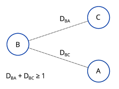
Figure 1: Entanglement monogamy: The entanglement is shared in a way that ensures $D_{BA}+D_{BC}\geq 1$. Here, $D_{AB}$ is a quantifier of symmetric bipartite entanglement between $A$ and $B$. Bipartite entanglement is depicted by the dashed lines. A stricter condition given by Eq. (2) places bounds on the value of the more general entanglement bipartite quantifiers $Ent_{AB}$ and $Ent_{BC}$, in terms of bipartite symmetry parameters $g_{BA}^{(sym)}$ and $g_{BC}^{(sym)}$. The main text shows how stricter conditions apply if steering of system $B$ by the combined systems $AC$ cannot be demonstrated using a standard steering criterion.

It was shown by Duan et al duan and Giovannetti et al ent-crit that a more sensitive entanglement criterion is possible if one considers the variances of $X_{A}+gX_{B}$ and $P_{A}-gP_{B}$, where $g$ are real constants. This leads to a criterion for entanglement of $Ent_{AB}<1$, where $Ent_{AB}$ is defined as a normalised product of the variances of $X_{A}+gX_{B}$ and $P_{A}-gP_{B}$, the $g$ being optimally chosen qiprl ; tele . For an important class of two-mode Gaussian systems, such criteria have been shown to be necessary and sufficient and equivalent to the Peres-Simon Positive-Partial-Transpose (PPT) criterion qiprl ; duan ; Simon . In Section IV of this paper, we derive monogamy relations for this PPT-EPR variance entanglement quantifier. Specifically, we show that

$$Ent_{BA}Ent_{BC}\geqslant\frac{\max{\{1,S_{B|\{AC\}}^{2}\}}}{\left(1+(g_{BA}^{(sym)})^{2}\right)\left(1+(g_{BC}^{(sym)})^{2}\right)}$$ (2)

Here, $g_{BA}^{(sym)}$ and $g_{BC}^{(sym)}$ are symmetry parameters introduced in Refs. qiprl ; tele , which quantify the amount of symmetry between the moments of $B$ and $A$, and $B$ and $C$, respectively. These parameters take the value $g^{(sym)}=1$ when the moments are perfectly symmetrical. It has been explained in the Refs. qiprl ; tele how the effect of thermal noise and dissipation on the different modes can alter the values of the symmetry parameters.

In Sections III and IV, we illustrate the application of the monogamy relations Eqs. (1) and (2) to the tripartite entangled system created using a two-mode squeezed state and a beam splitter trivL . Such tripartite entangled states (or very similar states) have been realised experimentally runyantri ; seiji ; hansmulti ; aoki ; shalm-1 ; threecolourcv . We show that the second inequality (Eq. (2)) is more sensitive and saturates for this tripartite system for all beam splitter couplings, in regimes corresponding to a high squeeze parameter $r$ where the tripartite entanglement is maximised in terms of the underlying EPR correlations. The first relation (Eq. (1)) is useful however for identifying bounds on the symmetric entanglement quantified by $D_{AB}$, which has been shown useful for specific teleportation protocols tele .

We also study the monogamy relations where coupling of the modes to the environment will create additional losses and thermal noise. Such couplings can be asymmetric (hence altering the symmetry parameters) and also lead to a decrease in the amount of EPR steering possible. We are thus able to verify the decrease in overall entanglement when the steering identified by the parameter $S_{A|\{BC\}}$ is diminished. Importantly, we identify regimes of saturation of the monogamy inequality (2), for almost all values of attenuation of the shared mode (depicted by $B$ in Figure 1), if mode $C$ has been created by an eavesdropper using a 50/50 beam splitter to tap mode $A$. This gives a fundamental explanation of the observed optimal value of $D_{BA}=0.5$ measured in the experiment of Bowen et al, for the symmetric case when the mode $B$ has 50% attentuation bowen-exp .

Our derivations are general for three-mode tripartite states $A$, $B$ and $C$ and do not depend on the assumption of Gaussian states gausadesso . The derivations are based on a previous monogamy result for EPR-steering given in reference MR_Monogamy2013 and in fact we find that the steering plays an important role in the monogamy relations. Only if the steering between $B$ and $AC$ is preserved in a specific directional sense is the monogamy bound limited by the quantum noise level. This gives an indication that directional properties of entanglement, such as steering for which the parties are not interchangeable, play an important role in quantum information applications.

II Monogamy of Entanglement using the symmetric TDGCZ criterion

The symmetric Tan-Duan-Giedke-Cirac-Zoller (TDGCZ) criterion for certifying entanglement between two modes is defined in terms of the sum of the Einstein-Podolsky-Rosen variances

$$D_{AB}=\frac{1}{4}\Bigl{(}\mathrm{Var}(X_{A}-X_{B})+\mathrm{Var}(P_{A}+P_{B})\Bigr{)}$$ (3)

and is given as TanDuan ; duan :

$$D_{AB}<1$$ (4)

Here $X_{A},$ $P_{A}$ and $X_{B}$, $P_{B}$ are the quadrature phase amplitudes for modes symbolised by $A$ and $B$ respectively, and $\mathrm{Var}(X)=(\Delta X)^{2}=\langle X^{2}\rangle-\langle X\rangle^{2}$ denotes the variance of $X$. Denoting the boson annihilation operators of each mode by $\hat{a}$ and $\hat{b}$, we have selected $X_{A}=\hat{a}+\hat{a}^{\dagger}$, $P_{A}=(\hat{a}-\hat{a}^{\dagger})/i,$ $X_{B}=\hat{b}+\hat{b}^{\dagger}$ and $P_{B}=(\hat{b}-\hat{b}^{\dagger})/i$ for which the uncertainty relation is $\Delta X\Delta P\geq 1$.

The criterion $D_{AB}<1$ is sufficient (though not necessary) to detect entanglement for all two-mode states, regardless of assumptions about the nature of the two-mode state. Nonetheless, for two-mode Gaussian symmetric fields where the moments of fields $A$ and $B$ are equal, the entanglement criterion can be shown necessary and sufficient for two-mode entanglement for some choice of quadrature phase amplitudes $X$ and $P$ (defined by a phase angle $\theta$) duan ; Simon .

Result (1): The first main result of the paper is that for any three modes $A$, $B$ and $C$, the following monogamy relation holds:

$$D_{BA}+D_{BC}\geq 1$$ (5)

The proof is given in the Appendix and is based on an earlier result for monogamy of steering MR_Monogamy2013 . The relation holds for all three-mode quantum states. In particular, the relation does not rely on the assumption of Gaussian states.

The monogamy relation (5) has an inherent asymmetry with respect to $B$ and the remaining two systems $A$ and $C$. This asymmetry is depicted in the Fig. (1). In fact, we notice that it is possible to prove a result relating the entanglement sharing to a steering parameter $S_{B|\{AC\}}$ for the steering of the system $B$ by the composite system $AC$. We introduce the steering parameter as $S_{A|B}$ as follows. A sufficient condition to demonstrate steering of $B$ (by measurements made on $A$) is MR_EPR

$$S_{B|A}<1$$ (6)

where the steering parameter $S_{B|A}$ is defined as

$$S_{B|A}=\Delta(X_{B}-g_{x}X_{A})\Delta(P_{B}+g_{p}P_{A})<1$$ (7)

Here $g_{x}$ and $g_{p}$ are real constants chosen to minimise the value of $S_{B|A}$. The condition becomes necessary and sufficient for two-mode Gaussian states, if $g_{x}$ and $g_{p}$ and the choice of quadrature phase amplitudes $X$, $P$ are optimised Jones-steering ; Wisemansteering ; gaussteer . The steering parameter can be more generally defined as rrmp

$$S_{B|A}=\Delta_{inf}X_{B|A}\Delta_{inf}P_{B|A}$$ (8)

where

$$[\Delta_{inf}(X_{B}|X_{A})]^{2}=\sum_{x_{A}}P(x_{A})\sum_{x_{B}}P(x_{B}|x_{A})(x_{B}-\mu_{B|x_{A}})^{2}$$ (9)

is the average conditional variance for $X_{B}$ given the measurement $X_{A}$ at $A$. The $\{x_{A}\}$ is the set of all possible outcomes for $X_{A}$ and $\mu_{B|x_{A}}$ is the mean of $P(X_{B}|X_{A}=x_{A})$. The $\Delta_{inf}X_{B|A}$ is taken as the minimum value of $\Delta_{inf}(X_{B}|X_{A})$ over all possible choices of measurement $X_{A}$ that can be made at $A$. The results of this paper hold for both definitions of $S_{B|A}$, as is apparent from the proofs given in the Appendix. For the example of two-mode Gaussian states, the definitions become equivalent rrmp .

The next result indicates that the distribution of the entanglement as detected by the $D_{AB}$ parameter in accordance with inequality (5) can only be optimised if steering exists between the system $B$ and the composite system $AC.$

Result (2): The following inequality holds:

$$D_{BA}+D_{BC}\geq\max{\{1,S_{B|\{AC\}}\}}$$ (10)

The proof is given in the Appendix. For this inequality, it is necessary to ensure that the measured steering parameter is the optimal one, obtained by optimising the values of $g_{x}$ and $g_{p}$ and the choice of quadrature phase angle for the inference of $B$. For this reason, the second definition (8) involving the conditional variances is generally more useful, where care is taken to ensure the conditional variances are defined for the choice of quadratures at both $A$ and $C$ that minimise the conditional variance.

The monogamy inequality (10) relates the TDGCZ entanglement to the value of the steering parameter $S_{B|\{AC\}}$. If the noise levels are such that there is no steering of $B$ by the composite system $AC$ detectable by $S_{B|\{AC\}}<1$, then the amount of entanglement is reduced. The monogamy relation states that the lower bound $D_{BA}+D_{BC}=1$ can only be reached if there is steering of $B$ by the composite system $AC$. Otherwise the monogamy is restricted by the value of the steering parameter.

III Illustration of Monogamy for tripartite CV entangled systems

The relations given by Results (1) and (2) can be verified experimentally and are useful to explain past experimental observations. We consider the continuous variable (CV) tripartite system generated by placing squeezed vacuum inputs through a series of beam splitters, or else via nondegenerate down conversion followed by a beam splitter on one mode, as shown in the diagram of Fig. 2 trivL . At the output of the device are three modes, that we label $A$, $B$ and $C$.

The essential feature is that a two-mode squeezed state is first generated for two modes that we label $A$ and $F$. The two-mode squeezing corresponds to an EPR entanglement between modes $B$ and $F$, which can be generated as the outputs of a beam splitter $BS1$ with squeezed vacuum inputs, or else via a parametric down conversion (PDC) process rdprl . The amount of entanglement (two-mode squeeing) between the two modes $B$ and $F$ is determined by the two-mode squeezing parameter . The amount of entanglement increases as $r$ increases MR_EPR . The mode $F$ is then coupled to a second beam splitter $BS2$ which has two output modes, $A$ and $C$. The transmission efficiency for $A$ is given by $\eta_{0}$; that for $C$ is therefore $1-\eta_{0}$. The second input to the beam splitter $BS2$ is a vacuum state trivL .

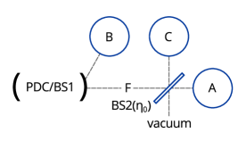
Figure 2: Configuration for the generation of a tripartite entangled system. Here, a two-mode squeezed state is generated using a parametric down conversion (PDC) process. Similar two-mode entanglement can be created using single mode squeezed vacuum states that are input to a beam splitter $BS1$. Either way, entangled modes $B$ and $F$ are created at the outputs of the first device. The entanglement between $F$ and $B$ is determined by a squeeze parameter $r$. Final modes $A$ and $C$ are created at the output of the second beam splitter $BS2$ which has a transmission efficiency $\eta_{0}$ and second vacuum input. The resulting three modes $B$, $A$ and $C$ are genuinely tripartite-entangled.

The two-mode entanglement between modes $B$ and $F$ can be modelled as that of a two-mode squeezed state, given as the output of a parametric down conversion MR_EPR . The nonzero covariance matrix elements in this case are denoted $n=\langle X_{B}^{2}\rangle$, $m=\langle X_{F}^{2}\rangle$ and $c=\langle X_{B}X_{F}\rangle$ where here $\langle X_{F}\rangle=\langle P_{F}\rangle=..=0$ and the solutions for the two-mode squeezed state are $n=\cosh 2r$, $m=\cosh 2r$ and $c=\sinh(2r)$. We see that $[\Delta(X_{B}-X_{F})]^{2}=[\Delta(P_{B}+P_{F})]^{2}=n-2c+m$. The mode $F$ is then input to a beam splitter with transmission efficiency $\eta_{0}$ (Fig. 2) and we see that the two-mode entanglement between $B$ and $A$ is calculated by defining A as the beam $F$ transmitted with efficiency $\eta_{0}$.

We now test the relation of Result (1) for the three output modes, specified in the diagram of Figure 2 by $A$, $B$ and $C$. The beam splitter coupling is given by a unitary transformation, and we evaluate the correlation between $B$ and $A$ in terms of $\eta_{0}$ and $r$ by tracing over the mode $C$ where the beam splitter transmission efficiency for $A$ is given by $\eta_{0}$. Similarly, for the calculation of $D_{BC}$ the mode $C$ is evaluated by tracing over the mode $A$. The beam splitter efficiency for the transmission of the field $C$ is $1-\eta_{0}$. The covariances become

$$n_{BA} = \cosh 2r$$

$$m_{BA} = \eta_{0}\cosh 2r+\left(1-\eta_{0}\right)$$

$$c_{BA} = \sqrt{\eta_{0}}\sinh 2r$$ (11)

and those for modes $B$ and $C$ are obtained by replacing $\eta_{0}$ with $1-\eta_{0}$. Hence

$$D_{BA} = (n_{BA}-2c_{BA}+m_{BA})/2$$ (12)

$$= \Bigl{(}\eta_{0}\cosh 2r+\left(1-\eta_{0}\right)+\cosh 2r$$

$$-2\sqrt{\eta_{0}}\sinh 2r\Bigr{)}/2$$

and

$$D_{BC} = \Bigl{(}(1-\eta_{0})\cosh 2r+\eta_{0}+\cosh 2r$$ (13)

$$-2\sqrt{1-\eta_{0}}\sinh 2r\Bigr{)}/2$$

We notice from the expression of $D_{BA}$ that $D_{BA}\leq 1$ for all $r$ when $\eta_{0}=1$. For larger $r$, $D_{BA}$ exceeds $1$ for smaller $\eta_{0}$ values. The monogamy relation of Result (1) is illustrated in Figure 3 for the configuration of Figure 2 where the modes $B$ and $F$ are generated as a two-mode squeezed state. Figure 3 plots the values of $D_{BA}$, $D_{BC}$ and $D_{BA}+D_{BC}$ for various $\eta_{0}$. We note the relation is verified, but that saturation (achieved when the equality $D_{BA}+D_{BC}=1$ is reached) does not occur.

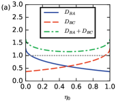
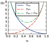
Figure 3: Monogamy for the tripartite state of Figure 2 with no extra losses or noise present. The $D_{BA}$, $D_{BC}$ and $D_{BA}+D_{BC}$ versus $\eta_{0}$ for the state of Figure 2. Here $r=0.5$ (a) and $r=2$ (b). The monogamy bound of $1$ is indicated by the gray dotted line.

To test the relation of Result (2), we need to consider the steering of $B$. The value of the steering parameter $S_{B|F}$ is minimized to

$$S_{B|F} = \left(n_{BF}-c_{BF}^{2}/m_{BF}\right)$$ (14)

using the optimal factors $g_{x}=c_{BF}/m_{BF}$, $g_{p}=c_{BF}/m_{BF}$. Thus, the steering parameter is MR_EPR

$$S_{B|\{AC\}}=1/\cosh(2r)$$ (15)

which cannot exceed $1$ for any $r$. The smallness of the steering parameter gives a measure of the degree of the steering. The steering parameter $S_{B|\{AC\}}$ is evaluated as $0$ for large $r$ by noting that the full knowledge of quadrature phase amplitudes of both $A$ and $C$ enables prediction of the amplitudes at $B$. This type of collective steering was examined in Ref. genepr . Hence the sum $D_{BA}+D_{BC}$ is bounded below by the quantum noise level given by $1$. The Result (2) will be verified in Sections III.B and C for different scenarios.

III.1 Extra losses for the shared mode $B$

We can model the effects of extra loss for mode $B$, by coupling the mode $B$ to an imaginary beam splitter ($BS3$). This widely-used method ys models loss that occurs after the interaction that creates the two-mode squeezing. The final detected mode at the site $B$ is modelled as the output transmitted mode from the imaginary beam splitter $BS3$ (which for simplicity we also denote by $B$). We model the overall loss for the mode $B$ by the transmission efficiency $\eta_{B}$. Thus, we find the new covariances describing the two-mode entanglement between $F$ and $B$ to be

$$n_{BF} = \eta_{B}\cosh 2r+\left(1-\eta_{B}\right)$$

$$m_{BF} = \cosh 2r$$

$$c_{BF} = \sqrt{\eta_{B}}\sinh 2r$$ (16)

The modes $A$ and $C$ are created by the beam splitter $BS2$ coupled to mode $F$ as in the diagram of Figure 2. Here, extra losses created for the output modes $A$ and $C$ are ignored, for the sake of simplicity. We then solve for the final covariances. Denoting $n_{BA}=\langle X_{B}^{2}\rangle$, $m_{BA}=\langle X_{A}^{2}\rangle$ and $c_{BA}=\langle X_{B}X_{A}\rangle$ where here $\langle X_{A}\rangle=\langle P_{A}\rangle=..=0$, we find

$$n_{BA} = \eta_{B}\cosh 2r+\left(1-\eta_{B}\right)$$

$$m_{BA} = \eta_{0}\cosh 2r+\left(1-\eta_{0}\right)$$

$$c_{BA} = \sqrt{\eta_{0}}\sqrt{\eta_{B}}\sinh 2r$$ (17)

Hence

$$D_{BA} = (n_{BA}-2c_{BA}+m_{BA})/2$$ (18)

$$= \Bigl{(}\eta_{B}\cosh 2r+\left(1-\eta_{B}\right)+\eta_{0}\cosh 2r$$

$$+(1-\eta_{0})-2\sqrt{\eta_{B}}\sqrt{\eta_{0}}\sinh 2r\Bigr{)}/2$$

Similarly, evaluating the entanglement between modes $B$ and the second output $C$ of the $BS2$, we replace the transmission $\eta_{0}$ by $1-\eta_{0}$, to obtain

$$D_{BC} = \Bigl{(}\eta_{B}\cosh 2r+1-\eta_{B}+(1-\eta_{0})\cosh 2r$$ (19)

$$+\eta_{0}-2\sqrt{\eta_{B}}\sqrt{1-\eta_{0}}\sinh 2r\Bigr{)}/2$$

We note that if $\eta_{0}=0.5$, then

$$D_{BA}=D_{BC} = \Bigl{(}\eta_{B}\cosh 2r+1-\eta_{B}+0.5+0.5\cosh 2r$$ (20)

$$-2\sqrt{\eta_{B}}\sqrt{0.5}\sinh 2r\Bigr{)}/2$$

which when $\eta_{B}=0.5$ becomes

$$D_{BA}=D_{BC}=0.5\left(1+e^{-2r}\right)$$ (21)

We see that $D_{BA}=D_{BC}$ for $\eta_{0}=0.5$, independent of the value of $r$ and $\eta_{B}$. For $\eta_{0}=\eta_{B}=0.5$, $D_{BA}=D_{BC}\approx 0.5$ in the highly entangled (or squeezed) limit, $r\rightarrow\infty$ bowen-exp .

To test the relation of Result (2), we would need to consider where the steering of $B$ is not possible, so that $S_{B|\{AC\}}>1$. The value of the steering parameter $S_{B|F}$ is minimized to $S_{B|F}=\left(n_{BF}-c_{BF}^{2}/m_{BF}\right)$ using the optimal factors $g_{x}=c_{BF}/m_{BF}$, $g_{p}=c_{BF}/m_{BF}$. Thus, the steering parameter is rrmp

$$S_{B|\{AC\}}=\eta_{B}\cosh 2r+(1-\eta_{B})-\eta_{B}\sinh^{2}(2r)/\cosh(2r)$$ (22)

which cannot exceed $1$ for any $r$.

III.1.1 Bounds on the potential eavesdropper $C$ where modes $A$ and $B$ are lossy: $\eta_{B}=\eta_{0}$

We next analyse the special case of $\eta_{B}=\eta_{0}$. This is the situation where modes $A$ and $B$ are known to have an equal amount of attenuation. This situation is what two observers (one at each mode) may typically assume after transmission of an entangled state so that the modes $A$ and $B$ are spatially separated. The aim is to understand limitations imposed on the entanglement between $B$ and a third mode $C$, based on the motivation that mode $C$ might have been created, or be accessible, by an eavesdropper (Eve). The value of $D_{BA}$ can be measured by observers at modes $A$ and $B$, and that value gives the restriction on $D_{BC}$ based on the monogamy relation $D_{BA}+D_{BC}\geq 1$.

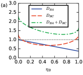
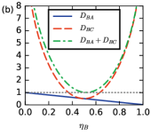
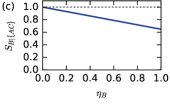
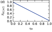
Figure 4: Monogamy for the tripartite state of Figure 2 with equal observed losses for modes $B$ and $A$ ($\eta_{B}=\eta_{0}$). The $D_{BA}$, $D_{BC}$ and $D_{BA}+D_{BC}$ versus $\eta_{0}$ where mode $B$ has loss $\eta_{B}=\eta_{0}$. Here $r=0.5$ (left) and $r=2$ (right). The plot (b) shows the saturation ($D_{BA}+D_{BC}=1$) of the monogamy relation (5) that occurs for large $r$ at $\eta_{0}=0.5$ in this case. See text for explanation. The monogamy bound of $1$ is indicated by the gray dotted line. The steering parameter $S_{B|\{AC\}}$ is plotted for $r=0.5$ (c), and for $r=2$ (d). Steering of $B$ occurs when $S_{B|\{AC\}}<1$.

Letting $\eta_{B}=\eta_{0}$, we obtain the actual solutions for this case where the state is generated as in Figure 2:

$$D_{BA} = 1+\eta_{B}\left(e^{-2r}-1\right)$$

$$D_{BC} = \left(\cosh 2r+1-2\sqrt{\eta_{B}(1-\eta_{B})}\sinh 2r\right)/2$$ (23)

Figure 4 plots the values of $D_{BA}$, $D_{BC}$ and $D_{BA}+D_{BC}$ for various $\eta_{B}=\eta_{0}$. From the expression $D_{BA}$, we see that $D_{BA}\leq 1$ for all $r$, implying that entanglement is preserved between $A$ and $B$ for all attenuation values $\eta$. However, the value of entanglement between $B$ and $C$ as measurable by $D_{BC}$ is limited by the monogamy result $D_{BC}+D_{BA}\geq 1$, as verified by the Figure 4 which gives the specific values for this particular scenario.

The plot Figure 4b show the saturation of the inequality (5) at large entanglement ($r\rightarrow\infty$) to obtain $D_{BA}+D_{BC}=1$ for the tripartite configuration when $\eta_{B}=\eta_{0}=0.5$. This occurs where the modes have symmetric moments, each being subject to an equal attenuation. We note that the monogamy result explains the experimental observation by Bowen et al of a 50% reduction in the value of $D_{BA}$ for the two-mode system where the modes $B$ and $A$ each have a 50% attenuation.

III.1.2 Symmetric tripartite states and asymmetrical attenuation $\eta_{B}\rightarrow 0$

The plots of Figure 5 illustrate the case where there is symmetry between modes $A$ and $C$ so that $\eta_{0}=0.5$, but where the attenuation for mode $B$ is varied. This implies a variable transmission efficiency $\eta_{B}$. In this case, the steering parameter satisfies $S_{B|\{AC\}}<1$, as shown by Eq. (22). Also, $D_{BA}=D_{BC}$. The value of $D_{BA}=D_{BC}$ reduces below $1$ only for a regime where $\eta_{B}\sim\eta_{0}$. This does not imply that there is no bipartite entanglement however, as will be evident in Section IV where a more sensitive entanglement criterion is used.

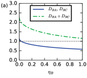
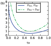
Figure 5: Monogamy for the symmetric tripartite state of Figure 2 where $\eta_{0}=0.5$ and with extra losses for mode $B$. The $D_{BA}$, $D_{BC}$ and $D_{BA}+D_{BC}$ versus $\eta_{B}$, the detection efficiency for mode $B$. Here $r=0.5$ (left) and $r=2$ (right). Always, for these parameters, $D_{BA}=D_{BC}$. The monogamy bound of $1$ is indicated by the gray dotted line.

III.2 Extra loss for modes $A$ and $C$

To test the relation of Result (2), we need to consider scenarios where steering of $B$ as detected by $S_{B|\{AC\}}$ is not possible, so that $S_{B|\{AC\}}>1$. This can be done by placing thermal noise on the mode $B$ qitherm ; laurajosa , or else by adding additional losses to the modes $A$ and $C$ murrayloss ; rrmp . Without loss or extra thermal noise, $S_{B|\{AC\}}$ becomes zero in the limit of large $r$. The smallness of the steering parameter gives a measure of the degree of the steering.

In this Section, we test the monogamy relation of Result (2) by adding losses to modes $A$ and $C$. The extra loss on mode $A$ is modelled by a beam splitter $BS4$ wth transmission (or detection) efficiency $\eta_{A}$. The beam splitter has two inputs, mode $A$ and a second mode that is in a vacuum state (denoted by boson operator $a_{vac}$). The relevant detected moments after loss are then modelled by those of the transmitted mode, with boson operator $a_{det}=\sqrt{\eta_{A}}a+\sqrt{1-\eta_{A}}a_{vac}=\sqrt{\eta_{A}}(\sqrt{\eta_{0}}a+\sqrt{1-\eta_{0}}a_{0,vac})+\sqrt{1-\eta_{A}}a_{vac}$. The covariances become:

$$n_{BA} = \cosh 2r$$

$$m_{BA} = \eta_{0}\eta_{A}\cosh 2r+1-\eta_{0}\eta_{A}$$

$$c_{BA} = \sqrt{\eta_{A}\eta_{0}}\sinh 2r$$ (24)

Similarly, if the extra losses for mode $C$ are modelled similarly by a transmission efficiency $\eta_{C}$, the covariances become (replacing $\eta_{0}$ with $1-\eta_{0}$)

$$n_{BC} = \cosh 2r$$

$$m_{BC} = (1-\eta_{0})\eta_{C}\cosh 2r+1-(1-\eta_{0})\eta_{C}$$

$$c_{BC} = \sqrt{\eta_{C}(1-\eta_{0})}\sinh 2r$$ (25)

Hence

$$D_{BA} = (n_{BA}-2c_{BA}+m_{BA})/2$$ (26)

$$= \Bigl{(}\eta_{0}\eta_{A}\cosh 2r+\left(1-\eta_{0}\eta_{A}\right)+\cosh 2r$$

$$-2\sqrt{\eta_{0}\eta_{A}}\sinh 2r\Bigr{)}/2$$

and

$$D_{BC} = \Bigl{(}(1-\eta_{0})\eta_{C}\cosh 2r+1-\eta_{C}+\eta_{0}\eta_{C}+\cosh 2r$$ (27)

$$-2\sqrt{\eta_{C}(1-\eta_{0})}\sinh 2r\Bigr{)}/2$$

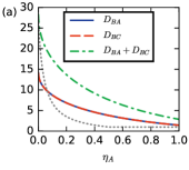
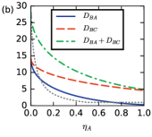
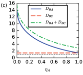
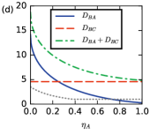
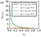
Figure 6: Monogamy for the tripartite state of Figure 2 with extra losses for modes $A$ and $C$. The $D_{BA}$, $D_{BC}$ and $D_{BA}+D_{BC}$ versus $\eta_{A}$ ($\eta_{B}=1$, $r=2$). The monogamy bound is shown by the gray dotted line. Plots (a) and (b) assume $\eta_{A}=\eta_{C}$ and $\eta_{0}=0.5$ (a) and $\eta_{0}=0.8$ (b). Plots (c) and (d) shows values for $\eta_{C}=1$. Plot (e) gives the steering parameter $S_{B|\{AC\}}$ (Eq. (30)) in each case. The $S_{B|\{AC\}}$ is independent of $\eta_{0}$.

The steering parameter is changed by the attenuation of modes $A$ and $C$. The inference of the quadrature phase amplitudes of $B$ by amplitudes $A$ and $C$ cannot be better than the inference made by measurements of amplitudes of $F$. The quadrature amplitudes of $F$ can be determined from those of $A$ and $C$ in a lossless situation as described above. The total effective intensity of mode $F$ can be summed as the intensity of modes $A$ and $C$. The total transmitted intensity (in units of photon number) with the loss present is given by $\eta_{0}\eta_{A}+(1-\eta_{0})\eta_{C}$. The lowest possible value for the steering $S_{B|\{AC\}}$ in the presence of loss for modes $A$ and $C$ is thus given as the steering parameter $S_{B|F}$ where mode $F$ is attenuated by the transmission factor

$$\eta_{F}=\eta_{0}\eta_{A}+(1-\eta_{0})\eta_{C}$$ (28)

The solution is given in Refs. rrmp ; murrayloss . We find

$$S_{B|F} = 1-\eta_{B}\frac{\left[\cosh\left(2r\right)-1\right]\left[2\eta_{F}-1\right]}{\left[1-\eta_{F}+\eta_{F}\cosh\left(2r\right)\right]}\,$$ (29)

where $\eta_{F}$ is the transmission efficiency for mode F and $\eta_{B}$ is that for mode $B$. Here we take $\eta_{B}=1$ so that

$$S_{B|F} = 1-\frac{\left[\cosh\left(2r\right)-1\right]\left[2\eta_{F}-1\right]}{\left[1-\eta_{F}+\eta_{F}\cosh\left(2r\right)\right]}\,$$ (30)

As summarised in Ref. rrmp , $S_{B|F}<1$ for all $\eta_{F}>0.5$, given that $\eta_{B},r\neq 0$. For $\eta_{F}\leq 0.5$, it is possible to obtain $S_{B|F}\geq 1$. Figure 6 demonstrates the monogamy relation for both regimes, where we assume $\eta_{A}=\eta_{C}$. In Figures 6 (a) and (b), the extra losses for modes $A$ and $C$ are assumed equal: $\eta_{A}=\eta_{C}$. The steering parameter exceeds $1$ in that case when $\eta_{F}=\eta_{A}<0.5$ (Figure 6 (e)). In Figure 6 (c) and (d) we assume no extra loss on the mode $C$, modelling a best possible scenario for an eavesdropper who has access to mode $C$. We see that the eavesdropper does not gain access to the symmetric form of entanglement that is indicated by $D_{BC}<1$.

III.3 Squeezed thermal two-mode state

In this Section, we test the monogamy relation by adding thermal noise $n_{B}$ on the mode $B$. This can be done in several ways, depending on what model is used for the creation of the thermal noise. The simplest procedure is to assume that the modes $B$ and $F$ are initially thermally excited states, and then coupled to the interaction that generates the two-mode squeezing discordnoise . The entanglement that is formed between the modes $B$ and $F$ is then modified by the inclusion of the two thermal reservoirs, with thermal excitation numbers given by $n_{a}$ and $n_{b}$ respectively. This might also serve as a simple model for mixed states in optical systems (where thermal noise is negligible at room temperature). The covariance elements of the entangled outputs modes $B$ and $F$ of a squeezed thermal state are discordnoise :

$$n_{BF} = (n_{F}+n_{B}+1)\cosh(2r)+(n_{B}-n_{F})$$

$$m_{BF} = (n_{F}+n_{B}+1)\cosh(2r)-(n_{B}-n_{F})$$

$$c_{BF} = (n_{F}+n_{B}+1)\sinh(2r)$$ (31)

We will take $n_{th}=n_{F}=n_{B}$. The steering parameter becomes in that case

$$S_{B|\{AC\}} = n_{BF}-c_{BF}^{2}/m_{BF}$$ (32)

$$= \left(2n_{th}+1\right)/\cosh 2r$$

and can be shown to exceed $1$ for any given $r,$ for sufficient thermal noise.

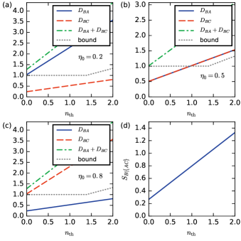
Figure 7: Monogamy relations with thermal noise present: Plots of $D_{BA}$ given by Eq. (LABEL:eq:dbath), $D_{BC}$ given by Eq. (LABEL:eq:dbcth), and $D_{BA}+D_{BC}$ as for Figure 2 with $\eta_{B}=1$ and $r=1$. Graphs give curves versus $\eta_{th}$ for various $\eta_{0}$ where we take $n_{th}=n_{F}=n_{B}$. The monogamy bound given by $\max{\{1,S_{B|\{AC\}}\}}$ is given by the gray dotted curve. Here $S_{B|\{AC\}}$ is given by Eq. (32) as shown in (e). The value of $\eta_{0}$ is $0.2$ (a), $0.5$ (b), $0.8$ (c).

The modes $A$ and $C$ are created by the beam splitter $BS2$ with transmission $\eta_{0}$. We find that $\langle X_{B}^{2}\rangle$ is unchanged, and thus $n_{BA}=n_{BF}$. However, $\langle X_{B}X_{A}\rangle=\langle X_{B}(\sqrt{\eta_{0}}X_{F}+\sqrt{(1-\eta_{0})}X_{vac})\rangle$ where $X_{vac}$ is the quadrature operator from the uncorrelated vacuum input. Also, $\langle X_{A}^{2}\rangle=\langle(\sqrt{\eta_{0}}X_{F}+\sqrt{(1-\eta_{0})}X_{vac})^{2}\rangle$ and thus $\langle X_{A}^{2}\rangle=\eta_{0}\langle X_{F}^{2}\rangle+1-\eta_{0}$. Hence

$$n_{BA} = (n_{F}+n_{B}+1)\cosh(2r)+(n_{B}-n_{F})$$

$$m_{BA} = \eta_{0}(n_{F}+n_{B}+1)\cosh(2r)$$

$$\ \ \ \ \ -\eta_{0}(n_{B}-n_{F})+1-\eta_{0}$$

$$c_{BA} = \sqrt{\eta_{0}}(n_{F}+n_{B}+1)\sinh(2r)$$ (33)

and the covariances $n_{BC}$, $m_{BC}$ and $c_{BC}$ are obtained from those for $BA$ by replacing $\eta_{0}$ with $1-\eta_{0}$. The solutions give

$$D_{BA} = \frac{1}{2}\left(n_{BA}+m_{BA}-2c_{BA}\right)$$

$$= \frac{1}{2}\left[\left(n_{B}+n_{F}+1\right)\cosh 2r+\left(n_{B}-n_{F}\right)\right.$$

$$+\eta_{0}\left(n_{B}+n_{F}+1\right)\cosh 2r-\eta_{0}\left(n_{B}-n_{F}\right)$$

$$\left.+\left(1-\eta_{0}\right)-2\sqrt{\eta_{0}}\left(n_{F}+n_{B}+1\right)\sinh 2r\right]$$

The covariance elements for mode $B$ and $C$ are $n_{BC}=\left(n_{B}+n_{F}+1\right)\cosh 2r+\left(n_{B}-n_{F}\right)$, $m_{BC}=\left(1-\eta_{0}\right)\left(n_{F}+n_{B}+1\right)\cosh 2r-\left(1-\eta_{0}\right)\left(n_{B}-n_{F}\right)+\eta_{0}$ and $c_{BC}=\sqrt{1-\eta_{0}}\left(n_{F}+n_{B}+1\right)\sinh 2r$. $D_{BC}$ is then

$$D_{BC} = \frac{1}{2}\left(n_{BC}+m_{BC}-2c_{BC}\right)$$

$$= \frac{1}{2}\left[\left(n_{B}+n_{F}+1\right)\cosh 2r+\left(n_{B}-n_{F}\right)\right.$$

$$+\left(1-\eta_{0}\right)\left(n_{F}+n_{B}+1\right)\cosh 2r$$

$$-\left(1-\eta_{0}\right)\left(n_{B}-n_{F}\right)+\eta_{0}$$

$$-2\sqrt{1-\eta_{0}}\left(n_{F}+n_{B}+1\right)\sinh 2r$$

The Figure 7 gives plots of the $D_{BA}$, $D_{BC}$ and the steering parameter $S_{A|\{BC\}}$, given in Eq. (32), with different noise values to validate the monogamy relation of Result (2).

IV Monogamy relations for a more general entanglement quantifier

The monogamy relations for the symmetric criterion $D_{AB}$ are useful, since resources satisfying $D_{AB}<1$ are often required for certain protocols tele . However, with the motivation to obtain more sensitive monogamy relations, we next derive relations for the more general entanglement quantifier that has been shown necessary and sufficient for detecting the two-mode entanglement of Gaussian resources.

An entanglement criterion considered by Giovannetti et al is ent-crit

$$Ent_{AB}(\mathbf{g_{AB}})<1$$ (36)

where we define

$$Ent_{AB}(g_{AB})=\frac{\Delta(X_{A}-g_{AB,x}X_{B})\Delta(P_{A}+g_{AB,p}P_{B})}{(1+g_{AB,x}g_{AB,p})}$$ (37)

The $g_{AB}=(g_{AB,x},g_{AB,p})$ where $g_{AB,x}$, $g_{AB,p}$ are real constants that can be optimally chosen to minimize the value of $Ent_{AB}(\mathbf{g_{AB}})$. This minimum value is denoted $Ent_{AB}$ and it has been shown previously that $Ent_{AB}=Ent_{BA}$ qiprl . This is seen by noting that $Ent_{AB}(g_{AB})=Ent_{BA}(1/g_{AB})$ and we will see below that the optimal $g_{AB}$ written as $g_{AB}^{(sym)}$ can be shown to be $1/g_{BA}^{(sym)}$, the reciprocal of the optimal $g_{BA}$. We note that the order $AB$ in the suffix of $Ent_{AB}$ does have a real meaning, since the coefficients appear before the $X_{B}$ and $P_{B}$ (but not the $X_{A}$ and $P_{A}$).

The entanglement criterion (37) holds as a valid criterion to detect entanglement, for any choice of constants $g_{AB,x}$, $g_{AB,p}$. For the restricted subclass of Gaussian EPR resources where there is symmetry between the $X$ and $P$ moments (we call this class $X-P$symmetric), a single $g_{AB}=g_{AB,x}=g_{AB,p}$ is optimal. The optimal choice is $g_{AB}=g_{AB}^{(sym)}$ where qiprl ; tele

$$g_{AB}^{(sym)}\equiv\frac{1}{2c_{AB}}\left(n_{AB}-m_{AB}+\sqrt{(n_{AB}-m_{AB})^{2}+4c_{AB}^{2}}\right)$$ (38)

We note that here (as in Section III) we define the covariances so that $n_{IJ}=\langle X_{I},X_{I}\rangle$ and $m_{IJ}=\langle X_{J},X_{J}\rangle$. Hence $n_{IJ}=m_{JI}$ and $n_{IJ}\neq n_{JI}$. It has been shown that $g_{AB}^{(sym)}=1/g_{BA}^{(sym)}$ tele ; qiprl . It has also been shown that the condition (36) reduces to the Simon-Peres positive partial transpose (PPT) condition for entanglement in this case, provided the choices of $X$ and $P$’s are optimal qiprl . For two-mode Gaussian states, the PPT condition is necessary and sufficient for entanglement Simon . Where the moments of $A$ and $B$ are identical, the value of the parameter is $g_{AB}=1$. The optimal value $g_{AB}$ is then an indicator of the “symmetry” of the entanglement with respect to the modes $A$ and $B$. We refer to $g_{AB}$ as the symmetry parameter. In the fully symmetric case where $g_{AB}^{(sym)}=1$, the condition $Ent_{AB}<1$ becomes equivalent to $D_{AB}<1$. The entanglement criterion has been applied to asymmetric systems in Refs. prod-used .

The next result gives the entanglement monogamy relations in terms of the entanglement parameter $Ent_{AB}(g_{AB})$.

Result (3): We select $g_{AB,x}=g_{AB,p}=g_{AB}$ so that the entanglement criterion (36) reduces to

$$Ent_{AB}(g_{AB})=\frac{\Delta\left(X_{B}-g_{AB}X_{A}\right)\Delta\left(P_{B}+g_{AB}P_{A}\right)}{\left(1+g_{AB}^{2}\right)}<1$$ (39)

for any real $g_{AB}$. We noted above that $Ent_{AB}(g_{AB})=Ent_{BA}(1/g_{AB})$. The following monogamy inequality holds

$$Ent_{BA}(g_{BA})Ent_{BC}(g_{BC})\geqslant\frac{\max{\{1,S_{B|\{AC\}}^{2}\}}}{\left(1+g_{BA}^{2}\right)\left(1+g_{BC}^{2}\right)}$$ (40)

for any real values $g_{BA}$, $g_{BC}$. The following inequality also holds:

$$Ent_{BA}(g_{BA})+Ent_{BC}(g_{BC}) \geqslant \frac{S_{B|\{AC\}}(2+g_{BA}^{2}+g_{BC}^{2})}{\left(1+g_{BA}^{2}\right)\left(1+g_{BC}^{2}\right)}$$

The proofs are given in the Appendix. The monogamy relation (40) reduces to that of (10) when we select $g_{BA}=g_{BC}=1$ and use that $2xy\leq x^{2}+y^{2}$ for any $x,y\in\Re$.

We consider a physical scenario where the fields are $X-P$ symmetric so that the entanglement criterion (36) is equivalent to the PPT criterion. The next Result follows from the previous one. We select the values of $g_{BA}$, $g_{BC}$ to be given by (38), in which case we can write the monogamy relation in terms of the PPT entanglement:

Result (4): For any three systems $A$, $B$ and $C$, it follows that

$$Ent_{BA}Ent_{BC}\geqslant\frac{\max{\{1,S_{B|\{AC\}}^{2}\}}}{\left(1+(g_{BA}^{(sym)})^{2}\right)\left(1+(g_{BC}^{(sym)})^{2}\right)}$$ (42)

We rewrite this relation as $Ent_{BA}Ent_{BC}\geq M_{B}$ where we define the monogamy bound as

$$M_{B}=\frac{\max{\{1,S_{B|\{AC\}}^{2}\}}}{\left(1+(g_{BA}^{(sym)})^{2}\right)\left(1+(g_{BC}^{(sym)})^{2}\right)}$$ (43)

The Result (4) tells us that the bound for entanglement distribution is determined by the symmetry parameters $g_{BA}^{(sym)}$ and $g_{BC}^{(sym)}$. These symmetry parameters are fixed for a given field pair.

A consequence that is immediately evident is that where the entanglement between modes $A$ and $B$ is maximum (so that $Ent_{BA}\rightarrow 0$), the value of $Ent_{BC}\rightarrow\infty$. This is a stronger result than the sum relation $D_{BA}+D_{BC}\geq 1$, which is not so useful where a high degree of entanglement is present ($D_{BA}\rightarrow 0$). The collective steering of the system $B$ (by the composite system $AC$) determines the lower bound on the monogamy relation. If there is no steering of this type, then the overall bipartite entanglement as determined by the smallness of the product $Ent_{BA}Ent_{BC}$ is reduced. The sensitivity however depends on the value of the symmetry parameters, since if $g_{BC}^{(sym)}\gg 1$, it might be possible for both pairs $BA$ and $BC$ to share a large degree of bipartite entanglement. If $A$ and $B$ are sites for observers that want to use their shared entanglement $Ent_{BA}$, then the observers $A$ and $B$ may want to ensure that the entanglement $Ent_{BC}$ is reduced (meaning a large value of $Ent_{BC}$). Knowledge of the symmetry parameter $g_{BC}^{(sym)}$, in particular factors that would make $g_{BC}^{(sym)}$ large without decreasing the steering of $B$, would be useful.

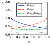
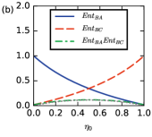
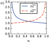
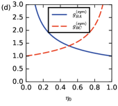
Figure 8: Monogamy of the bipartite PPT entanglement quantifier $Ent$ for the tripartite state of Figure 2, assuming no extra loss or noise. The $Ent_{BA}$, $Ent_{BC}$, $Ent_{BA}Ent_{BC}$ and the monogamy bound $M_{B}$ (gray dotted line) given by equation (43) are plotted versus $\eta_{0}$. In this case, there is steering ($S_{B|\{AC\}}<1$) for all $\eta_{0}$. Here $r=0.5$ (a) and $r=2$ (b). For this system, the symmetry parameters (Fig. (c) and (d)) satisfy $g_{BA}^{(sym)},g_{BC}^{(sym}>1$. Saturation of the monogamy relation (42) is observed for all $\eta_{0}$ for larger $r$ (Fig. (b)), where the gray dotted and green dashed lines coincide.

In Figure 8 we illustrate the monogamy relation with respect to the idealised tripartite system depicted in Figure 2 and Figure 3. For this system there are no additional losses or noise and the covariances are given by Eq. (11). The expression for $Ent_{BA}$ is

$$Ent_{BA}=\frac{n_{BA}-2g_{BA}^{(sym)}c_{BA}+\left(g_{BA}^{(sym)}\right)^{2}m_{BA}}{1+\left(g_{BA}^{(sym)}\right)^{2}}$$ (44)

where $n_{BA},m_{BA}$ and $c_{BA}$ are given by (11). The $Ent_{BC}$ is given similarly, replacing $\eta_{0}$ with $1-\eta_{0}$. It can be verified that the symmetry parameters satisfy $g_{BA}^{(sym)},\ g_{BC}^{(sym}>1$ implying that the monogamy bound $M_{B}$ reduces below $1$. In fact for this case, we find

$$g_{BA}^{(sym)} = \frac{1}{2\sqrt{\eta_{0}}\sinh 2r}\biggl{(}\cosh 2r(1-\eta_{0})-\left(1-\eta_{0}\right)$$

$$+\sqrt{\left(\cosh 2r(1-\eta_{0})-1+\eta_{0}\right)^{2}+4\eta_{0}\sinh^{2}2r}\Biggr{)}$$

and $g_{BC}^{(sym)}$ is obtained by replacing $\eta_{0}$ with $1-\eta_{0}$. These parameters are plotted in Figure 8. We see that $g_{BA}^{(sym)}=g_{BC}^{(sym)}$ for $\eta_{0}=0.5$. The results for the monogamy of entanglement as measured by the quantifier $Ent$ indeed show a greater sensitivity than those for $D$. Where the squeeze parameter $r$ is higher, there is a greater bipartite entanglement created between modes $B$ and $F$ and the collective steering is greater. The higher value of $r$ also indicates a greater degree of genuine tripartite entanglement between the three modes, as measured by inequalities derived in Refs. runyantri ; trivL . We see from the Figure 8(b) that the monogamy relation is saturated for all values of $\eta_{0}$ in the high $r$ regime. This contrasts with the result of Figure 4 for $D$ where the saturation is only at $\eta_{0}=0.5$.

IV.1 Extra loss in the shared mode $B$

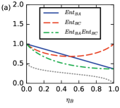
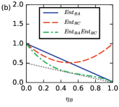
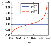
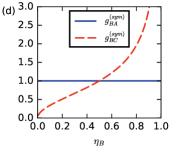
Figure 9: Monogamy for the tripartite state of Figure 2 with equal observed losses for modes $B$ and $A$ ($\eta_{B}=\eta_{0}$). The $Ent_{BA}$, $Ent_{BC}$, $Ent_{BA}Ent_{BC}$ and the monogamy bound $M_{B}$ (gray dotted line) versus $\eta_{B}$. Here $r=0.5$ (a) and $r=2$ (b). In this case, there is steering $S_{B|\{AC\}}<1$ over the whole parameter range. The symmetry parameters satisfy $g_{BA}^{(sym)}=1$ (for all $\eta_{0}$) and $g_{BC}^{(sym)}=1$ only for $\eta_{0}=0.5$.

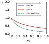
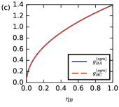
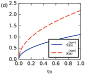
Figure 10: Monogamy for the tripartite state of Figure 2 with extra losses for mode $B$. The $Ent_{BA}$, $Ent_{BC}$, $Ent_{BA}Ent_{BC}$ and the monogamy bound $M_{B}$ (gray dotted line) versus $\eta_{B}$ for $r=2$. Here we take $\eta_{0}=0.5$ (a) and $\eta_{0}=0.8$ (b). Saturation is obtained for the symmetric case of Fig (a) over all $\eta_{B}$ (the gray dotted and green dashed lines coincide).

This case is discussed in the Section III. A, where it was shown that steering exists (such that $S_{B|\{AC\}}<1$) over all values of the attenuated efficiency $\eta_{B}$ for mode $B$. In Figure 9 we plot the entanglement monogamy relations and the symmetry parameters for the case of Figure 4 where the value of loss on mode $B$ matches that of $\eta_{0}$ ($\eta_{B}=\eta_{0}$). This implies symmetry of entanglement between $A$ and $B$ so that $g_{BA}^{(sym)}=1$. As $\eta_{B}$ is varied from $1$ (no loss) to zero (high loss), the symmetry parameter $g_{BC}^{(sym)}$ varies from above to below $1$, being equal to $1$ when $\eta_{b}=\eta_{0}=0.5$ (Figures 9 (c) and (d)). At that point, the monogamy relation for $Ent_{BA}$ and $Ent_{BC}$ is then equivalent to that for $D_{BA}$ and $D_{BC}$, and there is saturation of the monogamy inequality. As $\eta_{B}\rightarrow 1$, $g_{BC}^{(sym)}$ becomes large and the monogamy bound $M_{B}$ becomes small. Indeed the entanglement product is small in this regime. We note however that with $A$ and $B$ sharing excellent symmetric entanglement, the amount of entanglement shared between $B$ and $C$ is reduced and, as seen from the monogamy relation for the symmetric entanglement $D_{BC}$ (Figure 4), is necessarily highly asymmetric.

In Figure 10 we plot the monogamy relation and the symmetry parameters for the situation of Figure 5 where the loss in mode $B$ is varied across all values for fixed $\eta_{0}$. The value of $g_{BA}^{(sym)}$ becomes small when there is considerable loss at the mode $B$, so that $\eta_{B}\ll\eta_{0}$. Similarly, the value of $g_{BC}^{(sym)}$ is small if $\eta_{B}\ll 1-\eta_{0}$. This implies an increased lower bound $M_{B}$ for the monogamy relation. We note from Figure 10 (a) a second regime of saturation of the monogamy relation, where $\eta_{0}=0.5$ and $\eta_{B}$ varies from $0$ to $1$. This regime corresponds to collective steering where $S_{B|\{AC\}}<1$, but we note that (unlike the saturation case of Fig. 8 (b)), the steering parameter is not optimal ($S_{B|\{AC\}}>0$).

IV.2 Extra loss for modes $A$ and $C$

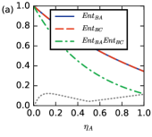
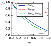
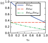
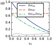
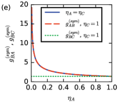
Figure 11: Monogamy for the tripartite state of Figure 2 with extra losses for modes $A$ and $C$. The $Ent_{BA}$, $Ent_{BC}$ and $Ent_{BA}Ent_{BC}$ versus $\eta_{A}$ where $\eta_{B}=1$ for $r=2$. The monogamy bound $M_{B}$ is shown by the gray dotted line. Plots (a) and (b) assume $\eta_{A}=\eta_{C}$ where $\eta_{0}=0.5$ (a) and $\eta_{0}=0.8$ (b). Plots (c) and (d) show values where $\eta_{C}=1$. The steering parameter is given by Figure 6 (e). Plot (e) gives the symmetry parameter $g_{BA}^{(sym)}=g_{BC}^{(sym)}$ for $\eta_{A}=\eta_{C}$ and $g_{BA}^{(sym)}$, $g_{BC}^{(sym)}$ for $\eta_{C}=1$.

To test the relation of Result (2), we need to consider where the steering of $B$ as detected by $S_{B|\{AC\}}<1$ is not possible, so that $S_{B|\{AC\}}>1$. We test the relation by adding losses to the “steering modes”, $A$ and $C$. The covariances are given in the Section III.B. The steering parameter is given by Eq. (30) and can exceed $1$ when $\eta_{F}<0.5$. In Figure 11, we plot the values for the entanglement quantifiers and demonstrate the entanglement monogamy relation. Both the relevant symmetry parameters become large as the extra loss increases ($\eta_{A}$, $\eta_{C}$ becoming small). The steering reduces ($S_{B|\{AC\}}>1$) and overall the monogamy bound $M_{B}$ also becomes small, despite the lack of collective steering (Fig. 6 (e)). We note there is entanglement maintained between both parties ($Ent_{BA}<1$, $Ent_{BC}<1$) over the full parameter range. The entanglement shows high asymmetry however, as indicated by the symmetry parameters plotted in Fig. 11(e) and by the contrasting results for the symmetric entanglement ($D_{BA}$, $D_{BC}$) given in Figure 6.

IV.3 Squeezed thermal two-mode state

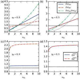
Figure 12: Monogamy relation with thermal noise present: The $Ent_{BA}$, $Ent_{BC}$, $Ent_{BA}Ent_{BC}$ and the monogamy bound $M_{B}$ (dashed line) for $r=1$ for the regime of Figure 7 where $\eta_{B}=1$. Plots give curves for versus thermal noise values where we take $n_{th}=n_{F}=n_{B}$, for (a) $\eta_{0}=0.8$ and (b) $\eta_{0}=0.5$. The monogamy parameter $M_{B}$ is given by the lower gray dotted line. The symmetry parameters are plotted in (c) (for $\eta_{0}=0.8$) and (d) (for $\eta_{0}=0.5$).

As for the Section III.C, we can also test the full monogamy relation by including thermal noise. This is achieved by considering the squeezed thermal two-mode state, as described in Section III. C. In Figure $12$ we plot for various thermal noise values the monogamy product against the lower bound $M_{B}$, allowing for when there is no steering so that $S_{B|\{AC\}}^{2}\geq 1$. We note the values of the symmetry parameters are above $1$, but the steering parameter can also exceed $1$. The overall monogamy bound is plotted in Figure 11 and shows significant increase as the thermal noise increases and the steering indicated by $S_{B|\{AC\}}<1$ is lost. The entanglement product therefore must similarly increase, making entanglement between both parties impossible. This contrasts with the results of Figure 11 where, although the steering is lost, the monogamy bound is low being better balanced by the symmetry parameters. In that case, the entanglement product goes below $1$ and we obtain bipartite entanglement between both pairs.

Conclusion

We have derived monogamy relations for the bipartite entanglement distribution of three systems $A$, $B$ and $C$ modelled as modes. The relations hold for three modes regardless of the tripartite state involved, and may therefore have application to quantum information protocols where two observers $A$ and $B$ have knowledge of the entanglement between them and desire to place a lower bound on the entanglement between one of their parties $B$ and a third observer, Eve, at site $C$.

In Section IV, we present Result (4) where we use as a bipartite entanglement quantifier the Einstein-Podolsky-Rosen variance product involving continuous variable (CV) measurements, that we call $Ent_{AB}$. This quantifier has been shown to give an entanglement condition $Ent_{AB}<1$ equivalent to the Peres-Simon necessary and sufficient condition for highly useful continuous variable Gaussian state resources. Ideal entanglement is achieved when $Ent_{AB}\rightarrow 0$. We show that the lower bound for the entanglement product $Ent_{BA}Ent_{BC}$ depends on the quantum noise level, and also the size of a conventional steering parameter $S_{B|\{AC\}}$ (that for $S_{B|\{AC\}}<1$ certifies a steering of system $B$ from the combined system $A$ and $C$). When there is steering $S_{B|\{AC\}}<1$, the monogamy lower bound is determined by the vacuum quantum noise level. Otherwise, the bound is higher and is constrained by the steering parameter. The lower bound also depends on symmetry parameters $g_{BA}^{(sym)}$ and $g_{BC}^{(sym)}$ which quantify the amount of symmetry between the moments of $B$ and $A$, and $B$ and $C$, respectively. These parameters take the value $g^{(sym)}=1$ when the moments are perfectly symmetrical. In the Section IV, we illustrate the application of this monogamy relation for the tripartite system created using a two-mode squeezed state and a beam splitter. We show that when the two-mode squeezing is high, the monogamy relation is always saturated (reaching the lowest possible monogamy bound). We also study the case of a thermal two-mode squeezed state and where there is extra dissipation.

In Section IV, we also obtain more general monogamy relations (Result (3)) that constrain the shared entanglement as measured by other entanglement certifiers. An example is a relation for the well-known TDGCZ bipartite certifier $D_{BA}$ that gives a necessary and sufficient entanglement condition for symmetric two-mode gaussian states (where $g_{BA}^{(sym)}=1$), which we study in Section II. Although not as sensitive as the more general relation, this can be useful in establishing rigorous bounds on the value of $D_{BA}$ when knowledge of the symmetry parameters is absent, or where only the symmetric form of entanglement is required. We are able to replicate the saturation result of Section IV where the modes have complete symmetry with respect to bipartite moments, hence giving insight into the experiment of Bowen et al.

Appendix

For convenience, in the proofs below we may abbreviate the notation for the variance to denote $(\Delta X)^{2}=\Delta^{2}X$.

Proof of Result 1

First we note that

$$\Delta(X_{B}-X_{A})\geq\Delta(X_{B}|X_{A})$$ (46)

where $(\Delta(X_{B}|X_{A}))^{2}$ denotes the average variance defined as

$$\Delta^{2}(X_{B}|X_{A})=\sum_{x_{A}}P(x_{A})\sum_{x_{B}}P(x_{B}|x_{A})(x_{B}-\mu_{B|x_{A}})^{2}$$ (47)

where $\{x_{A}\}$ is the set of all possible outcomes for $X_{A}$ and denoting $\mu_{B|x_{A}}$ as the mean of $P(X_{B}|X_{A}=x_{A})$. The result (46) is proved as follows: We write

$$\Delta^{2}(X_{B}-X_{A}) = \sum_{x_{B},x_{A}}P(x_{B},x_{A})\left[x_{B}-x_{A}-\langle x_{B}-x_{A}\rangle\right]^{2}$$

$$= \sum_{x_{A}}P(x_{A})\sum_{x_{B}}P(x_{B}|x_{A})(x_{B}-g_{x_{A}})^{2}$$

$$\geq \sum_{x_{A}}P(x_{A})\sum_{x_{B}}P(x_{B}|x_{A})(x_{B}-\mu_{B|x_{A}})^{2}$$

where we introduce $g_{x_{A}}=x_{A}-\langle x_{A}\rangle+\langle x_{B}\rangle$. We have used that for any distribution, $\sum_{x}P(x)(x-g)^{2}$ where $g$ is a constant is minimised by the choice $g=\langle x\rangle=\sum_{x}P(x)x$.

We can introduce the notation $\Delta_{inf}^{2}X_{B|A}=\Delta^{2}(X_{B}|X_{A})$. The notation $\Delta_{inf}^{2}X_{B|A}$ is also often taken to mean the minimum conditional variance average where the measurement $X_{A}$, that we might call $X_{\theta}$, has been chosen optimally to give the best average inference of $X_{B}$. Regardless of the definitions, $\Delta^{2}\left(X_{B}|X_{A}\right)\geqslant\Delta_{inf}^{2}X_{B|A},$ and it follows that $\Delta^{2}(X_{B}-X_{A})\geqslant\Delta_{inf}^{2}X_{B|A}$.

The main proof will now be made by contradiction. Let us consider that $D_{BA}+D_{BC}<1$. Then it follows that:

$$\Delta_{inf}^{2}X_{B|A}+\Delta_{inf}^{2}P_{B|A}+\Delta_{inf}^{2}X_{B|C}+\Delta_{inf}^{2}P_{B|C} < 4$$

We use the identity $2xy\leqslant x^{2}+y^{2},$ to get that $2\Delta_{inf}X_{B|A}\Delta_{inf}P_{B|A}\leqslant\Delta_{inf}^{2}X_{B|A}+\Delta_{inf}^{2}P_{B|A},$ and $2\Delta_{inf}X_{B|C}\Delta_{inf}P_{B|C}\leqslant\Delta_{inf}^{2}X_{B|C}+\Delta_{inf}^{2}P_{B|C}.$ This implies

$$\Delta_{inf}X_{B|A}\Delta_{inf}P_{B|A}+\Delta_{inf}X_{B|C}\Delta_{inf}P_{B|C}<2$$

Next we notice that we can write the above inequality in terms of the steering parameter $S_{B|A}$ which is defined as MR_EPR :

$$S_{B|A}=\Delta_{inf}X_{B|A}\Delta_{inf}P_{B|A}$$ (50)

It follows that $S_{B|A}+S_{B|C}<2,$ and this implies that $S_{B|A}S_{B|C}<1$ (using the identity $2xy\leqslant x^{2}+y^{2}$ again). Thus, $D_{BA}+D_{BC}<1$ implies $S_{B|A}S_{B|C}<1$, which gives a contradiction, since it has been proved in MR_Monogamy2013 that $S_{B|A}S_{B|C}\geq 1$, which is a monogamy inequality for steering. The steering monogamy result was proved valid in Ref. MR_Monogamy2013 for all three mode quantum states. Details of the proof were also given in the Supplementary Materials of Ref. seiji . Thus, by contradiction, we have proved $D_{BA}+D_{BC}\geq 1$ as required.

Proof of Result (2)

Since we have already proved $D_{BA}+D_{BC}\geqslant 1,$ we only require to prove $D_{BA}+D_{BC}\geqslant S_{B|\{AC\}}$. We prove by contradiction. Let us assume that $D_{BA}+D_{BC}<S_{B|\{AC\}}$. In analogy to the proof for (5) we obtain:

$$\Delta_{inf}^{2}X_{B|A}+\Delta_{inf}^{2}P_{B|A}+\Delta_{inf}^{2}X_{B|C}+\Delta_{inf}^{2}P_{B|C}$$

$$<4S_{B|\{AC\}}$$ (51)

Next using the identity $2xy\leqslant x^{2}+y^{2},$ we get that $\Delta_{inf}X_{B|A}\Delta_{inf}P_{B|A}+\Delta_{inf}X_{B|C}\Delta_{inf}P_{B|C}<2S_{B|\{AC\}}$. Using the definition of the steering parameter defined in Eq. (50) we obtain that $S_{B|A}+S_{B|C}<2S_{B|\left\{AC\right\}}$, which gives a contradiction, since it has been proved in MR_Monogamy2013 that $S_{B|A}+S_{B|C}\geqslant 2S_{B|\left\{AC\right\}}$ based on the fact the accuracy to give an inference of $X_{B}$ cannot be decreased if the extra system $C$ is included with $A$, so that $S_{B|A}\geq S_{B|\{AC\}}$.

Proof of Result (3)

Straightforward extension of the proof given in lines (46-LABEL:eq:proof) leads to the following result: By definition, $\Delta^{2}(X_{B}-g_{x}X_{A})=\sum_{x_{B},x_{A}}P(x_{B},x_{A})\left[x_{B}-g_{x}x_{A}-\langle x_{B}-g_{x}x_{A}\rangle\right]^{2}$. Hence we can rewrite

$$\Delta^{2}(X_{B}-g_{x}X_{A}) = \sum_{x_{A}}P(x_{A})\sum_{x_{B}}P(x_{B}|x_{A})(x_{B}-f\left(x_{A}\right))^{2}$$

$$\geq \sum_{x_{A}}P(x_{A})\sum_{x_{B}}P(x_{B}|x_{A})(x_{B}-\mu_{B|x_{A}})^{2}$$

$$= \Delta_{inf}^{2}X_{B|A}$$

where $f\left(x_{A}\right)=g_{x}x_{A}+\langle x_{B}\rangle-g_{x}\langle x_{A}\rangle$. Here, $f\left(x_{A}\right)$ minimises the expression when $f\left(x_{A}\right)=\sum_{x_{B}}P(x_{B}|x_{A})x_{B}=\mu_{B|x_{A}}$. This is true for any real constant $g_{x}$. Thus

$$\Delta^{2}(X_{B}-g_{x}X_{A})\geqslant\Delta_{inf}^{2}X_{B|A}$$ (52)

and similarly $\Delta^{2}(P_{B}-g_{p}P_{A})\geqslant\Delta_{inf}^{2}P_{B|A}$ where $g_{x}$, $g_{p}$ are any real constants. Using the definition given in Eq. (39) and with similar identities for $Ent_{BC}$, we obtain:

$$Ent_{BA}Ent_{BC}$$

$$\geqslant\frac{\Delta_{inf}X_{B|A}\Delta_{inf}P_{B|A}}{1+g_{BA}^{2}}\frac{\Delta_{inf}X_{B|C}\Delta_{inf}P_{B|C}}{1+g_{BC}^{2}}$$

$$=\frac{S_{B|A}S_{B|C}}{\left(1+g_{BA}^{2}\right)\left(1+g_{BC}^{2}\right)}$$

$$\geq\frac{1}{\left(1+g_{BA}^{2}\right)\left(1+g_{BC}^{2}\right)}$$ (53)

as required. Here we have used the steering monogamy inequality $S_{B|A}S_{B|C}\geq 1$ of Ref.MR_Monogamy2013 .

We next prove the second inequality. Since $S_{B|\left\{AC\right\}}\leqslant S_{B|A}$ and $S_{B|\left\{AC\right\}}\leqslant S_{B|C}$, we can write the following identities:

$$Ent_{BA}\geqslant\frac{\Delta_{inf}X_{B|A}\Delta_{inf}P_{B|A}}{1+g_{BA}^{2}}=\frac{S_{B|A}}{1+g_{BA}^{2}}\geqslant\frac{S_{B|\left\{AC\right\}}}{1+g_{BA}^{2}}$$ (54)

with a similar relation for $Ent_{B|C}$:

$$Ent_{BC}\geqslant\frac{S_{B|\left\{AC\right\}}}{1+g_{BC}^{2}}$$ (55)

From the inequalities given in Eq. (54) and Eq. (55), we can derive the following monogamy relations:

$$Ent_{BA}+Ent_{BC}\geqslant S_{B|\{AC\}}\left(\frac{1}{1+g_{BA}^{2}}+\frac{1}{1+g_{BC}^{2}}\right)$$ (56)

and

$$Ent_{BA}Ent_{BC}\geqslant\frac{S_{B|\left\{AC\right\}}^{2}}{\left(1+g_{BA}^{2}\right)\left(1+g_{BC}^{2}\right)}$$ (57)

Outline of proof of steering monogamy inequality

Here, we outline the derivation of the steering monogamy result

$$S_{A|C}S_{A|B}\geq 1$$ (58)

where $S_{A|B}=\Delta_{inf}X_{A|B}\Delta_{inf}P_{A|B}$ that has been used in the above proofs. The monogamy result is proven in Ref. MR_Monogamy2013 , but for the sake of completeness is given here in the more detailed form previously presented in the Supplementary Materials of Ref. seiji . The average conditional “inference” variances are defined in Section II as:

$$[\Delta_{inf}X_{A|B}]^{2}=\sum_{x_{B}}P(x{}_{B})[\Delta(X_{A}|x{}_{B})]^{2}$$ (59)

and

$$[\Delta_{inf}P_{A|B}]^{2}=\sum_{p_{B}}P(p{}_{B})[\Delta(P_{A}|p{}_{B})]^{2}$$ (60)

where $x_{B}$ ($p_{B}$) are the possible results of a measurement performed on system $B$ and on comparing with the Eq. (9) we see that $[\Delta(X_{A}|x_{B})]^{2}=\sum_{x_{A}}P(x_{A}|x_{B})(x_{A}-\mu_{A|x_{B}})^{2}$ and similarly for $\Delta(P_{A}|p_{B})$. The best choice of measurement for $x_{B}$ is that which optimizes the inference of $X_{A}$ though this is not essential to the validity of the monogamy result. Similarly, $p_{B}$ are the possible results for a second measurement performed at $B$, usually chosen to optimize the inference of $P_{A}$.

To derive the relation, we note that the observer (Bob) at $B$ can make a local measurement $O_{B}$ to infer a result for an outcome of $X_{A}$ at $A$. The set of values denoted by $x_{B}$ are the results for the measurement $O_{B}$, and $P(x_{B})$ is the probability for the outcome $x_{B}$. The conditional distribution $P(X_{A}|x_{B})$ has a variance which we denote by $[\Delta(X_{A}|x{}_{B})]^{2}$. The $(\Delta_{inf}X_{A|B})^{2}$ is thus the average conditional variance. Similarly, the observer can make another measurement, denoted $Q_{B}$, to infer a result for the outcome of $P_{A}$ at $A$. Denoting the results of this measurement by the set $p_{B}$, we define the conditional variances as for $X_{A}$.

A third observer $C$ (“Charlie”) can also make such inference measurements, with uncertainty $\Delta_{inf}X_{B|C}$ and $\Delta_{inf}P_{B|C}$. Let us denote the outcomes of Charlie’s measurements, for inferring Alice’s $X_{A}$ or $P_{A}$, by $x_{C}$ and $p_{C}$ respectively. Since Bob and Charlie can make the measurements simultaneously, a conditional quantum density operator $\rho_{A|\{x_{B},p_{C}\}}$ for system $A$, given the outcomes $x_{B}$ and $p_{C}$ for Bob and Charlie’s measurements, can be defined. The $P(x_{B},p_{C})$ is the joint probability for these outcomes. The moments predicted by this conditional quantum state must satisfy the Heisenberg uncertainty relation. That is, we can define the variance of $X_{A}$ conditional on the joint measurements as $\Delta(X_{A}|x{}_{B},p_{C})$ and $\Delta(P_{A}|x{}_{B},p_{C})$ and these must satisfy $\Delta(X_{A}|x{}_{B},p_{C})\Delta(P_{A}|x_{B},p_{C})\geq 1$. We also note that $[\Delta_{inf}X_{A|B}]^{2}\geq\sum_{x_{B},p_{C}}P(x_{B},p_{C})[\Delta(X_{A}|x{}_{B},p_{C})]^{2}$ and $[\Delta_{inf}P_{A|C}]^{2}\geq\sum_{x_{B},p_{C}}P(x_{B},p_{C})[\Delta(P_{A}|x{}_{B},p_{C})]^{2}$ (proved in the Result L below). We see that

$$[\Delta_{inf}X_{A|B}\Delta_{inf}P_{A|C}]^{2} = \sum_{x_{B},p_{c}}P(x_{B},p_{C})[\Delta(X_{A}|x{}_{B},p_{C})]^{2}$$

$$\times\sum_{x_{B},p_{c}}P(x_{B},p_{C})[\Delta(P_{A}|x{}_{B},p_{C})]^{2}$$

Then using the Cauchy-Schwarz inequality and taking the square root, we obtain

$$\Delta_{inf}X_{A|B}\Delta_{inf}P_{A|C} = \sum_{x_{B},p_{C}}P(x_{B},p_{C})$$ (62)

$$\times\Bigl{(}\Delta(X_{A}|x{}_{B},p_{C})\Delta(P_{A}|x_{B},p_{C})\Bigr{)}$$

$$\geq 1$$

Similarly, Bob can measure to infer $P_{A}$ and Charlie can measure to infer $X_{A}$, and it must also be true that

$$\Delta_{inf}P_{A|B}\Delta_{inf}X_{A|C}\geq 1.$$ (63)

Hence, it must be true that $S_{A|B}S_{A|C}\geq 1$.

Result L: Step by step we show the following:

$$[\Delta(X_{A}|x_{B})]^{2} = \sum_{X_{A}}P(X_{A}|x_{B})(X_{A}-\mu_{x_{B}})^{2}$$

$$= \frac{1}{P(x_{B})}\sum_{X_{A}}P(X_{A},x_{B})(X_{A}-\mu_{x_{B}})^{2}$$

$$= \frac{1}{P(x_{B})}\sum_{X_{A}}\sum_{p_{C}}P(X_{A},x_{B},p_{C})(X_{A}-\mu_{x_{B}})^{2}$$

$$\geq \frac{1}{P(x_{B})}\sum_{p_{C}}p(x_{B},p_{C})$$

$$\times\sum_{X_{A}}P(X_{A}|x_{B},p_{C})(X_{A}-\mu_{x_{B},p_{C}})^{2}$$

$$= \frac{1}{P(x_{B})}\sum_{p_{C}}p(x_{B},p_{C})[\Delta(X_{A}|x_{B},p_{C})]^{2}$$

Here $\mu_{x_{B}}$is the mean of $P(X_{A}|x_{B})$ and $\mu_{x_{B},p_{C}}$ is the mean of $P(X_{A}|x_{B},p_{C})$. We note that the value of the constant $\mu$ that minimizes $\langle(x-\mu)^{2}\rangle$ will be the mean of the associated probability distribution. $\square$ In many papers, and in the calculations given in Sections III of this paper, the values for the inference variances as defined in (59-60) are determined by linear optimization. It is explained in Ref. rrmp that the value determined this way cannot be less than the (smallest) value given by the definition (59-60). Furthermore, for Gaussian states, the values according to the two definitions become equal.

References

- (1) V. Coffman, J. Kundu and W. K. Wootters, Distributed entanglement, Phys. Rev. A 61, 052306 (2000).
- (2) T. J. Osborne and F. Verstraete, General monogamy inequality for bipartite qubit entanglement, Phys. Rev. Lett. 96, 220503 (2006).
- (3) Y.-C. Ou, H. Fan, and S.-M. Fei, Proper monogamy inequality for arbitrary pure quantum states, Phys. Rev. A 78, 012311 (2008).
- (4) G. Adesso and F. Illuminati, Continuous variable tangle, monogamy inequality, and entanglement sharing in Gaussian states of continuous variable systems. New J. Phys. 8 15 (2006); T. Hiroshima, G. Adesso and F. Illuminati, Monogamy Inequality for Distributed Gaussian Entanglement, Phys. Rev. Lett. 98, 050503 (2007); G. Adesso and F. Illuminati, Strong Monogamy of Bipartite and Genuine Multipartite Entanglement: The Gaussian Case, Phys. Rev. Lett. 99, 150501 (2007).
- (5) G. Adesso, A. Serafini, and F. Illuminati, Multipartite entanglement in three-mode gaussian states of continuous-variable systems: Quantification, sharing structure, and decoherence, Phys. Rev. A 73, 032345 (2006).
- (6) G. Adesso, D. Girolami and A. Serafini, Measuring Gaussian Quantum Information and Correlations Using the Rényi Entropy of Order 2. Phys. Rev. Lett. 109, 190502 (2012).
- (7) Y.-K. Bai, Y.-F. Xu and Z. D. Wang, General Monogamy Relation for the Entanglement of Formation in Multiqubit Systems, Phys. Rev. Lett. 113, 100503 (2014).
- (8) Y.-K. Bai, N. Zhang, M.-Y. Ye and Z. D. Wang, Exploring multipartite quantum correlations with the square of quantum discord, Phys. Rev. A 88, 012123 (2013).
- (9) X.-N. Zhu and S.-M. Fei, Entanglement monogamy relations of qubit systems, Phys. Rev. A 90, 024304 (2014).
- (10) B. Regula, S. Di Martino, S. Lee and G. Adesso, Strong Monogamy Conjecture for Multiqubit Entanglement: The Four-Qubit Case, Phys. Rev. Lett. 113, 110501 (2014).
- (11) J. Barrett, N. Linden, S. Massar, S. Pironio, S. Popescu, and D. Roberts, Nonlocal correlations as an information-theoretic resource, Phys. Rev. A 71, 022101 (2005). Ll. Masanes, A. Acin, and N. Gisin, General properties of nonsignaling theories, Phys. Rev. A 73, 012112 (2006).
- (12) B. Toner, Monogamy of non-local quantum correlations, Proc. R. Soc. A 465, 59 (2009); B. Toner and F. Verstraete, Monogamy of Bell correlations and Tsirelson’s bound, arXiv:quant-ph/0611001.
- (13) M. D. Reid, Monogamy inequalities for the Einstein-Podolsky-Rosen paradox and quantum steering, Phys. Rev. A 88, 062108 (2013).
- (14) Y. Xiang, I. Kogias, G. Adesso, and Q. Y. He, Multipartite Gaussian steering: monogamy constraints and cryptographical applications, arXiv:1603.08173v1.
- (15) S. Cheng, A. Milne, M. J. W. Hall, and H. M. Wiseman, Volume monogamy of quantum steering ellipsoids for multiqubit systems, Phys. Rev. A 94, 042105 (2016) A. Milne, S. Jevtic, D. Jennings, H. Wiseman, and T. Rudolph, Quantum steering ellipsoids, extremal physical states and monogamy, New J. Phys. 16, 083017 (2014). A. Milne, S. Jevtic, D. Jennings, H. Wiseman, and T. Rudolph, Corrigendum: Quantum steering ellipsoids, extremal physical states and monogamy (2014 New J. Phys. 16 083017), New J. Phys. 17, 019501 (2015).
- (16) G. Adesso and F. Illuminati, Entanglement in continuous-variable systems: recent advances and current perspectives, J. Phys. A: Math. Theor. 40, 7821 (2007). C. Weedbrook, S. Pirandola, R. García-Patrón, N. J. Cerf, T. C. Ralph, J. H. Shapiro, and S. Lloyd, Gaussian quantum information, Rev. Mod. Phys. 84, 621 (2012).
- (17) H. M. Wiseman, S. J. Jones, and A. C. Doherty, Steering, entanglement, nonlocality, and the Einstein-Podolsky-Rosen paradox, Phys. Rev. Lett. 98, 140402 (2007).
- (18) S. J. Jones, H. M. Wiseman, and A. C. Doherty, Entanglement, Einstein-Podolsky-Rosen correlations, Bell nonlocality, and steering, Phys. Rev. A 76, 052116 (2007).
- (19) E. G. Cavalcanti, S. J. Jones, H. M. Wiseman, and M. D. Reid, Experimental criteria for steering and the Einstein-Podolsky-Rosen paradox, Phys. Rev. A 80, 032112 (2009).
- (20) A. Einstein, B. Podolsky and N. Rosen, Can quantum-mechanical description of physical reality be considered complete?, Phys. Rev. 47, 777 (1935).
- (21) M. D. Reid, Demonstration of the Einstein-Podolsky-Rosen paradox using nondegenerate parametric amplification, Phys. Rev. A 40, 913 (1989).
- (22) M. D. Reid, P. D. Drummond, W. P. Bowen, E. G. Cavalcanti, P. K. Lam, H. A. Bachor, U. L. Andersen, and G. Leuchs, Colloquium: The Einstein-Podolsky-Rosen paradox: From concepts to applications, Rev. Mod. Phys. 81, 1727 (2009).
- (23) S. M. Tan, Confirming entanglement in continuous variable quantum teleportation, Phys. Rev. A 60, 2752 (1999).
- (24) L. M. Duan, G. Giedke, J. I. Cirac and P. Zoller, Inseparability Criterion for Continuous Variable Systems, Phys. Rev. Lett. 84, 2722 (2000).
- (25) W. Bowen, R. Schnabel, P. K. Lam, and T. C. Ralph, Experimental investigation of criteria for continuous variable entanglement, Phys. Rev. Lett. 90, 043601 (2003).
- (26) V. Giovannetti, S. Mancini, D. Vitali, and P. Tombesi, Characterizing the entanglement of bipartite quantum systems, Phys. Rev. A 67, 022320 (2003).
- (27) Q. Y. He, Q. H. Gong, and M. D. Reid, Classifying directional Gaussian entanglement, Einstein-Podolsky-Rosen steering, and discord, Phys. Rev. Lett. 114, 060402 (2015).
- (28) Q. Y. He, L. Rosales-Zárate, G. Adesso, and M. D. Reid, Secure continuous variable teleportation and Einstein-Podolsky-Rosen steering, Phys. Rev. Lett. 115, 180502 (2015).
- (29) R. Simon, Peres-Horodecki separability criterion for continuous variable systems, Phys. Rev. Lett. 84, 2726 (2000).
- (30) P. van Loock and A. Furusawa, Detecting genuine multipartite continuous-variable entanglement, Phys. Rev. A 67, 052315 (2003).
- (31) T. Aoki, N. Takei, H. Yonezawa, K. Wakui, T. Hiraoka, A. Furusawa, and P. van Loock, Experimental creation of a fully inseparable tripartite continuous-variable state, Phys. Rev. Lett. 91, 080404 (2003). A. S. Villar, M. Martinelli, C. Fabre, and P. Nussenzveig, Direct production of tripartite pump-signal-idler entanglement in the above-threshold optical parametric oscillator, Phys. Rev. Lett. 97, 140504 (2006).
- (32) A. S. Coelho, F. A. S. Barbosa, K. N. Cassemiro, A. S. Villar, M. Martinelli, and P. Nussenzveig, Three-color entanglement, Science 326, 823 (2009).
- (33) L. K. Shalm, D. R. Hamel, Z. Yan, C. Simon, K. J. Resch, and T. Jennewein, Three-photon energy-time entanglement, Nature Phys. 9, 19 (2013).
- (34) R. Teh and M. D. Reid, Criteria for continuous variable genuine multipartite entanglement and Einstein-Podolsky-Rosen steering, Phys. Rev. A 90 062337 (2014).
- (35) S. Armstrong, J. F. Morizur, J. Janousek, B. Hage, N. Treps, P. K. Lam, and H. A. Bachor, Programmable multimode quantum networks, Nature Commun. 3, 1026 (2012).
- (36) S. Armstrong, M. Wang, R. Y. Teh, Q. Gong, Q. He, J. Janousek, H. Bachor, M. D. Reid and P. K. Lam, Multipartite steering and genuine tripartite entanglement using optical networks, Nature Physics 11, 167 (2015).
- (37) M. D. Reid and P. D. Drummond, Quantum correlations of phase in nondegenerate parametric oscillation, Phys. Rev. Lett. 60, 2731 (1988).
- (38) Q. Y. He and M. D. Reid, Genuine multipartite Einstein-Podolsky-Rosen steering, Phys. Rev. Lett. 111, 250403 (2013).
- (39) B. Yurke and D. Stoler, Generating quantum mechanical superpositions of macroscopically distinguishable states via amplitude dispersion, Phys. Rev. Lett. 57, 13 (1986).
- (40) Q. Y. He and M. D. Reid, Einstein-Podolsky-Rosen paradox and quantum steering in pulsed optomechanics, Phys. Rev. A 88, 052121 (2013).
- (41) L. Rosales-Zárate, R.Y. Teh, S. Kiesewetter, A. Brolis, K. Ng and M. D.Reid, Decoherence of Einstein-Podolsky-Rosen steering, JOSA B 32 A82 (2015).
- (42) S. L. W. Midgley, A. J. Ferris, and M. K. Olsen, Asymmetric Gaussian steering: When Alice and Bob disagree, Phys. Rev. A 81, 022101 (2010). V. Händchen, T. Eberle, S. Steinlechner, A. Samblowski, T. Franz, R. F. Werner, and R. Schnabel, Observation of one-way Einstein–Podolsky–Rosen steering, Nature Photon. 6, 596 (2012).
- (43) I. Kogias, A. R. Lee, S. Ragy and G. Adesso, Gaussian Steering, Phys. Rev. Lett. 114, 060403 (2015).
- (44) P. Marian, T. A. Marian, and H. Scutaru, Bures distance as a measure of entanglement for two-mode squeezed thermal states, Phys. Rev. A 68 062309 (2003).
- (45) B. Opanchuk, Q. Y. He, M. D. Reid, and P. D. Drummond, Dynamical preparation of Einstein-Podolsky-Rosen entanglement in two-well Bose-Einstein condensates, Phys. Rev. A 86, 023625 (2012). S. Kiesewetter, Q. Y. He, P. D. Drummond, and M. D. Reid, Scalable quantum simulation of pulsed entanglement and Einstein-Podolsky-Rosen steering in optomechanics, Phys. Rev. A 90, 043805 (2014).