Using Collisions of AGN Outflows with ICM Shocks as Dynamical Probes

Abstract

In this paper we lay out a simple set of relationships connecting the dynamics of fast plasma jets to the dynamical state of their ambient media. The objective is to provide a tool kit that can be used to connect the morphologies of radio AGNs in galaxy clusters to the dynamical state of the local ICM. The formalism is intended to apply to jets whether they are relativistic or non-relativistic. Special attention is paid to interactions involving ICM shocks, although the results can be applied more broadly. Our formalism emphasizes the importance of the relative Mach number of the impacting ICM flow and the internal Mach number of the AGN jet in determing how the AGN outflows evolve.

I Introduction

Clusters of galaxies are the last and most massive class of bound structures to form out of the Big Bang ($z\raise 1.29167pt\hbox{$<$}\kern-7.5pt{\lower 2.79857pt\hbox{$\sim$}}1,R\sim\rm{Mpc},~{}M\sim 10^{14}-10^{15}\rm{M}_{\odot}$). Cluster assembly combines irregular accretion from surrounding diffuse matter, especially from filaments, and violent mergers with other clusters. As in the universe at large, most cluster matter is non-baryonic, “dark matter”. The baryonic matter within clusters is predominantly hot, diffuse plasma ($kT~{}\raise 1.29167pt\hbox{$>$}\kern-7.5pt{\lower 2.79857pt\hbox{$\sim$}}~{}keV,n_{e}~{}\raise 1.29167pt\hbox{$<$}\kern-7.5pt{\lower 2.79857pt\hbox{$\sim$}}~{}10^{-2}\rm{cm}^{-3}$); the intracluster medium (ICM). The ICMs are shocked and stirred throughout their formation krav12 ; vazz16 ; zing16 . The resulting ICM flow structures provide vital information about the large scale dynamics of cluster formation, as well as about the physics of the ICM plasmaschek06 . Cluster-scale shocks, in particular, are tell-tale consequences of merger events mark07 . Tracing and deciphering these ICM flow structures are essential to our understanding of cluster formation.

While thermal X-rays have successfully revealed some ICM shocks and other flow features mark07 ; walker ; hitomi , distinct X-ray signatures are often subtle and hard to isolate and measure cleanly. Observations of the Sunyaev-Zeldovich effect add some statistical information about the ICM pressure and velocity distributionsadam15 . But, a full, clear picture requires additional, complementary tools. Thankfully, non-thermal synchrotron emissions from $>$ GeV electrons (CRe) in the ICM and in embedded objects may help reach this goal.

So far, the principal non-X-ray tool in efforts to characterize ICM dynamics has been cluster-scale, diffuse radio emissions (radio “halos”, “mini-halos” and “relics”) by electrons within the ICM that are energized or re-energized by cluster shocks and/or turbulence bj14 . There are multiple plausible origins for those diffuse CRe, which in various models may be recent or ancient pinzk15 ; kr15 . Their links to local, current ICM dynamics result from the fact that they have rather short lifetimes against synchrotron losses and inverse Compton scattering of CMB photons ($<$ 100 Myr). Observed CRe must be “energetically younger” than this. Since ICM flow velocities are characteristically $\sim 1$ kpc/Myr, such embedded CRe must have been energized relatively close by on cluster scales. Although these emissions place essential constraints on ICM physics, their translation into distinct and firm ICM dynamical properties has so far proven to be quite challenging kr15 ; don16 .

At the same time, radio-bright, bipolar plasma outflows from active galactic nuclei (radio AGN, henceforth, simply AGN) are common in clusters ledlow96 ; mala16 . Interactions between those outflows and ICM dynamical structures on scales of 10s to 100s of kpc offer an additional and potentially very useful diagnostic probe of the ICM dynamics and physics. That is quite separate from the increasing evidence that AGN-ICM feedback loops on those scales in the cores of relatively undisturbed clusters are central to the properties of those ICMs li15 . The focus of our discussion here, instead, is the consequences of AGN outflow encounters with cluster scale ICM flow structures (especially shocks), and, in particular, impact on the consequent dynamical form of the AGN structures that develop as the AGN plasma penetrates and generate cavities in the ICM.

Specifically, we explore major distortions to the AGN flows and the potential for using such distortions to identify and characterize ICM flow structures, including shocks. In subsequent publications we will present analyses of high resolution 3D MHD simulations of AGN outflows in related dynamical ICM situations. There we will examine details such as coherence and disruption of the AGN flows, development of turbulence, magnetic field evolution, as well as relativistic electron propagation, acceleration and emissions. Our purpose now is more restricted; namely it is to outline a simple, but coherent formalism that we have found to be useful in predicting behaviors of the above simulation experiments and that hopefully captures essential physics needed to interpret observed AGN interactions with dynamical ICMs. We note, in the context of the HEDLA workshop that inspired this work, that many of the dynamical components laid out below should be testable in laboratory experiments.

The best known and most widely discussed AGN distortion produced by asymmetric ICM interactions are those that have formed tails as a result of relative motions between the AGN host galaxy and the surrounding ICM. So-called “Narrow Angle Tailed” (NAT) AGNs, in which the originally collimated AGN outflows appear deflected into a pair of quasi-parallel trails in the wake of the galaxy are especially common in disturbed clusters, where relatively high velocity ICM motions are likely rw68 . If there are apparent, but less dramatic deflections, the AGNs are typically called “Wide Angle Tailed” (WAT) AGNs or76 . Both are obvious candidates as probes of ICM dynamics brb79 ; bliton98 ; sak00 ; mguda15 . The idea that ICM shocks encountering plasma bubbles or cavities left behind by expired AGN might rejuvenate their CRe populations has also been widely discussed eb02 ; pj11 . To the best of our knowledge, however, expected behaviors of active AGN outflows colliding with ICM shocks has not been previously outlined, although there have been several recent suggestions that observed NAT AGN may, in fact, be associated with cluster radio relics bona14 . Here we do not address that issue directly, but do outline the essentials of dynamical encounters of that kind, in order to facilitate future discussions.

Basics of the formalism we outline have been in the literature for some time. Our objective is to set them down as a package, extending them as needed for application to the issues at hand, while looking for parameterizations that may be useful for diagnostic purposes. We specifically target AGN outflow/shock encounters, although the necessary formalism has broader applications. We also include along the way some preliminary results from simulations in order to illustrate the kinds of behaviors that result. We ignore here a number of complications that will ultimately be important to detailed models, but that do not seem essential to a “first order” picture.

Although our goal in this paper is to set out a simple set of analytic relationships, we do show illustrations of behaviors from high resolution numerical simulations that will be discussed in detail in subsequent publications. Those simulations were carried out using the WOMBAT MHD code employing a second order MHDTVD Riemann solver men17 . An adiabatic equation of state with $\gamma=5/3$ was employed. Steady bi-polar jets were formed within a small cylindrical volume, where the jet pressure, $P_{j}$, was kept approximately equal to the ambient pressure, and the jet plasma was accelerated to a velocity, $v_{j}$. All the simulations shown in this paper kept the density within the jet-source cylinder, $\rho_{j}$, at 1% of the undisturbed ambient density. We have, however, varied these parameters to confirm relations described below. We also allowed jet power to cycle off in some cases. The simulated jets were weakly magnetized with a toroidal geometry and nominal $\beta=P_{g}/P_{m}=75$ within the jet-source cylinder. Magnetic stresses are too small to influence dynamics at the levels relevant to this paper. The simulations did include CRe; in follow-up discussions we will discuss in detail synchrotron emission properties. That is beyond the scope of the present paper, however.

The paper outline is this. Section II reviews the interactions between a plane shock and a low density cavity. In section III we outline in simple terms the propagation of a jet into a head or tail wind (section III.1) and into a cross wind (section III.2) that would, for instance, represent post-shock ambient conditions. For completeness section IV sets out a simple model to estimate the form of the plasma cocoon inflated by jets nominally prior to the above interactions.

II An ICM Shock Colliding with a Cavity

Typically the initial encounter between an ICM shock and an AGN will involve the shock penetrating the AGN cocoon/cavity inflated by the AGN outflow. The basic dynamics of such an encounter are qualitatively simple: the core of the cavity is crushed relatively quickly, while the perimeters of the cavity roll into a vortex ring structure eb02 . Here we simply outline of the physics.

Consider then a planar ICM shock of Mach number, $\mathcal{M}_{i}=v_{si}/a_{i}$, where $v_{si}$ is the speed of the shock in the ICM and $a_{i}=\sqrt{\gamma_{i}P_{i}/\rho_{i}}$ is the ICM sound speed. $P_{i}$ and $\rho_{i}$ are the pre-shock ICM pressure and mass density, while $\gamma_{i}$ ($=5/3$) is the ICM adiabatic index. Typical ICM shocks will have modest Mach numbers, $\mathcal{M}_{i}\raise 1.29167pt\hbox{$<$}\kern-7.5pt{\lower 2.79857pt\hbox{$\sim$}}4$, rkhj03 but to allow a wider application of this discussion we do not restrict $\mathcal{M}_{i}$. We then assume the shock encounters a low density cavity, which we take initially to be in pressure equilibrium with the ICM ($P_{c}=P_{i}$). Let the undisturbed density inside the cavity be $\rho_{c}=\delta\rho_{i}$, with $\delta\ll 1$. The initial cavity sound speed is, $a_{c}=\sqrt{\gamma_{c}/\gamma_{i}}~{}a_{i}/\sqrt{\delta}\sim a_{i}/\sqrt{\delta}\gg a_{i}$, where, acknowledging that the cavity includes relativistic plasma, we allow the cavity potentially to have an adiabatic index, $\gamma_{c}\leq\gamma_{i}$, distinct from the ICM.

As the shock encounters the cavity, it penetrates at a speed $v_{sc}=\mathcal{M}_{c}a_{c}\geq a_{c}$ pulling ICM gas with it. Pressure balance between the original cavity and un-shocked ICM leads to the condition, $v_{sc}\geq v_{si}/(\delta^{1/2}\mathcal{M}_{i})$. The original ICM-cavity contact discontinuity (CD) follows the shock at a speed, $v_{cD}$, intermediate between the ICM shock and the cavity shock. At the same time a rarefaction propagates back into the post-shock ICM at the post-shock ICM sound speed.

Pfrommer and Jones pj11 presented the full, nonlinear, 1D Riemann solution to this problem. Here we need only a few, approximate behaviors in order to understand what happens during the encounter. Generally, even though the shock speed is greater inside the cavity, the shock strength is less than the incident shock; that is, $\mathcal{M}_{c}<\mathcal{M}_{i}$. There is no general, analytic formula for $\mathcal{M}_{c}$, although it can be found numerically from the Riemann solution. In the strong shock limit, when $\mathcal{M}_{c}\gg 1$, Pfrommer and Jones found $v_{sc}\sim 2~{}v_{si}$; that is $\mathcal{M}_{c}\sim 2~{}\delta^{1/2}\mathcal{M}_{i}$. In the weak shock limit (as $\mathcal{M}_{c}\rightarrow 1$), of course, $v_{sc}\sim v_{si}\delta^{-1/2}$. In either regime the internal shock speed considerably exceeds the incident, ICM shock speed whenever $\delta\ll 1$. Consequently, the shock passes through the cavity much more quickly than it propagates around it.

The velocity of the CD within the cavity, $v_{CD}$, obtained in the Riemann solution is,

$$v_{CD}=\frac{2}{\gamma_{c}+1}\frac{(\mathcal{M}_{c}^{2}-1)}{\mathcal{M}_{c}^{2}}v_{sc}.$$ (1)

This measures the cavity collapse rate. It will generally be less than $v_{sc}$. However, Pfrommer and Jones found, so long as $\mathcal{M}_{i}\raise 1.29167pt\hbox{$>$}\kern-7.5pt{\lower 2.79857pt\hbox{$\sim$}}2$ and $\delta\ll 1$, that $v_{CD}>v_{si}$. Under those circumstances, the cavity is crushed (the initial CD pushes all the way through the cavity) before the ICM shock propagates around it.

We note that if the cavity has previously developed a thick boundary layer within which $\delta$ is not very small (e.g., through turbulent mixing; see section IV), the internal shock speed within this layer will be slower than above, but $\mathcal{M}_{c}$ can remain comparable to $\mathcal{M}_{i}$ through that boundary layer. This can, for instance, significantly influence such things as particle acceleration during shock passage and shock amplification of turbulence.

If the initial cavity is “round” (e.g., a sphere), the shock intrusion into the cavity begins sooner and is usually stronger at the normal, “point of first contact.” On the other hand, the oblique penetration towards the extremes of the cavity boundary also generates vorticity. An initially spherical cavity will, thus, evolve into a torus, or vortex ring that mixes ICM and cavity plasma eb02 ; pj11 . Analogously, even if the cavity boundary is planar, but the shock normal is oblique to the cavity boundary, refraction of the shock and penetrating CD will produce vorticity and mixing pjr15 . Examples of shocks impacting ICM cavities have been presented previously eb02 ; pj11 . Outcomes are also evident in Figures 2 and 3.

III Jet Propagation in a (Post-shock) Wind

If an AGN jet remains active following shock impact, so that it drives into the post-shock ICM, its propagation will be modified because the post-shock ICM is denser than the pre-shock ICM and also because the post-shock ICM plasma is put in motion by the shock. In this section we outline a toy model to address these effects. The basic geometry is illustrated in Figure 1.

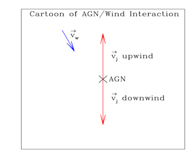
Figure 1: Cartoon illustrating the basic geometry of bipolar AGN jets propagating into an ambient wind.

We approximate the dynamics as that of a jet within an ambient wind, decomposing the wind velocity into components parallel (head wind or tail wind) and orthogonal (cross wind) to the jet velocity vector, $\vec{v_{j}}=v_{j}\hat{v_{j}}$, near its terminus. That is, we set

$$\vec{v}_{w}=v_{w,\parallel}\hat{v}_{j}+v_{w,\perp}\hat{v}_{\perp},$$ (2)

where $\hat{v}_{j}\cdot\hat{v}_{\perp}=0$. When $v_{w,\parallel}\neq 0$; that is, whenever there is a tail wind, $v_{w,\parallel}>0$, or a head wind, $v_{w,\parallel}<0$, the rate of advance of the jet terminus will be modified; when $v_{w,\perp}\neq 0$ the jet propagation will be deflected laterally. Although we present the model in the context of a post-shock flow, the formalism applies to any relative motion between the AGN and its ambient medium. Indeed the model is essentially a merger and modest extension of classical cartoons of AGN jet propagation bbr84 ; brb79 . Simply stated, jet advance and deflection are influenced by parallel and transverse ram pressures created by the wind.

III.1 Advance of a Jet Terminus in an Ambient Head or Tail Wind

We begin by considering the influence of an ambient wind motion aligned with the jet velocity; that is, consequences of $v_{w,\parallel}\neq 0$. To keep the discussion simple we consider here only steady, collimated jets (zero opening angle) and homogeneous ambient media. We adopt the standard picture that the advance of the jet terminus into the ICM can be expressed in terms of the propagation of a contact discontinuity that forms at the head of the jet bbr84 . Relative to the AGN, that boundary (the jet “head”) propagates at velocity, $v_{h}\hat{v}_{j}=d\ell_{j}/dt~{}\hat{v}_{j}$, where $\ell_{j}$ represents the length of the jet from the AGN. There will be a bow shock propagating into the wind, ahead of the head, as well as a reverse, “terminal” shock in the jet. The simple, 1D cartoon model ignores these details, drawing a box around all this and assumes the jet thrust; that is, the total jet momentum flux coming in through an area, $A_{j}=\pi r_{j}^{2}$, is balanced by the total wind momentum flux coming in on the opposite side of the box, again, through an area, $A_{j}$. In reality, because both jet and wind plasma will, as “back flow”, exit the face of the box through which the jet enters (and box sides), the effective sizes of the box faces need to be larger than $A_{j}$. We can crudely account for this asymmetry by setting the effective area allocated to the wind, $A_{h}$, to be larger than the nominal cross section of the jet.

We comment, as well, that even for a collimated jet the radius, $r_{j}$, will not generally be a constant along the length of the jet, especially when it becomes over or under pressured with respect to its surroundings. In that case, for instance, the propagating jet plasma will execute a sequence of expansions and rarefactions around an equilibrium radius. Consequently, the jet velocity, $v_{j}$, density, $\rho_{j}$, and pressure, $P_{j}$, will all vary along a real jet. Our analysis here does not try to account for dynamics at that level of detail, so we will assume below that the jet has some suitably chosen characteristic radius, $r_{j}$, density, $\rho_{j}$ and pressure, $P_{j}$.

We allow both the jet velocity and equation of state (EoS) to be either non-relativistic or relativistic, although we will assume the propagation of the wind and the head through the wind in the AGN reference frame are non-relativistic. Then, the jet 4-velocity is $U_{j}=\Gamma_{j}v_{j}$, with $\Gamma_{j}$ the Lorentz factor of the jet velocity, $v_{j}$, while the enthalpy density of the jet plasma in the jet plasma frame is $w_{j}c^{2}=e_{j}+P_{j}=\rho_{j}c^{2}+e_{j}^{\prime}+P_{j}=\rho_{j}c^{2}\tilde{w}$, with $e_{j}$ the internal energy density of the jet plasma, including rest mass energy, $\rho_{j}c^{2}$. The jet momentum flux density in the AGN frame can be written llfm

$$T_{mj}=w_{j}U_{j}^{2}+P_{j}=\rho_{j}\tilde{w}U_{j}^{2}+P_{j}.$$ (3)

The jet thrust is

$$N_{j}=T_{mj}A_{j}=(w_{j}U_{j}^{2}+P_{j})A_{j}=\rho_{j}U_{j}^{2}(\tilde{w}_{j}+\frac{P_{j}}{\rho_{j}U_{j}^{2}})A_{j}.$$ (4)

For a non-relativistic EoS, where $e\approx\rho c^{2}$, $\tilde{w}=(e+P)/(\rho c^{2})\approx 1+(e^{\prime}+P)/(\rho c^{2})=1+a^{2}/((\gamma-1)c^{2})\approx 1$, while for a relativistic EoS, where $P\approx(1/3)e$, $\tilde{w}\sim 4P/(\rho c^{2})\gg 1$.

It will be useful later on also to have expressions for the jet energy flux density in the AGN frame. Subtracting off the rest mass energy this is

$$T_{ej}=U_{j}\Gamma_{j}(wc^{2}-\rho_{j}c^{2}/\Gamma_{j})$$

$$=U_{j}\Gamma_{j}\rho_{j}c^{2}(\tilde{w}-1/\Gamma_{j})$$

$$=\Gamma_{j}^{2}\rho_{j}c^{2}v_{j}\left[(1-1/\Gamma_{j})+(e_{j}^{\prime}+P_{j})/(\rho_{j}c^{2})\right],$$ (5)

so that the “luminosity” of the jet is

$$L_{j}=T_{ej}A_{j}=v_{j}\Gamma_{j}^{2}\rho_{j}c^{2}(\tilde{w}-1/\Gamma_{j})A_{j}.$$ (6)

We define the internal jet Mach number as, $\mathcal{M}_{j}=\Gamma_{j}v_{j}/(\Gamma_{s,j}a_{j})$,k80 where $a_{j}=c\sqrt{\partial P_{j}/\partial e_{j}}$ is the jet sound speed, with $\Gamma_{s,j}^{2}=1/(1-(a_{j}/c)^{2})$. For a relativistic EoS $a^{2}=(1/3)c^{2}$, while $\Gamma_{s}^{2}=3/2$, so $\Gamma_{s}^{2}a^{2}=(1/2)c^{2}$. Note in this limit that the jet Mach number, $\mathcal{M}_{j}\to\sqrt{2}~{}\Gamma_{j}(v_{j}/c)$, which, if $v_{j}\to c$ gives $\mathcal{M}_{j}=\sqrt{2}~{}\Gamma_{j}$. This makes clear that the fact that a jet velocity is close to the speed of light does not, by itself, imply a high Mach number for the jet dynamics. A non-relativistic EoS with $P=(\gamma-1)e^{\prime}$ recovers the familiar $a^{2}=\gamma P/\rho$.

With these definitions the momentum flux density is

$$T_{mj}=\rho_{j}\tilde{w}\Gamma_{j}^{2}v_{j}^{2}+P_{j}=\mathcal{M}_{j}^{2}P_{j}\left[\frac{a_{j}^{2}}{c^{2}-a_{j}^{2}}\tilde{w}\frac{\rho_{j}c^{2}}{P_{j}}+\frac{1}{\mathcal{M}_{j}^{2}}\right].$$ (7)

Setting $\gamma^{\prime}=(\Gamma_{s,j}^{2}a_{j}^{2}w_{j})/P_{j}$, this becomes simply

$$T_{mj}=\gamma^{\prime}\mathcal{M}_{j}^{2}P_{j}\left[1+\frac{1}{\gamma^{\prime}\mathcal{M}_{j}^{2}}\right].$$ (8)

For a relativistic EoS $\gamma^{\prime}=2$, whereas for a non-relativistic EoS, $\gamma^{\prime}=\gamma$, the usual gas adiabatic index. Written in this form the expression for the jet momentum flux is virtually the same for relativistic or non-relativistic jets. If, as is often the case, $\mathcal{M}_{j}^{2}\gg 1$ we can neglect the second term in square brackets. Then, the jet thrust for either relativistic or non-relativistic flow is

$$N_{j}=T_{mj}A_{j}\approx\gamma^{\prime}\mathcal{M}_{j}^{2}P_{j}A_{j}.$$ (9)

In either regime the thrust depends simply on the internal jet pressure and the internal jet Mach number.

The jet luminosity is not quite so tidy, but still simple to express. For a non-relativistic EoS the luminosity would be

$$L_{j}\approx\mathcal{M}_{j}\Gamma_{j}\rho_{j}c^{2}~{}(\Gamma_{s,j}a_{j})~{}\left[1+\frac{a_{j}^{2}}{(\gamma_{j}-1)c^{2}}-\frac{1}{\Gamma_{j}}\right]A_{j},$$ (10)

which, with $v_{j}\ll c$, but $v_{j}/a_{j}=\mathcal{M}_{j}\gg 1$ and $\gamma_{j}=5/3$ takes the simple familiar form,

$$L_{j}\approx\frac{1}{2}\rho_{j}v_{j}^{3}A_{j}=\frac{5}{6}\mathcal{M}_{j}^{2}v_{j}P_{j}A_{j}.$$ (11)

At the other extreme, with a relativistic EoS, $\tilde{w}_{j}=4P_{j}/(\rho_{j}c^{2})$, and $\Gamma_{j}\gg 1$, the luminosity is also simple to express; namely,

$$L_{j}\approx 2\mathcal{M}_{j}^{2}cP_{j}A_{j},$$ (12)

since, now $2\Gamma_{j}^{2}\approx\mathcal{M}_{j}^{2}$. Again, in this form the relativistic and non-relativistic expressions are almost the same. The jet luminosity can, like the thrust, be described in terms of the jet pressure and Mach number, but now also in terms of a jet speed, $v_{j}$, (which may $\to c$).

We return now to estimating the rate at which the jet terminus propagates through its surrounding plasma. The momentum flux balance condition determining the propagation velocity, $\vec{v}_{h}$, is actually measured in the frame of the head, so we should transform the momentum flux relations to that frame. However, provided $v_{h}/v_{j}\ll(c/v_{j})^{2}/\Gamma_{j}^{2}$, it is easy to show that the fractional change in $T_{mj}$ is small. We will neglect that correction below. The momentum balance condition becomes,

$$N_{j}=A_{j}T_{mj}=A_{h}[\rho_{w}(v_{h}-v_{w,\parallel})^{2}+P_{w}].$$ (13)

Using equation 9 this leads to

$$\frac{(v_{h}-v_{w,\parallel})^{2}}{a_{w}^{2}}\left[1+\frac{a_{w}^{2}}{\gamma_{w}(v_{h}\mp v_{w})^{2}}\right]\approx\mathcal{M}_{j}^{2}\frac{\gamma^{\prime}}{\gamma_{w}}\frac{A_{j}P_{j}}{A_{h}P_{w}}$$ (14)

or,

$$(\mathcal{M}_{h}\mp\mathcal{M}_{w,\parallel})^{2}\left[1+\frac{1}{\gamma_{w}(\mathcal{M}_{h}\mp\mathcal{M}_{w})^{2}}\right]\approx\mathcal{M}_{j}^{2}\frac{\gamma^{\prime}}{\gamma_{w}}\frac{A_{j}}{A_{h}}\frac{P_{j}}{P_{w}}$$ (15)

where $\mathcal{M}_{h}=v_{h}/a_{w}$ and $\mathcal{M}_{w,\parallel}=|v_{w,\parallel}|$ are the Mach numbers of the jet head advance and the head/tail wind with respect to the AGN. Then, of course, $a_{w}=\sqrt{\gamma_{w}P_{w}/\rho_{w}}$ is the wind sound speed. In equations 14 and 15 the upper (lower) sign corresponds to a tail (head) wind.

If $(\mathcal{M}_{h}\mp\mathcal{M}_{w,\parallel})^{2}\gg 1$ we have the simple result

$$|\mathcal{M}_{h}\mp\mathcal{M}_{w,\parallel}|\approx\mathcal{M}_{j}\sqrt{\frac{A_{j}}{A_{h}}}\sqrt{\frac{P_{j}}{P_{w}}}\sqrt{\frac{\gamma^{\prime}}{\gamma_{w}}}.$$ (16)

That is, the Mach number of the advance of the head relative to its ambient medium is similar to the internal Mach number of the jet modified by a factor that depends mostly on the ratio of the integrated jet pressure, $P_{j}A_{j}$, to the integrated wind pressure (isotropic pressure, not ram pressure) “across the head”, $P_{w}A_{h}$. In our simulation experiments with steady, fixed axis, non-relativistic jets $A_{j}/A_{h}\sim 1/2$ provides reasonable matches between simulated jet propagation and equations 14, 15 and 16.

Some insights into appropriate $P_{j}/P_{w}$ are useful going forward. Our discussions relate to jets that are pressure confined as they propagate. So, we expect $P_{j}\sim P_{a}$, where $P_{a}$ represents the pressure of whatever medium is immediately surrounding the jet. If a jet enters a region where it is out of pressure balance, it will generally expand or converge to compensate. As noted above, the pressures within simulated jets are actually quite non-uniform as a result. On average, however, we find, independent of the pressure assignd to a simulated jet at its origin, the average pressure along the propagating jet becomes roughly comparable to the ambient pressure. We also find in simulations and argue in section IV that the pressure inside jet cocoons are commonly roughly similar to those in the undisturbed surroundings, even though the cocoon formation drives a shock into its surroundings. Consequently, we expect within a factor of a few that $P_{j}/P_{w}\sim 1$. Nonetheless, we leave such ratios as undetermined in our analyses, in order to reveal their roles.

We note also for non-relativistic jets with non-relativistic EoS that, since for both the jet and the ambient medium, $a^{2}=\gamma P/\rho$, equation 16 can be written

$$|v_{h}\mp|v_{w,\parallel}||\approx v_{j}\frac{\sqrt{A_{j}/A_{h}}}{\sqrt{\rho_{w}/\rho_{j}}},$$ (17)

independent of $P_{j}/P_{w}$. This recovers the commonly applied assumption that, modulo “an efficiency factor” ($\sqrt{A_{j}/A_{h}}$) the advance speed of the jet head is roughly the jet speed reduced by a factor of the square root of the density ratio between the ambient medium and the jet when the jet and its advance are both highly supersonic bbr84 .

It is further evident from these relations, as we would expect intuitively, that the advance speed of the jet with respect to the AGN, $v_{h}$, is greater when it propagates downstream with a wind (a “tail wind”) than if it propagates upstream into a wind (a “head wind”). In fact a jet propagating into a sufficiently strong head wind can be stopped, or even reversed. Using equation 16 the approximate condition for the head wind to stop forward progress of the head is

$$|\mathcal{M}_{w,\parallel}|\raise 1.29167pt\hbox{$>$}\kern-7.5pt{\lower 2.79857pt\hbox{$\sim$}}\mathcal{M}_{j}\sqrt{\frac{A_{j}}{A_{h}}}\sqrt{\frac{\gamma^{\prime}P_{j}}{\gamma_{w}P_{w}}}.$$ (18)

We have verified this condition in our simulations (see Figure 2).

Although the above results would be applicable for any AGN relative motion through its ambient medium when the AGN jets are aligned with the relative motion, we introduced the issue in the context of post-shock ICM flows. In that case it is useful to express these relations in terms of wind properties resulting from ICM shocks. To keep it simple, we assume that the pre-shock ICM plasma was at rest with respect to the AGN, although that is easily modified. Again expressing the ICM shock Mach number as $\mathcal{M}_{i}$ we have (assuming $\gamma_{w}=\gamma_{i}=5/3$),

$$\rho_{w}=\frac{4\mathcal{M}_{i}^{2}}{\mathcal{M}_{i}^{2}+3}\rho_{i},$$ (19)

$$P_{w}=\frac{5\mathcal{M}_{i}^{2}-1}{4}P_{i},$$ (20)

$$v_{w}=\frac{3}{4}\frac{\mathcal{M}_{i}^{2}-1}{\mathcal{M}_{i}}a_{i},$$ (21)

$$a_{w}^{2}=\frac{(\mathcal{M}_{i}^{2}+3)(5\mathcal{M}_{i}^{2}-1)}{16\mathcal{M}_{i}^{2}}a_{i}^{2}.$$ (22)

where, as above, the subscript index ‘i’ identifies the unshocked ICM, and ‘w’ indicates post-shock ICM (the “wind”).

Applying equations 19 - 22 to equation 18 we obtain an approximate relation for the strength, $\mathcal{M}_{is}$, of an ICM shock that can stop the advance of an approaching jet of internal Mach number, $\mathcal{M}_{j}$ in a “head on collision” when the AGN is at rest in the undisturbed ICM; namely

$$\mathcal{M}_{i}=\mathcal{M}_{i,s}~{}\raise 1.29167pt\hbox{$>$}\kern-7.5pt{\lower 2.79857pt\hbox{$\sim$}}~{}\frac{2}{3}\sqrt{\frac{3\gamma^{\prime}}{5}}\mathcal{M}_{j}\sqrt{\frac{P_{j}}{Pi}}\sqrt{\frac{A_{j}}{A_{i}}}\frac{1}{G(\mathcal{M}_{i})},$$ (23)

where $G(\mathcal{M}_{i})=(1-1/\mathcal{M}_{i}^{2})/\sqrt{1+3/\mathcal{M}_{i}^{2}})\leq 1$. As noted above, we expect for steady jets with fixed axes, $A_{j}/A_{i}\sim 1/2$. The function $G(\mathcal{M}_{i})\sim 0.6-0.9$, for $2\raise 1.29167pt\hbox{$<$}\kern-7.5pt{\lower 2.79857pt\hbox{$\sim$}}\mathcal{M}_{i}\raise 1.29167pt\hbox{$<$}\kern-7.5pt{\lower 2.79857pt\hbox{$\sim$}}4$, corresponding to expected “merger-related” ICM shock strengths. As a rough rule of thumb, then, an AGN jet running head on into a shock will be stopped or reversed if the Mach number of the shock is comparable to or even a bit less than the Mach number of the jet.

The above behaviors are illustrated in Figure 2 for two, simulated non-relativistic shock-jet interactions with different relative shock strengths. The views are 3D volume renderings of jet mass fraction; that is, only plasma that originated from the AGN is shown. In both cases, $\mathcal{M}_{j}=3.5$, and the shock normal was aligned with the (bi-polar) jet axis. ICM shock propagation was left-to-right, although in this view the shock plane was rotated 40 degrees from the line of sight, in order to reveal the structures more clearly. The location of the AGN is marked by an X in each case. The color map of the mass fraction tracer runs from “white” (100%) through yellow, red, green and blue ($\sim$ 30%).

The figure upper panel represents the outcome for an ICM shock with $\mathcal{M}_{i}=2=0.57\mathcal{M}_{j}$, whereas the lower panel involves a $\mathcal{M}_{i}=4=1.1\mathcal{M}_{j}$ shock. Both are shown at approximately the same time interval since initial contact between the shock and the left-facing (upwind) jet. In the bottom panel the stronger shock has left the computational domain to the right after reversing the left-facing jet and crushing the two original jet plasma cocoons and stripping them from the jets. The “smoke ring” to the right is the resulting vortex ring structure, whose formation out of the pre-shock cavities was outlined in the previous section. The flaring seen at the right end of the remaining (downwind) jet represents the head of that jet. The shocked jet plasma is unable to propagate back to the AGN through the strong right-facing wind behind this shock. It is not able to refill a cocoon (see section IV). The jet remains “naked”. Several AGNs in disturbed clusters have been seen that are candidates for this interaction. Probably the best known example is the radio source ‘C’ in A2256, rsm94 ; or14 which has a roughly 1 Mpc, very thin (unresolved) “tail” extending to the west of an AGN, but nothing evident to the east. Indeed, that AGN is seen projected near a strong “radio relic“ in the cluster, suggesting that it could have passed through a moderately strong cluster merger shock.

The weaker and slower ICM shock involved in the upper Figure 2 panel dynamics is still in the volume illustrated, although not directly visible in this rendering. In the undisturbed ICM its position along the jet axis is about 2/3 of the distance from the AGN X to the right end of the right-facing jet head. Inside the right-side cocoon, the shock has just reached the head at this time. We found experimentally in this case that an incident shock with $\mathcal{M}_{i}\approx(3/4)\mathcal{M}_{j}$ would just stop the approaching (left facing in the figure) jet.

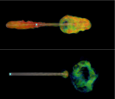
Figure 2: Illustration from simulations of ICM shocks colliding head on with $\mathcal{M}_{j}=3.5$ AGN jet pairs. Both panels are volume renderings of a passive jet mass-fraction tracer. Shock propagation was left to right. ’X’ marks AGN location. The jet axes are rotated 40 degrees out of the plane of the sky with the left jets approaching the observer. Top: $\mathcal{M}i=2$. Bottom: $\mathcal{M}_{i}=4$. See text for details.

Thus, evidence for relative AGN foreshortening to one side has the potential to find and even measure the strengths of ICM shocks or winds.

III.2 Deflection of a Jet by a Cross Wind

In the presence of a cross wind, $v_{w,\perp}\neq 0$ (see Figure 1), the jet is subjected to an unbalanced transverse ram pressure force, $\rho_{w}v_{w,\perp}^{2}$. Particularly, if that cross wind results from a crossing shock, the jet cocoon (cavity) will be crushed and stripped away from the propagating jet (see Figure 3). From that point on the jet interacts directly with the wind, and we can estimate the induced transverse pressure gradient within the jet as

$$\partial P_{j}/\partial x_{\perp}\approx\rho_{w}v_{w,\perp}^{2}/(2r_{j}).$$ (24)

Then the transverse acceleration of a steady jet is determined by the relation

$$\frac{w\Gamma_{j}^{2}v_{j}}{c^{2}}\frac{\partial v_{j,\perp}}{\partial\ell}\approx\frac{\rho_{w}v_{w,\perp}^{2}}{2r_{j}}(1-\Gamma_{j}^{2}v_{j,\perp}^{2}/c^{2}),$$ (25)

We can use $\partial v_{j,\perp}/\partial\ell\sim v_{j}/\ell_{b}$ as a way to estimate the length $\ell_{b}$ over which the transverse ram pressure from the wind will deflect the jet by 90 degrees; that is, the “ jet bending length”. Neglecting the (initially small) second term inside the parentheses in equation 25 this gives,

$$\ell_{b}\approx 2r_{j}\frac{w\Gamma_{j}^{2}v_{j}^{2}}{\rho_{w}v_{w,\perp}^{2}}\approx 2r_{j}\frac{T_{mj}}{\rho_{w}v_{w,\perp}^{2}},$$ (26)

where the final expression has used equation 9. Analogous to the results of the previous subsection we can also write this final form in terms of the jet Mach number, $\mathcal{M}_{j}$ and the cross-wind Mach number, $\mathcal{M}_{w,\perp}$,

$$\ell_{b}\approx 2r_{j}\frac{\gamma^{\prime}}{\gamma_{w}}\frac{\mathcal{M}_{j}^{2}}{\mathcal{M}_{w,\perp}^{2}}\frac{P_{j}}{P_{w}}.$$ (27)

If the jet and wind pressures are comparable, the ratio of the jet bending length, $\ell_{b}$, to the jet diameter, $2r_{j}$, is roughly $(\mathcal{M}_{j}/\mathcal{M}_{w})^{2}$. A little bit of algebra shows that equation 27 matches the bending radius of curvature derived in brb79 for an AGN moving supersonically through an ambient medium at right angles to the jet axis. Of course, only relative motion matters, and here we emphasize that it is not necessary that the cross wind is supersonic for the bending to develop. The bending radius will, however, scale inversely with the square of the Mach number of relative motion. So, once again, obvious distortion in the AGN points to relatively large Mach number of the relative motion between the AGN and its immediate surroundings.

Assuming the cross wind under discussion comes entirely from an ICM shock propagating transverse to the jet axis, we can use equations 19 - 22 to give a relation between the jet bending length, the jet radius, the jet Mach number and the ICM shock Mach number, $\mathcal{M}_{i}$,

$$\ell_{b}\approx\frac{8}{9}\frac{\gamma^{\prime}}{\gamma_{i}}\frac{\mathcal{M}_{j}^{2}(\mathcal{M}_{i}^{2}+3)}{(\mathcal{M}_{i}^{2}-1)^{2}}\frac{P_{j}}{P_{i}}~{}r_{j}.$$ (28)

By convention, when the jet length, $\ell_{j}$ satisfies $\ell_{j}~{}\raise 1.29167pt\hbox{$>$}\kern-7.5pt{\lower 2.79857pt\hbox{$\sim$}}~{}\ell_{b}$, but $\ell_{b}\gg r_{j}$ the resulting AGN morphology would be describe as a “wide angle tail” radio galaxy, or a “WAT”. As the ratio $\ell_{b}/r_{j}$ becomes smaller, the morphological label would shift to “narrow angle tail” or “NAT”.

Figure 3 illustrates results from a simulation of a $\mathcal{M}_{i}=4$ shock that crossed from the left and collided at right angles with a pair of $\mathcal{M}_{j}=10$ jets oriented vertically in the image. Equation 28 predicts $\ell_{b}/r_{j}=6.7$, which is actually very close to the empirical result of the simulation. As in Figure 2 this image shows a volume rendering of the passive jet mass fraction tracer. The shock plane has again been rotated 40 degrees from the line of sight to make 3D structures more distinct. We comment on the close resemblance between the structures visible in Figure 3 and the “classic” NAT source, NGC1265 odea86 , whose morphology has long been modeled in terms of a strong cross wind in the rest frame of the host galaxy. Here the wind is a feature of the post-shock environment. That has also been suggested for NGC1265 pj11 .

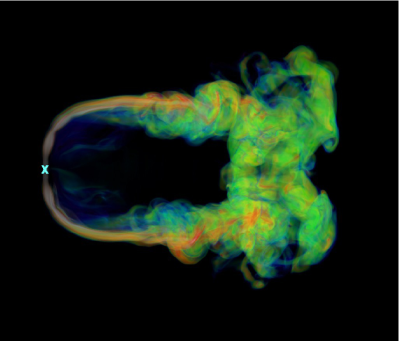
Figure 3: Simulation of an $\mathcal{M}_{i}=4$ shock that crossed from the left and collided at right angles with an $\mathcal{M}_{j}=10$ AGN jet pair (vertical jet axis in the image). Shown is a volume rendering of a passive jet mass-fraction tracer after the shock has passed through the volume shown. ’X’ marks AGN location. View orientation is the same as Figure 2. See text for details.

Note that the two jets in Figure 3 remain stable long after they are deflected by $~{}\sim~{}90$ degrees into “tails”, even though turbulent mixing regions develop around them and enlarge downstream. The tails merge at the far right into a pair of merging vortex rings that formed along the lines outlined in section II as the ICM shock crushed the two jet cocoons produced before shock impact. The jets can be traced as coherent structures almost to the vortex rings. The shock itself has left the observed volume to the right at the time shown.

Finally, we comment on the more complex case where an incident shock collides at an arbitrary angle with respect to the AGN jet axis, or more generally when the AGN jets encounter an oblique wind. Since $v_{w,\perp}$ is initially the same for both jets, the rate of jet deflection indicated by equation 25 would, before deformation, be the same for both jets (see Figure 1).

The aligned wind velocity, $v_{w,\parallel}$, has the same magnitude, but opposite sign on the two jets. The downwind jet, where $v_{w,\parallel}>0$, thus advances more rapidly. As the jets begin to be deflected, however, the upwind jet, where $v_{w,\parallel}<0$, is deflected to be more nearly transverse to the wind ($v_{w,\perp}$ increases along the jet on that side), while the downwind jet is deflected to be more nearly aligned with the wind ($v_{w,\parallel}$ increases along this jet). Consequently, the upwind jet becomes more sharply bent than the downwind jet. We have confirmed in simulations a regular transitioun along these lines between the aligned wind interactions described in section III.1. and cross wind interactions outlined at the beginning of this section. Evidently, such asymmetries can provide information about both the relative Mach numbers of the jets and a wind and the relative orientations of the wind and the jets. The shape evolution of the two jets depends distinctively on the ratio of two Mach numbers as well as the orientation between the AGN jet axis and the wind velocity vector, $\vec{v}w$. Thus, the resulting shape provides a means to determine both $\mathcal{M}_{j}/\mathcal{M}_{w}$ and $\hat{v}_{w}\cdot\hat{v}_{j}$. Also, it is obvious that if the “weather conditions” encountered by jets vary as they extend through the ICM, additional morphological features are likely to develop that can be used to identify and characterize these ICM structures.

IV Formation of a Backflow Cocoon

We began this discussion with an outline of shock propagation through a pre-existing cavity formed by AGN outflows; that is a jet cocoon. Then we outlined propagation of the jets themselves in the post-shock flow. The shocks both crush the cocoon and may, if the wind “stripping” is faster than replacement from the jet terminus, remove the cocoon (see Figures 2 and 3). We did not, however, address what might be learned from the cocoons themselves, In order to tie the pieces together, here we outline briefly some of the related physics connecting the jet propagation to the formation of the jet cocoon before shock impact. Since our purpose is only to lay out a rough picture of cocoon inflation, we ignore in this section complications such as relative motions between the AGN and its ambient ICM, the presence of large scale pressure or density gradients, or ICM turbulence. All of these will modify cocoon morphology and quantitative measures, although they should not fundamentally change the basic picture presented here.

In simple terms the cocoon represents the reservoir of plasma that has previously passed through the jet. The cocoon plasma will generally be of substantially lower density than the surrounding ICM, with the two media nominally separated by a contact discontinuity. Because it is also a “slip surface”, that boundary is likely to be unstable to Kelvin-Helmholtz instabilities (KHI), so that some degree of mixing will take place (unless, for instance, magnetic fields in or around the cocoon are strong enough and coherent enough to stabilize the contact discontinuity rebhp07 ; odj09 ).

Figure 4 shows volume renderings of cocoons formed from two simulated steady AGN jet pairs. In each case the AGN (marked by an ‘X’) expelled identical, but oppositely directed jets. The rendered quantity is the same passive mass fraction tracer shown in Figures 2 and 3. In this case the jet axis is viewed in the plane of the sky. The upper image corresponds to a $\mathcal{M}_{j}=3.5$ jet pair, while the lower image represents the cocoons of a $\mathcal{M}_{j}=10$ jet pair. The structures are viewed when $\ell_{j}\approx 140-150r_{j}$. The jets, themselves, are faintly recognizable inside the cocoons and along the cocoon axes. The cocoon boundaries are clearly influenced by KHI; some mixing has occurred. Indeed the small differences between the left and right cocoons come from detailed differences in the KHI on the two sides that are seeded by the mismatch between a mathematically circular jet and a Cartesian numerical grid. KHI details depend on the exact placement of the AGN on the numerical grid. The jet mass fraction dominating the images $\raise 1.29167pt\hbox{$>$}\kern-7.5pt{\lower 2.79857pt\hbox{$\sim$}}80\%$. Despite such complications, there is a relatively clear cocoon boundary, so we assume below that the jet cocoon and the surrounding ICM are cleanly separated.

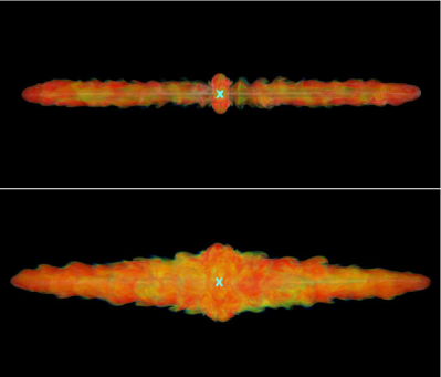
Figure 4: Jet “backflow” cocoons formed by $\mathcal{M}_{j}=3.5$ (Top) and $\mathcal{M}_{j}=10$ (Bottom) steady jets. A passive, jet mass-fraction tracer is volumed rendered in the images. The jets are “in the plane of the sky” and shown when they have approximately the same lengths, $\ell_{j}$. The location of the AGN is marked by an ‘X’. See text for details.

The energy deposition from the jet into the cocoon will generally drive a shock laterally outward into the ICM. We will call this the “inflation shock”. Provided the jet terminus propagates supersonically into the ICM ($\mathcal{M}_{h}\mp\mathcal{M}_{w,\parallel}>1$, equation 15) there will be a bow shock attached to the jet head, which will generally merge with the inflation shock. In Figure 4 the tips of the two cocoons are confined by bow shocks. The tighter “Mach cone” of the higher Mach number jet leads to “sharper points” in the cocoons. Although the bow shock may be quite strong, both observations and simulations suggest that the inflation shock is typically rather weak. For example the $\mathcal{M}_{j}=10$ jets shown in the bottom of Figure 4 and in Figure 5 produce bow shocks with $\mathcal{M}_{h}\approx 7$ ($v_{w,\parallel}=0$) on the nose of the jet in agreement with expectations from equation 16. On the other hand, over much of their surfaces the accompanying both inflation shocks have Mach numbers, $\mathcal{M}\raise 1.29167pt\hbox{$<$}\kern-7.5pt{\lower 2.79857pt\hbox{$\sim$}}1.5$ for the duration of the simulation (see Figure 5). There is no fixed value, however. The relatively small Mach numbers of most of the inflation shock surfaces also point to the fact that the pressure inside the shocks and inside the cocoons is not much greater than the ambient pressure, $P_{i}$ (see equation 20).

Because these properties do not inherently lead to scale-free structures, we do not try to model cocoon formation in terms of self-similar behavior falle91 ; ka97 .

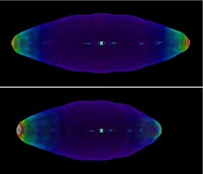
Figure 5: Volume rendering of the shocks associated with the $\mathcal{M}_{j}=10$ simulation shown in the bottom image of Figure 4. The Top image matches the orientation of the bottom image in Figure 4, while the Bottom image has the jet axis rotated 40 degrees, with the left jet approaching (so similar to Figures 2 and 3. Shocks are color coded, with the strongest shocks, $\mathcal{M}_{s}\approx 7$ shown in white, with $\mathcal{M}_{s}\approx 1.5$ represented by purple. ’X’ marks AGN location. See text for details.

Still, it makes sense to estimate the volume of the cocoon simply by comparing the work required to inflate the cocoon to the energy that has passed down the jet into the cocoon. Very simply, we set $P_{i}V_{c}(t)=K_{w}\int L_{j}dt=K_{w}\langle L_{j}\rangle t$, where $K_{w}<1$ is a numerical factor that accounts for energy lost by the cocoon plasma as it inflated. Accounting for adiabatic work done on the ICM would lead to $K_{w}=(\gamma_{j}-1)/\gamma_{j}$. For a non-relativistic jet with $\gamma_{j}=5/3$, this would give $K_{w}=2/5$, while for a jet with a relativistic EoS and $\gamma_{j}=4/3$, the equivalent consequences would give $K_{w}=1/4$. Empirical estimates from non-relativistic simulations do, indeed, suggest $K_{w}\sim 1/2$.oj10 The exact value for $K_{w}$ is not essential to our purposes here.

As a primitive model for cocoon geometry we assume the cocoon length is set by $\int v_{h}(t)dt=\langle v_{h}\rangle t$, giving

$$V_{c}=\langle v_{h}\rangle A_{c}\approx\frac{K_{w}\langle L_{j}\rangle}{P_{i}},$$ (29)

where $A_{c}$ represents a characteristic cocoon cross sectional area. We do not imply in this that the cocoon cross section is constant, and, indeed, it generally will not be (see Figure 4). In practice we treat it as a geometric average cross section.

To simplify our treatment further, we express the jet luminosity in the form applicable to both relativistic and non-relativistic jets suggested by equations 11 and 12; that is,

$$L_{j}\approx\alpha_{j}\mathcal{M}_{j}^{2}v_{j}P_{j}A_{j},$$ (30)

where $1\leq\alpha\leq 2$. For a relativistic jet $v_{j}\to c$ in this expression. From equation 16 we write

$$v_{h}\approx a_{i}\mathcal{M}_{j}\sqrt{\frac{A_{j}}{A_{h}}}\sqrt{\frac{P_{j}}{P_{i}}}\sqrt{\frac{\gamma^{\prime}}{\gamma_{i}}}$$ (31)

Combining equations 29, 30 and 31 gives a simple estimate for $A_{c}$,

$$A_{c}\approx\sqrt{A_{j}A_{h}}~{}\mathcal{M}_{j}\frac{v_{j}}{a_{j}}\sqrt{\frac{a_{j}^{2}\gamma_{i}}{a_{i}^{2}\gamma^{\prime}}}\sqrt{\frac{P_{j}}{P_{i}}}~{}(\alpha K_{w}).$$ (32)

We expect $\alpha K_{w}\raise 1.29167pt\hbox{$<$}\kern-7.5pt{\lower 2.79857pt\hbox{$\sim$}}1$, and, indeed using equation 34, below, and the simulation parameters for the cocoons shown in Figure 4 we get consistent estimates for $A_{c}$ using $\alpha K_{w}\sim 1/2$. Note that, if these various jet parameters are time independent, the effective cocoon cross section, $A_{c}$ is steady in time. That is, the ratio $A_{c}/\ell_{j}\propto 1/t$. We briefly address alternative possibilities below.

For a relativistic jet with a relativistic EoS, $v_{j}/a_{j}\to\sqrt{3}$, while $\tilde{w}_{j}\to 4P_{j}/(\rho_{j}c^{2})$, and equation 32 becomes,

$$A_{c}\approx\sqrt{A_{j}A_{h}}~{}\mathcal{M}_{j}\left(\sqrt{\frac{\rho_{i}}{\rho_{j}}}~{}\frac{P_{j}}{P_{i}}\right)\sqrt{\frac{\rho_{j}c^{2}}{2P_{j}}}~{}(\alpha K_{w})$$ (33)

$$=\sqrt{A_{j}A_{h}}~{}\mathcal{M}_{j}\sqrt{\frac{P_{j}}{P_{i}}}\sqrt{\gamma_{i}}\frac{c}{a_{i}}~{}(\alpha K_{w}).$$

while for a non-relativistic jet,

$$A_{c}\approx\sqrt{A_{j}A_{h}}~{}\mathcal{M}_{j}^{2}\left(\sqrt{\frac{\rho_{i}}{\rho_{j}}}~{}\frac{P_{j}}{P_{i}}\right)~{}(\alpha K_{w}).$$ (34)

The only difference between equations 33 and 34 is a relative factor $(1/\mathcal{M}_{j})\sqrt{\rho_{j}c^{2}/(2P_{j})}$ in equation 33.

We can see from these relations that the cocoon cross section scales with the geometric mean of the jet cross section, $A_{j}$ and the jet head cross section, $A_{h}$. It is strongly boosted if the jet Mach number is large (especially for non-relativistic jets), and, with less sensitivity, to a large density contrast between the ICM and the jet, $\rho_{i}/\rho_{j}$. That is, cocoons will be somewhat fatter for jets with larger density contrast, $\rho_{i}/\rho_{j}$, but especially fatter for larger Mach numbers. We are assuming in these comments that, as argued previously, we should expect $P_{j}/P_{i}\sim 1$. The Mach number sensitivity of $A_{c}$ is evident in a comparison of the non-relativistic jet cocoons shown in Figure 4, where the only difference in the two simulations was jet Mach number; above, $\mathcal{M}_{j}=3.5$, while below, $\mathcal{M}_{j}=10$. The $\mathcal{M}_{j}=10$ cocoon, in particular, is, as noted above, strongly tapered, representing the fact that the Mach cone at its nose has strongly confined it. We associate $A_{c}$ with the mean cross sectional area, which here would be roughly midway between the AGN and the jet terminus.

The reader may have noticed at the same time that the cocoons from the jets shown in Figure 4 are relatively skinny compared to typical, observed radio galaxy cocoons. That is characteristic of the properties of moderate Mach number, non-relativistic AGN jet simulations that are steady and maintain a precise axis for the jets. On the other hand, if either the jet power cycles substantially or the axis of the jet wanders or precesses, the relative rate at which the jet advances is reduced oj10 . In order to maintain the same cocoon volume indicated in equation 29 the cross section must increase. This effect can, be roughly accounted for in equations 31 - 34 by adjusting the effective head area, $A_{h}$. For instance, a precessing jet will balance its thrust during a precession period over an area, $A_{h}\sim 4\pi r_{j}\ell_{j}\gg\pi r_{j}^{2}$, where $\ell_{j}=\ell_{j}(t)$ is the instantaneous length of the jet. Applied into equation 31 the head advance rate, $v_{h}=d\ell_{j}/dt\propto 1/t^{1/2}$. If we maintain constant jet luminosity, $V_{c}\propto t$, so $A_{c}\propto t^{1/2}$. Now, $A_{c}/\ell_{j}=$ const, rather than $A_{c}/\ell_{j}\propto 1/t$. Simultaneously, the volume swept out by the precessing jet itself will be $\sim\ell_{j}^{3}\sin{\theta}\sin{2\theta}$, where $\theta$ is the opening angle of the precession cone. This sets a scale for the effective $A_{c}\sim 2~{}\ell_{j}^{2}\sin{\theta}^{2}$. These effects both fatten the cocoons relative to what we derived above.

Finally, we mention that equation 33 predicts rather fat cocoons for high Mach number relativistic jets propagating in an environment where $c\gg a_{i}$. That is consistent with results of numerical simulations of relativistic hydrodynamical jets pm07 , and also simulations of jets dominated by their Poynting flux (so, internally highly relativistic) li06 .

V Summary

The plasma media in galaxy clusters, ICMs, are dynamical. They are stirred by many processes associated with cluster assembly. The dynamical state of an ICM provides unique information about how this takes place, so it is important to find and evaluate ICM dynamical conditions, especially those far away from equilibrium. X-ray observations can reveal critical information about ICM thermodynamical properties, some statistical characteristics of ICM dynamical states and find relatively strong shocks in higher density ICM regions.

But, much of the story is not visible in the X-ray window. On the other hand, AGNs in so-called “radio mode” are common in clusters, and especially in disturbed clusters. Those AGNs expel fast plasma jets that plow through the ICM. Those interactions will influence the ICM and its evolution. More to the point of this paper, however, is the considerable impact of ICM dynamics on the trajectories and of the AGN jets and the distributions of their debris. In particular, impacts between ICM shocks and winds will distort and even disrupt the AGN structures that form. Through an understanding of how those distortions develop and how they depend on the AGN and ICM properties we hope to open a clearer window to revealing the dynamical structures of ICMs. By relating those structures to other information about the dynamical state of the cluster, and, for instance, evidence for merging, strong accretion events or gravitational disturbance by dark matter halos, these insights can provide vital probes of cluster formation processes and their relative roles.

We have laid out in this paper a simple summary of some of the essential dynamical relationships involved in AGN/ICM interactions, with a special focus on interactions involving ICM shocks. The nominal target application is ICM shocks colliding with AGN outflows. We pointed out, however, that the relations we developed have application to any relative motion between the AGN and its immediate environment. The formalism allows AGN jets that are either non-relativistic or relativistic.

We set down basic relations to evaluate shock interactions with the low density cavities created by AGN jets, as well as to follow the propagation of the jets within post-shock flows. For completeness, we used the same formalism to provide a basic context for the formation of the cavities themselves. One notable aspect of the relationships we derive is the essential roles of the internal Mach number of the jet flow and the Mach number of the ICM shock. More directly, the ratio of these two Mach numbers seems central to evaluating the interactions between the AGN and a dynamical ambient environment. This provides a potentially useful link that can help develop quantitative understandings of ICM dynamical states that otherwise are likely to remain obscure for some time.

- (1) A. Kravtsov & S. Borgani, “Formation of Galaxy Clusters”, ARAA 50, 353-409 (2012)
- (2) F. Vazza, T. W. Jones, M. Bruggen, G. Brunetti, D. Porter & D. Ryu, “Turbulence and Vorticity in Galaxy Clusters Generated by Structure Formation”, MNRAS (in press) (arXiv:1609.03558)
- (3) E. Zinger, A, Dekel, Y. Birnboim, A. Kravtsov & D. Nagai, “The Role of Penetrating Gas Streams in Setting the Dynamical State of Galaxy Clusters” MNRAS 461, 412-432 (2016)
- (4) A. Schekochihin & S. Cowley, “Turbulence, Magnetic Fields and Plasma Physics in Clusters of Galaxies”, Phys. Plasmas 13, 56501-56508 (2006)
- (5) M. Markevitch & A. Vikhlinin, “Shocks and Cold Fronts in Galaxy Clusters”, Phys. Rep. 443, 1-53 (2007)
- (6) S. Walker, J. Sanders & A. Fabian, “Constraining Gas Motions in the Centaurus Cluster Using X-ray Surface Brightness Fluctuations and Metal Diffusion”, MNRAS 453, 3699-3705 (2015)
- (7) The Hitomi Collaboration, “The Quiescent Intracluster Medium in the Core of the Perseus Cluster”, Nature 535, 117-121 (2016)
- (8) R. Adam, B. Comis, I. Bartalucci, A. Adane, P. Ade, P. Andre, A. Beelen, A. Benoit, A. Bideaud, N. Billot, O. Bourrion, M. Calvo, A. Catalano, G. Coiffard, A. D’Addabbo, F. Desert, S. Doyle, J. Goupy, B. Hasnoun, I. Hermelo, C. Kramer, G. Lagache, S. Leclercq, J. Macias-Perez, J. Martino, P. Mauskopf, F. Mayet, A. Monfardini, F. Pajot, E. Pascale, L. Perotto, E. Pointecouteau, N. Pnthieu, G. Pratt, V. Reveret, A. Ritacco, L. Rodrigues, G. Savini, K. Schuster, A. Sievers, S. Triqueneaux, C. Tucker & R. Zylka, “High Angular Resolution Sunyaev-Zel’dovich Observations of MACS J1423.8+2404 with NIKA: Multi-wavelength Analysis”, A.& A. 586, 122-138 (2016)
- (9) G. Brunetti & T. W. Jones, “Cosmic Rays in Galaxy Clusters and Their Nonthermal Emission”, Int.J.Mod.Phys. (D) 23, 430007-430083 (2014)
- (10) A. Pinzke, P. Oh & C. Pfrommer, “Turbulence and Particle Acceleration in Giant Radio Halos: the Origin of Seed Electrons”, arXiv150307870P (2015)
- (11) H. Kang & D. Ryu, “Curved Radio Spectra of Weak Cluster Shocks”, Ap.J. 809, 186-202 (2015)
- (12) J. Donnert, A. Stroe, G. Brunetti, D. Hoang & H. Roettgering, “Magnetic Field Evolution in Giant Radio Relics Using the Example of CIZA J2242.8+5301, MNRAS, 462, 2014-2032 (2016)
- (13) M. Ledlow & F. Owen, “20 CM LVA Survey of Abell Clusters of Galaxies. VI. Radio/Optical Luminosity Functions”, A. J. 112, 9-22 (1996)
- (14) N. Malavasi, S. Bardelli, P. Ciliegi, O. Ilbert, L. Pozzetti & E. Zucca, “The Environment of Radio Sources in the VLA-COSMOS Survey”, arXiv:1609.02178 (2016)
- (15) Y. Li, G. Bryan, M. Ruszkowski, G. Voit, B. O’Shea, M. Donahue, “Cooling, AGN Feedback and Star Formation in Simulated Cool-core Galaxy Clusters”, Ap. J. 811, 73-88 (2015)
- (16) M. Ryle & M. Windram, “The Radio Emission from Galaxies in the Perseus Cluster”, MNRAS 138, 1-21 (1968)
- (17) F. Owen & L. Rudnick, “Radio Sources with Wide-Angle Tails in Abell Clusters of Galaxies”, Ap.J. 205, L1-L4 (1976)
- (18) M. Bliton, E. Rizza, J. Burns, F. Owen & M. Ledlow, “Cluster-subcluster Mergers and the Formation of Narrow-angle Tailed Radio Galaxies”, MNRAS, 301, 609-625 (1998)
- (19) I. Sakelliou & M. Merrifield, “The Origin of Wide-angle Tailed Radio Galaxies”, MNRAS, 311, 649-656 (2000)
- (20) M. Begelman, M. Rees & R. Blandford, “A Twin-jet Model for Radio Tails”, Nature 279, 770-773 (1979)
- (21) Z. Mguda, A. Faltenbacher, K. van der Heyden, S. Gottlober, C. Cress, P. Vaisanen & G. Vepes, “Ram Pressure Statistics for Bent Tail Radio Galaxies”, MNRAS 446, 3310-3318 (2015)
- (22) T. Ensslin & M. Bruggen, “On the Formation of Cluster Radio Relics”, MNRAS 331, 1011-1019 (2002)
- (23) C. Pfrommer & T. W. Jones, “Radio Galaxy NGC 1265 Unveils the Accretion Shock Onto the Perseus Galaxy Cluster”, Ap.J. 730, 22-34 (2011)
- (24) A. Bonafede, H. Intema, M. Bruggen, M. Girardi, M. Nonino, N. Kantharia, R. van Weeren & H. Rottgering, “Evidence for Particle Re-acceleration in the Radio Relic in the Galaxy Cluster PLCKG287.0+32.9”, Ap.J. 785, 1-14 (2014)
- (25) P. Mendygral, N. Radcliffe, K. Kandalla, D. Porter, B. O’Neill, C. Nolting, P. Edmon, J. Donnert & T. Jones “WOMBAT: A Scalable and High Performance Astrophysical MHD Code”, ApJS (submitted)
- (26) M. Begelman, R. Blandford & M. Rees, “Theory of Extragalactic Radio Sources”, Rev. Mod. Phys. 56, 255- (1984)
- (27) D. Ryu, H. Kang, E. Hallman & T. W. Jones, “Cosmological Shock Waves and Their Role in the Large-Scale Structure of the Universe”, Ap.J. 593, 599-610 (2003)
- (28) D. Porter, T. W. Jones & D. Ryu, “Vorticity, Shocks and Magnetic Fields in Subsonic, ICM-like Turbulence”, Ap.J. 810, 93-211 (2015)
- (29) L. Landau & E. Lifshitz, Fluid Mechanics (Elsevier Science) (1987)
- (30) A. Konigl, “Relativistic Gasdynamics in Two Dimensions”, Phys. Fluids 23, 1083-1092 (1980)
- (31) H. Roettgering, I. Snellen, G. Miley, J. de Jong, R. Hanisch & R. Perley, “VLA Observations of the Rich X-ray Cluster Abell 2256”, Ap.J. 436, 654-668 (1994)
- (32) F. Owen, L. Rudnick, J. Eilek, U. Rau, S. Bhatnagar & L. Kogan, “Wideband VLA Observations of Abell 2256 I: Continuum, Rotation Measure and Spectral Imaging”, Ap.J. 794, 24-38 (2014)
- (33) C. O’Dea & F. Owen, “Multifrequency VLA Observations of the Prototypical Narrow-Angle Tail Radio Source NGC 1265”, Ap. J. 301, 841-859 (1986)
- (34) M. Ruszkowski, T. Ensslin, M. Bruggen, S. Heinz & C, Pfrommer, “Impact of Tangled Magnetic Fields on Fossil Radio Bubbles”, MNRAS 378, 662-672 (2007)
- (35) S. O’Neill, D. de Young & T. W. Jones, “Three-Dimensional Magnetohydrodynamical Simulations of Buoyant Bubbles in Galaxy Clusters”, Ap. J. 694, 1317-1330 (2009)
- (36) S. Falle, “Self-Similar Jets”, MNRAS 250, 581-596 (1991)
- (37) C. Kaiser & P. Alexander, “A Self-Similar Model for Extragalactic Radio Sources”, MNRAS 286, 215-222 (1997)
- (38) S. O’Neill & T. W. Jones, “Three Dimensional Simulations of Bi-directed Magnetohydrodynamical Jets Interacting with Cluster Environments”, Ap.J. 710, 180-196 (2010)
- (39) M. Perucho & J. Marti, “A Numerical Simulation of the Evolution and Fate of a Fanaroff-Riley Type I Jet. The Case of 3C 31”, MNRAS 382, 526-542 (2007)
- (40) H. Li, L. Giovanni, J. Finn, S. Li & S. Colgate, “Modeling the Large-Scale Structures of Astrophysical Jets in the Magnetically Dominated Limit”, Ap.J. 643, 92-100 (2006)