Optimal Target Assignment and Path Finding
for Teams of Agents

Abstract

We study the TAPF (combined target-assignment and path-finding) problem for teams of agents in known terrain, which generalizes both the anonymous and non-anonymous multi-agent path-finding problems. Each of the teams is given the same number of targets as there are agents in the team. Each agent has to move to exactly one target given to its team such that all targets are visited. The TAPF problem is to first assign agents to targets and then plan collision-free paths for the agents to their targets in a way such that the makespan is minimized. We present the CBM (Conflict-Based Min-Cost-Flow) algorithm, a hierarchical algorithm that solves TAPF instances optimally by combining ideas from anonymous and non-anonymous multi-agent path-finding algorithms. On the low level, CBM uses a min-cost max-flow algorithm on a time-expanded network to assign all agents in a single team to targets and plan their paths. On the high level, CBM uses conflict-based search to resolve collisions among agents in different teams. Theoretically, we prove that CBM is correct, complete and optimal. Experimentally, we show the scalability of CBM to TAPF instances with dozens of teams and hundreds of agents and adapt it to a simulated warehouse system.

I.2.8Artificial IntelligenceProblem Solving, Control Methods, and Search[graph and tree search strategies, heuristic methods] I.2.11Artificial IntelligenceDistributed Artificial Intelligence[intelligent agents, multi-agent systems]

Algorithms, Performance, Experimentation

¡ccs2012¿ ¡concept¿ ¡concept_id¿10010147.10010178.10010199¡/concept_id¿ ¡concept_desc¿Computing methodologies Planning and scheduling¡/concept_desc¿ ¡concept_significance¿500¡/concept_significance¿ ¡/concept¿ ¡concept¿ ¡concept_id¿10010147.10010178.10010199.10010202¡/concept_id¿ ¡concept_desc¿Computing methodologies Multi-agent planning¡/concept_desc¿ ¡concept_significance¿500¡/concept_significance¿ ¡/concept¿ ¡concept¿ ¡concept_id¿10010147.10010178.10010219.10010220¡/concept_id¿ ¡concept_desc¿Computing methodologies Multi-agent systems¡/concept_desc¿ ¡concept_significance¿500¡/concept_significance¿ ¡/concept¿ ¡concept¿ ¡concept_id¿10010147.10010178.10010219.10010221¡/concept_id¿ ¡concept_desc¿Computing methodologies Intelligent agents¡/concept_desc¿ ¡concept_significance¿500¡/concept_significance¿ ¡/concept¿ ¡concept¿ ¡concept_id¿10010147.10010178.10010199.10010200¡/concept_id¿ ¡concept_desc¿Computing methodologies Planning for deterministic actions¡/concept_desc¿ ¡concept_significance¿300¡/concept_significance¿ ¡/concept¿ ¡concept¿ ¡concept_id¿10010147.10010178.10010199.10010204¡/concept_id¿ ¡concept_desc¿Computing methodologies Robotic planning¡/concept_desc¿ ¡concept_significance¿300¡/concept_significance¿ ¡/concept¿ ¡concept¿ ¡concept_id¿10010147.10010178.10010205.10010207¡/concept_id¿ ¡concept_desc¿Computing methodologies Discrete space search¡/concept_desc¿ ¡concept_significance¿300¡/concept_significance¿ ¡/concept¿ ¡concept¿ ¡concept_id¿10010147.10010178.10010213.10010215¡/concept_id¿ ¡concept_desc¿Computing methodologies Motion path planning¡/concept_desc¿ ¡concept_significance¿300¡/concept_significance¿ ¡/concept¿ ¡concept¿ ¡concept_id¿10002950.10003624.10003633.10003644¡/concept_id¿ ¡concept_desc¿Mathematics of computing Network flows¡/concept_desc¿ ¡concept_significance¿300¡/concept_significance¿ ¡/concept¿ ¡concept¿ ¡concept_id¿10003752.10003809.10003635.10010037¡/concept_id¿ ¡concept_desc¿Theory of computation Shortest paths¡/concept_desc¿ ¡concept_significance¿300¡/concept_significance¿ ¡/concept¿ ¡concept¿ ¡concept_id¿10010520.10010553.10010554.10010557¡/concept_id¿ ¡concept_desc¿Computer systems organization Robotic autonomy¡/concept_desc¿ ¡concept_significance¿300¡/concept_significance¿ ¡/concept¿ ¡/ccs2012¿

[500]Computing methodologies Planning and scheduling [500]Computing methodologies Multi-agent planning [500]Computing methodologies Multi-agent systems [500]Computing methodologies Intelligent agents [300]Computing methodologies Planning for deterministic actions [300]Computing methodologies Robotic planning [300]Computing methodologies Discrete space search [300]Computing methodologies Motion path planning [300]Mathematics of computing Network flows [300]Theory of computation Shortest paths [300]Computer systems organization Robotic autonomy

1 Introduction

Teams of agents often have to assign targets among themselves and then plan collision-free paths to their targets. Examples include autonomous aircraft towing vehicles airporttug16 , automated warehouse systems kiva , office robots DBLP:conf/ijcai/VelosoBCR15 and game characters in video games WHCA . For example, in the near future, autonomous aircraft towing vehicles might tow aircraft all the way from the runways to their gates (and vice versa), reducing pollution, energy consumption, congestion and human workload. Today, autonomous warehouse robots already move inventory pods all the way from their storage locations to the inventory stations that need the products they store (and vice versa), see Figure 1.

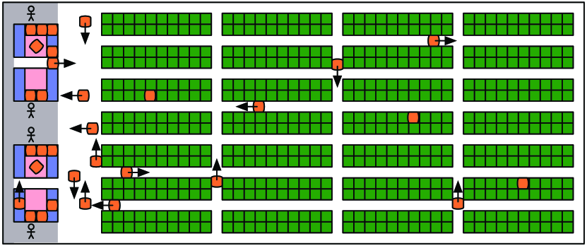
Figure 1: A typical Kiva warehouse system kiva .

We therefore study the TAPF (combined target-assignment and path-finding) problem for teams of agents in known terrain. The agents are partitioned into teams. Each team is given the same number of unique targets (goal locations) as there are agents in the team. The TAPF problem is to assign agents to targets and plan collision-free paths for the agents from their current locations to their targets in a way such that each agent moves to exactly one target given to its team, all targets are visited and the makespan (the earliest time step when all agents have reached their targets and stop moving) is minimized. Any agent in a team can be assigned to a target of the team, and the agents in the same team are thus exchangeable. However, agents in different teams are not exchangeable.

1.1 Related Work

The TAPF problem generalizes the anonymous and non-anonymous MAPF (multi-agent path-finding) problems:

• The anonymous MAPF problem (sometimes called goal-invariant MAPF problem) results from the TAPF problem if only one team exists (that consists of all agents). It is called “anonymous” because any agent can be assigned to a target, and the agents are thus exchangeable. The anonymous MAPF problem can be solved optimally in polynomial time YuLav13STAR . Anonymous MAPF solvers use, for example, the polynomial-time max-flow algorithm on a time-expanded network YuLav13STAR (an idea that originated in the operations research literature SurveyDinaymicFlow ) or graph-theoretic algorithms AAAI15-MacAlpine .

• The non-anonymous MAPF problem (often just called MAPF problem) results from the TAPF problem if every team consists of exactly one agent and the number of teams thus equals the number of agents. It is called “non-anonymous” because only one agent can be assigned to a target (meaning that the assignments of agents to targets are pre-determined), and the agents are thus non-exchangeable. The non-anonymous MAPF problem is NP-hard to solve optimally and even NP-hard to approximate within any constant factor less than 4/3 MaAAAI16 . Non-anonymous MAPF solvers use, for example, reductions to problems from satisfiability, integer linear programming or answer set programming  YuLav13ICRA ; erdem2013general ; Surynek15 or optimal, bounded suboptimal or suboptimal search algorithms ODA ; EPEJAIR ; MStar ; DBLP:journals/ai/SharonSGF13 ; ICBS ; PushAndSwap ; PushAndRotate ; ECBS ; DBLP:conf/socs/CohenUK15 , such as the optimal CBS (conflict-based search) algorithm DBLP:journals/ai/SharonSFS15 .

Research so far has concentrated on these two extreme cases. Yet, many real-world applications fall between the extreme cases because the number of teams is larger than one but smaller than the number of agents, which is why we study the TAPF problem in this paper. The TAPF problem is NP-hard to solve optimally and even NP-hard to approximate within any constant factor less than 4/3 if more than one team exists MaAAAI16 . It is unclear how to generalize anonymous MAPF algorithms to solving the TAPF problem. Straightforward ways of generalizing non-anonymous MAPF algorithms to solving the TAPF problem have difficulties with either scalability (due to the resulting large state spaces), such as searching over all assignments of agents to targets to find optimal solutions, or solution quality, such as assigning agents to targets with algorithms such as Tovey2005 ; ZhengIJCAI and then planning collision-free paths for the agents with non-anonymous MAPF algorithms (perhaps followed by improving the assignment and iterating WagnerSoCS12 ) to find sub-optimal solutions.

1.2 Contribution

We present the CBM (Conflict-Based Min-Cost-Flow) algorithm to bridge the gap between the extreme cases of anonymous and non-anonymous MAPF problems. CBM solves the TAPF problem optimally by simultaneously assigning agents to targets and planning collision-free paths for them, while utilizing the polynomial-time complexity of solving the anonymous MAPF problem for all agents in a team to scale to a large number of agents. CBM is a hierarchical algorithm that combines ideas from anonymous and non-anonymous MAPF algorithms. It uses CBS on the high level and a min-cost max-flow algorithm Successive on a time-expanded network on the low level. Theoretically, we prove that CBM is correct, complete and optimal. Experimentally, we show the scalability of CBM to TAPF instances with dozens of teams and hundreds of agents and adapt it to a simulated warehouse system.

2 TAPF

In this section, we formalize the TAPF problem and show how it can be solved via a reduction to the integer multi-commodity flow problem on a time-expanded network.

2.1 Definition and Properties

For a TAPF instance, we are given an undirected connected graph $G=(V,E)$ (whose vertices $V$ correspond to locations and whose edges $E$ correspond to ways of moving between locations) and $K$ teams $team_{1}\ldots team_{K}$. Each team $team_{i}$ consists of $K_{i}$ agents $a^{i}_{1}\ldots a^{i}_{K_{i}}$. Each agent $a^{i}_{j}$ has a unique start vertex $s^{i}_{j}$. Each team $team_{i}$ is given unique targets (goal vertices) $g^{i}_{1}\ldots g^{i}_{K_{i}}$. Each agent $a^{i}_{j}$ must move to a unique target $g^{i}_{j^{\prime}}$. An assignment of agents in team $team_{i}$ to targets is thus a one-to-one mapping $\varphi^{i}$, determined by a permutation on $1\ldots K_{i}$, that maps each agent $a^{i}_{j}$ in $team_{i}$ to a unique target $g^{i}_{j^{\prime}}=\varphi^{i}(a^{i}_{j})$ of the same team. A path for agent $a^{i}_{j}$ is given by a function $l^{i}_{j}$ that maps each integer time step $t=0\ldots\infty$ to the vertex $l^{i}_{j}(t)\in V$ of the agent in time step $t$. A solution consists of paths for all agents that obey the following conditions:

1. $\forall i,j:\leavevmode\nobreak\ l^{i}_{j}(0)=s^{i}_{j}$ (each agent starts at its start vertex);

2. $\forall i,j\leavevmode\nobreak\ \exists\mbox{a minimal}\leavevmode\nobreak\ T^{i}_{j}\leavevmode\nobreak\ \forall t\geq T^{i}_{j}:\leavevmode\nobreak\ l^{i}_{j}(t)=\varphi^{i}(a^{i}_{j})$ (each agent ends at its target);

3. $\forall i,j,t:\leavevmode\nobreak\ (l^{i}_{j}(t)=l^{i}_{j}(t+1)$ or $(l^{i}_{j}(t),l^{i}_{j}(t+1))\in E)$ (each agent always stays at its current vertex or moves to an adjacent vertex);

4. $\forall a^{i}_{j},a^{i^{\prime}}_{j^{\prime}},t\leavevmode\nobreak\ \mbox{with}\leavevmode\nobreak\ a^{i}_{j}\neq a^{i^{\prime}}_{j^{\prime}}:l^{i}_{j}(t)\neq l^{i^{\prime}}_{j^{\prime}}(t)$ (there are no vertex collisions since different agents never occupy the same vertex at the same time);

5. $\forall a^{i}_{j},a^{i^{\prime}}_{j^{\prime}},t\leavevmode\nobreak\ \mbox{with}\leavevmode\nobreak\ a^{i}_{j}\neq a^{i^{\prime}}_{j^{\prime}}:(l^{i}_{j}(t)\neq l^{i^{\prime}}_{j^{\prime}}(t+1)$ or $l^{i^{\prime}}_{j^{\prime}}(t)\neq l^{i}_{j}(t+1))$ (there are no edge collisions since different agents never move along the same edge in different directions at the same time).

Given paths for all agents in team $team_{i}$, the team cost of team $team_{i}$ is $\max_{j}T^{i}_{j}$ (the earliest time step when all agents in the team have reached their targets and stop moving). Given paths for all agents, the makespan is $\max_{i,j}T^{i}_{j}$ (the earliest time step when all agents have reached their targets and stop moving). The task is to find an optimal solution, namely one with minimal makespan. Note that a (non-anonymous) MAPF instance can be obtained from a TAPF instance by fixing the assignments of agents to targets. Any solution of a TAPF instance is thus also a solution of a (non-anonymous) MAPF instance on the same graph for a suitable assignment of agents to targets. Since the makespan of any optimal (non-anonymous) MAPF solution is bounded by $O(|V|^{3})$ YuR14 , the makespan of any optimal TAPF solution is also bounded by $O(|V|^{3})$.

We define a collision between an agent agent $a^{i}_{j}$ in team $team_{i}$ and a different agent $a^{i^{\prime}}_{j^{\prime}}$ in team $team_{i^{\prime}}$ to be either a vertex collision ($team_{i}$, $team_{i^{\prime}}$, $l$, $t$) [if $l=l^{i}_{j}(t)=l^{i^{\prime}}_{j^{\prime}}(t)$ and thus both agents occupy the same vertex at the same time] or an edge collision ($team_{i}$, $team_{i^{\prime}}$, $l_{1}$, $l_{2}$, $t$) [if $l_{1}=l^{i}_{j}(t)=l^{i^{\prime}}_{j^{\prime}}(t+1)$ and $l_{2}=l^{i^{\prime}}_{j^{\prime}}(t)=l^{i}_{j}(t+1)$ and thus both agents move along the same edge in different directions at the same time]. Likewise, we define a constraint to be either a vertex constraint ($team_{i}$, $l$, $t$) [that prohibits any agent in $team_{i}$ from occupying vertex $l$ in time step $t$] or an edge constraint ($team_{i}$, $l_{1}$, $l_{2}$, $t$) [that prohibits any agent in team $team_{i}$ from moving from vertex $l_{1}$ to vertex $l_{2}$ between time steps $t$ and $t+1$].

2.2 Solution via Reduction to Flow Problem

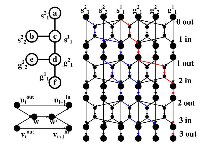
Figure 2: An example of constructing and finding a feasible integer multi-commodity flow for a 3-step time-expanded network. The TAPF instance consists of two teams. Team 1 consists of agent $\{a^{1}_{1}\}$ with target $\{g^{1}_{1}\}$. Team 2 consists of agents $\{a^{2}_{1},a^{2}_{2}\}$ with targets $\{g^{2}_{1},g^{2}_{2}\}$. The red edges represents a flow for commodity type 1, which corresponds to a path for the agent in Team 1. The blue edges represent a flow for commodity type 2, which corresponds to paths for the two agents in Team 2. The flow thus corresponds to an assignment of agent $a^{1}_{1}$ to target $g^{1}_{1}$, agent $a^{2}_{1}$ to target $g^{2}_{2}$ and agent $a^{2}_{2}$ to target $g^{2}_{1}$ as well as the (optimal) solution $\{\langle c,d,f,f\rangle\}$ and $\{\langle a,c,d,e\rangle,\langle b,b,c,d\rangle\}$.

Given a TAPF instance on undirected graph $G=(V,E)$ and a limit $T$ on the number of time steps, we construct a $T$-step time-extended network using a reduction that is similar to that from the (non-anonymous) MAPF problem to the integer multi-commodity flow problem YuLav13ICRA (the idea of which is an extension of YuLav13STAR ). A $T$-step time-extended network is a directed network $\mathcal{N}=(\mathcal{V},\mathcal{E})$ with vertices $\mathcal{V}$ and directed edges $\mathcal{E}$ that have unit capacity. Each vertex $v\in V$ is translated to a vertex $v_{t}^{out}\in\mathcal{V}$ for all $t=0\ldots T$ (which represents vertex $v$ at the end of time step $t$) and a vertex $v_{t}^{in}\in\mathcal{V}$ for all $t=1\ldots T$ (which represents vertex $v$ in the beginning of time step $t$). There is a supply of one unit of commodity type $i$ at vertex ${(s^{i}_{j})}_{0}^{out}$ and a demand of one unit of commodity type $i$ at vertex ${(g^{i}_{j})}^{out}_{T}$ for all $i=1\ldots K$ and $j=1\ldots K_{i}$. Each vertex $v\in V$ is also translated to an edge $(v_{t}^{out},v_{t+1}^{in})\in\mathcal{E}$ for all $t=0\ldots T-1$ (which represents an agent staying at vertex $v$ between time steps $t$ and $t+1$). Each vertex $v\in V$ is also translated to an edge $(v_{t}^{in},v_{t}^{out})\in\mathcal{E}$ for all $t=1\ldots T$ (which prevents vertex collisions of the form $(*,*,v,t)$ among all agents since only one agent can occupy vertex $v$ between time steps $t$ and $t+1$). Each edge $(u,v)\in E$ is translated to a gadget of vertices in $\mathcal{V}$ and edges in $\mathcal{E}$ for all $t=0\ldots{T-1}$, which consists of two auxiliary vertices $w,w^{\prime}\in\mathcal{V}$ that are unique to the gadget (but have no subscripts here for ease of readability) and the edges $(u_{t}^{out},w),(v_{t}^{out},w),(w,w^{\prime}),(w^{\prime},u_{t+1}^{in}),(w,v_{t+1}^{in})\in\mathcal{E}$. This gadget prevents edge collisions of the forms $(*,*,u,v,t)$ and $(*,*,v,u,t)$ among all agents since only one agent can move along the edge $(u,v)$ in any direction between time steps $t$ and $t+1$. Figure 2 shows a simple example. The following theorem holds by construction and can be proved in a way similar to the one for the reduction of the (non-anonymous) MAPF problem to the integer multi-commodity flow problem YuLav13ICRA :

Theorem 1.

There is a correspondence between all feasible integer multi-commodity flows on the $T$-step time-extended network of a number of unit that equals the number of agents and all solutions of the TAPF instance with makespans of at most $T$.

An optimal solution can therefore be found by starting with $T=0$ and iteratively checking for increasing values of $T$ whether a feasible integer multi-commodity flow of a number of units that equals the number of agents exists for the corresponding $T$-step time-expanded network (which is an NP-hard problem), until an upper bound on $T$ is reached (such as the one provided in YuR14 ). Each $T$-step time-expanded network is translated in the standard way into an ILP (integer linear program), which is then solved with an ILP algorithm. We evaluate this ILP-based TAPF solver experimentally in Section 4.1. The anonymous MAPF problem results from the TAPF problem if only one team exists (that consists of all agents). The following corollary thus follows from YuLav13STAR :

Corollary 2.

The TAPF problem can be solved optimally in polynomial time if only one team exists.

3 Conflict-Based Min-Cost Flow

In this section, we present the CBM (Conflict-Based Min-Cost-Flow) algorithm, a hierarchical algorithm that solves TAPF instances optimally. On the high level, CBM considers each team to be a meta-agent. It uses CBS to resolve collisions among meta-agents, that is, agents in different teams. CBS is a form of best-first search on a tree, where each node contains a set of constraints and paths for all agents that obey these constraints, move all agents to unique targets of their teams and result in no collisions among agents in the same team. On the low level, CBM uses a polynomial-time min-cost max-flow algorithm Successive on a time-expanded network to assign all agents in a single team to unique targets of the same team and plan paths for them that obey the constraints imposed by the currently considered high-level node and result in no collisions among the agents in the team. Since the running time of CBS on the high level can be exponential in the number of collisions that need to be resolved DBLP:journals/ai/SharonSFS15 , CBM uses edge weights on the low level to bias the search so as to reduce the possibility of creating collisions with agents in different teams.

The idea of biasing the search on the low level has been used before for solving the (non-anonymous) MAPF problem with CBS ECBS . Similarly, the idea of grouping some agents into a meta-agent on the high level and planning paths for each group on the low level has been used before for solving the (non-anonymous) MAPF problem with CBS DBLP:journals/ai/SharonSFS15 but faces the difficulty of having to identify good groups of agents. The best way to group agents can often be determined only experimentally and varies significantly among MAPF instances. On the other hand, grouping all agents in a team into a meta-agent for solving the TAPF problem is a natural way of grouping agents since the assignments of agents in the same team to targets and their paths strongly depend on each other and should therefore be planned together on the low level. For example, if an agent is assigned to a different target, then many of the agents in the same team typically need to be assigned to different targets as well and have their paths re-planned. Also, the lower level can then use a polynomial-time max-flow algorithm on a time-expanded network to assign all agents in a single team to targets and find paths for them due to the polynomial-time complexity of the corresponding anonymous MAPF problem.

3.1 High-Level Search of CBM

1 $Root.constraints\leftarrow\emptyset$;

2 $Root.paths\leftarrow\emptyset$;

3 for each $team_{i}$ do

4       if Lowlevel($team_{i}$, $Root$) returns no paths then

5             return No solution exists;

6            

7      Add the returned paths to $Root.paths$;

8      

9$Root.key\leftarrow$ Makespan($Root.paths$);

10 $Priorityqueue\leftarrow\{Root\}$;

11 while $Priorityqueue\neq\emptyset$ do

12       $N\leftarrow Priorityqueue.pop()$;

13       if Findcollisions($N.paths$) returns no collisions then

14             return Solution is $N.paths$;

15            

16      $Collision\leftarrow$ earliest collision found;

17       for each $team_{i}$ involved in $Collision$ do

18             $N^{\prime}\leftarrow$ Newnode() /* with parent $N$ */;

19             $N^{\prime}.constraints\leftarrow N.constraints$;

20             $N^{\prime}.paths\leftarrow N.paths$;

21             Add one new constraint for $team_{i}$ to $N^{\prime}.constraints$;

22             if Lowlevel($team_{i}$, $N^{\prime}$) returns paths then

23                   Update $N^{\prime}.paths$ with the returned paths;

24                   $N^{\prime}.key\leftarrow$ $max$(Makespan($N^{\prime}.paths$), $N.key$);

25                   $Priorityqueue.insert(N^{\prime})$;

26                  

27            

28      

29return No solution exists;

Algorithm 1 High-Level Search of CBM

On the high level, CBM performs a best-first search on a binary tree, see Algorithm 1. Each node $N$ contains constraints $N.constraints$ and paths for all agents $N.paths$ that obey these constraints, move all agents to unique targets of their teams and result in no collisions among agents in the same team. All nodes are stored in a priority queue. The priority queue initially consists of only the root node $Root$ with no constraints and paths for all agents that move all agents to unique targets of their teams, result in no collisions among agents in the same team and minimize the team cost of each team [Lines 1-8]. If the priority queue is empty, then CBM terminates unsuccessfully [Line 23]. Otherwise, CBM always chooses a node $N$ in the priority queue with the smallest key [Line 10]. The key of a node is the makespan of its paths. (Ties are broken in favor of the node whose paths have the smallest number of colliding teams.) If the paths of node $N$ have no colliding agents, then they are a solution and CBM terminates successfully with these paths [Lines 11-12]. Otherwise, CBM determines all collisions between two agents (which have to be in different teams) and then resolves a collision $Collision$ whose time step $t$ is smallest [Line 13]. (We have evaluated different ways of prioritizing the collisions, including the one suggested in ICBS , but have not observed significant differences in the resulting running times of CBM.) Let the two colliding agents be in $team_{i}$ and $team_{i^{\prime}}$. CBM then generates two child nodes $N_{1}$ and $N_{2}$ of node $N$, both of which inherit the constraints and paths from their parent node [Lines 15-17]. If the collision is a vertex collision $(team_{i},team_{i^{\prime}},l,t)$ or, equivalently, $(team_{i^{\prime}},team_{i},l,t)$, then CBM adds the vertex constraint $(team_{i},l,t)$ to the constraints of node $N_{1}$ and the vertex constraint $(team_{i^{\prime}},l,t)$ to the constraints of node $N_{2}$ [Line 18]. If the collision is an edge collision $(team_{i},team_{i^{\prime}},l_{1},l_{2},t)$ or, equivalently, $(team_{i^{\prime}},team_{i},l_{2},l_{1},t)$, then CBM adds the edge constraint $(team_{i},l_{1},l_{2},t)$ to the constraints of node $N_{1}$ and the edge constraint $(team_{i^{\prime}},l_{2},l_{1},t)$ to the constraints of node $N_{2}$ [Line 18]. For each of the two new nodes, say node $N_{1}$, the low-level search is called to assign all agents in team $team_{i}$ to unique targets of the same team and find paths for them that obey the constraints of node $N_{1}$ and result in no collisions among the agents in the team. If the low-level search successfully returns such paths, then CBM updates the paths of node $N_{1}$ by replacing the paths of all agents in team $team_{i}$ with the returned ones, updates the key of node $N_{1}$ and inserts it into the priority queue [Lines 19-22]. Otherwise, it discards the node.

3.2 Low-Level Search of CBM

On the low level, Lowlevel($team_{i}$,$N$) assigns all agents in team $team_{i}$ to unique targets of the same team and finds paths for them that obey all constraints of node $N$ (namely all vertex constraints of the form ($team_{i}$, *, *) and all edge constraints of the form ($team_{i}$, *, *, *)) and result in no collisions among the agents in the team.

Given a limit $T$ on the number of time steps, CBM constructs the $T$-step time-expanded network from Section 2.2 with the following changes: a) There is only a single commodity type $i$ since CBM considers only the single team $team_{i}$. There is a supply of one unit of this commodity type at vertex ${(s^{i}_{j})}_{0}^{out}$ and a demand of one unit of this commodity type at vertex ${(g^{i}_{j})}^{out}_{T}$ for all $j=1\ldots K_{i}$. b) To obey the vertex constraints, CBM removes the edge $(l^{in}_{t},l^{out}_{t})$ from $\mathcal{E}$ for each vertex constraint of the form $(team_{i},l,t)$. c) To obey the edge constraints, CBM removes the edges $((l_{1})^{out}_{t},w)$ and $(w^{\prime},(l_{2})^{in}_{t+1})$ from $\mathcal{E}$ for all gadgets that correspond to edge $(l_{1},l_{2})\in E$ for each edge constraint of the form $(team_{i},l_{1},l_{2},t)$. Let $\mathcal{V}=\mathcal{V^{\prime}}$ be the set of (remaining) vertices and $\mathcal{E^{\prime}}$ be the set of remaining edges.

Similar to the procedure from Section 2.2, CBM iteratively checks for increasing values of $T$ whether a feasible integer single-commodity flow of $K_{i}$ units exists for the corresponding $T$-step time-expanded network, which can be done with the polynomial-time max-flow algorithm that finds a feasible maximum flow. CBM can start with $T$ being the key of the parent node of node $N$ since it is a lower bound on the new key of node $N$ due to Line 21. (For $N=Root$, CBM starts with $T=0$.) During the earliest iteration when the max-flow algorithm finds a feasible flow of $K_{i}$ units, the call returns successfully with the paths for the agents in the team that correspond to the flow. If $T$ reaches an upper bound on the makespan of an optimal solution (such as the one provided in YuR14 ) and no feasible flow of $K_{i}$ units was found, then the call returns unsuccessfully with no paths.

CBM actually implements Lowlevel($team_{i}$,$N$) in a more sophisticated way to avoid creating collisions between agents in team $team_{i}$ and agents in other teams by adding edge weights to the $T$-step time-expanded network. CBM sets the weights of all edges in $\mathcal{E^{\prime}}$ to zero initially and then modifies them as follows: a) To reduce vertex collisions, CBM increases the weight of edge $(v^{in}_{t},v^{out}_{t})\in\mathcal{E^{\prime}}$ by one for each vertex $v=l^{i^{\prime}}_{j^{\prime}}(t)\in V$ in the paths of node $N$ with $i^{\prime}\neq i$ to reduce the possibility of an agent of team $team_{i}$ occupying the same vertex at the same time step as an agent from a different team. b) To reduce edge collisions, CBM increases the weight of edge $(v^{in}_{t},w)\in\mathcal{E^{\prime}}$ by one for each edge $(u=l^{i^{\prime}}_{j^{\prime}}(t),v=l^{i^{\prime}}_{j^{\prime}}(t+1))\in E$ in the paths of node $N$ with $i^{\prime}\neq i$ (where $w$ is the auxiliary vertex of the gadget that corresponds to edge $(u,v)$ and time step $t$) to reduce the possibility of an agent of team $team_{i}$ moving along the same edge in a different direction but at the same time step as an agent from a different team.

CBM uses the procedure described above, except that it now uses a min-cost max-flow algorithm (instead of a max-flow algorithm) that finds a flow of minimal weight among all feasible maximal flows. In particular, it uses the successive shortest path algorithm Successive , a generalization of the Ford-Fulkerson algorithm that uses Dijkstra’s algorithm to find a path of minimal weight for one unit of flow. The complexity of the successive shortest path algorithm is $O(U(|\mathcal{E^{\prime}}|+|\mathcal{V^{\prime}}|\log|\mathcal{V^{\prime}}|))$, where $O(|\mathcal{E^{\prime}}|+|\mathcal{V^{\prime}}|\log|\mathcal{V^{\prime}}|)$ is the complexity of Dijkstra’s algorithm and $U$ is the value of the feasible maximal flow, which is bounded from above by $K_{i}$. The number of times that the successive shortest path algorithm is executed is bounded from above by the chosen upper bound on the makespan of an optimal solution, which in turn is bounded from above by $O(|V|^{3})$. Thus, each low-level search runs in polynomial time.

3.3 Analysis of Properties

We use the following properties to prove that CBM is correct, complete and optimal.

Property 1.

There is a correspondence between all feasible integer flows of $K_{i}$ units on the $T$-step time-extended network constructed for team $team_{i}$ and node $N$ and all paths for agents in team $team_{i}$ that a) obey the constraints of node $N$, b) move all agents from their start vertices to unique targets of their team, c) result in no collisions among agents in team $team_{i}$ and d) result in a team cost of team $team_{i}$ of at most $T$.

Reason. The property holds by construction and can be proved in a way similar to the one for the reduction of the (non-anonymous) MAPF problem to the integer multi-commodity flow problem YuLav13ICRA :

Left to right: Assume that a flow is given that has the stated properties. Each unit flow from a source to a sink corresponds to a path through the time-extended network from a unique source to a unique sink. Thus, it can be converted to a path for an agent such that all such paths together have the stated properties: Properties a and d hold by construction of the time-extended network; Property b holds because a flow of $K_{i}$ units uses all supplies and sinks; and Property c holds since the flows neither share vertices nor edges.

Right to left: Assume that paths are given that have the stated properties. If necessary, we extend the paths by letting the agents stay at their targets. Each path now corresponds to a path through the time-extended network (due to Properties a and d) from a unique source to a unique sink (due to Property b) that does not share directed edges with the other such paths (due to Property c). Thus, it can be converted to a unit flow such that all such unit flows together respect the unit capacity constraints and form a flow of $K_{i}$ units.

Property 2.

CBM generates only finitely many nodes.

Reason. The constraint added on Line 18 to a child node is different from the constraints of its parent node since the paths of its parent node do not obey it. Overall, CBM creates a binary tree of finite depth since only finitely many different vertex and edge constraints exist and thus generates only finitely many nodes.

Property 3.

Whenever CBM inserts a node into the priority queue, its key is finite.

Reason (by induction). The property holds for the root node. Assume that it holds for the parent node of some child node. The key of the child node is the maximum of the key of the parent node and the team costs of all teams for the paths of the child node. The key of the parent node is finite due to the induction assumption. The low level returned the paths for each team successfully at some point in time and all team costs are thus finite as well.

Property 4.

Whenever CBM chooses a node on Line 10 and the paths of the node have no colliding agents, then CBM correctly terminates with a solution with finite makespan of at most the value of its key.

Reason. The key of the node is finite according to Property 3, and the makespan of its paths is at most the value of its key due to Line 21.

Property 5.

CBM chooses nodes on Line 10 in non-decreasing order of their keys.

Reason. CBM performs a best-first search, and the key of a parent node is most the key of any of its child nodes due to Line 21.

Property 6.

The smallest makespan of any solution that obeys the constraints of a parent node is at most the smallest makespan of any solution that obeys the constraints of any of its child nodes.

Reason. The solutions that obey the constraints of a parent node are a superset of the solutions that obey the constraints of any of its child nodes since the constraints of the parent node are a subset of the constraints of any of its child nodes.

Property 7.

The key of a node is at most the makespan of any solution that obeys its constraints.

Reason (by induction). The property holds for the root node. Assume that it holds for the parent node $N$ of any child node $N^{\prime}$ and that the paths for team $team_{i}$ were updated in the child node. Let $x$ be the smallest makespan of any solution that obeys the constraints of the parent node and $y$ be the smallest makespan of any solution that obeys the constraints of the child node. We show in the following that the key of the parent node and the team costs of all teams for the paths of the child node are all at most $y$. Then, the key of the child node is also at most $y$ since it is the maximum of all these quantities, and the property holds. First, consider the key of the parent node. The key of the parent node is at most $x$ due to the induction assumption, which in turn is at most $y$ due to Property 6. Second, consider any team different from team $team_{i}$. Then, the team cost of the team for the paths of the child node is equal to the team cost of the team for the paths of the parent node (since the paths were not updated in the child node and are thus identical), which in turn is at most the key of the parent node (since the key of the parent node is the maximum of several quantities that include the team cost of the team for the paths of the parent node), which in turn is at most $y$ (as shown directly above). Finally, consider team $team_{i}$. When the low level finds new paths for team $team_{i}$, it starts with $T$ being the key of the parent node, which is at most $y$ (as shown directly above). Thus, the max-cost min-flow algorithm on a $T$-step time-expanded network constructed for team $team_{i}$ and the child node finds a feasible integer flow of $K_{i}$ units for $T\leq y$ since there exists a solution with makespan $y$ that obeys the constraints of the child node. The team cost of the corresponding paths for team $team_{i}$ is at most $T$ due to Property 1.

Theorem 3.

CBM is correct, complete and optimal.

Proof.

Assume that no solution to a TAPF instance exists and CBM does not terminate unsuccessfully on Line 5. Then, whenever CBM chooses a node on Line 10, the paths of the node have colliding agents (because otherwise a solution would exist due to Property 4). Thus, the priority queue eventually becomes empty and CBM terminates unsuccessfully on Line 23 since it generates only finitely many nodes due to Property 2.

Now assume that a solution exists and the makespan of an optimal solution is $x$. Assume, for a proof by contradiction, that CBM does not terminate with a solution with makespan $x$. Thus, whenever CBM chooses a node on Line 10 with a key of at most $x$, the paths of the node have colliding agents (because otherwise CBM would correctly terminate with a solution with makespan at most $x$ due to Property 4). A node whose constraints the optimal solution obeys has a key of at most $x$ due to Property 7. The root note is such a node since the optimal solution trivially obeys the (empty) constraints of the root node. Whenever CBM chooses such a node on Line 10, the paths of the node have colliding agents (as shown directly above since its key is at most $x$). CBM thus generates the child nodes of this parent node, the constraints of at least one of which the optimal solution obeys and which CBM thus inserts into the priority queue with a key of at most $x$. Since CBM chooses nodes on Line 10 in non-decreasing order of their keys due to Property 5. it chooses infinitely many nodes on Line 10 with keys of at most $x$, which is a contradiction with Property 2. ∎

4 Experiments

In this section, we describe the results of four experiments on a 2.50 GHz Intel Core i5-2450M PC with 6 GB RAM. First, we compare CBM to four other TAPF or MAPF solvers. Second, we study how CBM scales with the number of agents in each team. Third, we study how CBM scales with the number of agents. Fourth, we apply CBM to a simulated warehouse system.

4.1 Experiment 1: Alternative Solvers

Table 1: Results on 30$\times$30 4-neighbor grids with randomly blocked cells for different numbers of agents.

	CBM (TAPF)			Unweighted CBM (TAPF)			ILP (TAPF)			CBS (MAPF)			ILP (MAPF)
agts	mkspn	time	success	mkspn	time	success	mkspn	time	success	mkspn	time	success	mkspn	time	success
10	22.34	0.34	1	22.08	0.41	0.72	22.34	18.24	1	36.36	0.03	1	36.36	8.66	1
15	23.88	0.57	1	24.64	1.06	0.44	23.88	35.44	1	37.32	0.05	1	37.32	15.31	1
20	25.06	0.78	1	23.73	2.06	0.22	24.74	62.85	0.94	39.84	0.55	1	39.84	30.30	1
25	25.20	1.07	1	22.25	1.58	0.08	24.76	88.55	0.82	40.44	0.12	1	40.44	43.76	1
30	26.26	1.71	1	31	6.73	0.02	24.70	108.75	0.66	41.92	0.21	1	41.92	65.86	1
35	26.50	1.92	1	-	-	0	24.65	121.99	0.46	42.50	1.55	1	42.50	81.83	1
40	27.60	2.95	1	-	-	0	25.29	152.98	0.14	43.69	4.82	0.98	43.53	115.53	0.98
45	27.20	3.66	1	-	-	0	24.29	161.52	0.14	42.41	2.60	0.92	42.37	133.47	0.98
50	27.90	5.32	1	-	-	0	24.50	161.95	0.04	43.96	7.95	0.96	42.86	166.99	0.86

We compare our optimal TAPF solver CBM to two optimal (non-anonymous) MAPF solvers, namely a) the CBS solver provided by the authors of DBLP:journals/ai/SharonSFS15 and b) the ILP-based MAPF solver provided by the authors of YuLav13ICRA , and two optimal TAPF solvers, namely a) an unweighted version of CBM that runs the polynomial-time max-flow algorithm on a time-expanded network without edge weights (instead of the min-cost max-flow algorithm on a time-expanded network with edge weights) on the low level and b) an ILP-based TAPF solver (based on the ILP-based MAPF solver) that casts a TAPF instance as a series of integer multi-commodity flow problems as described in Section 2.2, each of which it models as an ILP and solves with the ILP solver Gurobi 6.0 (www.gurobi.com).

For Experiment 1, each team consists of 5 agents but the number of agents varies from 10 to 50, resulting in $2\ldots 10$ teams. For each number of agents, we generate 50 TAPF instances from the same 50 $30\times 30$ 4-neighbor grids with $10\%$ randomly blocked cells by randomly assigning unique start cells to agents and unique targets to teams. For the MAPF solvers, we convert each TAPF instance to a (non-anonymous) MAPF instance by randomly assigning the agents in each team to unique targets of the same team.

Table 1 shows the success rates as well as the means of the makespans and running times (in seconds) over the instances that are solved within a time limit of 5 minutes each. Red entries indicate that some instances are not solved within the time limit, while dashed entries indicate that all instances are not solved within the time limit. CBM solves all TAPF instances within the time limit.

4.1.1 CBS and the ILP-Based MAPF Solver

Both MAPF solvers solve most of the MAPF instances within the time limit. The running times of CBM and CBS are similar because, on the low level, both the min-cost max-flow algorithm of CBM (for a single team) and the A* algorithm of CBS (for a single agent) are fast. Optimal solutions of the TAPF instances have smaller makespans than optimal solutions of the MAPF instances due to the freedom of assigning agents to targets for the TAPF instances rather than assigning them randomly for the MAPF instances.

4.1.2 Unweighted CBM

Unweighted CBM solves less than half of all TAPF instances within the time limit if the number of agents is larger than 10 due to the large number of collisions among agents in different teams produced by the max-flow algorithm on the low level in tight spaces with many agents, which results in a large number of node expansions by CBS on the high level. We conclude that biasing the search on the low level is important for CBM to solve all TAPF instances within the time limit.

4.1.3 ILP-Based TAPF Solver

The ILP-based TAPF solver solves less than half of all TAPF instances within the time limit if the number of agents is larger than 30, and its running time is much larger than that of CBM. The success rates and running times of the the ILP-based TAPF solver tend to be larger than those of the ILP-based MAPF solver even though the ILP formulation of a TAPF instance has fewer variables than that of the corresponding MAPF instance (since the number of commodity types equals the number of teams for the TAPF instance but the number of agents for the MAPF instance). However, the variables in the ILP formulation of the MAPF instance are Boolean variables while those in the ILP formulation of the TAPF instance are integer variables. Furthermore, the ILP-based MAPF solver uses the maximum over all agents of the length of a shortest path of each agent as the starting value of $T$ for the time-expanded network while the ILP-based TAPF solver solves the LP formulation of the max-flow problem that finds paths for each team (ignoring other teams) and then uses the maximum over all teams of the team costs of the paths as the starting value $T$ for the time-expanded network.

4.2 Experiment 2: Team Size

$K$ mkspn time 2 11.1 2.75 4 15.9 4.30 5 17.12 2.56 10 23.04 5.53 20 29.32 6.06 25 30.88 6.44 50 39.76 12.15

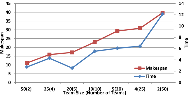
Figure 3: Results on 30$\times$30 4-neighbor grids with randomly blocked cells for different team sizes. ($K$ is the number of teams.)

For Experiment 2, there are 100 agents but the number of agents in a team (team size) varies from 50 to 2, resulting in $K=2\ldots 50$ teams. For each team size, we generate 50 TAPF instances as described before.

Table 3 shows the means of the makespans and running times (in seconds) over the instances that are solved within a time limit of 5 minutes each. CBM solves all TAPF instances within the time limit. For large team sizes and thus small numbers of teams, the makespans are small because CBM has more freedom to assign agents to targets. The running times are also small because the min-cost max-flow algorithm on the low level is fast even for large numbers of agents while CBS on the high level is fast because it needs to resolve collisions among agents in different teams but there are only a small number of teams. Thus, it is advantageous for teams to consist of as many agents as possible.

4.3 Experiment 3: Number of Agents

agts mkspn time success 100 30.10 6.14 1 150 29.67 8.10 0.96 200 32.09 12.97 0.94 250 31.05 15.56 0.86 300 32.09 25.42 0.7 350 33.03 32.59 0.6 400 34.19 59.69 0.42 450 35.80 101.47 0.1

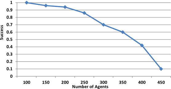
Figure 4: Results on 30$\times$30 4-neighbor grids with randomly blocked cells for different numbers of agents.

For Experiment 3, each team consists of 5 agents but the number of agents varies from 100 to 450, resulting in $20\ldots 90$ teams. For each number of agents, we generate 50 TAPF instances as described before.

Table 3 shows the success rates as well as the means of the makespans and running times (in seconds) over the instances that are solved within a time limit of 5 minutes each. For 250 agents or fewer, the success rate is larger than 85%. Current (non-anonymous) MAPF algorithm are not able to handle instances of this scale. As the number of agents increases, the success rates decrease and the makespans and running times increase due to the increasing number of collisions among agents in different teams produced by the min-cost max-flow algorithm on the low level. For 450 agents, for example, more than half of the unblocked cells are occupied by agents and thus many start cells of agents are also targets for other agents.

4.4 Experiment 4: Warehouse System

Figure 5: A randomly generated Kiva instance. CBM returns a solution with makespan 65 in 25.97 seconds. The length of the shortest path for both green drive units near the top-right corner to the green inventory station in the bottom-left corner is 64. Thus, at least one of them has to wait for at least one time step to enter the green inventory station and the solution found by CBM is optimal.

We now apply CBM to a simulated Kiva (now: Amazon Robotics) warehouse system kiva . Figure 1 shows a typical grid layout with inventory stations on the left side and storage locations in the storage area to the right of the inventory stations. Each inventory station has an entrance (purple cells) and an exit (pink cells). Each storage location (green cell) can store one inventory pod. Each inventory pod consists of a stack of trays, each of which holds bins with products. The autonomous warehouse robots are called drive units. Each drive unit is capable of picking up, carrying and putting down one inventory pod at a time. As a team, the drive units need to move inventory pods all the way from their storage locations to the inventory stations that need the products they store (to ship them to customers) and then back to the same or different empty storage locations. After a drive unit enters an inventory station, the requested product is removed from its inventory pod by a worker. Once drive units have delivered all requested products for one shipment to the same inventory station, the worker prepares the shipment to the customer.

Figure 5 shows a randomly generated Kiva instance. The light grey cells are free space. The dark grey cells are storage locations occupied by inventory pods and thus blocked. There are 7 inventory stations on the left side. The red cells are their exits, and the other 7 cells with graduated blue-green colors are their entrances. Drive units can enter and leave the inventory stations one at a time through their entrances and exits, respectively. The cells with graduated blue-green colors in the storage area are occupied by drive units. Each drive unit needs to carry the inventory pod in its current cell to the inventory station of the same color.

For Experiment 4, we generate 50 TAPF instances. Each instance has 420 drive units. 210 “incoming” drive units start at randomly determined storage locations: 30 drive units each need to move their inventory pods to the 7 inventory stations. In order to create difficult Kiva instances, we generate the start cells of these drive units randomly among all storage locations rather than cluster them according to their target inventory stations. 210 “outgoing” drive units start at the inventory stations: 30 drive units each need to move their inventory pods from the 7 inventory stations to the storage locations vacated by the incoming drive units. The task is to assign the 210 outgoing drive units to the vacated storage locations and plan collision-free paths for all 420 drive units in a way such that the makespan is minimized. The incoming drive units that have the same inventory station as target are a team (since they can arrive at the inventory station in any order), and all outgoing drive units are a team.

So far, we have assumed that, for any TAPF instance, all start vertices are unique, all targets are unique and each of the teams is given the same number of targets as there are agents in the team but these assumptions are not necessarily satisfied here. 1) The outgoing drive units that start at the same inventory station all start at its exit. In this case, we change the construction of the $T$-step time-extended network for the team of outgoing drive units so that there is a supply of one unit at vertex $v_{t}^{out}\in\mathcal{V^{\prime}}$ for all $t=0\ldots 29$ and all vertices $v\in V$ that correspond to exits of inventory stations. This construction forces the outgoing drive units that start at the same inventory station to leave it one after the other during the first 30 time steps. No further changes are necessary. 2) The incoming drive units that have the same inventory station as target all end at its entrance. In this case, we change the construction of the $T$-step time-extended network for each team of incoming drive units so that there is an auxiliary vertex with a demand of 30 units and vertex $v_{t}^{out}\in\mathcal{V^{\prime}}$ for all $t=0\ldots T$ is connected to the auxiliary vertex with an edge with unit capacity and zero edge weight, where $v\in V$ corresponds to the entrance of the inventory station. This construction forces the incoming drive units to enter the inventory station at different time steps. No further changes are necessary. 3) There could be more empty storage locations than outgoing drive units. In this case, no changes are necessary.

CBM finds solutions for 40 of the 50 Kiva instances within a time limit of 5 minutes each, yielding a success rate of 80%. The mean of the makespan over the solved Kiva instances is 63.73, and the mean of the running time is 91.61 seconds. Since early Kiva warehouse systems typically had about 200 drive units in more spacious (and thus less challenging) warehouses and even bounded-suboptimal (non-anonymous) MAPF algorithms that were specifically designed for simulated Kiva warehouse systems do not scale well to hundreds of agents DBLP:conf/socs/CohenUK15 , we conclude that CBM is a promising TAPF algorithm for applications of real-world scale.

5 Conclusions

In this paper, we studied the TAPF (combined target-assignment and path-finding) problem for teams of agents in known terrain to bridge the gap between the extreme cases of anonymous and non-anonymous MAPF problems, as required by many applications. We presented CBM, a hierarchical algorithm that is correct, complete and optimal for solving the TAPF problem. CBM outperforms (non-anonymous) MAPF algorithms in terms of both scalability and solution quality in our experiments. It also generalizes to applications with dozens of teams and hundreds of agents, which demonstrates its promise.

6 Acknowledgments

We thank Jingjin Yu for making the code of their ILP-based MAPF solver and Guni Sharon for making the code of their CBS solver available to us. Our research was supported by NASA via Stinger Ghaffarian Technologies as well as NSF under grant numbers 1409987 and 1319966 and a MURI under grant number N00014-09-1-1031. The views and conclusions contained in this document are those of the authors and should not be interpreted as representing the official policies, either expressed or implied, of the sponsoring organizations, agencies or the U.S. government.

References

- [1] J. E. Aronson. A survey of dynamic network flows. Annals of Operations Research, 20(1-4):1–66, 1989.
- [2] M. Barer, G. Sharon, R. Stern, and A. Felner. Suboptimal variants of the conflict-based search algorithm for the multi-agent pathfinding problem. In Annual Symposium on Combinatorial Search, pages 19–27, 2014.
- [3] E. Boyarski, A. Felner, R. Stern, G. Sharon, D. Tolpin, O. Betzalel, and S. E. Shimony. ICBS: improved conflict-based search algorithm for multi-agent pathfinding. In International Joint Conference on Artificial Intelligence, pages 740–746, 2015.
- [4] L. Cohen, T. Uras, and S. Koenig. Feasibility study: Using highways for bounded-suboptimal multi-agent path finding. In Annual Symposium on Combinatorial Search, pages 2–8, 2015.
- [5] B. de Wilde, A. W. ter Mors, and C. Witteveen. Push and rotate: Cooperative multi-agent path planning. In International Conference on Autonomous Agents and Multi-agent Systems, pages 87–94, 2013.
- [6] E. Erdem, D. G. Kisa, U. Oztok, and P. Schueller. A general formal framework for pathfinding problems with multiple agents. In AAAI Conference on Artificial Intelligence, pages 290–296, 2013.
- [7] A. V. Goldberg and R. E. Tarjan. Solving minimum-cost flow problems by successive approximation. In Annual ACM Symposium on Theory of Computing, pages 7–18, 1987.
- [8] M. Goldenberg, A. Felner, R. Stern, G. Sharon, N. R. Sturtevant, R. C. Holte, and J. Schaeffer. Enhanced partial expansion A*. Journal of Artificial Intelligence Research, 50:141–187, 2014.
- [9] R. Luna and K. E. Bekris. Push and swap: Fast cooperative path-finding with completeness guarantees. In International Joint Conference on Artificial Intelligence, pages 294–300, 2011.
- [10] H. Ma, C. Tovey, G. Sharon, T. K. S. Kumar, and S. Koenig. Multi-agent path finding with payload transfers and the package-exchange robot-routing problem. In AAAI Conference on Artificial Intelligence, 2016.
- [11] P. MacAlpine, E. Price, and P. Stone. SCRAM: Scalable collision-avoiding role assignment with minimal-makespan for formational positioning. In AAAI Conference on Artificial Intelligence, pages 2096–2102, 2015.
- [12] R. Morris, C. Pasareanu, K. Luckow, W. Malik, H. Ma, S. Kumar, and S. Koenig. Planning, scheduling and monitoring for airport surface operations. In AAAI-16 Workshop on Planning for Hybrid Systems, 2016.
- [13] G. Sharon, R. Stern, A. Felner, and N. R. Sturtevant. Conflict-based search for optimal multi-agent pathfinding. Artificial Intelligence, 219:40–66, 2015.
- [14] G. Sharon, R. Stern, M. Goldenberg, and A. Felner. The increasing cost tree search for optimal multi-agent pathfinding. Artificial Intelligence, 195:470–495, 2013.
- [15] D. Silver. Cooperative pathfinding. In Artificial Intelligence and Interactive Digital Entertainment, pages 117–122, 2005.
- [16] T. S. Standley. Finding optimal solutions to cooperative pathfinding problems. In AAAI Conference on Artificial Intelligence, pages 173–178, 2010.
- [17] P. Surynek. Reduced time-expansion graphs and goal decomposition for solving cooperative path finding sub-optimally. In International Joint Conference on Artificial Intelligence, pages 1916–1922, 2015.
- [18] C. Tovey, M. Lagoudakis, S. Jain, and S. Koenig. The Generation of Bidding Rules for Auction-Based Robot Coordination. In L. Parker, F. Schneider, and A. Schultz, editors, Multi-Robot Systems. From Swarms to Intelligent Automata, volume 3, chapter 1, pages 3–14. Springer, 2005.
- [19] M. Veloso, J. Biswas, B. Coltin, and S. Rosenthal. CoBots: Robust Symbiotic Autonomous Mobile Service Robots. In International Joint Conference on Artificial Intelligence, pages 4423–4429, 2015.
- [20] G. Wagner and H. Choset. Subdimensional expansion for multirobot path planning. Artificial Intelligence, 219:1–24, 2015.
- [21] G. Wagner, H. Choset, and N. Ayanian. Subdimensional expansion and optimal task reassignment. In Annual Symposium on Combinatorial Search, pages 177–178, 2012.
- [22] P. R. Wurman, R. D’Andrea, and M. Mountz. Coordinating hundreds of cooperative, autonomous vehicles in warehouses. AI Magazine, 29(1):9–20, 2008.
- [23] J. Yu and S. M. LaValle. Multi-agent path planning and network flow. In E. Frazzoli, T. Lozano-Perez, N. Roy, and D. Rus, editors, Algorithmic Foundations of Robotics X, Springer Tracts in Advanced Robotics, volume 86, pages 157–173. Springer, 2013.
- [24] J. Yu and S. M. LaValle. Planning optimal paths for multiple robots on graphs. In IEEE International Conference on Robotics and Automation, pages 3612–3617, 2013.
- [25] J. Yu and D. Rus. Pebble motion on graphs with rotations: Efficient feasibility tests and planning algorithms. In Algorithmic Foundations of Robotics XI, Springer Tracts in Advanced Robotics, volume 107, pages 729–746. Springer, 2015.
- [26] X. Zheng and S. Koenig. K-swaps: Cooperative negotiation for solving task-allocation problems. In International Joint Conference on Artifical Intelligence, pages 373–378, 2009.