Recent progress on intrinsic charm

Abstract

Over the past $\sim\!\!10$ years, the topic of the nucleon’s nonperturbative or intrinsic charm (IC) content has enjoyed something of a renaissance, largely motivated by theoretical developments involving quark modelers and PDF fitters. In this talk I will briefly describe the importance of intrinsic charm to various issues in high-energy phenomenology, and survey recent progress in constraining its overall normalization and contribution to the momentum sum rule of the nucleon. I end with the conclusion that progress on the side of calculation has now placed the onus on experiment to unambiguously resolve the proton’s intrinsic charm component.

1 Introduction

The nucleon’s nonperturbative (i.e., intrinsic) component has been a largely unresolved issue for the past several decades following the idea’s first incarnation in the seminal paper of Brodsky, Hoyer, Peterson, and Sakai (BHPS) BHPS , which I briefly review in Sec. 2.1 below. Despite this long history, the problem of incontrovertibly establishing the existence of intrinsic charm (IC) empirically and determining an overall numerical magnitude for its contribution to the proton wave function has been something of a Gordian knot. At the time of its proposal, the BHPS framework exploited recent developments in light-front field theory Chang-Yan ; Lepage to formulate a simple picture based upon a Fock-state expansion of the nucleon wave function to include $5$-quark states $|uudc\bar{c}\rangle$ involving charm not generated through the usual pQCD (or extrinsic) mechanism(s). Despite considerable variation, models of intrinsic charm (IC) unavoidably involve some expression of this fundamental idea, and in this talk I survey recent progress developing calculations of this sort, as well as numerical work to constrain the range of possibilities for the size of IC that has proceeded apace.

2 Modeling the proton’s intrinsic charm

Various theoretical approaches have proliferated in the past several decades, involving a number of assumed mechanisms for generating the intrinsic component of the charm PDF. Here I highlight several of these in increasing order of complexity.

2.1 Scalar frameworks

As the original scalar framework formulated in the infinite momentum frame (IMF), the above-mentioned BHPS description treats the transition probability for a proton with mass $M$ to go through a transition $p\to uudc\bar{c}$ (or, indirectly, to an internal $5$-quark state containing any heavy quark pair) in terms of an old-fashioned perturbation theory energy denominator expressible through the masses $m_{i}$ and momentum fractions $x_{i}$ of the constituents of the $5$-quark state,

$$P\Big{(}p\to uudc\bar{c}\Big{)}\ \sim\ \left[M^{2}-\sum_{i=1}^{5}\frac{m_{\perp i}^{2}}{x_{i}}\right]^{-2}.$$ (1)

In the expression above $x_{i}$ and $m_{\perp i}$ are, respectively, the light-front fraction and transverse mass of the $i^{th}$ quark, the latter explicitly given by $m_{\perp i}^{2}\equiv k_{\perp i}^{2}+m_{i}^{2}$, and the indices $4$ and $5$ are taken to apply to the heavy quark pair ($c$ and $\bar{c}$).

A special merit of this scheme is its simplicity: if one assumes the energy denominator of Eq. (1) to be controlled by the charm quark mass (i.e., $m^{2}_{c}=m^{2}_{\bar{c}}\gg m^{2}_{u/d},\ M^{2}$), the expression for the $5$-quark probability can be integrated to obtain a compact form for the the $x$ dependence of the IC PDF:

$$P(x)\ =\ \frac{Nx^{2}}{2}\left[\frac{(1-x)}{3}\left(1+10x+x^{2}\right)\ +\ 2x\,(1+x)\ln(x)\right],$$ (2)

in which I have taken $x_{5}\to x$, and the overall normalization $N$ is connected to the total intrinsic charm probability in the proton, subject to the constraint $\int dx\,c(x)=\int dx\,\bar{c}(x)$, which ensures the correct zero charm valence structure.

Building on the approach above, in a model-based analysis Pumplin1 of the nucleon’s heavy-quark content and subsequent QCD global fit Pumplin2 , Pumplin and (for the global analysis) collaborators considered a series of models for the Fock space wave function on the light-front for a proton to make a transition to a four quark plus one antiquark system, with the heavy $q\bar{q}$ pair composed of either charm or bottom quarks. This ansatz ultimately envisioned a simplified case wherein a spinless point particle of mass $m_{0}$ interacts with coupling strength $g$ to $N$ scalar particles having masses $m_{1},m_{2},\ldots,m_{N}$. Pumplin then found the unintegrated light-front probability density to have the form Pumplin1

$$dP\ =\ \frac{g^{2}}{(16\pi^{2})^{N-1}(N-2)!}\,\prod_{j=1}^{N}dx_{j}\,\delta\left(1-\sum_{j=1}^{N}x_{j}\right)\int_{s_{0}}^{\infty}ds\,\frac{(s-s_{0})^{N-2}}{(s-m_{0}^{2})^{2}}\,|F(s)|^{2},$$ (3)

where the invariant mass is $s_{0}=\sum_{j=1}^{N}m_{j}^{2}/x_{j}$, and a vertex function $F(s)$ must be stipulated to control behavior in the ultraviolet. In particular, if the transverse momenta and the factors of $1/x_{j}$ appearing in Eq. (3) are ignored and the charm mass is taken to be much larger than all other mass scales, one obtains the distribution prescribed by the BHPS model BHPS after also assuming a pointlike vertex factor $F(s)=1$. While these schemes are convenient and produce testable predictions for IC, a model with more physical interactions accounting for the structure of the charm spectrum is also desirable, and I sketch this idea in Sec. 2.2 now.

2.2 Meson-baryon models

As higher-mass extensions of the pion-cloud picture of nucleon structure, meson-baryon models (MBMs) are a natural framework for studying the proton’s interactions with external electromagnetic probes, relying on the advantageous properties of time-ordered perturbative theory (TOPT) and the convolution approach to compute corrections to the nucleon’s hadronic tensor, $W^{\mu\nu}$.

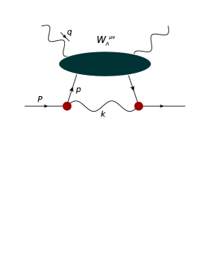
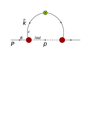
Figure 1: Diagrams relevant for the dominant contribution to the charm structure function in the MBM of Ref. Hobbs-IC . (Left) The TOPT diagram for the contribution of the dissociated $\Lambda_{c}D^{*}$ state to the hadronic tensor of the proton. (Right) An analogous diagram leading to the charm quark distribution within a spin-$1/2$ baryon (here, the $\Lambda_{c}$), $c_{B}(z)$, assuming a quark-diquark picture for the baryon’s constituent substructure; such processes are calculated in detail in Ref. Hobbs-IC .

Physically, a MBM describes the nucleon’s intrinsic charm content in a two-step ansatz formulated in terms of hadronic degrees of freedom as well as at quark level. Moreover, unlike the BHPS formalism with $m_{c}=m_{\bar{c}}$ in Sec. 2.1, MBMs can readily produce experimentally testable asymmetries between the $c$ and $\bar{c}$ distributions in the nucleon.

The basic goal of these models is the probability for the nucleon to spontaneously fluctuate into states involving an intermediate meson $M$ and baryon $B$, according to

$$|N\rangle\ =\ \sqrt{Z_{2}}\,\left|N\right.\rangle_{0}\ +\ \sum_{M,B}\int\!dy\,d^{2}\bm{k}_{\perp}\,\phi_{MB}(y,k^{2}_{\perp})\,\big{|}M(y,\bm{k}_{\perp});B(1-y,-\bm{k}_{\perp})\big{\rangle},$$ (4)

in which $\left|N\right.\rangle_{0}$ represents the undressed three-quark nucleon state, and $Z_{2}$ is an associated renormalization constant. The quantity $\phi_{MB}(y,k^{2}_{\perp})$ is an amplitude for the process whereby the nucleon reconfigures into an intermediate meson $M$ carrying a fraction $y$ of the proton’s longitudinal momentum and transverse momentum $\bm{k}_{\perp}$, and a baryon $B$ with longitudinal momentum fraction $1-y\equiv\bar{y}$ and transverse momentum $-\bm{k}_{\perp}$. The invariant mass squared $s_{MB}$ of this intermediate state appearing in the derivations below can then be expressed in the IMF by

$$s_{MB}(y,k^{2}_{\perp})\ =\ \frac{k^{2}_{\perp}+m_{M}^{2}}{y}+\frac{k^{2}_{\perp}+M_{B}^{2}}{1-y}\ \equiv\ s\,,$$ (5)

where the internal meson and baryon masses are respectively given by $m_{M}$ and $M_{B}$.

Ultimately, the dominant mechanism determining the IC distributions in the MBM of Ref. Hobbs-IC originated with the reconfiguration of the proton into intermediate states consisting of spin-$1$ charmed mesons $D^{*}=\bar{D}^{*0}$ or $D^{*-}$ and corresponding charm-containing baryons. The associated probabilistic splitting function for this mode is related to the amplitude of Eq. (4) by $f_{MB}(y)=\int_{0}^{\infty}d^{2}\bm{k}_{\perp}\,|\phi_{MB}(y,k^{2}_{\perp})|^{2}$, and, due to the higher $N$-$D^{*}$-$\Lambda_{c}$ spin interaction, arises from a linear combination of vector ($G_{v}$), tensor ($G_{t}$), and vector-tensor interference ($G_{vt}$) pieces. Viz.,

$$f_{D^{*}B}(y) =T_{B}\frac{1}{16\pi^{2}}\int{dk_{\perp}^{2}\over y(1-y)}{|F(s)|^{2}\over(s-M^{2})^{2}}\ \left[g^{2}\,G_{v}(y,k_{\perp}^{2})\ +\ {gf\over M}\,G_{vt}(y,k^{2}_{\perp})\ +\ \frac{f^{2}}{M^{2}}\,G_{t}(y,k^{2}_{\perp})\right]\ ,$$ (6)

where

$$G_{v}(y,k_{\perp}) =-6MM_{B}\ +\ \frac{4(P\cdot k)(p\cdot k)}{m_{D}^{2}}\ +\ 2P\cdot p\ ,$$ (7a)

$$G_{vt}(y,k_{\perp}) =4(M+M_{B})(P\cdot p-MM_{B})$$

$$-\ \frac{2}{m_{D}^{2}}\left[M_{B}(P\cdot k)^{2}-(M+M_{B})(P\cdot k)(p\cdot k)+M(p\cdot k)^{2}\right]\ ,$$ (7b)

$$G_{t}(y,k_{\perp}) =-(P\cdot p)^{2}\ +\ (M+M_{B})^{2}\,P\cdot p\ -\ MM_{B}(M^{2}+M_{B}^{2}+MM_{B})$$

$$+\ \frac{1}{2m_{D}^{2}}\Big{[}(P\cdot p-MM_{B})[(P-p)\cdot k]^{2}-2(M_{B}^{2}P\cdot k-M^{2}p\cdot k)[(P-p)\cdot k]$$

$$\hskip 28.45274pt+2(P\cdot k)(p\cdot k)(2P\cdot p-M_{B}^{2}-M^{2})\Big{]}\ ,$$ (7c)

and, as depicted in the left panel of Fig. 1, $p$ represents the $4$-momentum of the interacting baryon (e.g., $\Lambda^{+}_{c}$), $T_{B}$ is an isospin factor, and the products $P\cdot p$, $P\cdot k$, $p\cdot k$ can all be evaluated in terms of explicit TOPT expressions defined in the IMF as in the Appendices of Ref. Hobbs-IC . The hadronic interaction strengths $g$ and $f$ of Eq. (6) are fixed using SU$(4)$ quark model symmetry constraints á la standard Lippmann-Schwinger analyses Haiden .

A standard feature of this approach is the necessity of regulating the inevitable divergences that appear at large $k^{2}_{\perp}$ — a fact which follows from the essential status of MBMs as loop corrections or dressings to the photon-nucleon vertex. Typically, regularization is carried out phenomenologically, and implemented through a specific parametric choice for the relativistic vertex factor $F(s)$ appearing in Eq. (6), for example. The analysis of Ref. Hobbs-IC made use of a Gaussian with the form

$$F(s)=\exp[-(s-M^{2})/\Lambda^{2}]\ ,$$ (8)

in which $\Lambda$ is a cutoff parameter fixed across the various meson-baryon modes involved in the model and determined by fitting $pp\to\Lambda_{c}+X$ hadroproduction data from ISR ISR ; this yielded $\Lambda=(3.0\pm 0.2)$ GeV, leading to the predicted model bands plotted in Fig. 2 below.

Using this general formalism, one can compute other intermediate spin-isospin combinations for the possible charm-containing meson-baryon states of Eq. (4), and use an analogous framework embodied by the right panel of Fig. 1 to determine normalized distributions of (anti-)charm quarks within these hadronic states — e.g., the $c$ distribution within the $\Lambda_{c}$ meson, $c_{\Lambda}(z)$, as a function of a quark momentum fraction $z$. Having assembled these various ingredients, the MBM specifies the nonperturbative IC distribution at the partonic threshold $Q^{2}=m^{2}_{c}$ as an incoherent sum over various meson-baryon states:

$$\bar{c}(x)\ =\ \sum_{M,B}\,\Big{[}\int_{x}^{1}\frac{dy}{y}\,f_{MB}(y)\,\bar{c}_{M}\Big{(}\frac{x}{y}\Big{)}\ +\ \int_{x}^{1}\frac{d\bar{y}}{\bar{y}}\,f_{BM}(\bar{y})\,\bar{c}_{B}\Big{(}\frac{x}{\bar{y}}\Big{)}\Big{]}\ ,$$ (9a)

$$c(x)\ =\ \sum_{B,M}\,\Big{[}\int_{x}^{1}\frac{d\bar{y}}{\bar{y}}\,f_{BM}(\bar{y})\,c_{B}\Big{(}\frac{x}{\bar{y}}\Big{)}\ +\ \int_{x}^{1}\frac{dy}{y}\,f_{MB}(y)\,c_{M}\Big{(}\frac{x}{y}\Big{)}\Big{]}\ .$$ (9b)

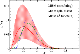
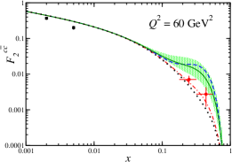
Figure 2: (Left) Intrinsic contributions to the proton’s charm PDF at the starting scale $Q^{2}_{0}=m^{2}_{c}$ of QCD evolution under different assumed prescriptions for the infrared behavior of the quark-hadron vertex that determines the distributions $\bar{c}_{M}(z)$ and $c_{B}(z)$. (Right) The charm sector part of the proton structure function $F^{c\bar{c}}_{2}=\big{(}4x\big{/}9\big{)}\left[c(x,Q^{2})+\bar{c}(x,Q^{2})\right]$ at an evolved scale of $Q^{2}=60$ GeV². The two red points belong to the highest EMC bin $\langle Q^{2}\rangle=60$ GeV² EMC ; while these points overhang the predictions of pQCD, they are at the lower periphery of the range predicted by the MBM informed by hadroproduction data.

The expressions in Eqs. (9a) and (9b) are the culmination of the MBM of Ref. Hobbs-IC and depend crucially upon assumed schemes to counter numerical poles in TOPT energy denominators that occur at infrared momenta in the quark-level amplitudes used to compute the distributions $\bar{c}_{M}(z)$ and $c_{B}(z)$. As described at length in Ref. Hobbs-IC , three main prescriptions were employed (a “confining” scheme to cancel the offending TOPT denominators, an “effective mass” approach in which the charm quark is taken to be sufficiently heavy as to avoid numerical poles, and a simple delta-function assumption for the quark distributions); after fixing UV regulators to hadroproduction data, starting-scale IC distributions such as those shown for $c(x)$ in the left panel of Fig. 2 were then obtained. For the sake of the data comparisons shown in the right panel of Fig. 2, these distributions were evolved according to pQCD to the empirical scale of the European Muon Collaboration (EMC) EMC , which measured the charm sector contribution to the $F_{2}(x,Q^{2})$ structure function of the proton via $\mu$-Fe DIS.

3 A QCD global analyses of the charm PDF

The model-based treatment of IC in Sec. 2.2 served the purpose of enlightening possible physical mechanisms for generating nonperturbative charm in a manner that led to direct constraints from experimental information. However, the ambiguity in the resulting magnitude of IC in the proton as suggested by the panels of Fig. 2 demanded a more systematic numerical approach. The most comprehensive such method involves performing a QCD global analysis of the world’s data explicitly including IC as a hypothesis. This was recently undertaken in Ref. GA-PRL using the $\mathcal{O}(\alpha_{s})$ formalism of Hoffmann and Moore HM for the charm structure function and, for the DGLAP starting-scale IC itself, the parametric shapes computed in the analysis of Ref. Hobbs-IC . In fact, in what follows the “confining” prescription corresponding to the central solid red curve in the LHS of Fig. 2 was used by default, and the commonly-used total momentum fraction was taken as a proxy for the overall normalization of IC in the proton:

$$\langle x\rangle_{\rm IC}\ \equiv\ \int_{0}^{1}dx\,x\left[c(x)+\bar{c}(x)\right]\ .$$ (10)

QCD global analyses of this quantity (as well as of an analogous fraction for intrinsic bottom Lyonnet:2015dca ) had been carried out by a number of groups over the years as exemplified by a recent CT14 calculation CT14 that assessed several IC scenarios (IC$=0$, as well as BHPS and a low $x$-dominated “sealike” shape); not unlike the earlier work of Ref. Pumplin2 , this determination found considerable levels of IC could be tolerated by a global fit — in particular, CT14 discovered that IC as large as $\langle x\rangle_{\rm IC}\sim 2-3\%$ could be accommodated within their framework, depending upon the specific IC scenario assumed.

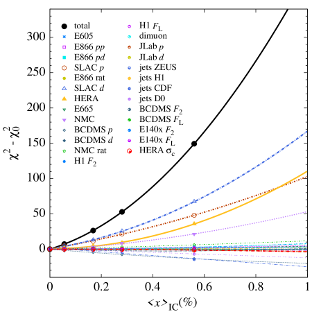
Figure 3: Aside from the EMC data which were not included in the global fit shown here, the full set of the JR14 analysis JR was first used to study the constraints imposed by the world’s data on the total IC fraction $\langle x\rangle_{\rm IC}$. As noted in TABLE I of Ref. JR and tabulated in the legend here, this involved 4296 data points from 26 independent sets of measurements. Moreover, the JR14 fitting technology incorporates a means of parametrizing the effects of dynamical higher twist, target mass, and nuclear corrections, enabling substantially less restrictive kinematical cuts: $Q^{2}\geq 1$ GeV² and $W^{2}\geq 3.5$ GeV². As a result, results were additionally constrained by important inputs from fixed-target SLAC data on proton and deuteron targets (brown circles and blue triangles, respectively), which drove the very rapid growth in the $\chi^{2}$ of the global fit relative to $\chi^{2}_{0}$ — the corresponding value at $\langle x\rangle_{\rm IC}=0$.

Unlike previous analyses, however, our recent effort in Ref. GA-PRL relied upon an updated formalism JR which accounted for various sub-leading $1/Q^{2}$ corrections (e.g., higher-twist effects and target mass corrections) and nuclear effects for DIS observables. This enhancement enabled a description of information at much lower $W^{2}$ and $Q^{2}$ than typically allowed in most global fits, and we therefore leveraged this to perform our QCD global analysis of IC with less restrictive kinematical cuts on the included data sets ($Q^{2}\geq 1$ GeV² and $W^{2}\geq 3.5$ GeV²). In Fig. 3, I summarize the contributions of the data sets included in the global analysis of Ref. GA-PRL to the total growth in the $\chi^{2}$ resulting from the fit. From the parabolas of Fig. 3, it is evident that some data sets (e.g., the H1 $F_{2}$ measurements corresponding to the blue-pentagon curve at bottom) do little to constrain $\langle x\rangle_{\rm IC}$; rather, the bulk of the constraint to the proton’s total IC (given by solid black disks) is driven by SLAC fixed-target information — on the deuteron (blue triangles) and proton (brown circles). The pronounced sensitivity of these data sets to IC can be interpreted as arising indirectly from the tightened constraints provided by the SLAC data to the light-quark sector of the global fit, which in turn limits the flexibility of the fitting framework in tolerating larger magnitudes for $\langle x\rangle_{\rm IC}$.

This point is further driven home by the left panel of Fig. 4, which separates the ‘SLAC’ contributions to the $\chi^{2}$ profile from the ‘rest’ of the data set summarized in Fig. 3. In the end, this global fit places quite stringent constraints on the magnitude of IC: $\langle x\rangle_{\rm IC}<0.1\%$ at the $5\sigma$ level.

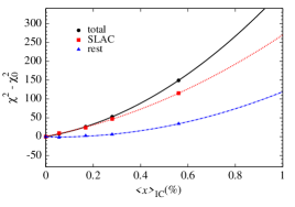
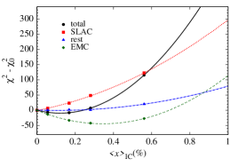
Figure 4: Plots of the $\chi^{2}$ growth profiles in the QCD global analysis of Ref. GA-PRL for runs in which EMC data were not included (left), and for global fits constrained by EMC (right).

An additional motivation for the analysis of Ref. GA-PRL , however, was the need to evaluate the suggestive measurements of EMC EMC . As has been pointed out numerous times in the literature, the highest $Q^{2}$ bins of the EMC data seem to provide some hint of the existence of IC, but before Ref. GA-PRL this information had not been treated in the context of a global analysis. Ultimately, incorporating the EMC points into the data set summarized in Fig. 3 led to a slight preference for nonzero IC, with the EMC set alone favoring $\langle x\rangle_{\rm IC}=0.3-0.4\%$ as indicated by the minimum in the green double-dotted curve on the RHS of Fig. 4. The modest preference for nonzero IC is diluted by the presence of other mitigating data sets, however, and the full global fit results in $\langle x\rangle_{\rm IC}=0.13\pm 0.04\%$ — a significantly reduced magnitude relative to the results of earlier analyses like Ref. CT14 . We also found the EMC points to be poorly fit (with $\chi^{2}/{\rm datum}=4.3$) and in some apparent tension with lower $Q^{2}$ points from HERA HERA . These issues necessitate further evaluation of the EMC set, and demand additional experimental measurement which might clarify the magnitude of IC without residual tension or ambiguity.

4 Recent developments in IC phenomenology

Following the completion of the work in Ref. GA-PRL , a number of intriguing developments in the phenomenology of IC have emerged, of which I highlight a couple of recent examples.

Partly motivated by the work of Refs. GA-PRL ; Reply , Ball et al. of the NNPDF Collaboration announced an independent global analysis NNPDF of the charm PDF in which the possibility of intrinsic charm was explicitly allowed via separate “Perturbative” and “Fitted” distributions which were then constrained through the neural networks-based methodology of NNPDF. Moreover, like Refs. GA-PRL ; Reply this work also incorporated the provocative EMC data, confronting them with a global fitting technology that does not presuppose a particular model-derived shape for the IC distribution; the relaxation of this aspect of typical QCD global fits affords the NNPDF framework greater flexibility in describing the world’s data, but can also result in distributions that are difficult to reconcile with the predictions of model-building. This fact is evident in the especially hard shape for the “Fitted” charm distribution obtained in Fig. 3 of Ref. NNPDF , which corresponded to $\langle x\rangle_{\rm IC}=0.7\pm 0.3\%$, and demands further study.

Aside from direct measurements of the charm structure function, more oblique means of accessing the nucleon’s nonperturbative charm content can be constructed. An archetypal example of this sort of approach can be found in the precise observation of prompt neutrino production Hallsie in dedicated cosmic-ray experiments like IceCube Laha . The analysis in this latter reference demonstrates that IC in accord with the upper reaches of the model predictions of Ref. Hobbs-IC (which allows larger IC normalizations and preceded the more systematic global analysis of Ref. GA-PRL ) might in principle be observable in the IceCube prompt neutrino spectrum; this suggest that such measurements could serve the role of an additional avenue to either observing or constraining the proton’s nonperturbative charm.

5 Conclusion and outlook

I have described the results of several closely related lines of investigation into the intrinsic charm problem. Given that direct experimental information is relatively limited, much of this work has been constrained in its ability to recommend a robust value for, e.g., the total IC momentum fraction $\langle x\rangle_{\rm IC}$. The present situation therefore seems to be one in which the reach of modeling and analyses of data is approaching a point of diminishing return, and additional empirical inputs would be invaluable. For this purpose modern, direct measurements of $F^{c\bar{c}}_{2}(x,Q^{2})$ — especially at large $x$ and low/intermediate $Q^{2}$ along the lines of the original EMC data — could better constrain both models and global analyses and settle some of the questions related to the interpretation of the EMC set itself as raised in Refs. GA-PRL ; Reply . Measurements of this type might ideally be carried out at a future electron-ion collider EIC and be complemented by work at the proposed AFTER@CERN fixed-target $pp$ experiment AFTER , which would putatively operate at $\sqrt{s}=115$ GeV; this might similarly be the case for a suggested measurement of the forward production of $Z$ bosons in coincidence with charm-containing jets at LHCb Williams , possibly exposing the behavior of the charm PDF in the critical valence region.

6 Acknowledgements

I thank Wally Melnitchouk, Tim Londergan, and Pedro Jimenez-Delgado for discussions and collaboration on various portions of this work. For additional useful conversations, I thank Stan Brodsky, Ranjan Laha, Gerald Miller, and Jean-Phillipe Lansberg. This work was supported by the U.S. Department of Energy Office of Science, Office of Basic Energy Sciences program under Award Number DE-FG02-97ER-41014.

References

- (1) S.J. Brodsky, P. Hoyer, C. Peterson, N. Sakai, Phys. Lett. B93, 451 (1980)
- (2) S.J. Chang, R.G. Root, T.M. Yan, Phys. Rev. D7, 1133 (1973)
- (3) G.P. Lepage, S.J. Brodsky, Phys. Rev. D22, 2157 (1980)
- (4) J. Pumplin, Phys. Rev. D73, 114015 (2006), hep-ph/0508184
- (5) J. Pumplin, H.L. Lai, W.K. Tung, Phys. Rev. D75, 054029 (2007), hep-ph/0701220
- (6) T.J. Hobbs, J.T. Londergan, W. Melnitchouk, Phys. Rev. D89, 074008 (2014), 1311.1578
- (7) J. Haidenbauer, G. Krein, U.G. Meissner, L. Tolos, Eur. Phys. J. A47, 18 (2011), 1008.3794
- (8) P. Chauvat et al. (R608), Phys. Lett. B199, 304 (1987)
- (9) J.J. Aubert et al. (European Muon), Nucl. Phys. B213, 31 (1983)
- (10) P. Jimenez-Delgado, T.J. Hobbs, J.T. Londergan, W. Melnitchouk, Phys. Rev. Lett. 114, 082002 (2015), 1408.1708
- (11) E. Hoffmann, R. Moore, Z. Phys. C20, 71 (1983)
- (12) F. Lyonnet, A. Kusina, T. JeÅo, K. KovarÃk, F. Olness, I. Schienbein, J.Y. Yu, JHEP 07, 141 (2015), 1504.05156
- (13) S. Dulat, T.J. Hou, J. Gao, J. Huston, J. Pumplin, C. Schmidt, D. Stump, C.P. Yuan, Phys. Rev. D89, 073004 (2014), 1309.0025
- (14) P. Jimenez-Delgado, E. Reya, Phys. Rev. D89, 074049 (2014), 1403.1852
- (15) H. Abramowicz et al. (ZEUS, H1), Eur. Phys. J. C73, 2311 (2013), 1211.1182
- (16) P. Jimenez-Delgado, T.J. Hobbs, J.T. Londergan, W. Melnitchouk, Phys. Rev. Lett. 116, 019102 (2016), 1504.06304
- (17) R.D. Ball, V. Bertone, M. Bonvini, S. Carrazza, S. Forte, A. Guffanti, N.P. Hartland, J. Rojo, L. Rottoli (NNPDF) (2016), 1605.06515
- (18) R. Enberg, M.H. Reno, I. Sarcevic, Phys. Rev. D78, 043005 (2008), 0806.0418
- (19) R. Laha, S.J. Brodsky (2016), 1607.08240
- (20) A. Accardi et al., Eur. Phys. J. A52, 268 (2016), 1212.1701
- (21) S.J. Brodsky, A. Kusina, F. Lyonnet, I. Schienbein, H. Spiesberger, R. Vogt, Adv. High Energy Phys. 2015, 231547 (2015), 1504.06287
- (22) T. Boettcher, P. Ilten, M. Williams, Phys. Rev. D93, 074008 (2016), 1512.06666