Canonical Duality Theory for Topology Optimization

Abstract

This paper presents a canonical duality approach for solving a general topology optimization problem of nonlinear elastic structures. By using finite element method, this most challenging problem can be formulated as a mixed integer nonlinear programming problem (MINLP), i.e. for a given deformation, the first-level optimization is a typical linear constrained 0-1 programming problem, while for a given structure, the second-level optimization is a general nonlinear continuous minimization problem in computational nonlinear elasticity. It is discovered that for linear elastic structures, first-level optimization is a typical Knapsack problem, which is considered to be NP-complete in computer science. However, by using canonical duality theory, this well-known problem can be solved analytically to obtain exact integer solution. A perturbed canonical dual algorithm (CDT) is proposed and illustrated by benchmark problems in topology optimization. Numerical results show that the proposed CDT method produces desired optimal structure without any gray elements. The checkerboard issue in traditional methods is much reduced.

1 General Topology Optimization Problem and Challenges

Topology optimization aims to distribute materials within a prescribed design domain in order to obtain the best structural performance under certain geometric or physical constraints. Due to its broad applications, the topology optimization has been subjected to extensively study since the seminal paper by Bendsoe and Kikuch bb_Bendsoe88 . Generally speaking, a typical topology optimization problem involves both continuous state variable and discrete density distribution that can take either the value 0 (void) or 1 (solid material) at any point in the design domain. Thus, numerical discretization methods (say FEM) for solving topology optimization problems lead to a so-called mixed integer nonlinear programming (MINLP) problem, which appears extensively in computational engineering, decision and management sciences, operations research, industrial and systems engineering gao-aip16 .

Let us consider an elastically deformable body that in an undeformed configuration occupies an open domain $\Omega\subset\mathbb{R}^{d}\;(d=2,3)$ with (Lipschitz) boundary $\Gamma=\partial\Omega$. We assume that the body is subjected to a body force ${\bf f}$ (per unit mass) in the reference domain $\Omega$ and a given surface traction $\mathbf{t}(\mathbf{x})$ of dead-load type on the boundary ${\Gamma_{t}}\subset\partial\Omega$, while the body is fixed on the remaining boundary ${\Gamma_{u}}=\partial\Omega\cap{\Gamma_{t}}$. Based on the minimal potential principle in continuum mechanics, the topology optimization of compliance minimization problem of this elastic body can be formulated in the following coupled minimization problem

$$({\cal P}):\;\;\min_{\mathbf{u}\in{\cal U}_{a}}\min_{\rho\in{\cal Z}}\left\{\Pi(\mathbf{u},\rho)=\int_{\Omega}W(\nabla\mathbf{u})\rho{\rm d}\Omega+\int_{\Omega}\mathbf{u}\cdot{\bf f}\rho{\rm d}\Omega-\int_{\Gamma_{t}}\mathbf{u}\cdot\mathbf{t}{\rm d}\Gamma\right\},$$ (1)

where the unknown $\mathbf{u}:\Omega\rightarrow\mathbb{R}^{d}$ is a displacement vector field, the design variable $\rho(\mathbf{x})\in\{0,1\}$ is a discrete scalar field, the stored energy per unit reference volume $W(\mathbf{D})$ is a nonlinear differentiable function of the deformation gradient $\mathbf{D}=\nabla\mathbf{u}$. The notation ${\cal U}_{a}$ identifies a kinematically admissible space of deformations, in which, certain geometrical/boundary conditions are given, and

$${\cal Z}=\left\{\rho(\mathbf{x}):\Omega\rightarrow\{0,1\}|\;\;\int_{\Omega}\rho(\mathbf{x}){{\rm d}\Omega}\leq V_{c}\right\}$$

is a design feasible space, in which, $V_{c}>0$ is the desired volume.

Mathematically speaking, the topology optimization $({\cal P})$ is a coupled nonlinear-discrete minimization problem in infinite-dimensional space. For large deformation problems, the stored energy $W(\mathbf{D})$ is usually nonconvex. The criticality condition of this minimization problem leads to a nonlinear system of highly coupled partial differential equations. It is fundamentally difficult to analytically solve this type of problems. Numerical methods must be adopted.

Finite element method is the most popular numerical approach for topology optimization, by which, the domain $\Omega$ is divided into $n$ disjointed elements $\{\Omega_{e}\}$ and in each element, the unknown fields can be numerically discretized as

$$\mathbf{u}(\mathbf{x})=\mathbf{N}_{e}(\mathbf{x})\mathbf{u}_{e},\;\;\rho(\mathbf{x})=\rho_{e}\in\{0,1\}\;\;\forall\mathbf{x}\in\Omega_{e},$$ (2)

where $\mathbf{N}_{e}$ is an interpolation matrix, $\mathbf{u}_{e}$ is a nodal displacement vector, the binary design variable $\rho_{e}\in\{0,1\}$ is used for determining whether the element $\Omega_{e}$ is a void ($\rho_{e}=0$) or a solid ($\rho_{e}=1$). Thus, by substituting (2) into $\Pi(\mathbf{u},\rho)$ and let ${\cal U}^{m}_{a}\subset\mathbb{R}^{m}$ be an admissible nodal displacement space,

$${\cal Z}_{a}=\left\{\mbox{\boldmath$\rho$}=\{\rho_{e}\}\in\{0,1\}^{n}|\;\;V(\mbox{\boldmath$\rho$})=\sum_{e=1}^{n}\rho_{e}\Omega_{e}\leq V_{c}\right\},$$ (3)

the variational problem $({\cal P})$ can be numerically reformulated the following global optimization problem

$$({\cal P}_{h}):\;\;\;\min_{\mathbf{u}\in{\cal U}^{m}_{a}}\min_{\mbox{\boldmath$\rho$}\in{\cal Z}_{a}}\left\{\Pi_{h}(\mathbf{u},\mbox{\boldmath$\rho$})=C(\mbox{\boldmath$\rho$},\mathbf{u})-\mathbf{u}^{T}\mathbf{f}(\mbox{\boldmath$\rho$})\right\},$$ (4)

where

$$C(\mbox{\boldmath$\rho$},\mathbf{u})=\mbox{\boldmath$\rho$}^{T}\mathbf{c}(\mathbf{u}),\;\;\mathbf{c}(\mathbf{u})=\left\{\int_{\Omega_{e}}W(\nabla\mathbf{N}(\mathbf{x})\mathbf{u}_{e}){{\rm d}\Omega}\right\}\in\mathbb{R}^{n},$$ (5)

$$\mathbf{f}(\mbox{\boldmath$\rho$})=\left\{\int_{\Omega_{e}}\rho_{e}\mathbf{N}_{e}(\mathbf{x})^{T}\mathbf{b}_{e}(\mathbf{x}){{\rm d}\Omega}\right\}+\left\{\int_{\Gamma^{e}_{t}}\mathbf{N}(\mathbf{x})^{T}\mathbf{t}(\mathbf{x}){{\rm d}\Gamma}\right\}\;\in\mathbb{R}^{m}.$$ (6)

Clearly, this discretized topology optimization involves both the continuous variable $\mathbf{u}\in{\cal U}^{m}_{a}$ and the integer variable $\mbox{\boldmath$\rho$}\in{\cal Z}_{a}$, it is the so-called mixed integer nonlinear programming problem (MINLP) in mathematical programming. Since $\rho_{e}^{p}=\rho_{e}\;\;\forall\rho_{e}\in\{0,1\},\;\;\forall p\in\mathbb{R},$ we have

$$C_{p}(\mbox{\boldmath$\rho$},\mathbf{u}):=\sum_{e=1}^{n}\rho_{e}^{p}c_{e}(\mathbf{u})=(\;\underbrace{\mbox{\boldmath$\rho$}\circ\dots\circ\mbox{\boldmath$\rho$}}_{p\mbox{ times }}\;)^{T}\mathbf{c}(\mathbf{u})=C(\mbox{\boldmath$\rho$},\mathbf{u})\;\;\;\forall p\in\mathbb{R},$$ (7)

where $\mbox{\boldmath$\rho$}\circ\mathbf{c}=\{\rho_{e}c_{e}\}$ represents the Hadamard product. Particularly, for $p=2$, we write

$$C_{2}(\mbox{\boldmath$\rho$},\mathbf{u}):=\frac{1}{2}\mbox{\boldmath$\rho$}^{T}\mathbf{A}(\mathbf{u})\mbox{\boldmath$\rho$},\;\;\;\mathbf{A}(\mathbf{u})=2\mbox{Diag}\{\mathbf{c}(\mathbf{u})\}.$$ (8)

Clearly, $C_{2}(\mbox{\boldmath$\rho$},\mathbf{u})$ is a convex function of $\rho$ since $\mathbf{A}(\mathbf{u})\succeq 0\;\;\forall\mathbf{u}\in{\cal U}^{m}_{a}$. By the facts that $\mbox{\boldmath$\rho$}\in{\cal Z}_{a}$ is the main design variable and the displacement $\mathbf{u}$ depends on each given domain $\Omega$, the problem $({\cal P}_{h})$ is actually a so-called bi-level programming problem:

$$({\cal P}_{bl}):\;\; \min_{\mbox{\boldmath$\rho$}\in{\cal Z}_{a}}\min_{\mathbf{u}\in{\cal U}^{m}_{a}}\{C_{p}(\mbox{\boldmath$\rho$},\mathbf{u})-\mathbf{u}^{T}\mathbf{f}(\mbox{\boldmath$\rho$})\}$$ (9)

$$s.t. \mathbf{u}=\arg\min_{\mathbf{v}\in{\cal U}^{m}_{a}}\Pi_{h}(\mathbf{v},\mbox{\boldmath$\rho$}).$$ (10)

In this formulation, $C_{p}(\mbox{\boldmath$\rho$},\mathbf{u})-\mathbf{u}^{T}\mathbf{f}(\mbox{\boldmath$\rho$})$ represents the upper-level cost function and the total potential energy $\Pi_{h}(\mathbf{u},\mbox{\boldmath$\rho$})$ represents the lower-level cost function. For large deformation problems, the total potential energy $\Pi_{h}$ is usually a nonconvex function of $\mathbf{u}$. Therefore, this bi-level optimization could be the most challenging problem in global optimization.

For linear elastic structures, the total potential energy $\Pi_{h}$ is a quadratic function of $\mathbf{u}$

$$\Pi_{h}(\mathbf{u},\mbox{\boldmath$\rho$})=\frac{1}{2}\mathbf{u}^{T}\mathbf{K}(\mbox{\boldmath$\rho$})\mathbf{u}-\mathbf{u}^{T}\mathbf{f}(\mbox{\boldmath$\rho$})$$ (11)

where $\mathbf{K}(\mbox{\boldmath$\rho$})=\left\{\rho_{e}\mathbf{K}_{e}\right\}\in\mathbb{R}^{m\times m}$ is the overall stiffness matrix, which is obtained by assembling the sub-matrix $\rho_{e}\mathbf{K}_{e}$ for each element $\Omega_{e}$. In this case, the lower-level optimization (10) is a convex minimization and for each given upper-level design variable $\rho$, the lower-level solution is simply governed by the linear equilibrium equation $\mathbf{K}(\mbox{\boldmath$\rho$})\mathbf{u}=\mathbf{f}(\mbox{\boldmath$\rho$}).$ Therefore, the topology optimization for linear elasticity is mathematically an linear constrained integer programming problem:

$$({\cal P}_{le}):\;\;\min_{\mbox{\boldmath$\rho$}\in{\cal Z}_{a}}\min_{\mathbf{u}\in{\cal U}^{m}_{a}}\left\{-\frac{1}{2}\mathbf{u}^{T}\mathbf{K}(\mbox{\boldmath$\rho$})\mathbf{u}|\;\;\;\mathbf{K}(\mbox{\boldmath$\rho$})\mathbf{u}=\mathbf{f}(\mbox{\boldmath$\rho$})\right\}.$$ (12)

Due to the integer constraint, to solve this mixed integer quadratic minimization problem is fundamentally difficult. In order to overcome the combinatorics complexity in this problem, various approximations were proposed during the last decades, including homogenization bb_Bendsoe88 , density-based approximations bb_Bendsoe89 , level set method bb_VanDijk2013 , and topological derivative bb_Sokolowski99 , etc . These approaches generally relax the MINLP problem into a continuous parameter optimization problem by using size, density or shape, and then solve it based on the traditional Newton-type (gradient-based) or evolutionary optimization algorithms. A comprehensive survey on these approaches was given in bb_Sigmund2013 .

The so-called Simplified Isotropic Material with Penalization (SIMP) is one of the most popular approaches in topology optimization:

$$(SIMP):\;\; \min_{\mbox{\boldmath$\rho$}\in\mathbb{R}^{N}}C_{p}(\mbox{\boldmath$\rho$},\mathbf{u}(\mbox{\boldmath$\rho$}))$$ (13)

$$s.t. \;\;\mathbf{K}(\mbox{\boldmath$\rho$}^{p})\mathbf{u}=\mathbf{f}(\mbox{\boldmath$\rho$}),\;\;V(\mbox{\boldmath$\rho$})\leq V_{c},$$ (15)

$$\;\;0<\rho_{e}\leq 1,\ e=1,\ldots,n$$

where $p$ is the so-called penalization parameter in topology optimization. The SIMP formulation has been studied extensively in topology optimization and numerous research papers have been produced during the past decades. By the fact that $\mbox{\boldmath$\rho$}^{p}=\mbox{\boldmath$\rho$}\;\;\forall p\in\mathbb{R},\;\;\forall\mbox{\boldmath$\rho$}\in\{0,1\}^{n}$, we can see that the integer constraint $\mbox{\boldmath$\rho$}\in\{0,1\}^{n}$ in $({\cal P}_{le})$ is simply replaced by the box constraint $\mbox{\boldmath$\rho$}\in(0,1]^{n}$. Although it was discovered by engineers that the “magic number” $p=3$ can ensure good convergence to almost $0$-$1$ solutions, the SIMP formulation is not mathematically equivalent to the topology optimization problem $({\cal P}_{le})$. Actually, in many real-world applications, most SIMP solutions $\{\rho_{e}\}$ are only approximate to $0$ or $1$ but never be exactly $0$ or $1$. Correspondingly, these elements are in gray scale which have to be filtered or interpreted physically. Additionally, this method suffers some key limitations such as the unsure global optimization, many gray scale elements and checkerboard patterns, etc.

2 Canonical Dual Problem and Analytical Solution

Canonical dual finite element methods for solving elasto-plastic structures and large deformation problems have been studied since 1988 gao-cs88 ; gao-jem96 . Applications to nonconvex mechanics are given recently for post-buckling problems ali-gao ; santos-gao . This paper will address the canonical duality theory for solving the challenging integer programming problem in $({\cal P}_{u})$.

Let $\mathbf{a}=\{a_{e}=\mbox{Vol}(\Omega_{e})\}\in\mathbb{R}^{n}$, where $\mbox{Vol}(\Omega_{e})$ represents the volume of each element $\Omega_{e}$. Then we have ${\cal Z}_{a}=\{\mbox{\boldmath$\rho$}\in\{0,1\}^{n}|\;\;\mbox{\boldmath$\rho$}^{T}\mathbf{a}\leq V_{c}\}$. By the fact that $\min_{\mbox{\boldmath$\rho$}}\min_{\mathbf{u}}=\min_{\mathbf{u}}\min_{\mbox{\boldmath$\rho$}}$, the alternative iteration can be adopted for solving the topology optimization problem. Since $C_{1}(\mbox{\boldmath$\rho$},\mathbf{u})=\frac{1}{2}\mathbf{u}^{T}\mathbf{K}(\mbox{\boldmath$\rho$})\mathbf{u}=\mbox{\boldmath$\rho$}^{T}\mathbf{c}(\mathbf{u})$, for a given solution of (10), the energy vector $\mathbf{c}_{u}=\mathbf{c}(\mathbf{u})\in\mathbb{R}^{n}_{+}$ is non-negative. Thus, the iterative method for linear elastic topology optimization $({\cal P}_{le})$ can be proposed for solving the following linear 0-1 programming problem ($({\cal P})$ for short) :

$$({\cal P}):\;\;\min\left\{P_{u}(\mbox{\boldmath$\rho$})=-\mathbf{c}_{u}^{T}\mbox{\boldmath$\rho$}\;\;|\;\;\mbox{\boldmath$\rho$}\in\{0,1\}^{n},\;\;\mbox{\boldmath$\rho$}^{T}\mathbf{a}\leq V_{c}\right\}.$$ (16)

This is the well-known Knapsack problem. Due to the 0-1 constraint, even this most simple linear integer programming is listed as one of Karp’s 21 NP-complete problems karp . However, this challenging problem can be solved analytically by using the canonical duality theory.

The canonical duality theory for general integer programming was first proposed by Gao in 2007 gao-jimo07 . The key idea of this theory is the introducing of a canonical measure

$$\mbox{\boldmath$\xi$}=\Lambda(\mbox{\boldmath$\rho$})=\{\mbox{\boldmath$\rho$}\circ\mbox{\boldmath$\rho$}-\mbox{\boldmath$\rho$},\;\;\mbox{\boldmath$\rho$}^{T}\mathbf{a}-V_{c}\}:\;\;\mathbb{R}^{n}\rightarrow{\cal E}=\mathbb{R}^{n+1}.$$ (17)

Let

$${\cal E}_{a}:=\{\mbox{\boldmath$\xi$}=\{\mbox{\boldmath$\epsilon$},\nu\}\in\mathbb{R}^{n+1}|\;\;\mbox{\boldmath$\epsilon$}\leq 0,\;\;\nu\leq 0\}$$ (18)

be a convex cone in $\mathbb{R}^{n+1}$. Its indicator $\Psi(\mbox{\boldmath$\xi$})$ is defined by

$$\Psi(\mbox{\boldmath$\xi$})=\left\{\begin{array}[]{ll}0&\mbox{ if }\mbox{\boldmath$\xi$}\in{\cal E}_{a}\\ +\infty&\mbox{ otherwise}\end{array}\right.$$

which is a convex and lower semi-continuous (l.s.c) function in $\mathbb{R}^{n+1}$. By this function, the primal problem can be relaxed in the following unconstrained minimization form:

$$\min\left\{\Phi(\mbox{\boldmath$\rho$})=P_{u}(\mbox{\boldmath$\rho$})+\Psi(\Lambda(\mbox{\boldmath$\rho$}))\;\;|\;\;\mbox{\boldmath$\rho$}\in\mathbb{R}^{n}\right\}.$$ (19)

Due to the convexity of $\Psi(\mbox{\boldmath$\xi$})$, its conjugate function can be defined uniquely by the Fenchel transformation:

$$\Psi^{*}(\mbox{\boldmath$\zeta$})=\sup_{\mbox{\boldmath$\xi$}\in\mathbb{R}^{n+1}}\{\mbox{\boldmath$\xi$}^{T}\mbox{\boldmath$\zeta$}-\Psi(\mbox{\boldmath$\xi$})\}=\left\{\begin{array}[]{ll}0&\mbox{ if }\mbox{\boldmath$\zeta$}\in{\cal E}_{a}^{*}\\ +\infty&\mbox{ otherwise}\end{array}\right.$$ (20)

where ${\cal E}_{a}^{*}=\{\mbox{\boldmath$\zeta$}=\{\mbox{\boldmath$\sigma$},\varsigma\}\in\mathbb{R}^{n+1}|\;\;\mbox{\boldmath$\sigma$}\geq 0,\;\;\varsigma\geq 0\}$ is the dual space of ${\cal E}_{a}$. Thus, by using the Fenchel-Young equality $\Psi(\mbox{\boldmath$\xi$})+\Psi^{*}(\mbox{\boldmath$\zeta$})=\mbox{\boldmath$\xi$}^{T}\mbox{\boldmath$\zeta$}$, the function $\Phi(\mbox{\boldmath$\rho$})$ can be written in the Gao-Strang total complementary function gs-89

$$\Xi(\mbox{\boldmath$\rho$},\mbox{\boldmath$\zeta$})=P_{u}(\mbox{\boldmath$\rho$})+\Lambda(\mbox{\boldmath$\rho$})^{T}\mbox{\boldmath$\zeta$}-\Psi^{*}(\mbox{\boldmath$\zeta$}).$$ (21)

Based on this function, the canonical dual of $\Phi(\mbox{\boldmath$\rho$})$ can be defined by

$$\Phi^{d}(\mbox{\boldmath$\zeta$})=\mbox{sta }\{\Xi(\mbox{\boldmath$\rho$},\mbox{\boldmath$\zeta$})|\;\;\mbox{\boldmath$\rho$}\in\mathbb{R}^{m}\}=P^{\Lambda}_{u}(\mbox{\boldmath$\zeta$})-\Psi^{*}(\mbox{\boldmath$\zeta$})$$ (22)

where $\mbox{sta }\{f(x)|\;x\in X\}$ stands for finding a stationary value of $f(x)\;\;\forall x\in X$, and

$$P^{\Lambda}_{u}(\mbox{\boldmath$\zeta$})=\mbox{sta }\{\Lambda(\mbox{\boldmath$\rho$})^{T}\mbox{\boldmath$\zeta$}+P_{u}(\mbox{\boldmath$\rho$})\}=-\frac{1}{4}\mbox{\boldmath$\tau$}_{u}^{T}(\mbox{\boldmath$\zeta$})\mathbf{G}^{-1}(\mbox{\boldmath$\zeta$})\mbox{\boldmath$\tau$}_{u}(\mbox{\boldmath$\zeta$})-\varsigma V_{c}$$ (23)

is the $\Lambda$-conjugate of $P_{u}(\mbox{\boldmath$\rho$})$, in which,

$$\mathbf{G}(\mbox{\boldmath$\zeta$})=\ \mbox{Diag}\{\mbox{\boldmath$\sigma$}\},\;\;\;\mbox{\boldmath$\tau$}_{u}(\mbox{\boldmath$\zeta$})=\mbox{\boldmath$\sigma$}-\varsigma\mathbf{a}+\mathbf{c}_{u}.$$

Clearly, $P_{u}^{\Lambda}(\mbox{\boldmath$\zeta$})$ is well-defined if $\det\mathbf{G}\neq 0$, i.e. $\mbox{\boldmath$\sigma$}\neq 0\in\mathbb{R}^{n}$. Let ${\cal S}_{a}=\{\mbox{\boldmath$\zeta$}\in{\cal E}^{*}_{a}|\;\;\det\mathbf{G}\neq 0\}$. We have the following standard result in the canonical duality theory:

Theorem 2.1 (Complementary-Dual Principle)

For a given $\mathbf{u}\in{\cal U}^{m}_{a}$, if $(\bar{\mbox{\boldmath$\rho$}},\bar{\mbox{\boldmath$\zeta$}})$ is a KKT point of $\Xi$, then $\bar{\mbox{\boldmath$\rho$}}$ is a KKT point of $\Phi$, $\bar{\mbox{\boldmath$\zeta$}}$ is a KKT point of $\Phi^{d}$, and

$$\Phi(\bar{\mbox{\boldmath$\rho$}})=\Xi(\bar{\mbox{\boldmath$\rho$}},\bar{\mbox{\boldmath$\zeta$}})=\Phi^{d}(\bar{\mbox{\boldmath$\zeta$}}).$$ (24)

Proof

By the convexity of $\Psi(\mbox{\boldmath$\xi$})$, we have the following canonical duality relations:

$$\mbox{\boldmath$\zeta$}\in\partial\Psi(\mbox{\boldmath$\xi$})\;\;\Leftrightarrow\;\;\mbox{\boldmath$\xi$}\in\partial\Psi^{*}(\mbox{\boldmath$\zeta$})\;\;\Leftrightarrow\;\;\Psi(\mbox{\boldmath$\xi$})+\Psi^{*}(\mbox{\boldmath$\zeta$})=\mbox{\boldmath$\xi$}^{T}\mbox{\boldmath$\zeta$},$$ (25)

where

$$\partial\Psi(\mbox{\boldmath$\xi$})=\left\{\begin{array}[]{ll}\mbox{\boldmath$\zeta$}&\mbox{ if }\mbox{\boldmath$\xi$}\in{\cal E}_{a}\\ \emptyset&\mbox{ otherwise}\end{array}\right.$$

is the sub-differential of $\Psi$. Thus, in terms of $\mbox{\boldmath$\xi$}=\Lambda(\mbox{\boldmath$\rho$})$ and $\mbox{\boldmath$\zeta$}=\{\mbox{\boldmath$\sigma$},\varsigma\}$, the canonical duality relations (25) can be equivalently written as

$$\mbox{\boldmath$\rho$}\circ\mbox{\boldmath$\rho$}-\mbox{\boldmath$\rho$}\leq 0\;\;\Leftrightarrow\;\;\mbox{\boldmath$\sigma$}\geq 0\;\;\Leftrightarrow\;\;\mbox{\boldmath$\sigma$}^{T}(\mbox{\boldmath$\rho$}\circ\mbox{\boldmath$\rho$}-\mbox{\boldmath$\rho$})=0\;\;$$ (26)

$$\mbox{\boldmath$\rho$}^{T}\mathbf{a}-V_{c}\leq 0\;\;\Leftrightarrow\;\;\varsigma\geq 0\;\;\Leftrightarrow\;\;\varsigma(\mbox{\boldmath$\rho$}^{T}\mathbf{a}-V_{c})=0.$$ (27)

These are exactly the KKT conditions for the inequality constraints $\mbox{\boldmath$\rho$}\circ\mbox{\boldmath$\rho$}-\mbox{\boldmath$\rho$}\leq 0$ and $\mbox{\boldmath$\rho$}^{T}\mathbf{a}-V_{c}\leq 0$. Thus, $(\bar{\mbox{\boldmath$\rho$}},\bar{\mbox{\boldmath$\zeta$}})$ is a KKT point of $\Xi$ if and only if $\bar{\mbox{\boldmath$\rho$}}$ is a KKT point of $\Phi$, $\bar{\mbox{\boldmath$\zeta$}}$ is a KKT point of $\Phi^{d}$. The equality (24) holds due to the canonical duality relations in (25). $\Box$

Indeed, on the effective domain ${\cal E}^{*}_{a}$ of $\Psi^{*}(\mbox{\boldmath$\zeta$})$, the total complementary function $\Xi$ can be written as

$$\Xi(\mbox{\boldmath$\rho$},\mbox{\boldmath$\sigma$},\varsigma)=P_{u}(\mbox{\boldmath$\rho$})+\mbox{\boldmath$\sigma$}^{T}(\mbox{\boldmath$\rho$}\circ\mbox{\boldmath$\rho$}-\mbox{\boldmath$\rho$})+\varsigma(\mbox{\boldmath$\rho$}^{T}\mathbf{a}-V_{c}),$$ (28)

which can be considered as the Lagrangian of $({\cal P})$ for the canonical constraint $\Lambda(\mbox{\boldmath$\rho$})\leq 0\in\mathbb{R}^{n+1}$. The Lagrange multiplier $\mbox{\boldmath$\zeta$}=\{\mbox{\boldmath$\sigma$},\varsigma\}\in{\cal E}^{*}_{a}$ must satisfy the KKT conditions in (26) and (27). By the complementarity condition $\mbox{\boldmath$\sigma$}^{T}(\mbox{\boldmath$\rho$}\circ\mbox{\boldmath$\rho$}-\mbox{\boldmath$\rho$})=0$ we know that $\mbox{\boldmath$\rho$}\circ\mbox{\boldmath$\rho$}=\mbox{\boldmath$\rho$}$ if $\mbox{\boldmath$\sigma$}>0$. Let

$${\cal S}_{a}^{+}=\{\mbox{\boldmath$\zeta$}=\{\mbox{\boldmath$\sigma$},\varsigma\}\in{\cal E}_{a}^{*}|\;\;\mbox{\boldmath$\sigma$}>0\}.$$ (29)

Then for any given $\mbox{\boldmath$\zeta$}=\{\mbox{\boldmath$\sigma$},\varsigma\}\in{\cal S}^{+}_{a}$, the function $\Xi(\cdot,\mbox{\boldmath$\zeta$}):\mathbb{R}^{m}\rightarrow\mathbb{R}$ is strictly convex, the canonical dual function of $P_{u}$ can be well-defined by

$$P^{d}_{u}(\mbox{\boldmath$\zeta$})=\min_{\mbox{\boldmath$\rho$}\in\mathbb{R}^{m}}\Xi(\mbox{\boldmath$\rho$},\mbox{\boldmath$\zeta$})=-\frac{1}{4}\mbox{\boldmath$\tau$}_{u}^{T}(\mbox{\boldmath$\zeta$})\mathbf{G}^{-1}(\mbox{\boldmath$\zeta$})\mbox{\boldmath$\tau$}_{u}(\mbox{\boldmath$\zeta$})-\varsigma V_{c}.$$ (30)

Thus, the canonical dual problem of $({\cal P})$ can be proposed as the following:

$$({\cal P}^{d}):\;\;\;\max\{P^{d}(\mbox{\boldmath$\sigma$},\varsigma)|\;\;(\mbox{\boldmath$\sigma$},\varsigma)\in{\cal S}^{+}_{a}\}.$$ (31)

Theorem 2.2 (Analytical Solution)

For any given $\mathbf{u}\in{\cal U}^{m}_{a}$, if $\bar{\mbox{\boldmath$\zeta$}}$ is a solution to $({\cal P}^{d})$, then

$$\bar{\mbox{\boldmath$\rho$}}=\frac{1}{2}\mathbf{G}^{-1}(\bar{\mbox{\boldmath$\zeta$}})\mbox{\boldmath$\tau$}_{u}(\bar{\mbox{\boldmath$\zeta$}})$$ (32)

is a global optimal solution to $({\cal P})$ and

$$P_{u}(\bar{\mbox{\boldmath$\rho$}})=\min_{\mbox{\boldmath$\rho$}\in\mathbb{R}^{n}}P_{u}(\mbox{\boldmath$\rho$})=\max_{\mbox{\boldmath$\zeta$}\in{\cal S}^{+}_{a}}P^{d}_{u}(\mbox{\boldmath$\zeta$})=P^{d}_{u}(\bar{\mbox{\boldmath$\zeta$}}).$$ (33)

Proof

It is easy to prove that for any given $\mathbf{u}\in{\cal U}^{m}_{a}$, the canonical dual function $P^{d}_{u}(\mbox{\boldmath$\zeta$})$ is concave on the open convex set ${\cal S}^{+}_{a}$. If $\bar{\mbox{\boldmath$\zeta$}}$ is a KKT point of $P^{d}_{u}(\mbox{\boldmath$\zeta$})$, then it must be a unique global maximizer of $P^{d}_{u}(\mbox{\boldmath$\zeta$})$ on ${\cal S}^{+}_{a}$. By Theorem 1 we know that if $\bar{\mbox{\boldmath$\zeta$}}=\{\bar{\mbox{\boldmath$\sigma$}},\bar{\varsigma}\}\in{\cal S}^{+}_{a}$ is a KKT point of $\Phi^{d}(\mbox{\boldmath$\zeta$})$, then $\bar{\mbox{\boldmath$\rho$}}=\mbox{\boldmath$\rho$}(\bar{\mbox{\boldmath$\zeta$}})$ defined by (32) must be a KKT point of $\Phi(\mbox{\boldmath$\rho$})$. Since $\Xi(\mbox{\boldmath$\rho$},\mbox{\boldmath$\zeta$})$ is a saddle function on $\mathbb{R}^{n}\times{\cal S}^{+}_{a}$, we have

$$\min_{\mbox{\boldmath$\rho$}\in\mathbb{R}^{n}}\Phi(\mbox{\boldmath$\rho$}) = \min_{\mbox{\boldmath$\rho$}\in\mathbb{R}^{n}}\max_{\mbox{\boldmath$\zeta$}\in{\cal S}^{+}_{a}}\Xi(\mbox{\boldmath$\rho$},\mbox{\boldmath$\zeta$})=\max_{\mbox{\boldmath$\zeta$}\in{\cal S}^{+}_{a}}\min_{\mbox{\boldmath$\rho$}\in\mathbb{R}^{n}}\Xi(\mbox{\boldmath$\rho$},\mbox{\boldmath$\zeta$})$$

$$= \max_{\mbox{\boldmath$\zeta$}\in{\cal S}^{+}_{a}}\Phi^{d}(\mbox{\boldmath$\zeta$})=\max_{\mbox{\boldmath$\zeta$}\in{\cal S}^{+}_{a}}P^{d}_{u}(\mbox{\boldmath$\zeta$}),$$

Since $\bar{\mbox{\boldmath$\sigma$}}>0$, the complementarity condition in (26) leads to

$$\bar{\mbox{\boldmath$\rho$}}\circ\bar{\mbox{\boldmath$\rho$}}-\bar{\mbox{\boldmath$\rho$}}=0\;\;\mbox{ i.e. }\bar{\mbox{\boldmath$\rho$}}\in\{0,1\}^{n}.$$

Thus, we have

$$P_{u}(\bar{\mbox{\boldmath$\rho$}})=\min_{\mbox{\boldmath$\rho$}\in{\cal Z}_{a}}P_{u}(\mbox{\boldmath$\rho$})=\max_{\mbox{\boldmath$\zeta$}\in{\cal S}^{+}_{a}}P^{d}_{u}(\mbox{\boldmath$\zeta$})=P^{d}_{u}(\bar{\mbox{\boldmath$\zeta$}})$$

as required. $\Box$

Remark 1

Theorem 2.2 shows that although the canonical dual problem is a concave maximization in continuous space, it produces the analytical solution (32) to the well-known integer Knapsack problem $({\cal P}_{u})$! This analytical solution was first obtained by Gao in 2007 for general quadratic integer programming problems (see Theorem 3, gao-jimo07 ). The indicator function of a convex set and its sub-differential were first introduced by J.J. Moreau in 1968 in his study on unilateral constrained problems in contact mechanics moreau68 . His pioneering work laid a foundation for modern analysis and the canonical duality theory. In solid mechanics, the indicator of a plastic yield condition is also called a super-potential. Its sub-differential leads to a general constitutive law and a unified pan-penalty finite element method in plastic limit analysis gao-cs88 . In mathematical programming, the canonical duality leads to a unified framework for nonlinear constrained optimization problems in multi-scale systems gao-dual00 ; gao-cace09 ; gao-aip16 ; gao-ruan-jogo10 .

3 Perturbed Canonical Duality Method and Algorithm

Numerically speaking, although the global optimal solution of the integer programming problem $({\cal P})$ can be obtained by solving the canonical dual problem $({\cal P}^{d})$, the rate of convergence is very slow since $P^{d}_{u}(\mbox{\boldmath$\sigma$},\varsigma)$ is nearly a linear function of $\mbox{\boldmath$\sigma$}\in{\cal S}^{+}_{a}$ when $\sigma$ is far from its origin. In order to overcome this problem, a so-called $\beta$-perturbed canonical dual method has been proposed by Gao and Ruan in integer programming gao-ruan-jogo10 , i.e. by introducing a perturbation parameter $\beta>0$, the problem $({\cal P}^{d})$ is replaced by

$$({\cal P}^{d}_{\beta}):\;\;\max\left\{P^{d}_{\beta}(\mbox{\boldmath$\sigma$},\varsigma)=P^{d}_{u}(\mbox{\boldmath$\sigma$},\varsigma)-\frac{1}{4}\beta^{-1}\mbox{\boldmath$\sigma$}^{T}\mbox{\boldmath$\sigma$}|\;\;\{\mbox{\boldmath$\sigma$},\varsigma\}\in{\cal S}^{+}_{a}\;\right\}$$ (34)

which is strictly concave on ${\cal S}^{+}_{a}$.

Theorem 3.1

For a given $\mathbf{u}\neq 0\in\mathbb{R}^{m}$ and $V_{c}>0$, there exists a $\beta_{c}>0$ such that for any given $\beta\geq\beta_{c}$, the problem $({\cal P}^{d}_{\beta})$ has a unique solution $\mbox{\boldmath$\zeta$}_{\beta}\in{\cal S}^{+}_{a}$. If $\mbox{\boldmath$\rho$}_{\beta}=\frac{1}{2}\mathbf{G}^{-1}(\mbox{\boldmath$\zeta$}_{\beta})\mbox{\boldmath$\tau$}_{u}(\mbox{\boldmath$\zeta$}_{\beta})\in\{0,1\}^{n}$, then $\mbox{\boldmath$\rho$}_{\beta}$ is a global optimal solution to $({\cal P})$.

Proof

It is easy to show that for any given $\beta>0$, $P^{d}_{\beta}(\mbox{\boldmath$\zeta$})$ is strictly concave on the open convex set ${\cal S}^{+}_{a}$, i.e. $({\cal P}^{d}_{\beta})$ has a unique solution. Particularly, the criticality condition $\nabla P^{d}_{\beta}(\mbox{\boldmath$\zeta$})=0$ leads to the the following canonical dual algebraic equations:

$$4\beta^{-1}\sigma_{e}^{3}+\sigma_{e}^{2}=(\varsigma a_{e}-c_{e})^{2},\;\;e=1,\dots,n,$$ (35)

$$\sum_{e=1}^{n}\frac{1}{2}\frac{a_{e}}{\sigma_{e}}(\sigma_{e}-a_{e}\varsigma+c_{e})-V_{c}=0.$$ (36)

It was proved in gao-dual00 that for any given $\beta>0$ and $\theta_{e}=\varsigma a_{e}-c_{e}\neq 0,\;\;e=1,\dots,n$, the canonical dual algebraic equation (35) has a unique positive real solution

$$\sigma_{e}=\frac{1}{6}\beta[-1+\phi_{e}(\varsigma)+\phi_{e}^{c}(\varsigma)]>0,\;\;e=1,\dots,n$$ (37)

where

$$\phi_{e}(\varsigma)=\eta^{-1/3}\left[2\theta_{e}^{2}-\eta+2i\sqrt{\theta_{e}^{2}(\eta-\theta_{e}^{2})}\right]^{1/3},\;\;\eta=\frac{\beta^{2}}{27},$$

and $\phi_{e}^{c}$ is the complex conjugate of $\phi_{e}$, i.e. $\phi_{e}\phi_{e}^{c}=1$. Thus, the canonical dual algebraic equation (36) has a unique solution

$$\varsigma=\frac{\sum_{e=1}^{n}a_{e}(1+c_{e}/\sigma_{e})-2V_{c}}{\sum_{e=1}^{n}a_{e}^{2}/\sigma_{e}}.$$ (38)

This shows that the perturbed canonical dual problem $({\cal P}^{d}_{\beta})$ has a unique solution in ${\cal S}^{+}_{a}$, which can be analytically obtained by (37) and (38). The rest proof of this theorem is similar to that given in gao-ruan-jogo10 . $\Box$

Theoretically speaking, for any given $V_{c}<V_{o}$, the perturbed canonical duality method can produce desired optimal solution to the integer constrained problem $({\cal P})$. However, if $V_{c}\ll V_{o}$, to reduce the initial volume $V_{o}$ directly to $V_{c}$ by solving the bi-level topology optimization problem $({\cal P}_{bl})$ may lead to unreasonable solutions. In order to resolve this problem, a volume decreasing control parameter $\mu\in(V_{c}/V_{o},1)$ is introduced to slowly reduce the volume in the iteration. Thus, based on the above strategies, the canonical duality algorithm (CDT) for solving the general topology optimization problem $({\cal P}_{bl})$ can be proposed below.

Algorithm 1 (Canonical Dual Algorithm for Topology Optimization (CDT))

 

(I) Initialization. Let $\mbox{\boldmath$\rho$}^{0}=\{1\}\in\mathbb{R}^{n}$. Find $\mathbf{u}^{0}$ by solving the sub-level optimization problem

$$\mathbf{u}^{0}=\arg\min\{\Pi(\mathbf{u},\mbox{\boldmath$\rho$}^{0})|\;\;\mathbf{u}\in{\cal U}_{a}\}.$$ (39)

Compute $\mathbf{c}^{0}=\mathbf{c}(\mathbf{u}^{0})$ according to (5). Define an initial value $\varsigma_{0}>0$ and an initial volume $V_{\gamma}\in[V_{c},V_{o})$. Let $\gamma=0,\;k=1$.

(II) Find $\mbox{\boldmath$\sigma$}_{k}=\{\sigma_{e}^{k}\}\in\mathbb{R}^{n}$ by

$$\sigma_{e}^{k}=\frac{1}{6}\beta[-1+\phi(\varsigma^{k-1})+\phi^{c}(\varsigma^{k-1})],\;\;e=1,\dots,n.$$

(III) Find $\varsigma^{k}$ by

$$\varsigma^{k}=\frac{\sum_{e=1}^{n}a_{e}(1+c^{\gamma}_{e}/\sigma_{e}^{k})-2V_{\gamma}}{\sum_{e=1}^{n}a_{e}^{2}/\sigma_{e}^{k}.}$$

(IV) Find $\mbox{\boldmath$\rho$}^{k}$ by

$$\rho^{k}_{e}=\frac{1}{2}[1-(\varsigma^{k}a_{e}-c^{\gamma}_{e})/\sigma_{e}^{k}],\;\;e=1,\dots,n.$$

(V) If

$$|C(\mbox{\boldmath$\rho$}^{k},\mathbf{u}^{\gamma})-C(\mbox{\boldmath$\rho$}^{k-1},\mathbf{u}^{\gamma})|\leq\omega_{1},$$

and $\sum_{e=1}^{n}\rho_{e}^{k}a_{e}\leq V_{\gamma}$, let $\mbox{\boldmath$\rho$}^{\gamma}=\mbox{\boldmath$\rho$}^{k}$, go to (VI); otherwise, let $k=k+1$, go to (II).

(VI) Find $\mathbf{u}^{\gamma}$ by solving

$$\mathbf{u}^{\gamma}=\arg\min\{\Pi(\mathbf{u},\mbox{\boldmath$\rho$}^{\gamma})|\;\;\mathbf{u}\in{\cal U}_{a}\}$$ (40)

(VII) Convergence test: If

$$|C(\mbox{\boldmath$\rho$}^{\gamma},\mathbf{u}^{\gamma})-C(\mbox{\boldmath$\rho$}^{\gamma-1},\mathbf{u}^{\gamma-1})|\leq\omega_{2},\;\;V_{\gamma}\leq V_{c}$$

then stop;
otherwise, let $V_{\gamma+1}=\mu V_{\gamma}\geq V_{o}$ and computing $\mathbf{c}^{\gamma+1}=\mathbf{c}(\mathbf{u}^{\gamma})$, Let $\gamma=\gamma+1$, $k=1$, go to (II).

The penalty parameter in this algorithm is usually taken $\beta>10$. For linear elastic materials, the lower-level optimization (40) in the algorithm (CDT) can be simply replaced by $u^{\gamma}=\mathbf{K}^{-1}(\mbox{\boldmath$\rho$}^{\gamma})\mathbf{f}(\mbox{\boldmath$\rho$}^{\gamma}).$

4 Numerical Examples for Linear Elastic Structures

The proposed semi-analytic method is implemented in Matlab. For the purpose of illustration, the applied load and geometry data are chosen as dimensionless. Young’s modulus and Poisson’s ratio of the material are taken as $E=1$ and $\nu=0.3$, respectively. The volume fraction is $\mu_{c}=V_{c}/V_{0}=0.6$. The stiffness matrix of the structure in CDT algorithm is given by $\mathbf{K}(\mbox{\boldmath$\rho$})=\sum_{e=1}^{n}[E_{min}+(E-E_{min})\rho_{e}]\mathbf{K}_{e}$ where $E_{min}=10^{-9}$ in order to avoid singularity in computation.. The evolutionary rate used in the CDT is $\mu=0.975$. To compare with the SIMP approach, the well-known 88-line algorithm proposed by Andreassen et al Andreassen2011 is used with the parameters penal $=3$, rmin = 1.5, ft=1.

4.1 MBB Beam Problem

The well-known benchmark Messerschmitt-Bölkow-Blohm (MBB) beam problem in topology optimization is selected as the first test example (see Fig. 1). The design domain is discretized with $180\times 60$ square mesh elements. Computational results obtained by both CDT and SIMP are reported in Tables 1.

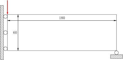
Figure 1: The design domain, boundary conditions and external load for a MBB beam

Table 1: The comparison between the SIMP and CDT.

Method	Structures	Steps	Compliace
SIMP		41	169.2908
CDT		28	164.7108

4.2 Cantilever Beam

The second test example is the classical Cantilever problem (see Figure 2). The beam is fixed along its left side with a downward traction applied at its right middle point. The example consists of $180\times 60$ quad meshes and the target volume fraction is $\mu_{c}=0.6$. Numerical results by both the CDT and SIMP are shown in Figure 3.

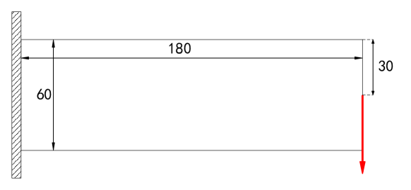
Figure 2: A test example of the benchmark Cantilever problem at volume fraction of 0.5.

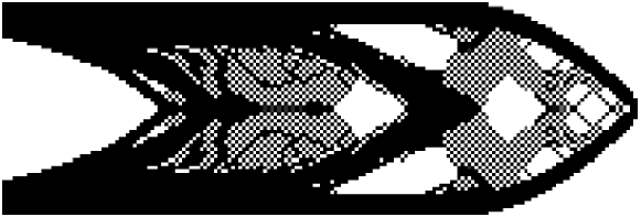
(a) SIMP without filter: compliance = 152.7490 with 37 iterations

(b) CDT: compliance = 153.6767 with 23 iterations

Figure 3: Topology optimization for the cantilever beam by the SIMP (a) and CDT (b) methods.

4.3 Summary of Computational Results

The computational results for the above benchmark problems show clearly that without filter, the SIMP produces a large range of checkerboard patterns and gray elements, while by the CDT method, precise void-solid optimal structure can be obtained with very few checkerboard patterns. By the fact that the optimal density distribution $\rho$ can be obtained analytically at each iteration, the CDT method produces desired optimal structure within much less computing time. The convergence of the CDT method depends mainly on the parameter $\mu\in[\mu_{c},1)$. Generally speaking, the smallar $\mu$ produces fast convergent but less optimal results. Detailed study on this issue will be addressed in the future research.

- (1) Andreassen, E., Clausen, A., Schevenels, M., Lazarov, B.S. and Sigmund, O. Efficient topology optimization in MATLAB using 88 lines of code. Structural and Multidisciplinary Optimization, 43(1):1–16, 2011.
- (2) Ali, E.J. and Gao, D.Y. (2016). Improved Canonical Dual Finite Element Method and Algorithm for Post Buckling Analysis of Nonlinear Gao Beam, Canonical Duality-Triality: Unified Theory and Methodology for Multidisciplinary Study, D.Y. Gao, N. Ruan and V. Latorre (eds). Springer.
- (3) Bendsoe MP. Optimal shape design as a material distribution problem. Structural Optimization, 1:193 C202, 1989.
- (4) Bendsoe MP and Kikuchi N. Generating optimal topologies in structural design using a homogenization method. Computer Methods in Applied Mechanics and Engineering, 72(2):197–224, 1988.
- (5) Gao, D.Y.: Panpenalty finite element programming for limit analysis, Computers & Structures 28, 749–755 (1988)
- (6) Gao, D.Y.: Complementary finite element method for finite deformation nonsmooth mechanics. J. Eng. Math., 30, 339–353 (1996)
- (7) Gao, D.Y.: Canonical duality theory: unified understanding and generalized solutions for global optimization. Comput. & Chem. Eng. 33, 1964–1972 (2009)
- (8) Gao, D.Y. Duality Principles in Nonconvex Systems: Theory, Methods and Applications, Kluwer Academic Publishers, Dordrecht /Boston /London, xviii + 454pp (2000)
- (9) Gao, D.Y.: Solutions and optimality to box constrained nonconvex minimization problems. J. Indust. Manage. Optim. 3(2), 293–304 (2007)
- (10) Gao, D.Y.: On unified modeling, theory, and method for solving multi-scale global optimization problems, AIP Conference Proceedings 1776, 020005 (2016); doi: http://dx.doi.org/10.1063/1.4965311
- (11) Gao, D.Y., Ruan, N.: Solutions to quadratic minimization problems with box and integer constraints. J. Glob. Optim. 47, 463–484 (2010)
- (12) Gao, D.Y., Strang, G.: Geometric nonlinearity: Potential energy, complementary energy, and the gap function. Quart. Appl. Math. 47(3), 487–504 (1989)
- (13) Karp, R.K., Reducibility among combinatorial problems. In R. E. Miller and J. W. Thatcher, editors, Complexity of Computer Computations, page 85-103, New York: Plenum, 1972.
- (14) Moreau, J.J.: La notion de sur-potentiel et les liaisons unilatérales en élastostatique. C.R. Acad. Sci. Paris 267 A, 954–957 (1968)
- (15) Santos, H.A.F.A., Gao D.Y.: Canonical dual finite element method for solving post-buckling problems of a large deformation elastic beam. Int. J. Nonlinear Mechanics 7, 240 – 247 (2011)
- (16) Sigmund, O. A 99 line topology optimization code written in matlab. Structural and Multidisciplinary Optimization, 21(2):120–127, 2001.
- (17) Sigmund, O. and Petersson, J. Numerical instabilities in topology optimization: A survey on procedures dealing with checkerboards, mesh-dependencies and local minima. Structural Optimization, 16(1):68–75, 1998.
- (18) Sigmund, O. and Maute, K. Topology optimization approaches: a comparative review. Structural and Multidisciplinary Optimization, 48(6):1031–1055, 2013.
- (19) Sokolowski J and Zochowski A. On the topological derivative in shape optimization. Structural Optimization, 37:1251–1272, 1999.
- (20) Stolpe, M. and Bendsoe, M.P. Global optima for the Zhou-Rozvany problem. Structural and Multidisciplinary Optimization, 43(2):151–164, 2011.
- (21) van Dijk, N.P., Maute, K., Langelaar, M. and van Keulen, F. Level-set methods for structural topology optimization: a review. Structural and Multidisciplinary Optimization, 48(3):437–472, 2013.