CMB Lens Sample Covariance and Consistency Relations

Abstract

Gravitational lensing information from the two and higher point statistics of the CMB temperature and polarization fields are intrinsically correlated because they are lensed by the same realization of structure between last scattering and observation. Using an analytic model for lens sample covariance, we show that there is one mode, separately measurable in the lensed CMB power spectra and lensing reconstruction, that carries most of this correlation. Once these measurements become lens sample variance dominated, this mode should provide a useful consistency check between the observables that is largely free of sampling and cosmological parameter errors. Violations of consistency could indicate systematic errors in the data and lens reconstruction or new physics at last scattering, any of which could bias cosmological inferences and delensing for gravitational waves. A second mode provides a weaker consistency check for a spatially flat universe. Our analysis isolates the additional information supplied by lensing in a model independent manner but is also useful for understanding and forecasting CMB cosmological parameter errors in the extended $\Lambda$CDM parameter space of dark energy, curvature and massive neutrinos. We introduce and test a simple but accurate forecasting technique for this purpose that neither double counts lensing information nor neglects lensing in the observables.

I Introduction

Power spectra of the cosmic microwave background (CMB) anisotropies have been extremely valuable in helping to confirm predictions of the standard $\Lambda$CDM cosmological model and constrain values of cosmological parameters Ade et al. (2016a). Only recently has gravitational lensing of the CMB been detected, first through cross-correlation with galaxy surveys Smith et al. (2007); Hirata et al. (2008); Hanson et al. (2013), and then by internal correlations of the temperature ($T$) Das et al. (2011); Keisler et al. (2011); Ade et al. (2014), and polarization ($E$,$B$) Keisler et al. (2015); Ade et al. (2016b, c); Sherwin et al. (2016) fields, adding a new source of cosmological information. This secondary signal depends on growth of structure in the universe, which can be leveraged to break certain parameter degeneracies in the CMB data and used to better constrain sum of neutrino masses and other parameters in models beyond $\Lambda$CDM (see Lewis and Challinor (2006) for a review).

Information carried by the lensing potential $\phi$ can be recovered either by measuring its effect on CMB power spectra, in particular the smoothing of the acoustic peaks Seljak (1996) or by measuring four point functions of the temperature and polarization maps. The latter is possible, because gravitational lensing generates a correlation between measured CMB fields and their gradients Zaldarriaga (2000); Hu (2001); Hu and Okamoto (2002), modifying the simple Gaussian statistics of the unlensed CMB. This non-Gaussian structure can be used to measure the lensing potential, for example using a quadratic reconstruction Okamoto and Hu (2003) or iterative delensing Hirata and Seljak (2003); Smith et al. (2012). The reconstructed potential then serves as a new cosmological observable.

The same non-Gaussianity that makes lensing reconstruction possible is responsible for correlating the CMB observables and complicates their analysis. Gravitational lensing induces nontrivial covariances between the lensed temperature and polarization data Benoit-Levy et al. (2012); Schmittfull et al. (2013). Neglecting these covariances can affect parameter forecasts of future experiments and analysis of their data.

In particular, future experiments are expected to have their lensing information limited by sample variance of the lenses: the fact that on the same patch of sky, the gravitational lensing of all CMB observables is due to the same realizations of a finite number of lens modes. In this work we use an extension of the analytical model of Ref. Benoit-Levy et al. (2012) to include covariances between power spectra $C^{XY}_{\ell}$ of the lensed CMB temperature and polarizations with the power spectra of the reconstructed lensing potential, recently also discussed in Green et al. (2016); Peloton et al. (2016). With this model we then investigate how these covariances affect parameter forecasts and construct sharp consistency relations between the two types of observables that can be used to test for foregrounds, systematics or new physics.

The outline of the paper is as follows. In §II we present the analytical model for lens sample covariances. We analyze their impact on cosmological parameters in §III and separate information on them into lensing and non-lensing based sources. Based on this separation, we determine the modes that most strongly covary between CMB power spectra and lens reconstruction in §IV. These provide consistency relations between observables that are largely immune to lens sample variance and cosmological parameter uncertainties. We discuss these results in §V. In the Appendix we use these results to develop a new accurate but simple Fisher forecasting technique in the extended $\Lambda$CDM parameter space that avoids double counting lensing information, and compare it with other similar but less accurate approaches.

II Analytic lens covariance model

In this section, we present an analytical model describing non-Gaussian covariances between the $C_{\ell}^{xy}$ power and cross spectra observables induced by gravitational lensing through the same lenses on the sky. Here these $xy$ spectra are the CMB temperature power spectra $TT$, $E$-mode polarization power $EE$, temperature-polarization cross spectra $TE$, $B$-mode polarization power $BB$ and the power spectrum of the lens potential $\phi\phi$.

As a notational short hand, we denote the subset of $xy$ that includes only the CMB power spectra with capital letters $XY$: $xy\in\{XY,\phi\phi\}$, whereas $XY\in\{TT,EE,TE,BB\}$. Note that although the $T\phi$ and $E\phi$ spectra are also observable we omit them as a source of information but include them in the covariance of other spectra. We comment more on this choice in §III. Covariances predicted by this model have been tested against numerical simulations in Benoit-Levy et al. (2012) for the $XY$ power spectra; here we use the physical intuition gained in Benoit-Levy et al. (2012) to extend the same model to include their covariance with measurements of ${\phi\phi}$. A similar model has recently been also used in Green et al. (2016); Peloton et al. (2016).

Figure 1: Comparison of the lensing potential power spectra $C^{\phi\phi}_{\ell}$ (solid) with the reconstruction noise forecast in this work (dashed, see text for details). The forecast is lens sample variance limited for $\ell\lesssim 10^{3}$.

In this model the correlation matrix is split into “Gaussian part” $\mathcal{G}$ that is diagonal in multipole space and $\mathcal{N}$ which describes non-Gaussian correlations between multipoles,

$$\mathrm{Cov}^{xy,wz}_{\ell\ell^{\prime}}=\mathcal{G}^{xy,wz}_{\ell\ell^{\prime}}+\mathcal{N}^{xy,wz}_{\ell\ell^{\prime}}.$$ (1)

The Gaussian part is modelled after the covariance of Gaussian random fields as

$$\mathcal{G}^{xy,wz}_{\ell\ell^{\prime}}=\frac{\delta_{\ell\ell^{\prime}}}{2\ell+1}\left[C_{\mathrm{exp},\ell}^{xw}C_{\mathrm{exp},\ell}^{yz}+C_{\mathrm{exp},\ell}^{xz}C_{\mathrm{exp},\ell}^{yw}\right],$$ (2)

where the expectation value of the experimentally measured lensed CMB power spectra $C^{xy}_{\mathrm{exp}}$ includes the noise power spectrum $N_{\ell}^{xy}$

$$C_{\mathrm{exp},\ell}^{xy}=C_{\ell}^{xy}+N_{\ell}^{xy}.$$ (3)

For noise in temperature and polarizations, we assume a Gaussian noise spectra Knox (1995)

$$N_{\ell}^{XY}=\Delta_{XY}^{2}e^{\ell(\ell+1){\theta_{\mathrm{FWHM}}^{2}}/{8\log 2}},$$ (4)

where $\Delta_{XY}$ is the instrumental noise (in $\mu$K-radian) and $\theta_{\mathrm{FWHM}}$ is the beam size (in radians).

In this work we investigate a simplified experimental setup of a full sky experiment with specifications inspired by CMB Stage 4 Abazajian et al. (2016). We consider a $1^{\prime}$ beam, $\Delta_{TT}=1\,\mu$K^′, $\Delta_{EE}=\Delta_{BB}=1.4\,\mu$K^′, and $\Delta_{TE}=\Delta_{TB}=\Delta_{EB}=0$ and use measurements from $\ell=2-3000$. CMB Stage 4 measurements at $\ell>3000$ have negligible impact on our results (see §III and IV).

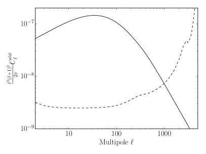
We also assume measurements of $C_{\ell}^{\phi\phi}$ from $\ell=2-5000$ with the reconstruction noise $N_{\ell}^{\phi\phi}$ of the minimal variance quadratic estimator Okamoto and Hu (2003), commonly known as $N^{(0)}$ noise bias, and ignore other noise biases and trispectrum terms Schmittfull et al. (2013) (see §V). Comparison of the $C_{\ell}^{\phi\phi}$ with the reconstruction noise for our experiment $N^{\phi\phi}_{\ell}$ is plotted in Figure 1. Notice that for these specifications, the lens reconstruction is sample variance dominated for $\ell\lesssim 10^{3}$. This is the fundamental assumption underlying this work: that lens sample variance will in the future dominate the measurements of the lens power spectrum at low multipoles. The consistency check proposed in §IV can be viewed as an operational test of this assumption and we comment more on current simulation-based tests in §V.

Figure 2: Correlation matrix $R^{XY,{\phi\phi}}_{\ell_{XY},\ell_{{\phi\phi}}}$ (8) between the $C_{\ell}^{XY}$ CMB power spectra and the power spectra of the reconstructed lensing potential $C_{\ell}^{{\phi\phi}}$. Barely visible features for $\ell_{XY}=\ell_{{\phi\phi}}\lesssim 50$ in the first three panels represent contributions from the Gaussian terms due to nonzero $C_{\ell}^{T\phi},C_{\ell}^{E\phi}$.

Even if we assume that the unlensed CMB fields $\tilde{X}$ and $\phi$ are Gaussian, the lensed CMB fields $X$ are not. In our model, we take two non-Gaussian terms to compose the full covariance,

$$\mathcal{N}^{xy,wz}_{\ell\ell^{\prime}}=\mathcal{N}^{(\phi)xy,wz}_{\ell\ell^{\prime}}+\mathcal{N}^{(E)xy,wz}_{\ell\ell^{\prime}},$$ (5)

which we now describe.

Gravitational lensing induces non-Gaussian covariances between the data because all power spectra are affected by the same realization of the lensing potential; sample variance fluctuations of the lensing power produce coherent changes in all the observed power spectra. The effect accumulates over the whole multipole range of the lenses and is largest for those $C^{XY}_{\ell}$ which are most strongly affected by lensing. It is modeled by adding an extra term

$$\mathcal{N}^{(\phi)xy,wz}_{\ell\ell^{\prime}}=\sum_{L}\frac{\partial{C_{\ell}^{xy}}}{\partial C_{L}^{{\phi\phi}}}\mathrm{Cov}^{{\phi\phi}}_{LL}\frac{\partial{C_{\ell^{\prime}}^{wz}}}{\partial C_{L}^{{\phi\phi}}}$$ (6)

to the non-Gaussian covariance $\mathcal{N}$. The power spectra derivatives are in practice calculated using a two point central difference scheme from results obtained using CAMB Lewis and Bridle (2002). For the reconstructed potential we take $\mathcal{N}^{(\phi){\phi\phi},{\phi\phi}}_{\ell\ell^{\prime}}=0$ as the corresponding variance is part of the Gaussian term.

Sample variance of the unlensed $\tilde{E}\tilde{E}$ power spectrum and its coherent propagation into the lensed power spectra through gravitational lensing produces similar but typically weaker effects. Following Benoit-Levy et al. (2012) we include this contribution only for $\mathrm{Cov}^{XY,BB}_{\ell\ell^{\prime}}$ with

$$\mathcal{N}^{(E)XY,BB}_{\ell,\ell^{\prime}}=\sum_{L}\frac{\partial{C_{\ell}^{XY}}}{\partial C_{L}^{\tilde{X}\tilde{Y}}}\mathrm{Cov}^{\tilde{X}\tilde{Y},\tilde{E}\tilde{E}}_{L,L}\frac{\partial{C_{\ell^{\prime}}^{BB}}}{\partial C_{L}^{\tilde{E}\tilde{E}}}.$$ (7)

Other sample covariance effects from unlensed fields on $XY$ are negligible in comparison Benoit-Levy et al. (2012). We also assume that the analogous terms involving the reconstruction noise, e.g. $\partial N_{l}^{\phi\phi}/\partial C_{L}^{\tilde{E}\tilde{E}}$ and other non-Gaussian reconstruction terms are negligible. This should be a good approximation in the lens sample dominated regime $\ell\lesssim 10^{3}$ (see §V).

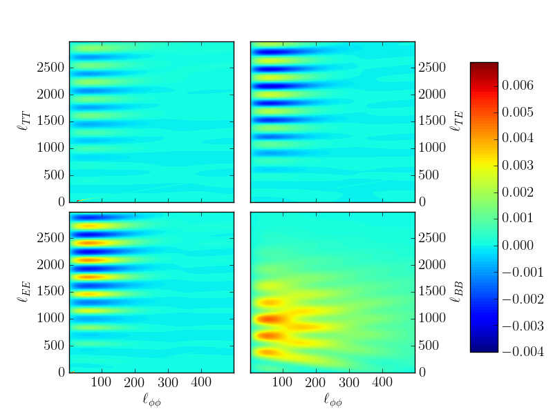
The covariances $\mathrm{Cov}^{XY,WZ}$ we obtain for the CMB power spectra qualitatively agree with those plotted in Fig. 1 of Benoit-Levy et al. (2012) for the same analytical model for covariances but for a slightly different cosmological model. The less well studied covariances $\mathrm{Cov}^{XY,{\phi\phi}}$ are shown in Figure 2; for illustrative purposes we plot the correlation coefficient

$$R^{XY,{\phi\phi}}_{\ell\ell^{\prime}}=\frac{\mathrm{Cov}^{XY,{\phi\phi}}_{\ell\ell^{\prime}}}{\sqrt{\mathrm{Cov}^{XY,XY}_{\ell\ell}\mathrm{Cov}^{{\phi\phi},{\phi\phi}}_{\ell^{\prime}\ell^{\prime}}}}.$$ (8)

In this plot we assume experimental and reconstruction noise for our reference experiment.

We see that the covariances peak for $\ell^{\prime}=\ell_{\phi\phi}\sim 100-200$ which reflects the fact that most of the lensing is caused by lenses at these scales. In covariances with $TT,TE$ and $EE$ there are alternating regions of positive and negative correlations, corresponding to smearing of the peaks and troughs; correlation with $BB$ also shows acoustic features due to oscillations in the unlensed $C^{\tilde{E}\tilde{E}}_{\ell}$ on top of a positive definite contribution. The broad band $BB$ power thus coherently covaries with the lens power Smith et al. (2004). These results also agree with Ref. Green et al. (2016); Peloton et al. (2016).

III Parameter forecasts

In this section we investigate the impact of lens sample covariances between measurements of CMB power spectra and the lensing potential on cosmological parameters. This impact comes through the additional information that lensing supplies on parameters. We show that to good approximation this information in the lensed CMB power spectra can be considered independently from that of the unlensed CMB power spectra, effectively as direct measurements of the lens power spectrum itself.

III.1 Cosmological parameters

In this work we focus on extensions of the standard 6 parameter $\Lambda$CDM cosmological model which we allow to vary two at a time: the sum of masses of the neutrino species $\sum m_{\nu}$, the dark energy equation of state $w$, and the spatial curvature $\Omega_{K}$. For the $\Lambda$CDM parameters we take $\Omega_{b}h^{2}$, the physical baryon density; $\Omega_{c}h^{2}$, the physical cold dark matter density; $n_{s}$, the tilt of the scalar power spectrum; $A_{s}$, its amplitude; and $\tau$, the optical depth to recombination. We choose $\theta$, the angular scale of the sound horizon at recombination, as opposed to the Hubble constant $h$, as the sixth independent parameter given the angular diameter distance degeneracy between $h$ and parameters such as $w$ and $\Omega_{K}$ in the unlensed CMB. This choice also improves the numerical stability of forecasts. We also assume that tensor modes are negligible so that there is no unlensed $B$ mode. We call a set of 8 cosmological parameters of the extended $\Lambda$CDM family $\theta_{A}$. Values of the cosmological parameters for the fiducial model used in this work are summarized in Table 1.

Our assumptions about measurement noise and characterization of lens sample variance in the covariance matrix are summarized in the previous section. In general, we forecast parameter errors given a covariance matrix of a set of observables $D_{i}$ using the Fisher matrix

$$F_{AB}=\sum_{ij}\frac{\partial D_{i}}{\partial\theta_{A}}\,\mathrm{Cov}^{-1}_{ij}\,\frac{\partial D_{j}}{\partial\theta_{B}}.$$ (9)

The inverse Fisher matrix represents an estimate of the covariance matrix of the parameters

$$\mathrm{Cov}_{\theta_{A},\theta_{B}}=(F_{AB})^{-1}.$$ (10)

Prior information is included by adding its Fisher matrix before inverting.

Table 1: Fiducial parameters used in the analysis with extensions to the standard $\Lambda$CDM parameters listed last.

Parameter	Fiducial value
$h$	0.675
$\Omega_{c}h^{2}$	0.1197
$\Omega_{b}h^{2}$	0.0222
$n_{s}$	0.9655
$A_{s}$	$2.196\times 10^{-9}$
$\tau$	0.06
$\sum m_{\nu}$	60 meV
$w$	$-1$
$\Omega_{K}$	0

In Figure 3 we compare how the Fisher forecasts on the two extensions of $\Lambda$CDM change when we neglect the effect of $\mathrm{Cov}^{XY,{\phi\phi}}$, the lens sample covariances between the CMB and lens power spectra. In these plots, $\Lambda$CDM parameters are marginalized over and the third $\Lambda$CDM extension fixed. While for $w$ and $m_{\nu}$, the effect is sizable and amounts to $\sim 20\%$, for $\Omega_{K}$ and $m_{\nu}$ the effect is much smaller. These differences reflect parameter degeneracies in the lensing observables.

Figure 3: Forecasts for 2 parameter extensions to $\Lambda$CDM: $w$-$\sum m_{\nu}$ (left) and $\Omega_{K}$-$\sum m_{\nu}$ (right). Black curves show $\Delta\chi^{2}=1$ constraints considering the full covariance (solid) and with covariances $\mathrm{Cov}^{XY,{\phi\phi}}$ neglected (dashed); $\Lambda$CDM parameters are marginalized over. The blue curves show the same constraints with $\Lambda$CDM parameters fixed to their fiducial values.

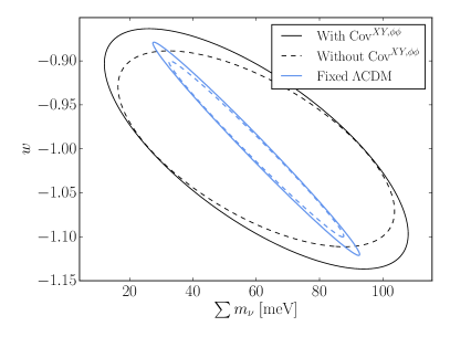
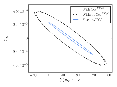
We also show in Figure 3 the same constraints with the 6 $\Lambda$CDM parameters fixed. It is clear that the best constrained direction is limited by parameter degeneracies, especially with $\Omega_{c}h^{2}$ Smith et al. (2006). The worst constrained direction is limited instead by the ability of lensing or other constraints to separate the two additional parameters.

Conversely, in the $\Lambda$CDM model with only the 6 standard parameters varied, parameter errors change by less that 4% when neglecting $\mathrm{Cov}^{XY,{\phi\phi}}$. This reflects the fact that these parameters are well-constrained even in the absence of lensing.

One of the motivations for the rest of the paper will be to understand these behaviors in terms of the additional versus redundant information that lensing observables supply. From the redundant information we will construct sharp consistency tests whose violation would imply systematic errors or violations of fundamental physical assumptions.

Note also that constraints on cosmological parameters depend strongly on how well $\tau$ is constrained whereas those on the lensing power spectrum $C_{\ell}^{\phi\phi}$ itself do not Smith et al. (2006). For the measurements to cleanly separate $C_{\ell}^{\phi\phi}$ information, we primarily need the unlensed CMB in the acoustic regime $C_{\ell}^{\tilde{X}\tilde{Y}}$ to be well-characterized. On the other hand, in terms of cosmological parameters, the amplitude of these spectra in this regime is proportional to $A_{s}e^{-2\tau}$. The leverage on cosmological parameters gained through comparing the initial amplitude $A_{s}$ to the growth-dependent lensing amplitude depends on how well $\tau$ is measured. In our experimental setup we assumed for simplicity that polarization information will be obtained for the full range of multipoles $\ell=2-3000$, which results in a nearly cosmic variance limited constraint on $\tau$ of $\sigma(\tau)\approx 0.002$. This is about five times better than current best constraints from Planck Adam et al. (2016) and furthermore assumes a fixed functional form for reionization Hu and Holder (2003); Heinrich et al. (2016). If the final Planck release does not improve these constraints to substantially below $\sigma(\tau)\sim 0.01$, this uncertainty will dominate the interpretation of lensing constraints for cosmological parameters Smith et al. (2006); Allison et al. (2015) since it will be difficult to improve using ground-based instruments.

More concretely, removing polarization data from $\ell<30$ from our forecasts and replacing it with a prior of $\sigma_{\tau}=0.01$, the errors in the worst constrained direction in Figure 3 do not significantly change, while those in the best constrained direction degrade by roughly a factor of two. On the other hand, characterizing the information on the power spectrum of the lenses does not depend strongly on the measurements of $\tau$ and this will be the main focus of the remainder of this work.

III.2 Lens and unlensed information

CMB information on a given cosmological parameter comes both from its effect on the unlensed CMB power spectra $C_{\ell}^{\tilde{X}\tilde{Y}}$ with $\tilde{X}\tilde{Y}\in\tilde{T}\tilde{T},\tilde{T}\tilde{E},\tilde{E}\tilde{E}$ and on the lenses $C_{\ell}^{\phi\phi}$. It is conceptually useful to separate these sources of information. Indeed, beyond the cosmological parameters considered in the previous section, the total information in the CMB observables is carried by all two point functions for $\tilde{T},\tilde{E},\tilde{B},\phi$, assuming they obey Gaussian statistics; recovery of this complete set of information is the ultimate goal of CMB delensing efforts. By first extracting the lensing information we can also further separate the information from lensed CMB power spectra and reconstruction. The latter can be used to form consistency tests between the two sources of lensing information.

Indeed, the Planck satellite found a mild discrepancy between the amount of lensing present in the $TT$ power spectrum and the $TT$ reconstructed lensing potential Aghanim et al. (2016). While these sources of lensing information are still limited by noise rather than by lens sample variance, if such discrepancies persist in future experiments, they may indicate systematic errors in the experiment or the data analysis technique which could obstruct delensing efforts. By checking for consistency at the power spectra level, one can provide proof against such problems before making incorrect cosmological inferences.

In principle the full implementation of this approach would be to consider every multipole in $C_{\ell}^{\tilde{X}\tilde{Y}}$ and $C_{\ell}^{\phi\phi}$ as a parameter in its own right. However, since the high redshift universe is well described by a $\Lambda$CDM-like model, we choose to parameterize the unlensed power spectra $C_{\ell}^{\tilde{X}\tilde{Y}}$ in terms of a small number of parameters $\tilde{\theta}_{A}$. These $\tilde{\theta}_{A}$ change the unlensed power spectra in exactly the manner of the $\Lambda$CDM parameters $\theta_{A}$, but unlike those, they have no effect on $C_{\ell}^{\phi\phi}$.

The lens power spectrum is instead described by a more complete set of parameters $p_{\alpha}$, reflecting the wider range of possibilities during the acceleration epoch. For practical reasons, instead of considering each multipole $C_{\ell}^{\phi\phi}$ of the lensing potential as a parameter, we assume that the power spectrum is sufficiently smooth in $\ell$ that we can approximate it with binned perturbations around the fiducial model. We then define a set of parameters $p_{\alpha}$ by

$$\ln C^{\phi\phi}_{\ell}\approx\ln C^{\phi\phi}_{\ell}\Big{|}_{\mathrm{fid}}+\sum_{\alpha=1}^{N_{\phi}}p_{\alpha}B_{\alpha}^{\phi,\ell},$$ (11)

where $B_{\alpha}^{\phi,\ell}$ describes the binning and is defined as

$$B^{\phi,\ell}_{\alpha}=\begin{cases}1&\ell_{\alpha}\leq\ell<\ell_{\alpha+1}\\ 0&\mathrm{otherwise}\end{cases}.$$ (12)

Expansion in $\ln C_{\ell}^{{\phi\phi}}$ is chosen to assure positivity of the power spectrum. Any cosmological model which predicts a smooth variation of $\ln C^{\phi\phi}_{\ell}$ from the fiducial model can be captured in these parameters as

$$p_{\alpha}=\frac{1}{\Delta\ell_{\alpha}}\sum_{\ell}B^{\phi,\ell}_{\alpha}\delta\ln C^{\phi\phi}_{\ell},$$ (13)

where $\Delta\ell_{\alpha}=\ell_{\alpha+1}-\ell_{\alpha}$ is the width of bin $\alpha$. We consider uniform binning with bins of width 5 in this paper; we do not expect binning to have any effect on our conclusions. Changes to the lensing potential are allowed up to $\ell=5000$, given by the $\ell$ range in which we assume the reconstruction data are measured.

The full set of parameters which we will constrain with a Fisher analysis is then

$$P_{\mathrm{tot}}=\{\tilde{\theta}_{1},\tilde{\theta}_{2},\dots,p_{1},p_{2},\dots\},$$ (14)

where $\tilde{\theta}_{A}$ only affect the unlensed power spectra and $p_{\alpha}$ only affect the lensing potential. A given cosmological parameter $\theta_{A}$ jointly changes $\tilde{\theta}_{A}$ and $p_{\alpha}$.

In principle to fully represent a cosmological parameter in this way we would have to account for the covariance between the lens power spectrum and the unlensed CMB spectra induced by $C_{\ell}^{\tilde{T}\phi},C_{\ell}^{\tilde{E}\phi}$ – the ISW-lens and reionization-lens correlations respectively. We could in principle add these as parameters to form a complete description. However, these appear only on the largest, severely cosmic variance limited scales which will also be difficult to extract due to foregrounds and systematics. For this reason we completely neglect them from this section onwards by setting $C_{\ell}^{T\phi}=C_{\ell}^{E\phi}=0$ everywhere, which means also in the Gaussian covariance. We checked that omitting these contributions to the covariance matrix has only a small effect on parameter constraints in Figure 3.

III.3 Independent approximation

We can take the lens vs. unlensed information split of the previous section one step further and assume that the data constrain parameters of this split independently so that the $\tilde{\theta}_{A}$ and $p_{\alpha}$ errors do not covary. To the extent that this approximation is true, we can consider the lens information as independent. Physically, this approximation involves the assumption that changes in the unlensed CMB and lens power spectra do not produce degenerate effects in the lensed CMB. We can test this approximation by comparing cosmological parameter constraints on $\theta_{A}$ as constructed from $\tilde{\theta}_{A}$ and $p_{\alpha}$ with the direct forecasts.

Under this approximation we first construct independent Fisher matrices in the $p_{\alpha}$ space

$${F_{\alpha\beta}^{\mathrm{lenses}}=} \sum_{\begin{subarray}{c}\text{$\ell,\ell^{\prime}$}\\ \text{$xy,wz$}\end{subarray}}\frac{\partial C^{xy}_{\ell}}{\partial p_{\alpha}}\left(\mathrm{Cov}^{xy,wz}_{\ell\ell^{\prime}}\right)^{-1}\frac{\partial C^{wz}_{\ell^{\prime}}}{\partial p_{\beta}}$$ (15)

with the unlensed CMB spectra $C_{\ell}^{\tilde{X}\tilde{Y}}$ fixed to their fiducial values and the $\tilde{\theta}_{A}$ space

$$F_{AB}^{\mathrm{unl}} = \sum_{\begin{subarray}{c}\text{$\ell,\ell^{\prime}$}\\ \text{$XY,WZ$}\end{subarray}}\frac{\partial C^{XY}_{\ell}}{\partial\tilde{\theta}_{A}}\left(\mathrm{Cov}^{XY,WZ}_{\ell\ell^{\prime}}\right)^{-1}\frac{\partial C^{WZ}_{\ell^{\prime}}}{\partial\tilde{\theta}_{B}}$$ (16)

with $C_{\ell}^{\phi\phi}$ fixed to their fiducial values. Note that $\phi\phi$ has no dependence on $\tilde{\theta}_{A}$ and so those spectra do not enter into the sum.

We can then obtain the total Fisher matrix of the cosmological parameters by the Jacobian transform

$$F_{AB}=F_{AB}^{\mathrm{unl}}+\sum_{\alpha,\beta}\frac{\partial p_{\alpha}}{\partial\theta_{A}}F_{\alpha\beta}^{\mathrm{lenses}}\frac{\partial p_{\beta}}{\partial\theta_{B}}.$$ (17)

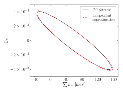
In Figure 4 we compare constraints obtained from the independent model (17) with constraints from the full Fisher analysis. We see that the model indeed works very well and the assumption about independent measurement of the unlensed power spectra and the lensing potential is justified in these examples. As we discuss in §IV.1, spaces that involve $\Omega_{K}$ provide an especially stringent test of the independent approximation.

Because to calculate $F_{AB}^{\mathrm{unl}},F_{\alpha\beta}^{\mathrm{lenses}}$ one needs to know the full covariance matrix for the lensed observables, this split does not represent any practical simplification for calculation of the Fisher matrix unlike the related “additive” approximation in Ref. Smith et al. (2006) that utilizes the unlensed spectra as observables. Conversely, we do not incur errors from conflating unlensed power spectra with direct observables. In Appendix A we introduce a new forecasting approximation which combines the virtues of these two approaches: simplicity and accuracy.

Figure 4: Accuracy of the independent lensing information model of (17) (red dashed) compared with the full Fisher forecast for the cases from Fig. 3 (black solid).

IV Redundancy and Consistency

Given the technique for isolating information about the lens power spectrum introduced in the previous section, we can now assess the level of redundancy and consistency between the information coming from lensed CMB power spectra and lensing power spectrum. This study both helps explain constraints on cosmological parameters and enables the construction of sharp consistency tests between these two aspects of lensing in the data that are nearly immune to sample variance.

IV.1 Consistency of covarying modes

We can use the Karhunen-Loève (KL) transform to extract the modes or linear combinations of the lens parameters $p_{\alpha}$ that are most impacted by the $\mathrm{Cov}^{XY,{\phi\phi}}$ covariance between the measurements of the lensed CMB power spectra $C_{\ell}^{XY}$ and the lens power spectra $C_{\ell}^{\phi\phi}$. These modes carry redundant information between $XY$ and $\phi\phi$ that can be used as a consistency check on the data and analysis techniques.

To assess the impact of the $XY,{\phi\phi}$ covariance, we consider two versions of the inverse Fisher matrix for $p_{\alpha}$,

$$\mathrm{Cov}_{\alpha\beta}=[F_{\alpha\beta}^{\rm lenses}]^{-1},$$ (18)

from Eq. (15), and

$$\mathrm{Cov}_{\alpha\beta}^{-}=[F_{\alpha\beta}^{\rm lenses}]^{-1}\Big{|}_{\mathrm{Cov}^{XY,{\phi\phi}}_{\ell\ell^{\prime}}=0},$$ (19)

the same construction but with the $XY,\phi\phi$ covariance artificially set to zero.

We can then perform a KL transformation by finding all solutions to the generalized eigenvalue problem

$$\sum_{\beta}\mathrm{Cov}_{\alpha\beta}v^{(k)}_{\beta}=\sum_{\beta}\lambda^{(k)}\mathrm{Cov}_{\alpha\beta}^{-}v^{(k)}_{\beta}.$$ (20)

Here $v^{(k)}_{\beta}$ and $\lambda^{(k)}$ are the KL eigenvectors and eigenvalues. The KL transform of the measurements

$$\Psi^{(k)}=\sum_{\alpha}v^{(k)}_{\alpha}p_{\alpha}$$ (21)

provides a representation that is uncorrelated, or statistically orthogonal, with respect to both covariance matrices since solutions to (20) are simultaneously orthogonal with respect to the metrics defined by the covariance matrices,

$$\mathrm{Cov}_{\Psi^{(k)}\Psi^{(l)}}=\sum_{\alpha\beta}v^{(l)}_{\alpha}\mathrm{Cov}_{\alpha\beta}v^{(k)}_{\beta} = \lambda^{(k)}\delta_{kl},$$

$$\mathrm{Cov}_{\Psi^{(k)}\Psi^{(l)}}^{-}=\sum_{\alpha\beta}v^{(l)}_{\alpha}\mathrm{Cov}_{\alpha\beta}^{-}v^{(k)}_{\beta} = \delta_{kl}.$$ (22)

We order $\lambda^{(k)}$ to be decreasing with $k$ and hence in the ratio of the variances between the two, i.e. the degradation in the constraints due to $\mathrm{Cov}^{XY,{\phi\phi}}_{\ell\ell^{\prime}}$.

The eigenvectors are not necessarily mutually orthonormal in the ordinary Euclidean sense,

$$\sum_{\alpha}v^{(l)}_{\alpha}v^{(k)}_{\alpha}\neq\delta_{kl},$$ (23)

as they would be in an ordinary eigenvector or principal component representation (see §IV.2). Consequently, the forward and inverse KL transforms are distinct:

$$p_{\alpha}=\sum_{k}w^{(k)}_{\alpha}\Psi^{(k)},$$ (24)

where $w^{(k)}_{\alpha}$ is the matrix inverse of $v^{(k)}_{\alpha}$ rather than its transpose. As a function of the $\alpha$ index, $v^{(k)}_{\alpha}$ represents how strongly individual $p_{\alpha}$ contribute to the $k$th KL mode whereas $w^{(k)}_{\alpha}$ represents how the $k$th KL mode is distributed onto the original modes. They can have very different shapes in $\alpha$. We always use the forward KL transform and $v^{(k)}_{\alpha}$ in the following discussion to avoid confusion.

We find two strongly degraded modes with

$$\lambda^{(1)} = 1.86,$$ (25)

$$\lambda^{(2)} = 1.39.$$

These modes would be better constrained if there were no $XY,{\phi\phi}$ covariances, which agrees with the intuitive expectation that neglecting mutual covariances would lead to double counting of the lensing information. The corresponding eigenvectors $v^{(1,2)}_{\alpha}$ are plotted in Figure 5. All other modes are only mildly affected and have eigenvalues between 0.93 and 1.08.

Figure 5: KL components of the lensing potential most affected by the covariances $\mathrm{Cov}^{XY,{\phi\phi}}$ of CMB fields with the reconstructed lensing potential. By neglecting these covariances, constraints on the corresponding amplitude $\Psi^{(k)}$ would be overly optimistic due to double counting of lensing information.

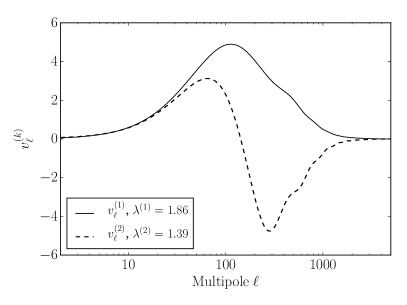
We see that measurements of the amplitude of the first mode $\Psi^{(1)}$ are degraded by almost a factor of two. This means that constraint on this mode obtained from the $XY$ lensed power spectra alone is comparable to a constraint from the reconstructed lensing potential alone but that these two different measurements are highly correlated. This occurs because both these measurements have their variances dominated by the sample variance of the lenses. This sample variance is common to both measurements, which explains why the two variances are comparable and strongly correlated.

Table 2 summarizes how well we can constrain $\Psi^{(1)}$ under various assumptions and provides quantitative justification of these claims. The first two lines summarize the KL results – neglecting $\mathrm{Cov}^{XY,{\phi\phi}}$ leads to a double counting of the lensing information and overly tight constraints in the full dataset. Instead, we can constrain this mode separately from ${\phi\phi}$ and $XY$ data with variances that are both comparable to those of the full dataset. The $XY$ result is not a trivial consequence of the KL results since the KL modes are not specifically constructed to be statistically orthogonal with $XY$ measurements alone. Because the $XY$ power spectra provide only integrated constraints on $C_{\ell}^{\phi\phi}$, we impose a mild theoretical prior of $\sigma_{p_{\alpha}}=1$ to forbid numerical problems and degeneracies induced by unphysically large features in $C_{\ell}^{\phi\phi}$ (see also §IV.2). The minimum variance unbiased linear estimators of $\Psi^{(1)}$ from the separate $\phi\phi$ and $XY$ datasets have a correlation coefficient of 0.77, in agreement with values in Table 2.

Note that even when considering $XY$ separately, we include all of the internal covariances induced by lens sample variance. Without the non-Gaussian covariances $\mathcal{N}$, $\sigma_{\Psi^{(1)}}^{2}$ decreases significantly and is unphysically smaller than the lens sample variance limit by more than a factor of 3. Finally we show that removing all of the non-Gaussian covariances in the full dataset leads to an even more extreme violation of the lens sample variance limit.

Table 2: Variance of KL consistency mode $\Psi^{(1)}$ obtained from various combinations of lensed CMB spectra $XY$ and lens power spectra $\phi\phi$ measurements and assumptions about their variances and covariance.

Dataset	Covariance	$\sigma^{2}_{\Psi^{(1)}}$
$XY,\phi\phi$	$\mathrm{Cov}^{XY,{\phi\phi}}_{\ell\ell^{\prime}}=0$	1.00
$XY,\phi\phi$	Full	1.86
$\phi\phi$	Full	1.96
$XY$	Full	2.26
$\phi\phi$	Sample variance	1.74
$XY$*5	Gaussian	0.52
$XY,\phi\phi$	Gaussian	0.29

Because $\Psi^{(1)}$ is constrained by two independent but strongly correlated measurements, these measurements in principle provide an excellent systematic check on the experimental data that is nearly immune to sample variance and cosmological parameter uncertainties. This check could be very valuable in future experiments, which are likely to be foreground and systematics limited: comparing $\Psi^{(1)}$ measured from power spectra and reconstruction separately could serve as a simple check on data quality and reconstruction algorithms before performing the delensing operation. Identical conclusions are to a lesser degree valid also for $\Psi^{(2)}$, which could also serve as a weaker consistency check, but valuable in its own right for reasons we discuss below.

Next we test the robustness of these results to our assumptions. The eigenvectors $v^{(k)}$ and corresponding eigenvalues do not change appreciably if we discard in temperature and polarization information for $\ell<30$, discard reconstruction information for $\ell>3000$, or include polarization information out to $\ell<5000$. Unlike cosmological parameter inferences that involve breaking parameter degeneracies involving the standard $\Lambda$CDM parameters, $A_{s},\tau,\Omega_{c}h^{2}$, this consistency test involves just the lensing information. In principle, the development of more sophisticated lens reconstruction algorithms beyond the damping tail may in the future allow additional consistency tests with $XY$ power spectra at $\ell>3000$. However, this information does not significantly impact the $\Psi^{(1)}$ consistency test since it involves lens power on comparably high $\ell$ scales. The impact of neglecting $C_{\ell}^{T\phi},C_{\ell}^{E\phi}$ should also not be significant, because unlike $v^{(1,2)}$ they are only significant at the lowest multipoles.

The most important assumption in this construction is that we can independently consider the information about the unlensed CMB and the lens power spectra. While this is a good assumption in the extended $\Lambda$CDM parameter space for the full data set as demonstrated in Fig. 4, it is less true when considering the lensed CMB $XY$ spectra alone if spatial curvature is allowed to vary. Increasing $\Omega_{K}$ impacts the unlensed CMB through $\tilde{\Omega}_{K}$ in a manner similar to the smoothing of the acoustic peaks by lensing Smith et al. (2006). Moreover, its impact on lensing through $p_{\alpha}(\Omega_{K})$ is to decrease the amplitude of power (see Fig. 8 below), and so the overall sensitivity to curvature is degraded from what is assumed in the independent approximation. Furthermore, the total impact of curvature on the lensed power spectrum becomes nearly degenerate with effects of the neutrino mass Smith et al. (2006). On the other hand, $BB$ partially breaks the degeneracy as it is not generated by curvature.

To investigate how severe these degeneracies are in the $XY$ dataset, we compare forecasted errors on $\Psi^{(1,2)}$ with fixed vs.  marginalized $\tilde{\theta}_{A}$ in Table *4. As before, we assume a mild theoretical prior $\sigma_{p_{\alpha}}=1$.

When $\tilde{\Omega}_{K}$ is held fixed, the variances of both $\Psi^{(1)}$ and $\Psi^{(2)}$ are negligibly increased by marginalizing the remaining 8 extended $\Lambda$CDM parameters. When $\tilde{\Omega}_{K}$ is also marginalized the variance of $\Psi^{(1)}$ changes only by $\sim 10\%$ but that of $\Psi^{(2)}$ is close to doubled. This mirrors the fact that changing $\Psi^{(1)}$ changes $BB$ significantly more – relative to the rest of the observables – than $\Psi^{(2)}$ does and cannot be mimicked by curvature in the unlensed spectra. We conclude that $\Psi^{(1)}$ provides a robust consistency test for lensing in the full $\Lambda$CDM+$w$+$\Omega_{K}$+$\sum m_{\nu}$ context whereas inconsistencies in $\Psi^{(2)}$ between $XY$ and $\phi\phi$ measurements may indicate a finite spatial curvature. Violations of consistency in $\Psi^{(1)}$ would indicate systematics and foregrounds in the measurement or new physics at recombination that mimics the effect of lensing. Either of these possibilities would lead to incorrect cosmological inferences and complicate delensing of the CMB if not discovered beforehand.

This relationship between lensing and curvature effects in the unlensed spectrum also leads to the small difference between the full Fisher forecast and the independent lensing information model in Figure 4 which we discuss further in Appendix A.

Table 3: Variance of KL consistency modes $\Psi^{(1,2)}$ obtained from $XY$ lensed CMB power spectra alone with and without unlensed CMB parameters $\tilde{\theta}_{A}$ marginalized.

	$\sigma^{2}_{\Psi^{(1)}}$	$\sigma^{2}_{\Psi^{(2)}}$
all $\tilde{\theta}_{A}$ fixed	2.26	4.13
8 marginalized, $\tilde{\Omega}_{K}$ fixed	2.27	4.35
all $\tilde{\theta}_{A}$ marginalized	2.52	7.34

IV.2 Principal component implementation

The consistency check discussed in §IV.1 involves measuring the KL consistency parameter $\Psi^{(1)}$ from the CMB $XY$ power spectra alone. There are practical obstacles to implementing this measurement given the many ill-constrained modes that compose the full lensing power spectrum $C_{\ell}^{\phi\phi}$ through $p_{\alpha}$. Furthermore, with just $XY$ measurements alone, curvature $\Omega_{K}$ mildly violates the assumption that the unlensed CMB parameters can be independently extracted from the lensed CMB as discussed in the previous section. A full assessment will require going beyond the Fisher approximation with validation on numerical simulations which we postpone to a future work. In this section, we take the first steps toward this goal by re-examining the lensing principal component decomposition introduced in Ref. Smith et al. (2006). A small set of these parameters completely characterizes the lensing information in the $XY$ data and can be measured jointly with those controlling the unlensed parameters $\tilde{\theta}_{A}$, with or without curvature.

The forecasted covariance matrix of the $p_{\alpha}$ lensing parameters measured by $XY$ power spectra is given by the inverse Fisher matrix (15), omitting ${\phi\phi}$ in the sum. The orthonormal eigenvectors $K^{(i)}_{\alpha}$ of this matrix represent an alternate basis for the measurements

$$\Theta^{(i)}=\sum K^{(i)}_{\alpha}p_{\alpha},$$ (26)

that yield uncorrelated parameters, rank ordered by their variance, in principle. By keeping only the eigenvectors that are predicted to have low variance, we can measure the relevant information with a much smaller set of principal components (PCs). Note that this differs from the KL basis in that it rank orders modes by total variance from $XY$ rather than by whether the joint measurements are noise or lens sample variance dominated.

The efficiency of the PC approach depends on the number of components needed to completely characterize the relevant information. In our case, we find eigenvalues

$$10^{3}\lambda = 1.0,4.0,12,19,93,\dots,$$ (27)

which indeed shows that relative importance of the components decreases rapidly and hits the $\sigma_{p_{\alpha}}=1$ prior shortly thereafter.

The five most important components are shown in Figure 6. The low order modes peak where the lenses have their largest impact on $XY$ and the higher modes are increasingly oscillatory, because they have to be orthogonal to the more important eigenmodes.

Figure 6: Five principal components $K^{(i)}_{\ell}$ of the lensing potential best measured by the lensed power spectra.

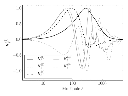
It is sufficient to keep only several principal components to characterize the impact of cosmological parameters or the KL consistency modes completely. Specifically, the mode $\Psi^{(1)}$ can be faithfully constructed from $XY$ measurements of the 5 lowest order PC components with the dominant contributions from the first two. We have explicitly checked that truncating the remaining components has no significant effect on the error analysis, for example as displayed in Table *4. Because of the truncation, the $\sigma_{p_{\alpha}}=1$ prior plays little role and may be omitted. This construction therefore provides a practical means of measuring $\Psi^{(1)}$ in the presence of the many unconstrained but unphysical modes.

We can also measure these $\Theta^{(i)}$ modes with lensing reconstruction and check consistency between $XY$ and $\phi\phi$ directly in PC space. The results are summarized in Table 4. Although the first mode is equally well constrained by $XY$ and $\phi\phi$ measurements, it does not produce as sharp a consistency test as $\Psi^{(1)}$. The reason is that lens sample variance only contributes less than $\sim 2/3$ of the variance of either measurement and their results can therefore differ due to the remaining noise variance. Higher modes are even less sample variance limited in $XY$. This mainly reflects the higher $\ell$ weight in the PC components compared with $\Psi^{(1)}$. We can interpret $\Psi^{(1)}$ as essentially the linear combination of $\Theta^{(1)}$ and $\Theta^{(2)}$ that best isolates the low $\ell$, lens sample variance limited information.

Finally, while in this work we mainly focused on lensing information which is redundant, these results imply that the lensed $XY$ CMB power spectra actually improve constraints on lensing potential above roughly $\ell\sim 500$ (see Tab. 4). In cosmological parameter errors this improvement is hidden because of the degeneracies with $\Lambda$CDM parameters as we discuss next.

Table 4: Variance of $\Theta^{(i)}$ obtained from various datasets under various assumptions about covariances of the data and noise.

Dataset	Covariance	$10^{3}\sigma_{\Theta^{(1)}}^{2}$	$10^{3}\sigma_{\Theta^{(2)}}^{2}$	$10^{3}\sigma_{\Theta^{(3)}}^{2}$	$10^{3}\sigma_{\Theta^{(4)}}^{2}$	$10^{3}\sigma_{\Theta^{(5)}}^{2}$
$XY$	Full	1.0	4.0	12	18	85
$\phi\phi$	Full	1.0	2.4	5.7	8.2	30
$\phi\phi$	Sample variance	0.66	2.0	1.2	0.8	0.4

IV.3 Parameter constraints revisited

The KL analysis exposes the fact that there is one mode which is nearly equally well measured by CMB power spectra $XY$ and lensing reconstruction $\phi\phi$ that reflects a large portion of the nearly lens sample dominated information on $C_{\ell}^{\phi\phi}$ at low $\ell$. Our PC analysis highlights the fact that the decrease in lens sample variance at higher $\ell$ means that despite being the highest in signal to noise, this consistency mode carries only a portion of the total information from lensing on the overall amplitude of the lensing spectrum. Furthermore, as shown in Fig. 3, the constraints from the overall amplitude of the lensing power spectrum on the $\Lambda$CDM extensions is limited by degeneracies since the $\Lambda$CDM parameters $A_{s}$ (implicitly $\tau$) and $\Omega_{c}h^{2}$ also affect $p_{\alpha}$, further reducing the impact of lens sample covariance. It is when the low $\ell$ lensing information strongly breaks a parameter degeneracy that the impact of the $\mathrm{Cov}^{XY,{\phi\phi}}$ covariance is seen.

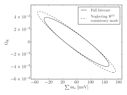
In Figure 7 we show how the parameter constraints would change if we neglect the information carried by the $\Psi^{(1)}$ consistency mode. In both the $w-\sum m_{\nu}$ and $\Omega_{K}-\sum m_{\nu}$ cases, the impact is mainly in the degenerate direction but is only dramatic in the former. The impact of $\mathrm{Cov}^{XY,{\phi\phi}}$ shown in Fig. 3 can be understood from this result since the information on $\Psi^{(1)}$ is essentially double counted if this covariance is neglected.

Figure 7: Impact of eliminating the lens information associated with the KL consistency mode $\Psi^{(1)}$ (dashed line). Solid lines represent the full Fisher forecast from Fig. 3. The consistency mode carries a substantial amount of the total information especially in cases where low $\ell$ lens information breaks parameter degeneracies.

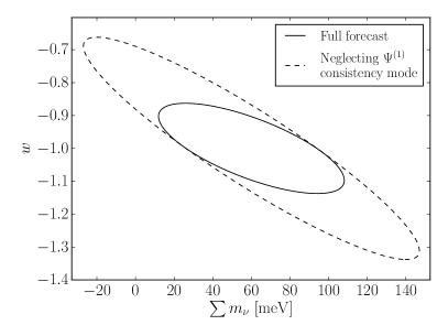
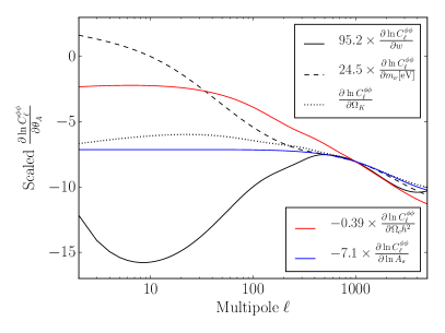
We can further understand the different parameter behaviors by examining the impact of parameters on $p_{\alpha}$ or $\ln C_{\ell}^{\phi\phi}$ (see Fig. 8). Although the measurements determine the amplitude of the $C_{\ell}^{\phi\phi}$ well at $\ell\gtrsim 500$, they are unable to separate out the contributions from the various cosmological parameters. In particular, linear combinations of $\ln A_{s}$ and $\Omega_{c}h^{2}$ can mimic the impact of the extended $\Lambda$CDM parameters Smith et al. (2006). Therefore, while the best constrained direction in the 2-dimensional extended spaces correspond to combinations of the parameters that coherently change $C_{\ell}^{\phi\phi}$ at $\ell\gtrsim 500$, the constraint itself is limited by how well $\ln A_{s}$ and $\Omega_{c}h^{2}$ are measured not by how well $C_{\ell}^{\phi\phi}$ is measured (see Fig. 3). The degenerate or worst constrained direction corresponds to when the parameter variations cancel in their effect.

At $\ell\lesssim 500$ the degeneracy between $w$ and $\Omega_{K}$ or $\sum m_{\nu}$ observed at high $\ell$ starts to break, which allows us to meaningfully constrain also the perpendicular direction in the parameter space. For $\Omega_{K}$ and $\sum m_{\nu}$ this degeneracy breaking is noticeably weaker, especially at $\ell\gtrsim 50$. Given the large sample variance associated with the lowest multipoles, the limiting source of information in the degenerate direction in the $\Omega_{K}-\sum m_{\nu}$ plane comes from the unlensed CMB rather than the lensing information. Hence, the effect of lens sample covariance is smaller in this case.

Finally for these issues that relate to parameter degeneracies, it is important to remember that external information from measurements beyond the CMB, for example from baryon acoustic oscillations, can break these degeneracies and allow more of the information on $C_{\ell}^{\phi\phi}$ that our analysis uncovers to be used for parameter constraints.

Figure 8: Derivatives of $\ln C_{\ell}^{\phi\phi}$ with respect to cosmological parameters $w,\sum m_{\nu},\Omega_{K},\Omega_{c}h^{2},\ln A_{s}$ normalized at $\ell=1000$ to highlight degeneracies. These derivatives are taken at fixed acoustic scale $\theta$.

V Discussion

The lensing observables from the two and higher point statistics of the temperature and polarization fields are intrinsically correlated because they are lensed by the same realization of structure between last scattering and the observer. While currently these observables are noise variance limited, in the future they are expected to be lens sample variance limited. When jointly analyzing these observables, it will then be important to take these correlations into account both to prevent double counting of information and because they provide important consistency checks that are immune to sample variance, the chance fluctuations in the lenses.

In this work, we study a simple analytical model that consistently incorporates the lens sample covariance between CMB power spectra and lens reconstruction from higher point information. This covariance model can be employed for cosmological parameter estimation to build the lens sample variance piece of the likelihood function as well as Fisher forecasts for future experiments.

While there is only a small effect on parameter errors of the covariances between the reconstructed lensing potential and the lensed power spectra in the $\Lambda$CDM and even the extended $\Lambda$CDM context, parameter errors, degeneracies and non-lensing information mask the full impact of the covariance.

To better expose this impact, we work in an approximation where information in the unlensed CMB power spectrum and the lensing potential $C_{\ell}^{\phi\phi}$ are considered independently. Using a Karhunen-Loève analysis, we identify one mode in $C_{\ell}^{\phi\phi}$ that in the future should be nearly lens sample variance limited using either lensed power spectra or lensing reconstruction and hence nearly perfectly covaries between the two. If this covariance is not taken into account then information on this mode will be double counted. This mode peaks at somewhat lower multipole than the bulk of the information on the lensing power spectrum due to the larger signal versus noise variance there.

This mode can be measured separately through lens reconstruction and lensed CMB power spectra with the help of a principal component decomposition of the latter. Notably, inconsistency between the measurements cannot be explained by chance lens realizations or parameter variations, and is immune to ambiguities due to $\tau$, the optical depth to reionization. Instead, violations could indicate systematics, lens reconstruction errors, foregrounds or new physics at recombination which changes the unlensed power spectra, including the $BB$ power spectrum, in ways degenerate with lensing. They would then lead to incorrect cosmological inferences and delensing if not taken into account.

The identification of this mode also explains the impact of covariances between the reconstructed lensing potential and the lensed power spectra on parameter constraints. There is only a small effect within the $\Lambda$CDM model as these parameters are well constrained even without lensing. The impact of covariance is mainly seen when measurements of the low $\ell$ lensing power spectrum are useful in breaking parameter degeneracies in interpreting the measurements at higher $\ell$. Specifically, for $w$ and $\sum m_{\nu}$, the consistency mode has a strong impact on parameters and hence its double counting would lead to constraints overly optimistic by $\sim$ 20%.

There is a second combination of $C_{\ell}^{\phi\phi}$ with similar properties, however there the correlation is weaker. Despite being weaker, statistically significant violations of consistency in this mode are interesting since they may indicate nonzero spatial curvature as it has similar effects on the unlensed CMB as lensing.

While this work was in preparation, a similar analytic approach to modelling covariances was compared against numerical simulations Peloton et al. (2016). That model was found to work well after realization-dependent noise subtraction. As can be seen from their Figs. 3 and 4, these subtractions affect mostly correlations with lensing power spectra above $\ell\sim 1000$ and would be hidden by reconstruction noise in our approach. They also show that the other trispectrum terms to the covariance, which we neglect, are subdominant. Potentially more troublesome is their finding that there are some differences between the analytical model and simulations, especially in $\mathrm{Cov}^{BB,{\phi\phi}}$ at low $\ell_{BB}$ which they claim appears to be statistically significant Peloton . If confirmed, then our analysis implicitly assumes that such additional effects can be modeled without breaking our consistency relations – in essence that both lensed CMB and reconstruction can measure this consistency mode to nearly the lens sample variance limit. More generally, this consistency mode can be used to search for unaccounted for systematics in lens reconstruction. We intend to study these issues and quantify their impact in a future work.

Appendix A Simple forecast methods

In this appendix we compare various Fisher matrix approaches of how to estimate parameter constraints, including the standard calculation which uses the full analytical covariance matrix (1). We also introduce a new forecasting approach, which we call the Simple Lensing Approximation (SLA), that is very accurate in predicting parameter constraints from CMB data only and does not require calculation of the full covariance matrix.

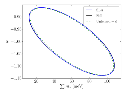
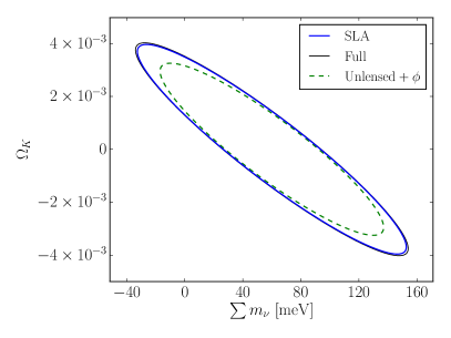
A frequently used approach to avoid double counting of the lensing information is to derive parameter constraints from the unlensed $\tilde{X}\tilde{Y}$ CMB power spectra and the reconstruction of the lensing potential assuming Gaussian statistics in each. These constraints are equivalent to assuming that complete delensing in the CMB maps is possible, that it does not alter their noise properties and that no extra information on the lensing beyond reconstruction can be recovered from the $XY$ power spectra. In the main text we have seen that while the lensing information in $XY$ is substantial, it is largely redundant with reconstruction or limited by parameter degeneracies. For this reason, this approximation works fairly well in the $w-\sum m_{\nu}$ plane. However, as seen from Figure 9, this approximation noticeably underestimates the errors on curvature since its effect on the unlensed spectrum and lensing work in opposite directions in the smoothing of the peaks, degrading the overall curvature sensitivity in the lensed CMB power spectra.

This problem is largely fixed by our independent lensing information model of Eq. (17) which is shown in Fig. 4. In this model, the information from the unlensed power spectra is still considered as separate from that of the lens spectrum but the observable is the lensed $XY$ spectrum and lens sample covariance is taken into account in the covariances of observables. The drawback is that to make forecasts, the cumbersome lens sample covariance matrix must be carried through all pieces of the construction.

We can combine the virtues of these two approaches in a new simple forecasting method, dubbed SLA, if all that is desired are parameter forecasts in the extended $\Lambda$CDM space from the CMB alone. Namely, we can avoid double counting of the lens information by dropping the lens information in the $XY$ power spectra and along with it the non-Gaussian covariances induced by lensing. Importantly, we still use the lensed $XY$ power spectra and not the unlensed $\tilde{X}\tilde{Y}$ power spectra as the observables. Specifically,

$$F^{\mathrm{SLA}}_{AB}=F_{AB}^{\mathrm{unl,SLA}}+\sum_{\alpha,\beta}\frac{\partial p_{\alpha}}{\partial\theta_{A}}F_{\alpha\beta}^{\mathrm{lenses,SLA}}\frac{\partial p_{\beta}}{\partial\theta_{B}}$$ (28)

where we continue to assume Gaussian lens reconstruction noise as in the main text,

$${F_{\alpha\beta}^{\mathrm{lenses,SLA}}=} \sum_{\ell}\frac{\partial C^{{\phi\phi}}_{\ell}}{\partial p_{\alpha}}\left(\mathcal{G}^{{\phi\phi},{\phi\phi}}_{\ell\ell}\right)^{-1}\frac{\partial C^{{\phi\phi}}_{\ell}}{\partial p_{\beta}}.$$ (29)

and omit any lensing information in the $XY$ power spectra. The conceptual difference from Eq. (17) is that when evaluating the unlensed Fisher matrix we assume Gaussian statistics,

$$F_{AB}^{\mathrm{unl,SLA}} = \sum_{\begin{subarray}{c}\text{$\ell$}\\ \text{$XY,WZ$}\end{subarray}}\frac{\partial C^{XY}_{\ell}}{\partial\tilde{\theta}_{A}}\left(\mathcal{G}^{XY,WZ}_{\ell\ell}\right)^{-1}\frac{\partial C^{WZ}_{\ell}}{\partial\tilde{\theta}_{B}}.$$

As before, derivatives in (29) should be evaluated at fixed unlensed power spectra while derivatives in (A) should be evaluated at fixed lensing potential.

We show in Fig. 9 that this approximation provides simple but highly accurate constraints even when curvature is involved. In fact it performs slightly better than the independent approximation of the main text in that it allows lensing to recover information that would otherwise be lost to the non-Gaussian correlations between multipole moments in the $XY$ power spectra. On the other hand, this simple forecast scheme ignores the fact that the $XY$ power spectra provide strong constraints on the lensing power spectra at low multipole that serve as consistency checks against reconstruction measurements and provide additional constraints at high lens multipole when parameter degeneracies are broken by external measurements. This is especially true beyond the $\ell<3000$ limit for polarization measurements tested here but there the astrophysical uncertainties in modeling lenses in the nonlinear regime also limit cosmological parameter information.

Figure 9: New SLA forecasting approximation (solid blue) compared with the full forecast (black solid) and the frequently used approach of using the unlensed spectra and $\phi$ lensing power spectrum (green dashed). The unlensed approach is simple but errs in assuming the unlensed spectra are directly observable. The SLA approach employs the lensed CMB spectra but omits both their lensing information and covariances making it both accurate and simple.

References

- Ade et al. (2016a) P. A. R. Ade et al. (Planck), Astron. Astrophys. 594, A13 (2016a), arXiv:1502.01589 [astro-ph.CO] .
- Smith et al. (2007) K. M. Smith, O. Zahn, and O. Dore, Phys. Rev. D76, 043510 (2007), arXiv:0705.3980 [astro-ph] .
- Hirata et al. (2008) C. M. Hirata, S. Ho, N. Padmanabhan, U. Seljak, and N. A. Bahcall, Phys. Rev. D 78, 043520 (2008).
- Hanson et al. (2013) D. Hanson et al. (SPTpol), Phys. Rev. Lett. 111, 141301 (2013), arXiv:1307.5830 [astro-ph.CO] .
- Das et al. (2011) S. Das et al., Phys. Rev. Lett. 107, 021301 (2011), arXiv:1103.2124 [astro-ph.CO] .
- Keisler et al. (2011) R. Keisler et al., Astrophys. J. 743, 28 (2011), arXiv:1105.3182 [astro-ph.CO] .
- Ade et al. (2014) P. A. R. Ade et al. (The Planck Collaboration), Astron. & Astrophys. 571, A17 (2014), arXiv:1303.5077 .
- Keisler et al. (2015) R. Keisler et al. (SPT), Astrophys. J. 807, 151 (2015), arXiv:1503.02315 [astro-ph.CO] .
- Ade et al. (2016b) P. A. R. Ade et al. (Planck), Astron. Astrophys. 594, A15 (2016b), arXiv:1502.01591 [astro-ph.CO] .
- Ade et al. (2016c) P. A. R. Ade et al. (BICEP2, Keck Array), (2016c), arXiv:1606.01968 [astro-ph.CO] .
- Sherwin et al. (2016) B. D. Sherwin et al., ArXiv e-prints (2016), arXiv:1611.09753 .
- Lewis and Challinor (2006) A. Lewis and A. Challinor, Phys. Rept. 429, 1 (2006), arXiv:astro-ph/0601594 [astro-ph] .
- Seljak (1996) U. Seljak, Astrophys. J. 463, 1 (1996), arXiv:astro-ph/9505109 [astro-ph] .
- Zaldarriaga (2000) M. Zaldarriaga, Phys. Rev. D62, 063510 (2000), arXiv:astro-ph/9910498 [astro-ph] .
- Hu (2001) W. Hu, Phys. Rev. D64, 083005 (2001), arXiv:astro-ph/0105117 [astro-ph] .
- Hu and Okamoto (2002) W. Hu and T. Okamoto, Astrophys. J. 574, 566 (2002), arXiv:astro-ph/0111606 [astro-ph] .
- Okamoto and Hu (2003) T. Okamoto and W. Hu, Phys. Rev. D67, 083002 (2003), arXiv:astro-ph/0301031 [astro-ph] .
- Hirata and Seljak (2003) C. M. Hirata and U. Seljak, Phys. Rev. D68, 083002 (2003), arXiv:astro-ph/0306354 [astro-ph] .
- Smith et al. (2012) K. M. Smith, D. Hanson, M. LoVerde, C. M. Hirata, and O. Zahn, JCAP 1206, 014 (2012), arXiv:1010.0048 [astro-ph.CO] .
- Benoit-Levy et al. (2012) A. Benoit-Levy, K. M. Smith, and W. Hu, Phys. Rev. D86, 123008 (2012), arXiv:1205.0474 [astro-ph.CO] .
- Schmittfull et al. (2013) M. M. Schmittfull, A. Challinor, D. Hanson, and A. Lewis, Phys. Rev. D88, 063012 (2013), arXiv:1308.0286 [astro-ph.CO] .
- Green et al. (2016) D. Green, J. Meyers, and A. van Engelen, (2016), arXiv:1609.08143 [astro-ph.CO] .
- Peloton et al. (2016) J. Peloton, M. Schmittfull, A. Lewis, J. Carron, and O. Zahn, (2016), arXiv:1611.01446 [astro-ph.CO] .
- Knox (1995) L. Knox, Phys. Rev. D 52, 4307 (1995), astro-ph/9504054 .
- Abazajian et al. (2016) K. N. Abazajian et al. (CMB-S4), (2016), arXiv:1610.02743 [astro-ph.CO] .
- Lewis and Bridle (2002) A. Lewis and S. Bridle, Phys. Rev. D 66, 103511 (2002).
- Smith et al. (2004) K. M. Smith, W. Hu, and M. Kaplinghat, Phys. Rev. D70, 043002 (2004), arXiv:astro-ph/0402442 [astro-ph] .
- Smith et al. (2006) K. M. Smith, W. Hu, and M. Kaplinghat, Phys. Rev. D74, 123002 (2006), arXiv:astro-ph/0607315 [astro-ph] .
- Adam et al. (2016) R. Adam et al. (Planck), (2016), 10.1051/0004-6361/201628897, arXiv:1605.03507 [astro-ph.CO] .
- Hu and Holder (2003) W. Hu and G. P. Holder, Phys. Rev. D68, 023001 (2003), arXiv:astro-ph/0303400 [astro-ph] .
- Heinrich et al. (2016) C. H. Heinrich, V. Miranda, and W. Hu, (2016), arXiv:1609.04788 [astro-ph.CO] .
- Allison et al. (2015) R. Allison, P. Caucal, E. Calabrese, J. Dunkley, and T. Louis, Phys. Rev. D92, 123535 (2015), arXiv:1509.07471 [astro-ph.CO] .
- Aghanim et al. (2016) N. Aghanim et al. (Planck), Astron. Astrophys. 594, A11 (2016), arXiv:1507.02704 [astro-ph.CO] .
- Bond (1995) J. R. Bond, Phys. Rev. Lett. 74, 4369 (1995), arXiv:astro-ph/9407044 [astro-ph] .
- Bunn and Sugiyama (1995) E. F. Bunn and N. Sugiyama, Astrophys. J. 446, 49 (1995), arXiv:astro-ph/9407069 [astro-ph] .
- Vogeley and Szalay (1996) M. S. Vogeley and A. S. Szalay, Astrophys. J. 465, 34 (1996), astro-ph/9601185 .
- (37) J. Peloton, private communication.