An Alternative Softmax Operator for Reinforcement Learning
Abstract
A softmax operator applied to a set of values acts somewhat like the maximization function and somewhat like an average. In sequential decision making, softmax is often used in settings where it is necessary to maximize utility but also to hedge against problems that arise from putting all of one’s weight behind a single maximum utility decision. The Boltzmann softmax operator is the most commonly used softmax operator in this setting, but we show that this operator is prone to misbehavior. In this work, we study a differentiable softmax operator that, among other properties, is a non-expansion ensuring a convergent behavior in learning and planning. We introduce a variant of SARSA algorithm that, by utilizing the new operator, computes a Boltzmann policy with a state-dependent temperature parameter. We show that the algorithm is convergent and that it performs favorably in practice.
1 Introduction
There is a fundamental tension in decision making between choosing the action that has highest expected utility and avoiding “starving” the other actions. The issue arises in the context of the exploration–exploitation dilemma (Thrun, 1992), non-stationary decision problems (Sutton, 1990), and when interpreting observed decisions (Baker et al., 2007).
In reinforcement learning, an approach to addressing the tension is the use of softmax operators for value-function optimization, and softmax policies for action selection. Examples include value-based methods such as SARSA (Rummery & Niranjan, 1994) or expected SARSA (Sutton & Barto, 1998; Van Seijen et al., 2009), and policy-search methods such as REINFORCE (Williams, 1992).
An ideal softmax operator is a parameterized set of operators that:
-
1.
has parameter settings that allow it to approximate maximization arbitrarily accurately to perform reward-seeking behavior;
-
2.
is a non-expansion for all parameter settings ensuring convergence to a unique fixed point;
-
3.
is differentiable to make it possible to improve via gradient-based optimization; and
-
4.
avoids the starvation of non-maximizing actions.
Let be a vector of values. We define the following operators:
The first operator, , is known to be a non-expansion (Littman & Szepesvári, 1996). However, it is non-differentiable (Property 3), and ignores non-maximizing selections (Property 4).
The next operator, , computes the average of its inputs. It is differentiable and, like any operator that takes a fixed convex combination of its inputs, is a non-expansion. However, it does not allow for maximization (Property 1).
The third operator , commonly referred to as epsilon greedy (Sutton & Barto, 1998), interpolates between and mean. The operator is a non-expansion, because it is a convex combination of two non-expansion operators. But it is non-differentiable (Property 3).
The Boltzmann operator is differentiable. It also approximates as , and mean as . However, it is not a non-expansion (Property 2), and therefore, prone to misbehavior as will be shown in the next section.
In the following section, we provide a simple example illustrating why the non-expansion property is important, especially in the context of planning and on-policy learning. We then present a new softmax operator that is similar to the Boltzmann operator yet is a non-expansion. We prove several critical properties of this new operator, introduce a new softmax policy, and present empirical results.
2 Boltzmann Misbehaves
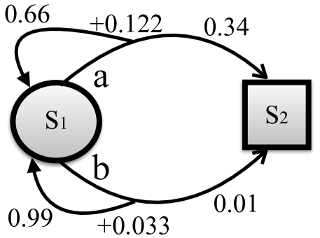
We first show that can lead to problematic behavior. To this end, we ran SARSA with Boltzmann softmax policy (Algorithm 1) on the MDP shown in Figure 1. The edges are labeled with a transition probability (unsigned) and a reward number (signed). Also, state is a terminal state, so we only consider two action values, namely and . Recall that the Boltzmann softmax policy assigns the following probability to each action:
In Figure 2, we plot state–action value estimates at the end of each episode of a single run (smoothed by averaging over ten consecutive points). We set and . The value estimates are unstable.
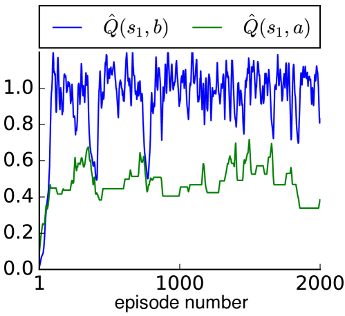
SARSA is known to converge in the tabular setting using -greedy exploration (Littman & Szepesvári, 1996), under decreasing exploration (Singh et al., 2000), and to a region in the function-approximation setting (Gordon, 2001). There are also variants of the SARSA update rule that converge more generally (Perkins & Precup, 2002; Baird & Moore, 1999; Van Seijen et al., 2009). However, this example is the first, to our knowledge, to show that SARSA fails to converge in the tabular setting with Boltzmann policy. The next section provides background for our analysis of the example.
3 Background
A Markov decision process (Puterman, 1994), or MDP, is specified by the tuple , where is the set of states and is the set of actions. The functions and denote the reward and transition dynamics of the MDP. Finally, , the discount rate, determines the relative importance of immediate reward as opposed to the rewards received in the future.
A typical approach to finding a good policy is to estimate how good it is to be in a particular state—the state value function. The value of a particular state given a policy and initial action is written . We define the optimal value of a state–action pair It is possible to define recursively and as a function of the optimal value of the other state–action pairs:
Bellman equations, such as the above, are at the core of many reinforcement-learning algorithms such as Value Iteration (Bellman, 1957). The algorithm computes the value of the best policy in an iterative fashion:
Regardless of its initial value, will converge to .
Littman & Szepesvári (1996) generalized this algorithm by replacing the operator by any arbitrary operator , resulting in the generalized value iteration (GVI) algorithm with the following update rule:
| (1) |
Crucially, convergence of GVI to a unique fixed point follows if operator is a non-expansion with respect to the infinity norm:
for any , and .
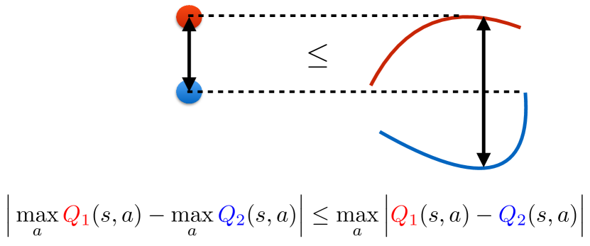
As mentioned earlier, the operator is known to be a non-expansion, as illustrated in Figure 3. mean and operators are also non-expansions. Therefore, each of these operators can play the role of in GVI, resulting in convergence to the corresponding unique fixed point. However, the Boltzmann softmax operator, , is not a non-expansion (Littman, 1996). Note that we can relate GVI to SARSA by observing that SARSA’s update is a stochastic implementation of GVI’s update. Under a Boltzmann softmax policy , the target of the (expected) SARSA update is the following:
This matches the GVI update (1) when .
4 Boltzmann Has Multiple Fixed Points
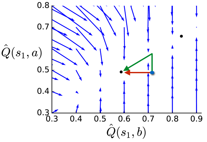
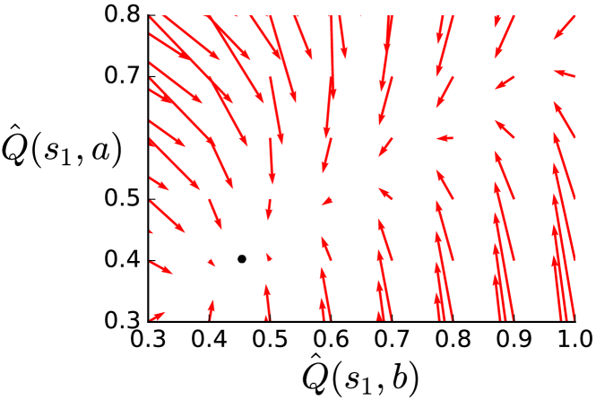
Although it has been known for a long time that the Boltzmann operator is not a non-expansion (Littman, 1996), we are not aware of a published example of an MDP for which two distinct fixed points exist. The MDP presented in Figure 1 is the first example where, as shown in Figure 4, GVI under has two distinct fixed points. We also show, in Figure 5, a vector field visualizing GVI updates under . The updates can move the current estimates farther from the fixed points. The behavior of SARSA (Figure 2) results from the algorithm stochastically bouncing back and forth between the two fixed points. When the learning algorithm performs a sequence of noisy updates, it moves from a fixed point to the other. As we will show later, planning will also progress extremely slowly near the fixed points. The lack of the non-expansion property leads to multiple fixed points and ultimately a misbehavior in learning and planning.

5 Mellowmax and its Properties
We advocate for an alternative softmax operator defined as follows:
which can be viewed as a particular instantiation of the quasi-arithmetic mean (Beliakov et al., 2016). It can also be derived from information theoretical principles as a way of regularizing policies with a cost function defined by KL divergence (Todorov, 2006; Rubin et al., 2012; Fox et al., 2016). Note that the operator has previously been utilized in other areas, such as power engineering (Safak, 1993).
We show that , which we refer to as mellowmax, has the desired properties and that it compares quite favorably to in practice.
5.1 Mellowmax is a Non-Expansion
We prove that is a non-expansion (Property 2), and therefore, GVI and SARSA under are guaranteed to converge to a unique fixed point.
Let and be two vectors of values. Let for be the difference of the th components of the two vectors. Also, let be the index with the maximum component-wise difference, . For simplicity, we assume that is unique and . Also, without loss of generality, we assume that . It follows that:
allowing us to conclude that mellowmax is a non-expansion under the infinity norm.
5.2 Maximization
Mellowmax includes parameter settings that allow for maximization (Property 1) as well as for minimization. In particular, as goes to infinity, acts like .
Let and let . Note that is the number of maximum values (“winners”) in X. Then:
That is, the operator acts more and more like pure maximization as the value of is increased. Conversely, as goes to , the operator approaches the minimum.
5.3 Derivatives
We can take the derivative of mellowmax with respect to each one of the arguments and for any non-zero :
Note that the operator is non-decreasing in each component of X.
Moreover, we can take the derivative of mellowmax with respect to . We define and . Then:
and so:
ensuring differentiablity of the operator (Property 3).
5.4 Averaging
Because of the division by in the definition of , the parameter cannot be set to zero. However, we can examine the behavior of as approaches zero and show that the operator computes an average in the limit.
Since both the numerator and denominator go to zero as goes to zero, we will use L’Hôpital’s rule and the derivative given in the previous section to derive the value in the limit:
That is, as gets closer to zero, approaches the mean of the values in X.
6 Maximum Entropy Mellowmax Policy
As described, computes a value for a list of numbers somewhere between its minimum and maximum. However, it is often useful to actually provide a probability distribution over the actions such that (1) a non-zero probability mass is assigned to each action, and (2) the resulting expected value equals the computed value. Such a probability distribution can then be used for action selection in algorithms such as SARSA.
In this section, we address the problem of identifying such a probability distribution as a maximum entropy problem—over all distributions that satisfy the properties above, pick the one that maximizes information entropy (Cover & Thomas, 2006; Peters et al., 2010). We formally define the maximum entropy mellowmax policy of a state as:
| (2) | |||
| (6) |
Note that this optimization problem is convex and can be solved reliably using any numerical convex optimization library.
One way of finding the solution, which leads to an interesting policy form, is to use the method of Lagrange multipliers. Here, the Lagrangian is:
Taking the partial derivative of the Lagrangian with respect to each and setting them to zero, we obtain:
These equations, together with the two linear constraints in (2), form equations to constrain the variables and the two Lagrangian multipliers and .
Solving this system of equations, the probability of taking an action under the maximum entropy mellowmax policy has the form:
where is a value for which:
The argument for the existence of a unique root is simple. As the term corresponding to the best action dominates, and so, the function is positive. Conversely, as the term corresponding to the action with lowest utility dominates, and so the function is negative. Finally, by taking the derivative, it is clear that the function is monotonically increasing, allowing us to conclude that there exists only a single root. Therefore, we can find easily using any root-finding algorithm. In particular, we use Brent’s method (Brent, 2013) available in the Numpy library of Python.
This policy has the same form as Boltzmann softmax, but with a parameter whose value depends indirectly on . This mathematical form arose not from the structure of , but from maximizing the entropy. One way to view the use of the mellowmax operator, then, is as a form of Boltzmann policy with a temperature parameter chosen adaptively in each state to ensure that the non-expansion property holds.
Finally, note that the SARSA update under the maximum entropy mellowmax policy could be thought of as a stochastic implementation of the GVI update under the operator:
due to the first constraint of the convex optimization problem (2). Because mellowmax is a non-expansion, SARSA with the maximum entropy mellowmax policy is guaranteed to converge to a unique fixed point. Note also that, similar to other variants of SARSA, the algorithm simply bootstraps using the value of the next state while implementing the new policy.
7 Experiments on MDPs
We observed that in practice computing mellowmax can yield overflow if the exponentiated values are large. In this case, we can safely shift the values by a constant before exponentiating them due to the following equality:
A value of usually avoids overflow.
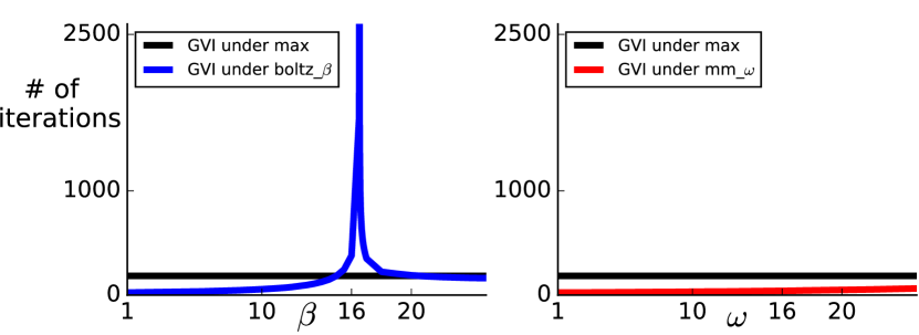
We repeat the experiment from Figure 5 for mellowmax with to get a vector field. The result, presented in Figure 6, show a rapid and steady convergence towards the unique fixed point. As a result, GVI under can terminate significantly faster than GVI under , as illustrated in Figure 7.
We present three additional experiments. The first experiment investigates the behavior of GVI with the softmax operators on randomly generated MDPs. The second experiment evaluates the softmax policies when used in SARSA with a tabular representation. The last experiment is a policy gradient experiment where a deep neural network, with a softmax output layer, is used to directly represent the policy.
7.1 Random MDPs
The example in Figure 1 was created carefully by hand. It is interesting to know whether such examples are likely to be encountered naturally. To this end, we constructed 200 MDPs as follows: We sampled from and from uniformly at random. We initialized the transition probabilities by sampling uniformly from . We then added to each entry, with probability 0.5, Gaussian noise with mean 1 and variance 0.1. We next added, with probability 0.1, Gaussian noise with mean 100 and variance 1. Finally, we normalized the raw values to ensure that we get a transition matrix. We did a similar process for rewards, with the difference that we divided each entry by the maximum entry and multiplied by 0.5 to ensure that .
We measured the failure rate of GVI under and by stopping GVI when it did not terminate in 1000 iterations. We also computed the average number of iterations needed before termination. A summary of results is presented in the table below. Mellowmax outperforms Boltzmann based on the three measures provided below.
| MDPs, no terminate | MDPs, fixed points | average iterations | |
|---|---|---|---|
| 8 of 200 | 3 of 200 | 231.65 | |
| 0 | 0 | 201.32 |
7.2 Multi-passenger Taxi Domain
We evaluated SARSA on the multi-passenger taxi domain introduced by Dearden et al. (1998). (See Figure 8.)
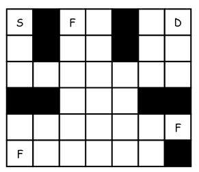
One challenging aspect of this domain is that it admits many locally optimal policies. Exploration needs to be set carefully to avoid either over-exploring or under-exploring the state space. Note also that Boltzmann softmax performs remarkably well on this domain, outperforming sophisticated Bayesian reinforcement-learning algorithms (Dearden et al., 1998).
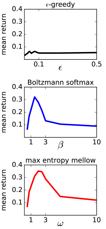
As shown in Figure 9, SARSA with the epsilon-greedy policy performs poorly. In fact, in our experiment, the algorithm rarely was able to deliver all the passengers. However, SARSA with Boltzmann softmax and SARSA with the maximum entropy mellowmax policy achieved significantly higher average reward. Maximum entropy mellowmax policy is no worse than Boltzmann softmax, here, suggesting that the greater stability does not come at the expense of less effective exploration.
7.3 Lunar Lander Domain
In this section, we evaluate the use of the maximum entropy mellowmax policy in the context of a policy-gradient algorithm. Specifically, we represent a policy by a neural network (discussed below) that maps from states to probabilities over actions. A common choice for the activation function of the last layer is the Boltzmann softmax policy. In contrast, we can use maximum entropy mellowmax policy, presented in Section 6, by treating the inputs of the activation function as values.
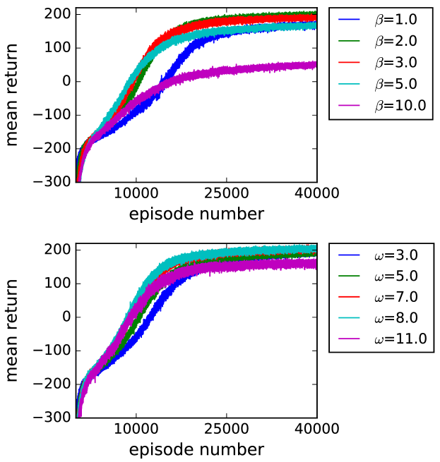
We used the lunar lander domain, from OpenAI Gym (Brockman et al., 2016) as our benchmark. A screenshot of the domain is presented in Figure 10. This domain has a continuous state space with 8 dimensions, namely x-y coordinates, x-y velocities, angle and angular velocities, and leg-touchdown sensors. There are 4 discrete actions to control 3 engines. The reward is +100 for a safe landing in the designated area, and for a crash. There is a small shaping reward for approaching the landing area. Using the engines results in a negative reward. An episode finishes when the spacecraft crashes or lands. Solving the domain is defined as maintaining mean episode return higher than 200 in 100 consecutive episodes.
The policy in our experiment is represented by a neural network with a hidden layer comprised of 16 units with RELU activation functions, followed by a second layer with 16 units and softmax activation functions. We used REINFORCE to train the network. A batch episode size of 10 was used, as we had stability issues with smaller episode batch sizes. We used the Adam algorithm (Kingma & Ba, 2014) with and the other parameters as suggested by the paper. We used Keras (Chollet, 2015) and Theano (Team et al., 2016) to implement the neural network architecture.

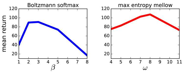
For each softmax policy, we present in Figure 11 the learning curves for different values of their free parameter. We further plot average return over all 40000 episodes. Mellowmax outperforms Boltzmann at its peak.
8 Related Work
Softmax operators play an important role in sequential decision-making algorithms.
In model-free reinforcement learning, they can help strike a balance between exploration (mean) and exploitation (max). Decision rules based on epsilon-greedy and Boltzmann softmax, while very simple, often perform surprisingly well in practice, even outperforming more advanced exploration techniques (Kuleshov & Precup, 2014) that require significant approximation for complex domains. When learning “on policy”, exploration steps can (Rummery & Niranjan, 1994) and perhaps should (John, 1994) become part of the value-estimation process itself. On-policy algorithms like SARSA can be made to converge to optimal behavior in the limit when the exploration rate and the update operator is gradually moved toward (Singh et al., 2000). Our use of softmax in learning updates reflects this point of view and shows that the value-sensitive behavior of Boltzmann exploration can be maintained even as updates are made stable.
Analyses of the behavior of human subjects in choice experiments very frequently use softmax. Sometimes referred to in the literature as logit choice (Stahl & Wilson, 1994), it forms an important part of the most accurate predictor of human decisions in normal-form games (Wright & Leyton-Brown, 2010), quantal level- reasoning (QLk). Softmax-based fixed points play a crucial role in this work. As such, mellowmax could potentially make a good replacement.
Algorithms for inverse reinforcement learning (IRL), the problem of inferring reward functions from observed behavior (Ng & Russell, 2000), frequently use a Boltzmann operator to avoid assigning zero probability to non-optimal actions and hence assessing an observed sequence as impossible. Such methods include Bayesian IRL (Ramachandran & Amir, 2007), natural gradient IRL (Neu & Szepesvári, 2007), and maximum likelihood IRL (Babes et al., 2011). Given the recursive nature of value defined in these problems, mellowmax could be a more stable and efficient choice.
In linearly solvable MDPs (Todorov, 2006), an operator similar to mellowmax emerges when using an alternative characterization for cost of action selection in MDPs. Inspired by this work Fox et al. (2016) introduced an off-policy G-learning algorithm that uses the operator to perform value-function updates. Instead of performing off-policy updates, we introduced a convergent variant of SARSA with Boltzmann policy and a state-dependent temperature parameter. This is in contrast to Fox et al. (2016) where an epsilon greedy behavior policy is used.
9 Conclusion and Future Work
We proposed the mellowmax operator as an alternative to the Boltzmann softmax operator. We showed that mellowmax has several desirable properties and that it works favorably in practice. Arguably, mellowmax could be used in place of Boltzmann throughout reinforcement-learning research.
A future direction is to analyze the fixed point of planning, reinforcement-learning, and game-playing algorithms when using the mellowmax operators. In particular, an interesting analysis could be one that bounds the sub-optimality of the fixed points found by GVI.
An important future work is to expand the scope of our theoretical understanding to the more general function approximation setting, in which the state space or the action space is large and abstraction techniques are used. Note that the importance of non-expansion in the function approximation case is well-established. (Gordon, 1995)
Finally, due to the convexity of mellowmax (Boyd & Vandenberghe, 2004), it is compelling to use it in a gradient-based algorithm in the context of sequential decision making. IRL is a natural candidate given the popularity of softmax in this setting.
10 Acknowledgments
The authors gratefully acknowledge the assistance of George D. Konidaris, as well as anonymous ICML reviewers for their outstanding feedback.
References
- Babes et al. (2011) Babes, Monica, Marivate, Vukosi N., Littman, Michael L., and Subramanian, Kaushik. Apprenticeship learning about multiple intentions. In International Conference on Machine Learning, pp. 897–904, 2011.
- Baird & Moore (1999) Baird, Leemon and Moore, Andrew W. Gradient descent for general reinforcement learning. In Advances in Neural Information Processing Systems, pp. 968–974, 1999.
- Baker et al. (2007) Baker, Chris L, Tenenbaum, Joshua B, and Saxe, Rebecca R. Goal inference as inverse planning. In Proceedings of the 29th Annual Meeting of the Cognitive Science Society, 2007.
- Beliakov et al. (2016) Beliakov, Gleb, Sola, Humberto Bustince, and Sánchez, Tomasa Calvo. A Practical Guide to Averaging Functions. Springer, 2016.
- Bellman (1957) Bellman, Richard. A Markovian decision process. Journal of Mathematics and Mechanics, 6(5):679–684, 1957.
- Boyd & Vandenberghe (2004) Boyd, S.P. and Vandenberghe, L. Convex optimization. Cambridge University Press, 2004.
- Brent (2013) Brent, Richard P. Algorithms for minimization without derivatives. Courier Corporation, 2013.
- Brockman et al. (2016) Brockman, Greg, Cheung, Vicki, Pettersson, Ludwig, Schneider, Jonas, Schulman, John, Tang, Jie, and Zaremba, Wojciech. Openai gym, 2016.
- Chollet (2015) Chollet, François. Keras. https://github.com/fchollet/keras, 2015.
- Cover & Thomas (2006) Cover, T.M. and Thomas, J.A. Elements of Information Theory. John Wiley and Sons, 2006.
- Dearden et al. (1998) Dearden, Richard, Friedman, Nir, and Russell, Stuart. Bayesian Q-learning. In Fifteenth National Conference on Artificial Intelligence (AAAI), pp. 761–768, 1998.
- Fox et al. (2016) Fox, Roy, Pakman, Ari, and Tishby, Naftali. Taming the noise in reinforcement learning via soft updates. In Proceedings of the Thirty-Second Conference on Uncertainty in Artificial Intelligence, pp. 202–211. AUAI Press, 2016.
- Gordon (1995) Gordon, Geoffrey J. Stable function approximation in dynamic programming. In Proceedings of the twelfth international conference on machine learning, pp. 261–268, 1995.
- Gordon (2001) Gordon, Geoffrey J. Reinforcement learning with function approximation converges to a region, 2001. Unpublished.
- John (1994) John, George H. When the best move isn’t optimal: Q-learning with exploration. In Proceedings of the Twelfth National Conference on Artificial Intelligence, pp. 1464, Seattle, WA, 1994.
- Kingma & Ba (2014) Kingma, Diederik and Ba, Jimmy. Adam: A method for stochastic optimization. arXiv preprint arXiv:1412.6980, 2014.
- Kuleshov & Precup (2014) Kuleshov, Volodymyr and Precup, Doina. Algorithms for multi-armed bandit problems. arXiv preprint arXiv:1402.6028, 2014.
- Littman & Szepesvári (1996) Littman, Michael L. and Szepesvári, Csaba. A generalized reinforcement-learning model: Convergence and applications. In Saitta, Lorenza (ed.), Proceedings of the Thirteenth International Conference on Machine Learning, pp. 310–318, 1996.
- Littman (1996) Littman, Michael Lederman. Algorithms for Sequential Decision Making. PhD thesis, Department of Computer Science, Brown University, February 1996. Also Technical Report CS-96-09.
- Neu & Szepesvári (2007) Neu, Gergely and Szepesvári, Csaba. Apprenticeship learning using inverse reinforcement learning and gradient methods. In UAI, 2007.
- Ng & Russell (2000) Ng, Andrew Y. and Russell, Stuart. Algorithms for inverse reinforcement learning. In International Conference on Machine Learning, pp. 663–670, 2000.
- Perkins & Precup (2002) Perkins, Theodore J and Precup, Doina. A convergent form of approximate policy iteration. In Advances in Neural Information Processing Systems, pp. 1595–1602, 2002.
- Peters et al. (2010) Peters, Jan, Mülling, Katharina, and Altun, Yasemin. Relative entropy policy search. In AAAI. Atlanta, 2010.
- Puterman (1994) Puterman, Martin L. Markov Decision Processes—Discrete Stochastic Dynamic Programming. John Wiley & Sons, Inc., New York, NY, 1994.
- Ramachandran & Amir (2007) Ramachandran, Deepak and Amir, Eyal. Bayesian inverse reinforcement learning. In IJCAI, 2007.
- Rubin et al. (2012) Rubin, Jonathan, Shamir, Ohad, and Tishby, Naftali. Trading value and information in mdps. In Decision Making with Imperfect Decision Makers, pp. 57–74. Springer, 2012.
- Rummery & Niranjan (1994) Rummery, G. A. and Niranjan, M. On-line Q-learning using connectionist systems. Technical Report CUED/F-INFENG/TR 166, Cambridge University Engineering Department, 1994.
- Safak (1993) Safak, Aysel. Statistical analysis of the power sum of multiple correlated log-normal components. IEEE Transactions on Vehicular Technology, 42(1):58–61, 1993.
- Singh et al. (2000) Singh, Satinder, Jaakkola, Tommi, Littman, Michael L., and Szepesvári, Csaba. Convergence results for single-step on-policy reinforcement-learning algorithms. Machine Learning, 39:287–308, 2000.
- Stahl & Wilson (1994) Stahl, Dale O. and Wilson, Paul W. Experimental evidence on players’ models of other players. Journal of Economic Behavior and Organization, 25(3):309––327, 1994.
- Sutton (1990) Sutton, Richard S. Integrated architectures for learning, planning, and reacting based on approximating dynamic programming. In Proceedings of the Seventh International Conference on Machine Learning, pp. 216–224, Austin, TX, 1990. Morgan Kaufmann.
- Sutton & Barto (1998) Sutton, Richard S. and Barto, Andrew G. Reinforcement Learning: An Introduction. The MIT Press, 1998.
- Team et al. (2016) Team, The Theano Development, Al-Rfou, Rami, Alain, Guillaume, Almahairi, Amjad, Angermueller, Christof, Bahdanau, Dzmitry, Ballas, Nicolas, Bastien, Frédéric, Bayer, Justin, Belikov, Anatoly, et al. Theano: A python framework for fast computation of mathematical expressions. arXiv preprint arXiv:1605.02688, 2016.
- Thrun (1992) Thrun, Sebastian B. The role of exploration in learning control. In White, David A. and Sofge, Donald A. (eds.), Handbook of Intelligent Control: Neural, Fuzzy, and Adaptive Approaches, pp. 527–559. Van Nostrand Reinhold, New York, NY, 1992.
- Todorov (2006) Todorov, Emanuel. Linearly-solvable markov decision problems. In NIPS, pp. 1369–1376, 2006.
- Van Seijen et al. (2009) Van Seijen, Harm, Van Hasselt, Hado, Whiteson, Shimon, and Wiering, Marco. A theoretical and empirical analysis of Expected Sarsa. In 2009 IEEE Symposium on Adaptive Dynamic Programming and Reinforcement Learning, pp. 177–184. IEEE, 2009.
- Williams (1992) Williams, Ronald J. Simple statistical gradient-following algorithms for connectionist reinforcement learning. Machine Learning, 8(3):229–256, 1992.
- Wright & Leyton-Brown (2010) Wright, James R. and Leyton-Brown, Kevin. Beyond equilibrium: Predicting human behavior in normal-form games. In AAAI, 2010.