Monte Carlo simulations of the disordered three-color quantum Ashkin-Teller chain

Abstract

We investigate the zero-temperature quantum phase transitions of the disordered three-color quantum Ashkin-Teller spin chain by means of large-scale Monte Carlo simulations. We find that the first-order phase transitions of the clean system are rounded by the quenched disorder. For weak inter-color coupling, the resulting emergent quantum critical point between the paramagnetic phase and the magnetically ordered Baxter phase is of infinite-randomness type and belongs to the universality class of the random transverse-field Ising model, as predicted by recent strong-disorder renormalization group calculations. We also find evidence for unconventional critical behavior in the case of strong inter-color coupling, even though an unequivocal determination of the universality class is beyond our numerical capabilities. We compare our results to earlier simulations, and we discuss implications for the classification of phase transitions in the presence of disorder.

I Introduction

Zero-temperature quantum phase transitions can be classified into continuous or first-order just as classical thermal phase transitions. First-order quantum phase transitions have gained considerable attention recently, not only because of their fundamental interest but also because experimentally important transitions turn from being continuous at higher temperatures to first-order at lower temperatures. A prominent example of this behavior is the itinerant ferromagnetic transition.Belitz et al. (1997); *BelitzKirkpatrickVojta99; Belitz et al. (2005) (For a recent review of metallic quantum ferromagnets see Ref. Brando et al., 2016.)

As real materials always contain a certain amount vacancies, impurities, or other defects, understanding the influence of such quenched disorder is of both conceptual and practical importance. Theoretical research on continuous quantum phase transitions in the presence of disorder has predicted a number of exotic phenomena such as infinite-randomness critical points, Fisher (1992); *Fisher95; Motrunich et al. (2000); Hoyos et al. (2007); *VojtaKotabageHoyos09 quantum Griffiths phases, Thill and Huse (1995); Rieger and Young (1996); *YoungRieger96 and smeared phase transitions. Vojta (2003); *HoyosVojta08 More recently, several of these phenomena have been observed in experiments. Guo et al. (2007); *GYMBHCHD10a; Westerkamp et al. (2009); Ubaid-Kassis et al. (2010); Demkó et al. (2012) A classification of strong-disorder effects was developed in Ref. Vojta and Schmalian, 2005 and refined in Ref. Vojta and Hoyos, 2014, see also Refs. Vojta, 2006; *Vojta10; *Vojta14 for reviews.

In contrast, less is known about first-order quantum phase transitions in the presence of disorder. Greenblatt et al. Greenblatt et al. (2009); *AizenmanGreenblattLebowitz12 proved a quantum version of the classical Aizenman-Wehr theorem Imry and Wortis (1979); Hui and Berker (1989); Aizenman and Wehr (1989) that states that first-order phase transitions cannot exist in disordered systems in $d\leq 2$ space dimensions. (If the disorder breaks a continuous symmetry, the marginal dimension is $d=4$.) This agrees with a few available explicit results: Senthil and Majumdar Senthil and Majumdar (1996) predicted that quenched randomness turns the first-order quantum phase transitions of the quantum Potts and clock chains into infinite-randomness critical points in the random transverse-field Ising universality class. The same was found by Goswami et al. Goswami et al. (2008) for the disordered $N$-color one-dimensional quantum Ashkin-Teller model Fradkin (1984); *Shankar85 in the weak-coupling regime (weak interactions between the colors). In the strong-coupling regime, the critical point between the paramagnetic and Baxter phases is still of infinite-randomness type, but it is predicted to be in a different universality class. Hrahsheh et al. (2012); Barghathi et al. (2015)

All these results were obtained using versions of the strong-disorder renormalization group Igloi and Monthus (2005) which becomes controlled in the limit of infinitely strong disorder. It is therefore highly desirable to verify that the predictions also hold for realistic, weakly or moderately disordered systems. A recent Monte Carlo study of the quantum Ashkin-Teller model Bellafard and Chakravarty (2016) provided evidence for the activated scaling expected at an infinite-randomness critical point. However, the authors could not verify the predicted random transverse-field Ising universality class and suggested that the discrepancy stems, perhaps, from the first-order origin of this transition.

To shed some light onto this question, we map the disordered three-color quantum Ashkin-Teller chain onto a $(1+1)$ dimensional classical Hamiltonian with columnar disorder. We investigate this classical model by means of large-scale Monte Carlo simulations for systems with up to 3.6 million lattice sites (10.8 million spins). In the weak-coupling regime, we find universal critical behavior in the random transverse-field Ising universality class, as predicted by the strong-disorder renormalization group. We also perform exploratory simulations in the strong coupling regime that establish the phase diagram and confirm unconventional activated dynamical scaling. However, because the efficient cluster Monte Carlo algorithms we use in the weak-coupling regime are not valid for strong coupling, we can not quantitatively verify the distinct critical behavior predicted in Refs. Hrahsheh et al., 2012; Barghathi et al., 2015.

The rest of the paper is organized as follows. In Sec. II, we introduce the quantum Ashkin-Teller chain and the mapping onto a classical Hamiltonian. We also summarize the predictions of the strong-disorder renormalization group calculations. Section III is devoted to the Monte Carlo simulations and their results. We conclude in Sec. IV.

II Model and theory

II.1 Quantum Ashkin-Teller chain

The $N$-color quantum Ashkin-Teller chain Grest and Widom (1981); Fradkin (1984); *Shankar85 is a generalization of the original model suggested by Ashkin and Teller many decades ago. Ashkin and Teller (1943) It is made up of $N$ coupled identical transverse-field Ising chains each containing $L$ spins. The quantum Hamiltonian can be expressed as

$$H = -\sum_{\alpha=1}^{N}\sum_{i=1}^{L}{\left(J_{i}\sigma_{\alpha,i}^{z}\sigma_{\alpha,i+1}^{z}+h_{i}\sigma_{\alpha,i}^{x}\right)}$$ (2)

$$-\sum_{\alpha<\beta}^{N}\sum_{i=1}^{L}{\left(K_{i}\sigma_{\alpha,i}^{z}\sigma_{\alpha,i+1}^{z}\sigma_{\beta,i}^{z}\sigma_{\beta,i+1}^{z}+g_{i}\sigma_{\alpha,i}^{x}\sigma_{\beta,i}^{x}\right)}~{}~{}.$$

Here, $\sigma^{x}$ and $\sigma^{z}$ are Pauli matrices describing the spin degrees of freedom. $i$ denotes the lattice sites while $\alpha$ and $\beta$ are color indices. The ratios $\epsilon_{h,i}=g_{i}/h_{i}$ and $\epsilon_{J,i}=K_{i}/J_{i}$ characterize the strengths of the inter-color couplings. In the following, we are interested in the case of positive interactions $J_{i}$, $K_{i}$ and fields $h_{i}$, $g_{i}$. Besides its fundamental interest, different versions of the Ashkin-Teller model have been used to describe absorbed atoms on surfaces Bak et al. (1985), organic magnets, current loops in high-temperature superconductors Aji and Varma (2007, 2009), as well as the elastic response of DNA molecules.Chang et al. (2008)

In the clean quantum Ashkin-Teller chain, the interactions and coupling strengths are uniform in space, $J_{i}\equiv J$, $K_{i}\equiv K$, $h_{i}\equiv h$, and $g_{i}\equiv g$. The bulk phases of this model are easily understood qualitatively. In the weak-coupling regime $\epsilon_{J},\epsilon_{h}\ll 1$, the system is in the paramagnetic phase if the transverse fields are larger than the interactions, $h\gg J$. For $h\ll J$, the system is in the ordered (Baxter) phase in which each color orders ferromagnetically but the relative orientation of different colors is arbitrary. Another phase, the so-called product phase, can appear in the strong coupling regime $\epsilon_{J},\epsilon_{h}\gg 1$. In this phase, products $\sigma_{\alpha,i}^{z}\sigma_{\beta,i}^{z}$ of two spins of different colors develop long-range order while the spins $\sigma_{\alpha,i}^{z}$ themselves remain disordered. For at least three colors, the direct quantum phase transition between the paramagnetic and Baxter phases is known to be of first-order. Grest and Widom (1981); Fradkin (1984); *Shankar85; Ceccatto (1991) The quantum Ashkin-Teller chain is therefore a paradigmatic model for studying the effects of disorder on a first-order quantum phase transition.

Note that the form of the Hamiltonian (2) is invariant under the duality transformation $\sigma_{\alpha,i}^{z}\sigma_{\alpha,i+1}^{z}\to\tilde{\sigma}_{\alpha,i}^{x}$, $\sigma_{\alpha,i}^{x}\to\tilde{\sigma}_{\alpha,i}^{z}\tilde{\sigma}_{\alpha,i+1}^{z}$, $J_{i}\rightleftarrows h_{i}$, and $\epsilon_{J,i}\rightleftarrows\epsilon_{h,i}$, where $\tilde{\sigma}_{\alpha,i}^{x}$ and $\tilde{\sigma}_{\alpha,i}^{z}$ are the dual Pauli matrices Baxter (1982). Self-duality therefore requires that a direct transition between the paramagnetic and Baxter phases (for $\epsilon_{h}=\epsilon_{J}$) must occur exactly at $h=J$.

II.2 Renormalization group predictions

We now briefly summarize the results of several strong-disorder renormalization group calculations for the $N$-color random quantum Ashkin-Teller chain. Goswami et al. Goswami et al. (2008) analyzed the weak-coupling regime and found that the inter-color coupling strengths $\epsilon_{J,i},\epsilon_{h,i}$ renormalize to zero, and the renormalization group flow becomes asymptotically identical to that of the one-dimensional random transverse-field Ising model.Fisher (1992); *Fisher95 More specifically, this happens if all initial (bare) $\epsilon_{J,i}$ and $\epsilon_{h,i}$ are smaller than a critical value

$$\epsilon_{c}(N)=\frac{2N-5}{2N-2}+\sqrt{\left(\frac{2N-5}{2N-2}\right)^{2}+\frac{2}{N-1}}~{}.$$ (3)

(For three colors, $\epsilon_{c}\approx 1.281$.) In the weak-coupling regime, the strong disorder renormalization group thus predicts that the first-order quantum phase transition of the clean chain is rounded to a continuous one, with infinite-randomness critical behavior in the random transverse-field Ising universality class.Fisher (1992); *Fisher95

The strong-coupling regime of the random quantum Ashkin-Teller chain was studied in Refs. Hrahsheh et al., 2012, 2014; Barghathi et al., 2015. Using a different implementation of the strong-disorder renormalization group, these papers demonstrated that the inter-color coupling strengths $\epsilon_{J,i}$ and $\epsilon_{h,i}$ renormalize to infinity if their initial (bare) values are larger than $\epsilon_{c}$. This implies that the four-spin interactions and the two-spin field terms in the Hamiltonian dominate the behavior of the system.

If $\epsilon_{J,i}=\epsilon_{h,i}$, the model is self-dual at the critical point. In this case and for at least three colors, there is still a direct transition between the paramagnetic and Baxter phases, i.e., spins and products order at the same point. This transition occurs at $J_{\rm typ}=h_{\rm typ}$ where $J_{\rm typ}$ and $h_{\rm typ}$ refer to the typical values (geometric means) of the random interactions and fields. The critical behavior of this transition is of infinite randomness type but it is not in the random transverse Ising universality class because products and spins both contribute to observables. Hrahsheh et al. (2012); Barghathi et al. (2015) In the general case, $\epsilon_{J,i}\neq\epsilon_{h,i}$, a product phase can appear between the paramagnetic and Baxter phases (this also happens for two colors, even in the self-dual case). Hrahsheh et al. (2014) The phase transition between the paramagnetic and product phases as well as the transition between the product and Baxter phases are both expected to belong to the random transverse-field Ising universality class.

II.3 Quantum-to-classical mapping

To test the renormalization group predictions by Monte Carlo simulations, we now map the random quantum Ashkin-Teller chain onto a (1+1)-dimensional classical Ashkin-Teller model. This can be done using standard methods, e.g., by writing the partition function as a Feynman path integral in imaginary time (see also Ref. Sachdev, 1999). The resulting classical Hamiltonian reads:

$$H_{cl} = -\sum_{\alpha,i,t}\left(J_{i}^{(s)}S^{\alpha}_{i,t}S^{\alpha}_{i+1,t}+J_{i}^{(t)}S^{\alpha}_{i,t}S^{\alpha}_{i,t+1}\right)$$ (4)

$$-\sum_{\alpha<\beta,i,t}\left(\epsilon_{i}^{(s)}J_{i}^{(s)}S^{\alpha}_{i,t}S^{\alpha}_{i+1,t}S^{\beta}_{i,t}S^{\beta}_{i+1,t}\right)$$

$$-\sum_{\alpha<\beta,i,t}\left(\epsilon_{i}^{(t)}J_{i}^{(t)}S^{\alpha}_{i,t}S^{\alpha}_{i,t+1}S^{\beta}_{i,t}S^{\beta}_{i,t+1}\right)~{}.$$

Here, $S^{\alpha}_{i,t}=\pm 1$ is a classical Ising spin of color $\alpha$ at position $i$ in space and $t$ in (imaginary) time. The classical interactions $J_{i}^{(s)}$, $J_{i}^{(t)}$ and coupling constants $\epsilon_{i}^{(s)}$, $\epsilon_{i}^{(t)}$ as well as the classical temperature $T$ are determined by the parameters of the original quantum Hamiltonian (2). (The classical temperature $T$ does not equal the physical temperature of the quantum system (2) which is encoded in the system size $L_{t}$ in time direction.) As we are interested in the critical behavior which is expected to be universal, the precise values of $J_{i}^{(s)}$, $J_{i}^{(t)}$, $\epsilon_{i}^{(s)}$, and $\epsilon_{i}^{(t)}$ are not important and can be chosen for computational convenience (see Sec. III).

We note that the quantum-to-classical mapping generates further terms in the classical Hamiltonian in addition to those shown in (4). These extra terms contain higher products of up to $N$ colors. Neglecting them does not change the critical behavior, but it destroys the self-duality of the Hamiltonian.

III Monte Carlo simulations

III.1 Overview

We perform large-scale Monte Carlo simulations of the classical Hamiltonian (4) for the case of $N=3$ colors by employing an Ising embedding method similar that used in Ref. Wiseman and Domany, 1995. It can be understood as follows. If we fix the values of all spins with color $\alpha\neq 1$, the Hamiltonian (4) acts as an (1+1)-dimensional Ising model for the spins $S^{(1)}_{i,t}$ with effective interaction $J_{ij}^{\textrm{eff}}=J+\epsilon J(S_{i}^{(2)}S_{j}^{(2)}+S_{i}^{(3)}S_{j}^{(3)})$. This embedded Ising model can be simulated by means of any Ising Monte Carlo algorithm. We use a combination of the efficient Swendsen-Wang multicluster algorithm Swendsen and Wang (1987) and the Wolff single cluster alorithm.Wolff (1989) Analogous embedded Ising models can be constructed for the spins $S^{(2)}_{i,t}$ and $S^{(3)}_{i,t}$, and by performing cluster updates for all three embedded Ising models we arrive at a valid and efficient algorithm for the Ashkin-Teller model.

The Swendsen-Wang and Wolff cluster algorithms require all interactions to be nonnegative, $J^{\textrm{eff}}\geq 0$. This is only guaranteed if the coupling constant $\epsilon$ does not exceed $1/(N-1)=1/2$. For larger $\epsilon$, we perform exploratory simulations using the less efficient Metropolis algorithmMetropolis et al. (1953) as well as the Wang-Landau method. Wang and Landau (2001)

By means of these algorithms, we simulate systems with linear sizes $L=10$ to 60 in space direction and $L_{t}=2$ to 60,000 in (imaginary) time direction, using periodic boundary conditions. The largest system had 3.6 million lattice sites, i.e., 10.8 million spins. To implement the quenched disorder, we consider $J_{i}^{(s)}$ and $J_{i}^{(t)}$ to be independent random variables drawn from a binary probability distribution

$$W(J)=c\delta(J-J_{h})+(1-c)\delta(J-J_{l})$$ (5)

where $c$ is the concentration of the higher value $J_{h}$ of the interaction while $1-c$ is the concentration of the lower value $J_{l}$. The couplings are uniform, $\epsilon_{i}^{(s)}=\epsilon_{i}^{(t)}=\epsilon$. As $J_{i}^{(s)}$ and $J_{i}^{(t)}$ only depend on the space coordinate $i$ but not on the time coordinate $t$, the resulting disorder is columnar, i.e., perfectly correlated in the time direction. In the simulations, we use $J_{h}=1$, $J_{l}=0.25$, and $c=0.5$ while $\epsilon$ takes values between 0 and 5. All observables are averaged over 10,000 to 40,000 disorder configurations, unless otherwise noted.

When using cluster algorithms ($\epsilon\leq 0.5$), we equilibrate each sample using 100 full Monte Carlo sweeps. Each full sweep is made up of a Wolff sweep for each color (consisting of a number of single-cluster flips such that the total number of flipped spins equals the number of lattice sites) and a Swendsen-Wang sweep for each color. The Swendsen-Wang sweep aims at equilibrating small clusters of weakly coupled sites that may be missed by the Wolff algorithm. The actual equilibration is significantly faster than 100 sweeps. Zhu et al. (2015) The measurement period consists of another 100 full Monte Carlo sweeps with a measurement taken after each sweep. To deal with biases introduced by using such short measurement periods, we employ improved estimators. Zhu et al. (2015) Simulations for $\epsilon>0.5$ that use the Metropolis and Wang-Landau methods require much longer runs, details will be discussed below.

During the simulation runs, we measure the following observables: energy, specific heat, total magnetization

$$m=\frac{1}{3LL_{t}}\sum_{\alpha}\left|\sum_{i,t}S_{i,t}^{\alpha}\right|$$ (6)

and its susceptibility $\chi_{m}$. A particularly useful quantity for the finite-size scaling analysis is the Binder cumulant

$$g_{\textrm{av}}=\left[1-\frac{\langle m^{4}\rangle}{3\langle m^{2}\rangle^{2}}\right]_{\textrm{dis}}$$ (7)

where $\langle\ldots\rangle$ denotes the thermodynamic (Monte Carlo) average and $[\ldots]_{\textrm{dis}}$ is the disorder average. In addition, we also measure the product order parameter

$$p=\frac{1}{3LL_{t}}\sum_{\alpha<\beta}\left|\sum_{i,t}S_{i,t}^{\alpha}S_{i,t}^{\beta}\right|~{},$$ (8)

the corresponding product susceptibility $\chi_{p}$, and the product Binder cumulant $g_{p}$.

The phase diagram of the classical Hamiltonian (4) resulting from these simulations is shown in Fig. 1.

Figure 1: (Color online) Phase diagram of the classical Hamiltonian (4) for $N=3$ colors and disorder distribution (5) with $J_{h}=1$, $J_{l}=0.25$, and $c=0.5$. The dots and triangles mark the numerically determined transitions between the Baxter, product, and paramagnetic phases. The solid lines are guides to the eye only. The dashed line marks $\epsilon_{c}=1.281$ [see Eq.  (3)] which separates the weak and strong coupling regimes in the strong-disorder renormalization group calculations.

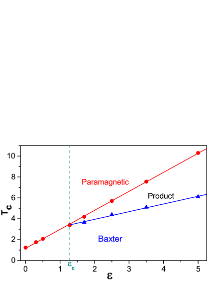
In the weak-coupling regime, $\epsilon<\epsilon_{c}$, we find a direct transition between the magnetically ordered Baxter phase at low temperatures and the paramagnetic high-temperature phase. For strong coupling, $\epsilon>\epsilon_{c}$, these two phases are separated by a product phase. In the following, we study the critical behaviors of the transitions separating these phases in detail, and we compare them to the renormalization group predictions.

III.2 Weak coupling regime

In the weak-coupling regime, $\epsilon<\epsilon_{c}$, we perform simulations for coupling strengths $\epsilon=0$, 0.3 and 0.5 employing the Wolff and Swendsen-Wang cluster algorithms as discussed above. Because the disorder breaks the symmetry between the space and (imaginary) time directions in the Hamiltonian (4), the finite-size scaling analysis of the data to find the critical exponents becomes more complicated. This is caused by the fact that the system sizes $L$ and $L_{t}$ in the space and time directions are expected to have different scaling behavior. Thus, the correct aspect ratios $L_{t}/L$ of the samples to be used in the simulations are not known a priori.

To overcome this problem we follow the iterative method employed in Refs. Guo et al., 1994; Rieger and Young, 1994; Sknepnek et al., 2004; *VojtaSknepnek06; Vojta et al., 2016 which is based on the Binder cumulant. As the renormalization group calculations predict infinite-randomness criticality with activated dynamical scaling, the scaling form of the Binder cumulant (which has scale dimension 0) reads

$$g_{\textrm{av}}(r,L,L_{t})=X_{g}(rL^{1/\nu},\ln(L_{t}/L_{t}^{0})/L^{\psi})~{}.$$ (9)

Here $r=(T-Tc)/T_{c}$ denotes the distance from criticality, $X_{g}$ is a scaling function, and $\psi$ and $\nu$ refer to the tunneling and correlation length critical exponents. $L_{t}^{0}$ is a microscopic reference scale. (For conventional power-law scaling, the second argument of the scaling function would read $L_{t}/L^{z}$ with $z$ being the dynamical exponent.) For fixed $L$, $g_{\rm av}$ has a maximum as function of $L_{t}$ at position $L_{t}^{\rm max}$ and value $g_{\rm av}^{\rm max}$. The position of the maximum yields the optimal sample shape for which the system sizes $L$ and $L_{t}$ behave as the correlation lengths $\xi$ and $\xi_{t}$. At criticality $L_{t}$ must thus behave as $\ln(L_{t}^{\rm max}/L_{t}^{0})\sim L^{\psi}$, fixing the second argument of the scaling function $X_{g}$. Consequently, the peak value $g_{\rm av}^{\rm max}$ is independent of $L$ at criticality, and the $g_{\rm av}$ vs. $r$ curves of optimally shaped samples cross at $T=T_{c}$. Once the optimal sample shapes are found, finite-size scaling proceeds as usual. Barber (1983); Cardy (1988)

To test our simulation and data analysis technique, we first consider the case $\epsilon=0$ for which the quantum Ashkin-Teller model reduces to three decoupled random transverse-field Ising chains whose quantum phase transition is well understood.Fisher (1992); *Fisher95 We perform simulations for sizes $L=10$ to 50 and $L_{t}=2$ to 20000 and find a critical temperature $T_{c}\approx 1.24$. At this temperature, we confirm the activated scaling (9) of the Binder cumulant with the expected value $\psi=1/2$. We also confirm the scaling of the magnetization at $T_{c}$ (for the optimally shaped samples), $m\sim L^{-\beta/\nu}$ with $\beta=0.382$ and $\nu=2$.

After this successful test, we now turn to the Ashkin-Teller model proper. We perform two sets of simulations: (i) $\epsilon=0.5$ using system sizes $L=10$ to 60, $L_{t}=2$ to 60000 and (ii) $\epsilon=0.3$ with system sizes $L=10$ to 50, $L_{t}=2$ to 40000. In each case, we start from a guess for the optimal shapes and find an approximate value of $T_{c}$ from the crossing of the $g_{\rm av}$ vs. $T$ curves for different $L$. We then find the maxima of the $g_{\rm av}$ vs. $L_{t}$ curves at this temperature which yield improved optimal shapes. After iterating this procedure two or three times, we obtain $T_{c}$ and the optimal shapes with reasonable precision.

Figure 2 shows the resulting Binder cumulant $g_{\textrm{av}}$ for $\epsilon=0.5$ as function of $L_{t}$ for different $L$ at the approximate critical temperature of $T_{c}=2.08(5)$.

Figure 2: (Color online) Binder cumulant $g_{\rm av}$ as a function of $L_{t}$ for several $L$ at the critical temperature $T_{c}=2.08$ for $\epsilon=0.5$. The statistical error of $g_{\rm av}$ is smaller than the symbol size.

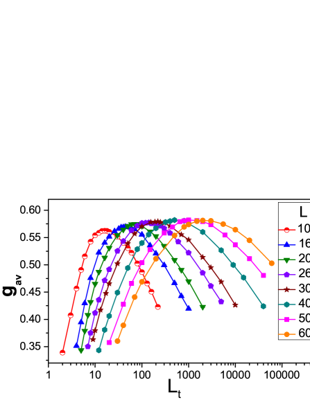
As expected at $T_{c}$, the maxima $g_{\rm av}^{\rm max}$ of these curves are independent of $L$ (the slightly lower values at the smallest $L$ can be attributed to corrections to scaling). Moreover, the figure shows that the $g_{\rm av}$ vs. $L_{t}$ domes rapidly become broader with increasing spatial size $L$, indicating non-power-law scaling. To analyze this quantitatively, we present a scaling plot of these data in Fig. 3.

Figure 3: (Color online) Scaling plot of the Binder cumulant at $T_{c}=2.08$ for $\epsilon=0.5$. The symbols are the same as in Fig. 2 Main panel: Activated scaling $g_{\rm av}/g_{\rm av}^{\rm max}$ vs.  $\ln(L_{t}/L_{t}^{0})/\ln(L_{t}^{\rm max}/L_{t}^{0})$ according to Eq. (9). The microscopic scale $L_{t}^{0}=0.06$. Inset: Power-law scaling $g_{\rm av}/g_{\rm av}^{\rm max}$ vs. $L_{t}/L_{t}^{\rm max}$.

For conventional power-law dynamical scaling, the curves for different $L$ should collapse onto each other when plotted as $g_{\rm av}$ vs. $L_{t}/L_{t}^{\rm max}$. The inset of Fig. 3 clearly demonstrates that this is not the case. In contrast, the Binder cumulant scales well when plotted versus $\ln(L_{t}/L_{t}^{0})/\ln(L_{t}^{\rm max}/L_{t}^{0})$ as shown in the main panel of the figure. (Here, we treat the microscopic scale $L_{t}^{0}$ as a fit parameter). This behavior is in agreement with the activated scaling form (9).

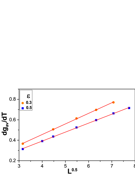
We perform the same analysis for $\epsilon=0.3$ at the approximate critical temperature of $T_{c}=1.76(3)$, with analogous results. To verify the value of the tunneling exponent $\psi$, we now analyze the dependence of $L_{t}^{\rm max}$ on $L$. Figure 4 shows that the data for both $\epsilon=0.3$ and 0.5 can be well fitted with the relation $\ln(L_{t}^{\rm max}/L_{t}^{0})\sim L^{\psi}$ with $\psi=1/2$ as predicted by the strong-disorder renormalization group.

Figure 4: (Color online) $\ln(L_{t}^{\rm max}/L_{t}^{0})$ vs. $L^{0.5}$ at criticality for $\epsilon=0.3$ and 0.5. The data for $\epsilon=0.3$ are shifted upwards by 0.3 for clarity. The solid lines are linear fits. Inset: Double logarithmic plot of $L_{t}^{\rm max}$ vs. $L$.

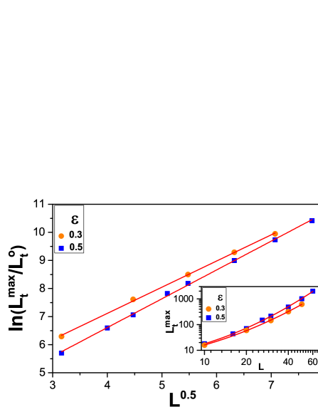
The inset of this figure clearly demonstrates that the relation between $L_{t}^{\rm max}$ and $L$ cannot be described by a power law. We can define, however, an effective (scale-dependent) dynamical exponent $z_{\rm eff}=d\ln(L_{t}^{\rm max})/d\ln(L)$. For $\epsilon=0.5$, it increases from about 2 for the smallest system sizes to almost 4 for the largest ones.

We now turn to the critical behavior of magnetization and susceptibility. At the critical temperature, the magnetization of the optimally shaped samples is predicted to show a power-law dependence on the spatial system size, $m\sim L^{-\beta/\nu}$ with $\beta=2-\phi\approx 0.382$ and $\nu=2$. Here, $\phi=(\sqrt{5}+1)/2$ is the golden mean. In the left panel of Fig. 5, we therefore present a double logarithmic plot of $m$ vs. $L$ for $\epsilon=0.3$ and 0.5.

Figure 5: (Color online) Left: Double logarithmic plot of $m$ vs. $L$ for optimally shaped samples at criticality for $\epsilon=0.3$ and 0.5. The solid lines are fits to the predicted power-law $m\sim L^{-\beta/\nu}$ with $\beta/\nu=0.191$. Right: $\chi/L_{t}$ vs. $[\ln(L_{t}/L_{t}^{0})]^{2\phi-2}$ for optimally shaped samples at criticality for $\epsilon=0.3$ and 0.5. The solid lines are linear fits. The statistical errors of the data in both panels are smaller than the symbol size.

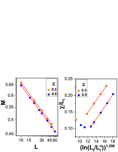
The data for both coupling strengths can be fitted well with the predicted power law. While the magnetization follows a conventional power law dependence on the system size, the susceptibility is affected by the activated scaling. Its predicted system size dependence at criticality can be expressed in terms of the temporal size $L_{t}$ as $\chi\sim L_{t}[\ln(L_{t}/L_{t}^{0})]^{2\phi-2}$. We test this prediction in the right panel of Fig. 5 by plotting $\chi/L_{t}$ vs. $[\ln(L_{t}/L_{t}^{0})]^{2\phi-2}$ for the optimally shaped samples. As the leading power law is divided out, this plot provides a sensitive test of the logarithmic corrections. The figure shows that the susceptibility indeed follows the predicted $L_{t}$ dependence for system sizes $L>20$. The deviations for the smaller sizes can likely be attributed to corrections to scaling stemming from the crossover between the clean first-order phase transition and the infinite-randomness critical point that governs the asymptotic behavior. The clean first-order phase transition is stronger for $\epsilon=0.5$ than for 0.3; accordingly, $\chi$ shows stronger corrections to scaling for $\epsilon=0.5$.

Finally, we analyze the slope $dg_{\rm av}/dT$ of the Binder cumulant at criticality. It is expected to vary with system size as $dg_{\rm av}/dT\sim L^{1/\nu}$ with $\nu=2$. As is shown in Fig. 6, our slopes indeed follow the power-law dependence predicted by the strong-disorder renormalization group for both coupling strengths, $\epsilon=0.3$ and 0.5.

Figure 6: (Color online) Slope $dg_{\rm av}/dT$ of the Binder cumulant vs. $L^{0.5}$ at the critical temperature for $\epsilon=0.3$ and 0.5. The solid lines are linear fits.

III.3 Strong coupling regime

In the strong-coupling regime $\epsilon>\epsilon_{c}\approx 1.281$, we perform simulations for coupling strengths $\epsilon=1.7$, 2.5, 3.5, and 5. These simulations greatly suffer from the fact that the embedded Wolff and Swendsen-Wang cluster algorithms are not valid for $\epsilon>0.5$. We are thus forced to employ the Metropolis single-spin algorithm. In this algorithm, the required equilibration and measurement times increase significantly with system size, reaching several hundred thousand sweeps for moderately large lattices. This severely limits the available sizes and the accuracy of the results. For comparison, we also perform Wang-Landau simulations but the available system sizes are restricted as well.

As the classical Hamiltonian (4) is not self-dual, we can expect a product phase to appear for $\epsilon>\epsilon_{c}$. Indeed, for all studied $\epsilon$ values, we find two distinct phase transitions. (This can already be seen from the specific heat data shown in the left panel of Fig. 7.)

Figure 7: (Color online) Left: Specific heat $C$ vs. classical temperature $T$ for $\epsilon=3.5$, system sizes $L=10$, $L_{t}=100$ and 5000 disorder configurations (using 140,000 Monte Carlo sweeps). Notice two distinct peaks corresponding to two separate phase transitions. Right: Binder cumulant $g_{\rm av}$ as a function of $L_{t}$ for several $L$ at the critical temperature $T_{c}=3.65$ for $\epsilon=1.7$.

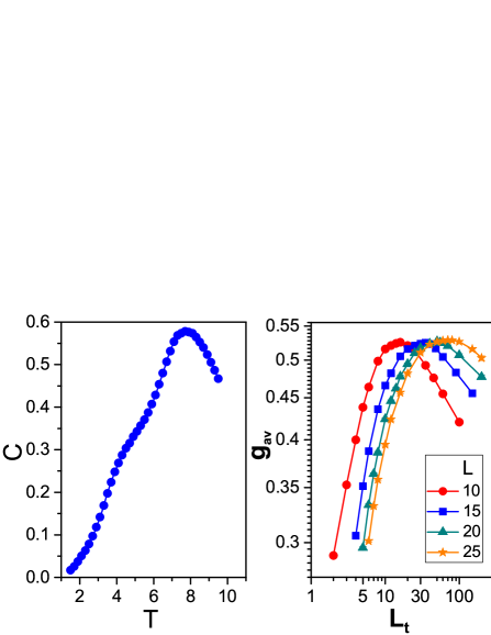
The product order parameter $p$, Eq. (8), develops at a higher temperature $T_{c}^{p}$ while the magnetization becomes nonzero only below a lower temperature $T_{c}^{m}$ (see phase diagram in Fig. 1). In the following, we look at these two transitions separately.

To analyze the transition between the product and Baxter phases (at which the magnetization becomes critical), we use the same procedure based on the Binder cumulant $g_{\rm av}$ as in Sec. III.2. The right panel of Fig. 7 shows the Binder cumulant at the estimated critical temperature $T_{c}^{m}=3.65$ for $\epsilon=1.7$ as a function of $L_{t}$ for several $L$ between 10 and 25. As expected at criticality, the maximum value for each of the curves does not depend on $L$. The figure also shows that the domes become broader with increasing $L$, indicating non-power-law scaling. The largest spatial system size, $L=25$ requires an enormous numerical effort, we averaged over 20,000 disorder configurations each using 700,000 Monte Carlo sweeps. Nonetheless the Binder cumulant at the right end of the dome ($L_{t}=200$) is not fully equilibrated as its value shifts with increasing number of sweeps. Because of the limited system size range and the equilibration problems for the larger sizes we are not able to quantitatively analyze the critical behavior of this transition.

Similar problems, though slightly less severe, also plague the transition between the paramagnetic and product phases at which the product order parameter $p$ becomes critical. Figure 8 shows the Binder cumulant $g_{p}$ for the product order parameter at the estimated critical temperature $T_{c}^{p}=7.55$ and $\epsilon=3.5$ as a function of $L_{t}$.

Figure 8: (Color online) Product Binder cumulant $g_{p}$ as a function of $L_{t}$ for several $L$ at the critical temperature $T_{c}^{p}=7.55$ for $\epsilon=3.5$.

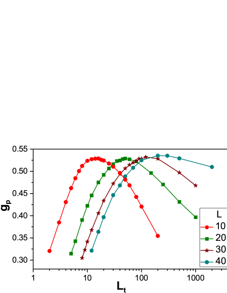
The maxima of the different curves are again independent of $L$, as expected at the critical temperature. Moreover, the domes broaden with increasing system size. A scaling analysis of these data is presented in Fig. 9.

Figure 9: (Color online) Scaling plot of the product Binder cumulant $g_{p}$ at $T_{c}^{p}=7.55$ for $\epsilon=3.5$. The symbols are the same as in Fig. 8 Main panel: Activated scaling $g_{p}/g_{p}^{\rm max}$ vs.  $\ln(L_{t}/L_{t}^{0})/\ln(L_{t}^{\rm max}/L_{t}^{0})$ with $L_{t}^{0}=0.02$. Inset: Power-law scaling $g_{p}/g_{p}^{\rm max}$ vs. $L_{t}/L_{t}^{\rm max}$.

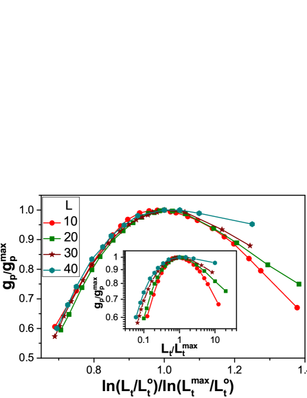
The inset shows that the behavior of $g_{p}$ is not compatible with conventional power-law scaling. In contrast, the data scale reasonably well when plotted versus $\ln(L_{t}/L_{t}^{0})/\ln(L_{t}^{\rm max}/L_{t}^{0})$ as shown in the main panel of the figure. This behavior is in agreement with activated scaling in analogy to Eq. (9) for the Binder cumulant $g_{\rm av}$ of the magnetization. The deviations from data collapse for large $L_{t}$ (ie., at the right side of the domes) stem from the fact that these systems do not equilibrate properly despite us using up to 500,000 Monte Carlo sweeps for each of the 20,000 disorder configurations (the $g_{p}$ values still drift with increasing number of sweeps). This also prevents us from studying larger system sizes.

If we ignore the small system size range and the equilibration problems and analyze (along the lines of Sec. III.2) the system size dependencies of $L_{t}^{\rm max}$, the product order parameter $p$, and its susceptibility $\chi_{p}$, we obtain critical exponents that are roughly compatible with the random transverse-field Ising universality class (as expected from the strong-disorder renormalization group). We do not believe, however, that this constitutes a quantitative confirmation, and we cannot rule out a different universality class with somewhat different critical exponents.

IV Conclusions

In summary, we have studied the fate of the first-order quantum phase transition in the three-color quantum Ashkin-Teller spin chain under the influence of quenched disorder. To this end, we have mapped the random quantum Ashkin-Teller Hamiltonian onto a $(1+1)$-dimensional classical Ashkin-Teller model with columnar disorder. We have then performed large-scale Monte Carlo simulations for systems with up to 3.6 million lattice sites (10.8 million spins). In agreement with the quantum version of the Aizenman-Wehr theorem, we have found that the first-order transition of the clean system is rounded to a continuous one in the presence of bond randomness.

For weak inter-color coupling $\epsilon$, efficient cluster Monte Carlo algorithms have allowed us to simulate large systems. Our data for the quantum phase transition are in full agreement with the results of the strong-disorder renormalization group calculation Goswami et al. (2008) that predicts universal critical behavior in the random transverse-field Ising universality class. Specifically, we have confirmed for two different values of $\epsilon$ the activated dynamical scaling with a tunneling exponent $\psi=1/2$, the correlation length exponent $\nu=2$, and the order parameter exponent $\beta=2-\phi$ with $\phi$ the golden mean. We have also confirmed the behavior of the magnetic susceptibility.

In contrast, our simulations for large inter-color coupling $\epsilon$ have been restricted to smaller system sizes, and they have suffered from equilibration problems because efficient cluster algorithms are not available. Consequently, we have not been able to fully test the renormalization group calculations in this regime. Our numerical data provide evidence for activated dynamical scaling at the quantum phase transitions between the paramagnetic and product phases as well as between the product and Baxter phases. For the latter transition we have also determined rough estimates of the critical exponents and found them compatible with the random transverse-field Ising universality class. However, a quantitative verification of the critical behavior is beyond our current numerical capabilities.

Let us compare our results with earlier simulations. While our critical behavior (in the weak-coupling regime) fully agrees with the random transverse-field Ising universality class, some exponents calculated in Ref. Bellafard and Chakravarty, 2016 show sizable deviations. This is particularly interesting because the spatial system sizes $L$ used in both simulations are comparable (the largest $L$ in Ref. Bellafard and Chakravarty, 2016 is actually larger than ours). We believe that the results of Ref. Bellafard and Chakravarty, 2016 do not agree with the renormalization group predictions because the simulations are still crossing over from the clean first-order transition to the disordered critical point, probably because the chosen parameters lead to relatively weak disorder. This would mean that the measured exponent values are effective rather than true asymptotic exponents. Support for this hypothesis can be obtained from comparing the dynamical scaling in the present paper and in Ref. Bellafard and Chakravarty, 2016. An infinite-randomness critical point features activated dynamical scaling, i.e., the temporal system size $L_{t}$ scales exponentially with the spatial size $L$ via $\ln(L_{t})\sim L^{\psi}$. This implies that the conventional dynamical exponent $z=\infty$. The optimal temporal system size (defined, e.g., via the maximum of the Binder cumulant) therefore must increase very rapidly with $L$. Indeed, the inset of Fig. 4 shows that $L_{t}^{\rm max}$ increases from 18 to about 2000 while $L$ varies only from 10 to 60. The corresponding effective (scale-dependent) dynamical exponent $z_{\rm eff}=d\ln(L_{t}^{\rm max})/d\ln(L)$ reaches almost 4 for the largest sizes. In contrast, $L_{t}^{\rm max}$ reaches only 224 for $L=96$ in Ref. Bellafard and Chakravarty, 2016 and $z_{\rm eff}$ stays below 2, placing the system further away from the asymptotic regime $z_{\rm eff}\to\infty$.

To conclude, as our numerical results (in the weak-coupling regime) fully agree with the renormalization group predictions, we have not found any indications that the asymptotic critical behavior of the disordered system “remembers” the first-order origin of the transition. This supports the expectation that the general classification of disordered critical points developed in Refs. Vojta and Schmalian, 2005; Vojta, 2006; Vojta and Hoyos, 2014 also holds for critical points emerging from the rounding of first-order (quantum) phase transitions. However, the crossover from the clean to the disordered behavior is certainly affected by the first-order nature of the clean transition. The breakup length beyond which phase coexistence is destroyed by domain formation increases with decreasing disorder and may exceed the system size. For sufficiently weak disorder, the true asymptotic behavior is then unobservable in both simulations and experiment. This crossover will be even slower in $(2+1)$-dimensional systems because $d=2$ is the marginal dimension for the Aizenman-Wehr theorem, suggesting an exponential dependence of the breakup length on the disorder strength.Binder (1983); Grinstein and Ma (1983)

References

- Belitz et al. (1997) D. Belitz, T. R. Kirkpatrick, and T. Vojta, Phys. Rev. B 55, 9452 (1997).
- Belitz et al. (1999) D. Belitz, T. R. Kirkpatrick, and T. Vojta, Phys. Rev. Lett. 82, 4707 (1999).
- Belitz et al. (2005) D. Belitz, T. R. Kirkpatrick, and T. Vojta, Rev. Mod. Phys. 77, 579 (2005).
- Brando et al. (2016) M. Brando, D. Belitz, F. M. Grosche, and T. R. Kirkpatrick, Rev. Mod. Phys. 88, 025006 (2016).
- Fisher (1992) D. S. Fisher, Phys. Rev. Lett. 69, 534 (1992).
- Fisher (1995) D. S. Fisher, Phys. Rev. B 51, 6411 (1995).
- Motrunich et al. (2000) O. Motrunich, S. C. Mau, D. A. Huse, and D. S. Fisher, Phys. Rev. B 61, 1160 (2000).
- Hoyos et al. (2007) J. A. Hoyos, C. Kotabage, and T. Vojta, Phys. Rev. Lett. 99, 230601 (2007).
- Vojta et al. (2009) T. Vojta, C. Kotabage, and J. A. Hoyos, Phys. Rev. B 79, 024401 (2009).
- Thill and Huse (1995) M. Thill and D. A. Huse, Physica A 214, 321 (1995).
- Rieger and Young (1996) H. Rieger and A. P. Young, Phys. Rev. B 54, 3328 (1996).
- Young and Rieger (1996) A. P. Young and H. Rieger, Phys. Rev. B 53, 8486 (1996).
- Vojta (2003) T. Vojta, Phys. Rev. Lett. 90, 107202 (2003).
- Hoyos and Vojta (2008) J. A. Hoyos and T. Vojta, Phys. Rev. Lett. 100, 240601 (2008).
- Guo et al. (2007) S. Guo, D. P. Young, R. T. Macaluso, D. A. Browne, N. L. Henderson, J. Y. Chan, L. Henry, and J. F. DiTusa, Phys. Rev. Lett. 100, 017209 (2007).
- Guo et al. (2010) S. Guo, D. P. Young, R. T. Macaluso, D. A. Browne, N. L. Henderson, J. Y. Chan, L. L. Henry, and J. F. DiTusa, Phys. Rev. B 81, 144423 (2010).
- Westerkamp et al. (2009) T. Westerkamp, M. Deppe, R. Küchler, M. Brando, C. Geibel, P. Gegenwart, A. P. Pikul, and F. Steglich, Phys. Rev. Lett. 102, 206404 (2009).
- Ubaid-Kassis et al. (2010) S. Ubaid-Kassis, T. Vojta, and A. Schroeder, Phys. Rev. Lett. 104, 066402 (2010).
- Demkó et al. (2012) L. Demkó, S. Bordács, T. Vojta, D. Nozadze, F. Hrahsheh, C. Svoboda, B. Dóra, H. Yamada, M. Kawasaki, Y. Tokura, and I. Kézsmárki, Phys. Rev. Lett. 108, 185701 (2012).
- Vojta and Schmalian (2005) T. Vojta and J. Schmalian, Phys. Rev. B 72, 045438 (2005).
- Vojta and Hoyos (2014) T. Vojta and J. A. Hoyos, Phys. Rev. Lett. 112, 075702 (2014).
- Vojta (2006) T. Vojta, J. Phys. A 39, R143 (2006).
- Vojta (2010) T. Vojta, J. Low Temp. Phys. 161, 299 (2010).
- Vojta (2014) T. Vojta, J. Phys. Conf. Series 529, 012016 (2014).
- Greenblatt et al. (2009) R. L. Greenblatt, M. Aizenman, and J. L. Lebowitz, Phys. Rev. Lett. 103, 197201 (2009).
- Aizenman et al. (2012) M. Aizenman, R. L. Greenblatt, and J. L. Lebowitz, J. Math. Phys. 53, 023301 (2012).
- Imry and Wortis (1979) Y. Imry and M. Wortis, Phys. Rev. B 19, 3580 (1979).
- Hui and Berker (1989) K. Hui and A. N. Berker, Phys. Rev. Lett. 62, 2507 (1989).
- Aizenman and Wehr (1989) M. Aizenman and J. Wehr, Phys. Rev. Lett. 62, 2503 (1989).
- Senthil and Majumdar (1996) T. Senthil and S. N. Majumdar, Phys. Rev. Lett. 76, 3001 (1996).
- Goswami et al. (2008) P. Goswami, D. Schwab, and S. Chakravarty, Phys. Rev. Lett. 100, 015703 (2008).
- Fradkin (1984) E. Fradkin, Phys. Rev. Lett. 53, 1967 (1984).
- Shankar (1985) R. Shankar, Phys. Rev. Lett. 55, 453 (1985).
- Hrahsheh et al. (2012) F. Hrahsheh, J. A. Hoyos, and T. Vojta, Phys. Rev. B 86, 214204 (2012).
- Barghathi et al. (2015) H. Barghathi, F. Hrahsheh, J. A. Hoyos, R. Narayanan, and T. Vojta, Phys. Scr. T165, 014040 (2015).
- Igloi and Monthus (2005) F. Igloi and C. Monthus, Phys. Rep. 412, 277 (2005).
- Bellafard and Chakravarty (2016) A. Bellafard and S. Chakravarty, Phys. Rev. B 94, 094408 (2016).
- Grest and Widom (1981) G. S. Grest and M. Widom, Phys. Rev. B 24, 6508 (1981).
- Ashkin and Teller (1943) J. Ashkin and E. Teller, Phys. Rev. 64, 178 (1943).
- Bak et al. (1985) P. Bak, P. Kleban, W. N. Unertl, J. Ochab, G. Akinci, N. C. Bartelt, and T. L. Einstein, Phys. Rev. Lett. 54, 1539 (1985).
- Aji and Varma (2007) V. Aji and C. M. Varma, Phys. Rev. Lett. 99, 067003 (2007).
- Aji and Varma (2009) V. Aji and C. M. Varma, Phys. Rev. B 79, 184501 (2009).
- Chang et al. (2008) Z. Chang, P. Wang, and Y.-H. Zheng, Commun. Theor. Phys. 49, 525 (2008).
- Ceccatto (1991) H. Ceccatto, J. Phys. A 24, 2829 (1991).
- Baxter (1982) R. Baxter, Exactly Solved Models in Statistical Mechanics (Academic Press, New York, 1982).
- Hrahsheh et al. (2014) F. Hrahsheh, J. A. Hoyos, R. Narayanan, and T. Vojta, Phys. Rev. B 89, 014401 (2014).
- Sachdev (1999) S. Sachdev, Quantum phase transitions (Cambridge University Press, Cambridge, 1999).
- Wiseman and Domany (1995) S. Wiseman and E. Domany, Phys. Rev. E 51, 3074 (1995).
- Swendsen and Wang (1987) R. H. Swendsen and J.-S. Wang, Phys. Rev. Lett. 58, 86 (1987).
- Wolff (1989) U. Wolff, Phys. Rev. Lett. 62, 361 (1989).
- Note (1) Generalizations of the Swendsen-Wang and Wolff algorithms exist for systems with competing interaction, but they turn out be much less efficient Kessler and Bretz (1990); Liang (1992).
- Metropolis et al. (1953) N. Metropolis, A. Rosenbluth, M. Rosenbluth, and A. Teller, J. Chem. Phys. 21, 1087 (1953).
- Wang and Landau (2001) F. Wang and D. P. Landau, Phys. Rev. Lett. 86, 2050 (2001).
- Zhu et al. (2015) Q. Zhu, X. Wan, R. Narayanan, J. A. Hoyos, and T. Vojta, Phys. Rev. B 91, 224201 (2015).
- Guo et al. (1994) M. Guo, R. N. Bhatt, and D. A. Huse, Phys. Rev. Lett. 72, 4137 (1994).
- Rieger and Young (1994) H. Rieger and A. P. Young, Phys. Rev. Lett. 72, 4141 (1994).
- Sknepnek et al. (2004) R. Sknepnek, T. Vojta, and M. Vojta, Phys. Rev. Lett. 93, 097201 (2004).
- Vojta and Sknepnek (2006) T. Vojta and R. Sknepnek, Phys. Rev. B. 74, 094415 (2006).
- Vojta et al. (2016) T. Vojta, J. Crewse, M. Puschmann, D. Arovas, and Y. Kiselev, Phys. Rev. B 94, 134501 (2016).
- Barber (1983) M. N. Barber, in Phase Transitions and Critical Phenomena, Vol. 8, edited by C. Domb and J. L. Lebowitz (Academic, New York, 1983) pp. 145–266.
- Cardy (1988) J. Cardy, ed., Finite-size scaling (North Holland, Amsterdam, 1988).
- Binder (1983) K. Binder, Z. Phys. B 50, 343 (1983).
- Grinstein and Ma (1983) G. Grinstein and S.-k. Ma, Phys. Rev. B 28, 2588 (1983).
- Kessler and Bretz (1990) D. A. Kessler and M. Bretz, Phys. Rev. B 41, 4778 (1990).
- Liang (1992) S. Liang, Phys. Rev. Lett. 69, 2145 (1992).