Error Estimates for the Kernel Gain Function Approximation
in the Feedback Particle Filter

Abstract

This paper is concerned with the analysis of the kernel-based algorithm for gain function approximation in the feedback particle filter. The exact gain function is the solution of a Poisson equation involving a probability-weighted Laplacian. The kernel-based method – introduced in our prior work – allows one to approximate this solution using only particles sampled from the probability distribution. This paper describes new representations and algorithms based on the kernel-based method. Theory surrounding the approximation is improved and a novel formula for the gain function approximation is derived. A procedure for carrying out error analysis of the approximation is introduced. Certain asymptotic estimates for bias and variance are derived for the general nonlinear non-Gaussian case. Comparison with the constant gain function approximation is provided. The results are illustrated with the aid of some numerical experiments.

I Introduction

This paper is concerned with the analysis of the kernel-based algorithm for numerical approximation of the gain function in the feedback particle filter algorithm; cf. [11]. The filter represents a numerical solution of the following continuous-time nonlinear filtering problem:

Signal: $$\,\mathrm{d}X_{t} =a(X_{t})\,\mathrm{d}t+\,\mathrm{d}B_{t},\quad X_{0}\sim p_{0}^{*},$$ (1a)

Observation: $$\,\mathrm{d}Z_{t} =h(X_{t})\,\mathrm{d}t+\,\mathrm{d}W_{t},$$ (1b)

where $X_{t}\in\mathbb{R}^{d}$ is the (hidden) state at time $t$, the initial condition $X_{0}$ has the prior density $p_{0}^{*}$, $Z_{t}\in\mathbb{R}$ is the observation, and $\{B_{t}\}$, $\{W_{t}\}$ are mutually independent standard Wiener processes taking values in $\mathbb{R}^{d}$ and $\mathbb{R}$, respectively. The mappings $a(\cdot):\mathbb{R}^{d}\rightarrow\mathbb{R}^{d}$ and $h(\cdot):\mathbb{R}^{d}\rightarrow\mathbb{R}$ are given $C^{1}$ functions. The goal of the filtering problem is to approximate the posterior distribution of the state $X_{t}$ given the time history of observations (filtration) ${\cal Z}_{t}:=\sigma(Z_{s}:0\leq s\leq t)$.

The feedback particle filter (FPF) is a controlled stochastic differential equation (sde),

FPF:

$$\,\mathrm{d}X^{i}_{t}=a(X^{i}_{t})\,\mathrm{d}t+\,\mathrm{d}B^{i}_{t}+{\sf K}_{t}(X^{i}_{t})\circ(\,\mathrm{d}Z_{t}-\frac{h(X^{i}_{t})+\hat{h}_{t}}{2}\,\mathrm{d}t),\;\;X_{0}^{i}\sim p_{0}^{*},$$

for $i=1,\ldots,N$, where $X_{t}^{i}\in\mathbb{R}^{d}$ is the state of the $i^{\text{th}}$ particle at time $t$, the initial condition $X^{i}_{0}\sim p_{0}^{*}$, $B^{i}_{t}$ is a standard Wiener process, and $\hat{h}_{t}:={\sf E}[h(X_{t}^{i})|\mathcal{Z}_{t}]$. Both $B^{i}_{t}$ and $X^{i}_{0}$ are mutually independent and also independent of $X_{t},Z_{t}$. The $\circ$ indicates that the sde is expressed in its Stratonovich form.

The gain function ${\sf K}_{t}$ is obtained by solving a weighted Poisson equation: For each fixed time $t$, the function $\phi$ is the solution to a Poisson equation,

PDE: $$\begin{aligned} \nabla\cdot(p(x,t)\nabla\phi(x,t))&=-(h(x)-\hat{h})p(x,t),\\ \int\phi(x,t)p(x,t)\,\mathrm{d}x&=0\qquad\text{(zero-mean)},\end{aligned}$$ (2)

where $\nabla$ and $\nabla\cdot$ denote the gradient and the divergence operators, respectively, and $p$ denotes the conditional density of $X_{t}^{i}$ given $\mathcal{Z}_{t}$. In terms of the solution $\phi$, the gain function is given by,

Gain Function: $$\quad{\sf K}_{t}(x) =\nabla\phi(x,t)\,.$$

The gain function ${\sf K}_{t}$ is vector-valued (with dimension $d\times 1$) and it needs to be obtained for each fixed time $t$. For the linear Gaussian case, the gain function is the Kalman gain.

FPF is an exact algorithm: If the initial condition $X^{i}_{0}$ is sampled from the prior $p_{0}^{*}$ then

$${\sf P}[X_{t}\in A\mid{\cal Z}_{t}]={\sf P}[X_{t}^{i}\in A\mid{\cal Z}_{t}],\quad\forall\;A\subset\mathbb{R}^{d},\;\;t>0.$$

In a numerical implementation, a finite number, $N$, of particles is simulated and ${\sf P}[X_{t}^{i}\in A\mid{\cal Z}_{t}]\approx\frac{1}{N}\sum_{i=1}^{N}\text{\rm\large 1}[X^{i}_{t}\in A]$ by the Law of Large Numbers (LLN).

The challenging part in the numerical implementation of the FPF algorithm is the solution of the PDE (2). This has been the subject of a number of recent studies: In our original FPF papers, a Galerkin numerical method was proposed; cf., [13, 14]. A special case of the Galerkin solution is the constant gain approximation formula which is often a popular choice in practice [13, 10, 12, 2]. The main issue with the Galerkin approximation is to choose the basis functions. A proper orthogonal decomposition (POD)-based procedure to select basis functions is introduced in [3] and certain continuation schemes appear in [8]. Apart from the Galerkin procedure, probabilistic approaches based on dynamic programming appear in [9].

In a recent work, we introduced a basis-free kernel-based algorithm for approximating the solution of the gain function [11]. The key step is to construct a Markov matrix on the $N$-node graph defined by the $N$ particles $\{X^{i}_{t}\}_{i=1}^{N}$. The value of the function $\phi$ for the particles, $\phi(X^{i}_{t})$, is then approximated by solving a fixed-point problem involving the Markov matrix. The fixed-point problem is shown to be a contraction and the method of successive approximation applies to numerically obtain the solution.

The present paper presents a continuation and refinement of the analysis for the kernel-based method. The contributions are as follows: A novel formula for the gain function is derived for the kernel-based approximation. A procedure for carrying out error analysis of the approximation is introduced. Certain asymptotic estimates for bias and variance are derived for the general nonlinear non-Gaussian case. Comparison with the constant gain approximation formula are provided. These results are illustrated with the aid of some numerical experiments.

The outline of the remainder of this paper is as follows: The mathematical problem of the gain function approximation together with a summary of known results on this topic appears in Sec. II. The kernel-based algorithm including the novel formula for gain function, referred to as (G2), appears in Sec. III. The main theoretical results of this paper including the bias and variance estimates appear in Sec. IV. Some numerical experiments for the same appear in Sec. V.

Notation. $\mathbb{Z}_{+}$ denotes the set of positive integers and $\mathbb{Z}_{+}^{d}$ is the set of $d$-tuples. For vectors $x,y\in\mathbb{R}^{d}$, the dot product is denoted as $x\cdot y$ and $|x|:=\sqrt{x\cdot x}$. Throughout the paper, it is assumed that the probability measures admit a smooth Lebesgue density. A density for a Gaussian random variable with mean $\mu$ and variance $\Sigma$ is denoted as ${\cal N}(\mu,\Sigma)$. $C^{k}$ is used to denote the space of $k$-times continuously differentiable functions. For a function $f$, $\nabla f=\frac{\partial f}{\partial x_{i}}$ is used to denote the gradient. $L^{2}(\mathbb{R}^{d},\rho)$ is the Hilbert space of square integrable functions on $\mathbb{R}^{d}$ equipped with the inner-product, $\big{<}\phi,\psi\big{>}_{L^{2}}:=\int\phi(x)\psi(x)\rho(x)\,\mathrm{d}x$. The associated norm is denoted as $\|\phi\|^{2}_{2}:=\big{<}\phi,\phi\big{>}$. The space $H^{1}(\mathbb{R}^{d},\rho)$ is the space of square integrable functions $\phi$ whose derivative (defined in the weak sense) is in $L^{2}(\mathbb{R}^{d},\rho)$. For the remainder of this paper, $L^{2}$ and $H^{1}$ is used to denote $L^{2}(\mathbb{R}^{d},\rho)$ and $H^{1}(\mathbb{R}^{d},\rho)$, respectively.

II Preliminaries

II-A Problem Statement

The Poisson equation (2) is expressed as,

PDE $$\begin{aligned} -\Delta_{\rho}\phi&=h-\hat{h},\\ \int\phi\rho\,\mathrm{d}x&=0\qquad\text{(zero-mean)},\end{aligned}$$ (3)

where $\rho$ is a probability density on $\mathbb{R}^{d}$, $\Delta_{\rho}\phi:=\frac{1}{\rho}\nabla\cdot(\rho\nabla\phi)$. The gain function ${\sf K}(x):=\nabla\phi(x)$.

Problem statement: Given $N$ independent samples $\{X^{1},\ldots,X^{i},\ldots,X^{N}\}$ drawn from $\rho$, approximate the gain function $\{{\sf K}(X^{1}),\ldots,{\sf K}(X^{i}),\ldots,{\sf K}(X^{N})\}$. The density $\rho$ is not explicitly known.

The appropriate function space for the solutions of (3) is the co-dimension 1 subspace $L^{2}_{0}:=\{\phi\in L^{2};\int\phi\rho\,\mathrm{d}x=0\}$ and $H^{1}_{0}:=\{\phi\in H^{1};\int\phi\rho\,\mathrm{d}x=0\}$; cf. [7, 13].

II-B Existence-Uniqueness

On multiplying both side of (3) by test function $\psi$, one obtains the weak-form of the PDE:

$$\int\nabla\phi\cdot\nabla\psi\;\rho\,\mathrm{d}x=\int(h-\hat{h})\psi\;\rho\,\mathrm{d}x,\quad\forall\psi\in H^{1}.$$ (4)

The following is assumed throughout the paper:

• Assumption A1: The probability density is of the form $\rho(x)=e^{-V(x)}$ where $V\in C^{2}$ with

  $$\liminf_{x\to\infty}\;\;[-\Delta V(x)+\frac{1}{2}|\nabla V(x)|^{2}]=\infty.$$

• Assumption A2: The function $h,\nabla h\in L^{2}$.

Under the Assumption A1, the density $\rho$ admits a spectral gap (or Poincaré inequality) ([1] Thm 4.6.3), i.e., $\exists\lambda_{1}>0$ such that,

$$\int f^{2}\,\rho\,\mathrm{d}x\leq\frac{1}{\lambda_{1}}\int|\nabla f|^{2}\,\rho\,\mathrm{d}x,\quad\forall f\in H^{1}_{0}.$$

The Poincaré inequality implies the existence and uniqueness of a weak solution to the weighted Poisson equation.

Theorem 1

[Theorem 2.2 in [7]]. Assume (A1)-(A2). Then there exists a unique weak solution $\phi\in H_{0}^{1}(\mathbb{R}^{d};\rho)$ satisfying (4). Moreover, the gain function ${\sf K}=\nabla\phi$ is controlled by the size of the data:

$$\int|{\sf K}|^{2}\;\rho\,\mathrm{d}x\leq\frac{1}{\lambda_{1}}\int|h-\hat{h}|^{2}\;\rho\,\mathrm{d}x.$$

 

There are two special cases where the exact solution can be found:

• Scalar case where the state dimension $d=1$;

• Gaussian case where the density $\rho$ is a Gaussian.

The results for these two special cases appear in the following two subsections.

II-C Exact Solution in the Scalar Case

In the scalar case (where $d=1$), the Poisson equation is:

$$-\frac{1}{\rho(x)}\frac{\,\mathrm{d}}{\,\mathrm{d}x}(\rho(x)\frac{\,\mathrm{d}\phi}{\,\mathrm{d}x}(x))=h-\hat{h}.$$

Integrating twice yields the solution explicitly,

$${\sf K}(x)=\frac{\,\mathrm{d}\phi}{\,\mathrm{d}x}(x) =-\frac{1}{\rho(x)}\int_{-\infty}^{x}\rho(z)(h(z)-\hat{h})\,\mathrm{d}z.$$ (5)

For the particular choice of $\rho$ as the sum of two Gaussians ${\cal N}(-1,\sigma^{2})$ and ${\cal N}(+1,\sigma^{2})$ with $\sigma^{2}=0.2$ and $h(x)=x$, the solution obtained using (5) is depicted in Fig. 1.

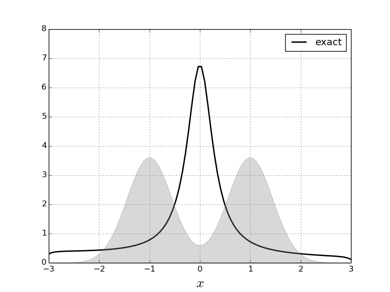
Figure 1: The exact solution to the Poisson equation using the formula (5). The density $\rho$ is the sum of two Gaussians $N(-1,\sigma^{2})$ and $N(+1,\sigma^{2})$, and $h(x)=x$. The density is depicted as the shaded curve in the background.

II-D Exact Spectral Solution for the Gaussian Density

Under Assumption (A1), the spectrum is known to be discrete with an ordered sequence of eigenvalues $0=\lambda_{0}<\lambda_{1}\leq\lambda_{2}\leq\ldots$ and associated eigenfunctions $\{e_{n}\}$ that form a complete orthonormal basis of $L^{2}$ [Corollary 4.10.9 in  [1]]. The trivial eigenvalue $\lambda_{0}=0$ with associated eigenfunction $e_{0}=1$. On the subspace of zero-mean functions, the spectral decomposition yields: For $\phi\in L^{2}_{0}$,

$$-\Delta_{\rho}\phi=\sum_{m=1}^{\infty}\lambda_{m}<e_{m},\phi>e_{m}.$$

The spectral gap condition (II-B) implies that $\lambda_{1}>0$.

The spectral representation (II-D) yields the following closed-form solution of the PDE (3):

$$\phi=\sum_{m=1}^{N}\frac{1}{\lambda_{m}}<e_{m},h-\hat{h}>e_{m}.$$

The spectral representation formula (II-D) is used to obtain the exact solution for the Gaussian case where the eigenvalues and the eigenfunctions are explicitly known in terms of Hermite polynomials.

Definition 1

The Hermite polynomials are recursively defined as

$$\hslash_{n+1}(x)=2\,\hslash_{n}(x)-\hslash^{\prime}_{n}(x),\quad\hslash_{0}(x)=1,$$

where the prime ^′ denotes the derivative.  

Proposition 1

Suppose the density $\rho$ is Gaussian ${\cal}(\mu,\Sigma)$ where the mean $\mu\in\mathbb{R}^{d}$ and the covariance $\Sigma$ is assumed to be a strictly positive definite symmetric matrix. Express $\Sigma=VDV^{T}$ where $D=\text{diag}(\sigma_{1}^{2},\ldots,\sigma_{d}^{2})$ and $V=[V_{1}|\ldots|V_{j}|\ldots|V_{d}]$ is an orthonormal matrix with the $j^{\text{th}}$ column denoted as $V_{j}\in\mathbb{R}^{d}$. For $n=(n_{1},\ldots,n_{d})\in\mathbb{Z}_{+}^{d}$,

• The eigenvalues are,

  $$\lambda_{n}=\sum_{j=1}^{d}\frac{n_{j}}{\sigma_{j}^{2}}.$$

• The corresponding eigenfunctions are,

  $$e_{n}(x)=\prod_{j=1}^{d}\hslash_{n_{j}}(\frac{V_{j}\cdot(x-\mu)}{\sigma_{j}}),$$

  where $\hslash_{n_{j}}$ is the Hermite polynomial.

An immediate corollary is that the first non-zero eigenvalue is $\frac{1}{\sigma_{\text{max}}^{2}}$ and the corresponding eigenfunction is $\psi(x)=V_{\text{max}}\cdot(x-\mu)$, where $\sigma_{\text{max}}^{2}$ is the largest eigenvalue of the covariance matrix and $V_{\text{max}}\in\mathbb{R}^{d}$ is the corresponding eigenvector.

Example 1

Suppose the density $\rho$ is a Gaussian ${\cal}(\mu,\Sigma)$.

• The observation function $h(x)=H\cdot x$, where $H\in\mathbb{R}^{d}$. Then, $\phi=\Sigma H\cdot x$ and the gain function ${\sf K}=\Sigma\,H$ is the Kalman gain.

• Suppose $d=2$, $\mu=[0,0]$, $\Sigma=\begin{bmatrix}\sigma_{1}^{2}&0\\ 0&\sigma_{2}^{2}\end{bmatrix}$, and the observation function $h(x_{1},x_{2})=x_{1}\,x_{2}$. Then,

  $$\phi(x)=\frac{1}{\frac{1}{\sigma_{1}^{2}}+\frac{1}{\sigma_{2}^{2}}}x_{1}x_{2}\quad\text{and}\quad{\sf K}(x_{1},x_{2})=\frac{1}{\frac{1}{\sigma_{1}^{2}}+\frac{1}{\sigma_{2}^{2}}}\begin{bmatrix}x_{2}\\ x_{1}\end{bmatrix}.$$

 

In the general non-Gaussian case, the solution is not known in an explicit form and must be numerically approximated. Note that even in the two exact cases, one may need to numerically approximate the solution because the density is not given in an explicit form. A popular choice is the constant gain approximation briefly described next.

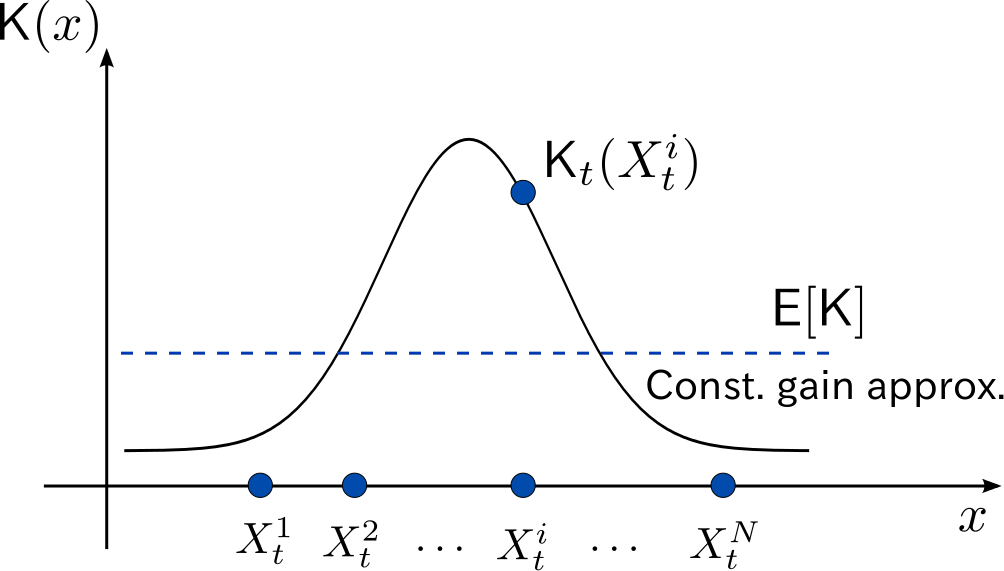
Figure 2: Constant gain approximation: Approximating nonlinear ${\sf K}$ by its expected value ${\sf E}[{\sf K}]$.

II-E Constant gain approximation

The constant gain approximation is the best – in the least-square sense – constant approximation of the gain function (see Fig. 2). Precisely, consider the following least-square optimization problem:

$$\kappa^{\ast}=\arg\min_{\kappa\in\mathbb{R}^{d}}{\sf E}_{\rho}[|{\sf K}-\kappa|^{2}].$$

By using a standard sum of square argument, $\kappa^{\ast}={\sf E}_{\rho}[{\sf K}].$ The expected value admits an explicit formula: In the weak-form (4), choose the test functions to be the coordinate functions: $\psi_{k}(x)=x_{k}$ for $k=1,2,\ldots,d$. Writing $\psi(x)=(\psi_{1},\psi_{2},\ldots,\psi_{d})^{T}=x$,

$$\kappa^{*}={\sf E}_{\rho}[{\sf K}] ={\sf E}_{\rho}[(h-\hat{h})\psi]=\int_{\mathbb{R}^{d}}(h(x)-\hat{h})\;x\;\rho(x)\,\mathrm{d}x.$$

On computing the integral using only the particles, one obtains the formula for the gain function approximation:

$${\sf K}\approx\frac{1}{N}\sum_{i=1}^{N}\;(h(X^{i})-\hat{h}^{(N)})\;X^{i},$$

where $\hat{h}^{(N)}=N^{-1}\sum_{i=1}^{N}h(X^{i})$. This formula is referred to as the constant gain approximation of the gain function; cf., [13]. It is a popular choice in applications [13, 10, 12, 2]..

III Kernel-based Approximation

Semigroup: The spectral gap condition (II-B) implies that $\lambda_{1}>0$. Consequently, the semigroup

$$e^{t\Delta_{\rho}}\phi:=\sum_{m=1}^{\infty}e^{-t\lambda_{m}}<e_{m},\phi>e_{m}$$ (6)

is a strict contraction on the subspace $L^{2}_{0}$. It is also easy to see that $\mu$ is an invariant measure and $\int e^{t\Delta_{\rho}}\phi(x)\,\mathrm{d}\mu(x)=\int\phi(x)\,\mathrm{d}\mu(x)=0$ for all $\phi\in L^{2}_{0}$.

The semigroup formula (6) is used to obtain the solution of the Poisson equation (3) by solving the following fixed-point equation for any fixed positive value of $t$:

$$\phi=e^{t\Delta_{\rho}}\phi+\int_{0}^{t}e^{s\Delta_{\rho}}(h-\hat{h})\,\mathrm{d}s.$$ (7)

A unique solution exists because $e^{t\Delta_{\rho}}$ is a contraction on $L^{2}_{0}$.

Kernel-based method: In the kernel-based algorithm, one approximates the solution of the fixed point problem (7) by approximating the semigroup by an integral operator for $t=\epsilon$. The approximation, introduced in [11], has three main steps:

$$\text{Exact}: \phi =e^{\epsilon\Delta_{\rho}}\phi+\int_{0}^{\epsilon}e^{s\Delta_{\rho}}(h-\hat{h})\,\mathrm{d}s$$ (8)

Kernel approx: $${\phi}_{\epsilon} ={T}_{\epsilon}{\phi}_{\epsilon}+\int_{0}^{\epsilon}T_{s}(h-\hat{h})\,\mathrm{d}s$$ (9)

Empirical approx: $${\phi}^{(N)}_{\epsilon} ={T}^{(N)}_{\epsilon}{\phi}^{(N)}_{\epsilon}+\int_{0}^{\epsilon}T_{s}^{(N)}(h-\hat{h})\,\mathrm{d}s$$ (10)

The justification for these steps is as follows:

• A solution of the Poisson equation (3) is also a solution of the fixed-point problem (8) where $\epsilon>0$ is arbitrary. A unique solution exists because $e^{\epsilon\Delta_{\rho}}$ is contraction on $L^{2}_{0}$.

• The Kernel approximation (9) involves approximating the semigroup $e^{\epsilon\Delta_{\rho}}$ by an integral operator ${T}_{\epsilon}$,

  $${T}_{\epsilon}f:=\int_{\mathbb{R}^{d}}k_{\epsilon}(x,y)f(y)\rho(y)\,\mathrm{d}y$$ (11)

  where the exact form of ${k}_{\epsilon}$ appears in the Appendix, where it is also shown that $e^{\epsilon\Delta_{\rho}}\approx{T}_{\epsilon}$ as $\epsilon\downarrow 0$. The approximation of the semigroup by the integral operator appears in [4, 5].

• The empirical approximation (10) involves approximating the integral operator empirically in terms of the particles,

  $${T}^{(N)}_{\epsilon}f(x):=\frac{1}{N}\sum_{i=1}^{N}{k}_{\epsilon}^{(N)}(x,X^{i})f(X^{i}),$$ (12)

  justified by the LLN.

The gain ${{\sf K}}_{\epsilon}^{(N)}$ is computed by taking the gradient of the fixed-point equation (10). For this purpose, denote,

$$\nabla{T}^{(N)}_{\epsilon}f(x) :=\frac{1}{N}\sum_{j=1}^{N}\nabla{k}_{\epsilon}^{(N)}(x,X^{j})f(X^{j})$$ (13)

$$=\frac{1}{2\epsilon}\bigg{[}\frac{1}{N}\sum_{i=1}^{N}{k}_{\epsilon}^{(N)}(x,X^{i})X^{i}f(X^{i})$$

$$- \left(\frac{1}{N}\sum_{i=1}^{N}{k}_{\epsilon}^{(N)}(x,X^{i})X^{i}\right)\left(\frac{1}{N}\sum_{i=1}^{N}{k}_{\epsilon}^{(N)}(x,X^{i})f(X^{i})\right)\bigg{]}.$$

Next, two approximate formulae for ${{\sf K}}_{\epsilon}^{(N)}$ are presented based on two different approximations of the integral $\int_{0}^{\epsilon}T_{s}^{(N)}(h-\hat{h})\,\mathrm{d}s$:

Approximation 1: The integral term is approximated by $\epsilon(h-\hat{h})$ and the resulting formula for the gain is,

(G1) $$\quad{K}_{\epsilon}^{(N)}(x) :=\nabla{T}^{(N)}_{\epsilon}{\phi}^{(N)}_{\epsilon}(x)+\epsilon\nabla h(x).$$ (14)

By approximating the integral term differently, one can avoid the need to take a derivative of $h$.

Approximation 2: The integral term is approximated by ${T}^{(N)}_{\epsilon}(h-\hat{h})$. The resulting formula for the gain is,

$$(\text{G2}) \quad{K}_{\epsilon}^{(N)}(x) :=\nabla{T}^{(N)}_{\epsilon}{\phi}^{(N)}_{\epsilon}(x)+\epsilon\nabla{T}^{(N)}_{\epsilon}(h-\hat{h})(x).$$ (15)

Remark 1

Although $\nabla{T}^{(N)}_{\epsilon}$ and ${K}_{\epsilon}^{(N)}$ are ultimately important in the numerical algorithm (described next), it is useful to introduce the limiting (as $N\rightarrow\infty$) variables $\nabla{T}_{\epsilon}$ and ${K}_{\epsilon}$. The operator $\nabla{T}_{\epsilon}$ is defined as follows:

$$\nabla{T}_{\epsilon}f(x) =\int_{\mathbb{R}^{d}}\nabla_{x}{k}_{\epsilon}(x,y)f(y)\rho(y)\,\mathrm{d}y$$ (16)

$$=\frac{1}{2\epsilon}\bigg{[}{T}_{\epsilon}(ef)-{T}_{\epsilon}(e){T}_{\epsilon}(f)\bigg{]}(x)$$

where $e$ is the identity function $e(x)=x$.

In terms of $\nabla{T}_{\epsilon}$, the gain function ${K}_{\epsilon}$ is defined by taking of the gradient of the fixed-point equation (9). This leads to the limiting counterpart of the approximation (G1) and (G2). In particular, analogous to (G2),

$${K}_{\epsilon}(x):=\nabla{T}_{\epsilon}{\phi}_{\epsilon}(x)+\epsilon\nabla{T}_{\epsilon}(h-\hat{h})(x),$$

where ${\phi}_{\epsilon}$ is the solution of the fixed-point equation (9).

Numerical Algorithm: A numerical implementation involves the following steps:

• Assemble a $N\times N$ Markov matrix to approximate the finite rank operator ${T}^{(N)}_{\epsilon}$ in (12). The $(i,j)$-entry of the matrix is given by,

  $${\bf T}_{ij}=\frac{1}{N}\sum_{j=1}^{N}{k}_{\epsilon}^{(N)}(X^{i},X^{j}).$$

• Use the method of successive approximation to solve the discrete counterpart of the fixed-point equation (10),

  $$\Phi={\bf T}\Phi+\epsilon({\bf h}-\hat{h}^{(N)})$$ (17)

  where $\Phi:=[{\phi}^{(N)}_{\epsilon}(X^{1}),\ldots,{\phi}^{(N)}_{\epsilon}(X^{N})]\in\mathbb{R}^{N}$ is the (unknown) solution, ${\bf h}:=[h(X^{1}),\ldots,h(X^{N})]\in\mathbb{R}^{N}$ is given, and $\hat{h}^{(N)}=\frac{1}{N}\sum_{i=1}^{N}h(X^{i})$. In filtering applications, the solution from the previous time-step is typically used to initialize the algorithm.

• Once $\Phi$ has been computed, the gain function $\{{\sf K}(X^{1}),\ldots,{\sf K}(X^{i}),\ldots,{\sf K}(X^{N})\}$ is obtained by using either (G1) or (G2). Note that the discrete counterpart of $\nabla{T}^{(N)}_{\epsilon}$ is obtained using the Markov matrix ${\bf T}$.

The overall algorithm is tabulated as Algorithm 1 where (G2) is used for the gain function approximation.

Algorithm 1 Kernel-based gain function approximation

0:  $\{X^{i}\}_{i=1}^{N}$, $H:=\{h(X^{i})\}_{i=1}^{N}$,$\Phi_{0}:=\{\phi_{0}(X^{i})\}_{i=1}^{N}$

0:  $\Phi:=\{\phi(X^{i})\}_{i=1}^{N}$, $\{\nabla\phi(X^{i})\}_{i=1}^{N}$

  Calculate $g_{ij}:=\exp(-|X^{i}-X^{j}|^{2}/4\epsilon)$ for $i,j=1$ to $N$.

  Calculate $k_{ij}:=\frac{g_{ij}}{\sqrt{\sum_{l}g_{il}}\sqrt{\sum_{l}g_{jl}}}$ for $i,j=1$ to $N$.

  Calculate $T_{ij}:=\frac{k_{ij}}{\sum_{l}k_{il}}$ for $i,j=1$ to $N$.

  Calculate $\hat{h}^{(N)}=\frac{1}{N}\sum_{i=1}^{N}H_{i}$.

  for $t=1$ to $T$ do

     Solve $\Phi_{t}=T\Phi_{t-1}+\epsilon(H-\hat{h})$.

     $\Phi_{t}=\Phi_{t}-\frac{1}{N}\sum_{i=1}^{N}\Phi_{t,i}$

  end for

  Calculate

$${\sf K}(X^{i})=\frac{1}{2\epsilon}\sum_{j=1}^{N}\left[T_{ij}(\Phi_{j}+\epsilon(H_{j}-\hat{h}))\left(X^{j}-\sum_{k=1}^{N}T_{ik}X^{k}\right)\right]$$

IV Error Analysis

The objective is to characterize the approximation error ${\sf E}[\|{\sf K}_{\epsilon}^{(N)}-{\sf K}\|_{2}]$. Using the triangle inequality,

$${\sf E}[\|{\sf K}_{\epsilon}^{(N)}-{\sf K}\|_{2}]\;\;\leq\;\;\underbrace{{\sf E}[\|{\sf K}_{\epsilon}^{(N)}-{\sf K}_{\epsilon}\|_{2}]}_{\text{Variance}}\;+\;\underbrace{\|{\sf K}_{\epsilon}-{\sf K}\|_{2}}_{\text{Bias}},$$ (18)

where ${\sf K}=\nabla\phi$ denotes the exact gain function, and ${\sf K}_{\epsilon}(x)=\nabla\phi_{\epsilon}(x)$ and ${\sf K}_{\epsilon}^{(N)}(x)=\nabla\phi_{\epsilon}^{(N)}(x)$ are defined by taking the gradient of the fixed-point equation (9) and (10), respectively.

The following Theorem provides error estimates for the gain function in the asymptotic limit as $\epsilon\downarrow 0$ and $N\to\infty$. These estimates apply to either of the two approximations, (G1) or (G2), used to obtain the gain function. A sketch of the proof appears in the Appendix.

Theorem 2

Suppose the assumptions (A1)-(A2) hold for the density $\rho$ and the function $h$, with spectral gap constant $\lambda_{1}$. Then

1. (Bias) In the asymptotic limit as $\epsilon\downarrow 0$,

   $$\|{\sf K}_{\epsilon}-{\sf K}\|_{2}\;\leq\;C\epsilon+\text{h.o.t.},$$ (19)

2. (Variance) In the asymptotic limit as $\epsilon\downarrow 0$ and $N\to\infty$,

   $${\sf E}[\|{\sf K}_{\epsilon}-{\sf K}_{\epsilon}^{(N)}\|_{2}] \;\leq\;\frac{C}{N^{1/2}\epsilon^{1+d/4}}+\text{h.o.t.},$$ (20)

   where the constant $C$ depends upon the function $h$.

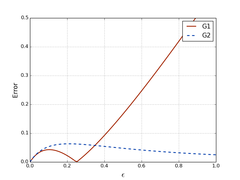
Figure 3: The figure shows explicit error $\|{\sf K}_{\epsilon}-{\sf K}\|_{2}$

IV-A Difference between (G1) and (G2)

In the asymptotic limit as $\epsilon\downarrow 0$, the two approximations (G1) and (G2) yield identical error estimates. The difference arises as $\epsilon$ becomes larger. The following Proposition provides explicit error estimates for the bias in the special linear Gaussian case.

Proposition 2

Suppose the density $\rho$ is a Gaussian $N(0,\sigma^{2}I)$ and $h(x)=H\cdot x$. Then the bias for the two approximations is given by the following closed-form formula:

$$\text{Bias for (G1):}\quad\|{\sf K}_{\epsilon}-{\sf K}\|_{2} =\epsilon\frac{\sigma^{2}-4\epsilon}{\sigma^{2}+4\epsilon}|H|,$$ (21)

$$\text{Bias for (G2):}\quad\|{\sf K}_{\epsilon}-{\sf K}\|_{2} =\epsilon\frac{\sigma^{6}}{(\sigma^{2}+4\epsilon)(\sigma^{4}+3\epsilon\sigma^{2}+4\epsilon^{2})}|H|.$$ (22)

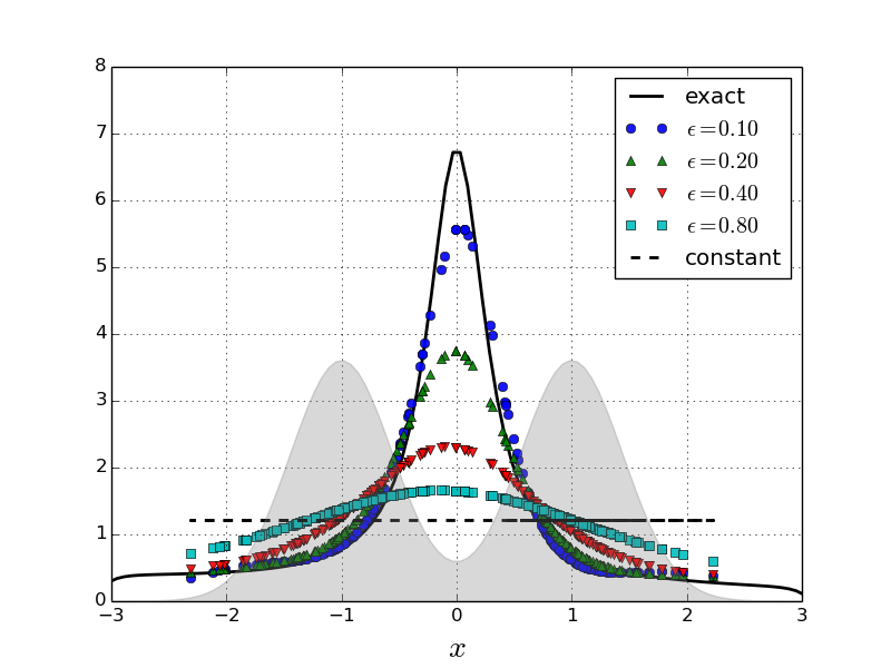
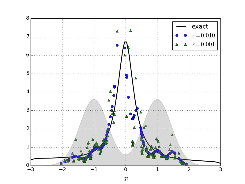
Figure 4: Numerical gain function approximation (G2) for a range of $\epsilon$. The dimension $d=1$ and the number of particles $N=200$.

Note that the bias has the same scaling, $\sim\epsilon|H|$, as $\epsilon\downarrow 0$. However as $\epsilon$ gets larger, the two approximations behave very differently. For (G1), the bias grows unbounded as $\epsilon\rightarrow\infty$. Remarkably, for (G2), the bias goes to zero as $\epsilon\rightarrow\infty$. Figure 3 depicts the bias error for a scalar example where $\sigma^{2}=1$ and $H=1$.

The following Proposition shows that the limit $\epsilon\rightarrow\infty$ is well-behaved for the (G2) approximation more generally. In fact, one recovers the constant gain approximation in that limit.

Proposition 3

Consider the gain approximation (G2) given by (15). Then,

$$\lim_{\epsilon\rightarrow\infty}\;\;{\sf K}_{\epsilon} ={\sf E}[K],$$

$$\lim_{\epsilon\rightarrow\infty}\;\;{\sf K}_{\epsilon}^{(N)} =\frac{1}{N}\sum_{i=1}^{N}(h(X^{i})-\hat{h}^{(N)})X^{i}.$$

 

V Numerics

Suppose the density $\rho$ is a mixture of two Gaussians, $\frac{1}{2}{\cal N}(-\mu,\sigma^{2}I)+\frac{1}{2}{\cal N}(+\mu,\sigma^{2}I)$, where $\mu=[1,0,\ldots,0]\in\mathbb{R}^{d}$, and $\sigma^{2}=0.2$. The observation function $h(x)=x_{1}$. In this case, the exact gain function ${\sf K}(x)=[{\sf K}_{1}(x),0,\ldots,0]$ where ${\sf K}_{1}(\cdot)$ is obtained using the explicit formula (5) as in the scalar case.

Figure 4 depicts a comparison between the exact solution and the approximate solution obtained using the kernel approximation formula (G2). The dimension $d=1$ and the number of particles $N=200$.

• The part (a) of the figure depicts the gain function for a range of (relatively large) $\epsilon$ values $\{0.1,0.2,0.4,0.8\}$ where the error is dominated by the bias. The constant gain approximation is also depicted and, consistent with Proposition 3, the (G2) approximation converges to the constant as $\epsilon$ gets larger.

• The part (b) of the figure depicts a comparison for a range of (very small) $\epsilon$ values $\{0.01,0.001\}$. At $N=200$ particles, the error in this range is dominated by the variance. This is manifested in a somewhat irregular spread of the particles for these $\epsilon$ values.

In the next study, we experimentally evaluated the error for a range of $\epsilon$ and $d$, again with a fixed $N=200$. For a single simulation, the error is defined as

$$\text{Error}:=\sqrt{\frac{1}{N}\sum_{i=1}^{N}|{\sf K}_{\epsilon}^{(N)}(X^{i})-{\sf K}(X^{i})|^{2}}.$$

Figure 5 and 5 depict the averaged error obtained from averaging over $M=100$ simulations. In each simulation, the parameters $\epsilon$ and $d$ are fixed but a different realization of $N=200$ particles is sampled from the density $\rho$.

• Figure 5 depicts the averaged error as $\epsilon$ and $d$ are varied. As $\epsilon$ becomes large, the kernel gain converges the constant gain formula. For relatively large values of $\epsilon$, the error is dominated by bias which is insensitive to the size of dimension $d$.

• Figure 5 depicts the averaged error for small values of $\epsilon$. The logarithmic scale is used to better assess the asymptotic characteristics of the error as a function of $\epsilon$ and $d$. Recall that the estimates in Theorem 2 predict that the error scales as $\epsilon^{-1-d/4}$ for the small $\epsilon$ large $N$ limit. To verify the prediction, an empirical exponent was computed by fitting a linear curve to the error data on the logarithmic scale. The empirical exponents together with the error estimates predicted by Theorem 2 are tabulated in Table I. It is observed that the empirical exponents are smaller than the predictions. The gap suggests that the error bound may not be tight. A more thorough comparison is a subject of continuing investigation.

$d$	$1$	$2$	$3$	$4$
$1+d/4$	$1.25$	$1.5$	$1.75$	$2.0$
$\alpha$	$0.83$	$1.12$	$1.36$	$1.56$

TABLE I: Comparison of empirically obtained exponents ($\alpha$) with the theoretical exponents $1+d/4$. Empirical exponents are obtained by curve fitting the data in Fig. 5.

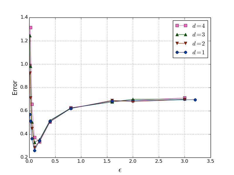
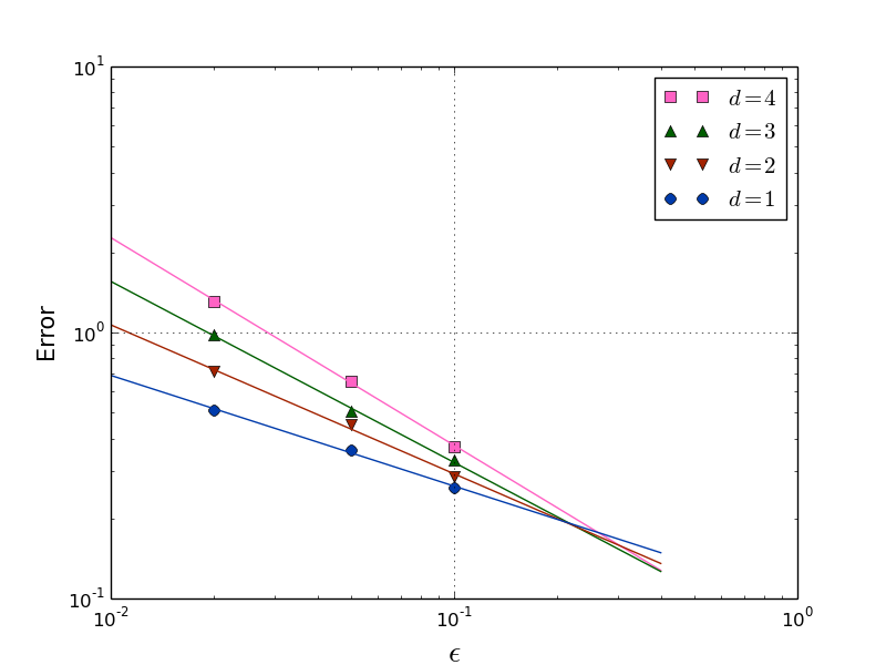
Figure 5: Averaged error over $M=100$ simulations with $N=200$ particles: (a) Linear scale over a range of $\epsilon$ and (b) Logarithmic scale for small $\epsilon$.

-A Kernel-based algorithm

This section provides additional details for the kernel-based algorithm presented in Sec. III. We begin with some definitions and then provide justification for the three main steps, fixed-point equations (8)-(10).

Definitions: The Gaussian kernel is denoted as $g_{\epsilon}(x,y):=\exp(-\frac{\|x-y\|^{2}}{4\epsilon})$. The approximating family of operators $\{{T}_{\epsilon},\epsilon\geq 0\}$ are defined as follows: For $f:\mathbb{R}^{d}\to\mathbb{R}$,

$${T}_{\epsilon}f(x):=\int_{\mathbb{R}^{d}}k_{\epsilon}(x,y)f(y)\rho(y)\,\mathrm{d}y,$$ (23)

where

$${k}_{\epsilon}:(x,y)=\frac{1}{n_{\epsilon}(x)}\frac{g_{\epsilon}(x,y)}{\sqrt{\int g_{\epsilon}(y,z)\rho(z)\,\mathrm{d}z}},$$

and $n_{\epsilon}$ is the normalization factor, chosen such that $\int{k}_{\epsilon}(x,y)\rho(y)\,\mathrm{d}y=1$. The finite-$N$ approximation of these operators, denoted as $\{{T}^{(N)}_{\epsilon}\}_{\epsilon\geq 0,N\in\mathbb{N}}$, is defined as,

$${T}^{(N)}_{\epsilon}f(x):=\frac{1}{N}\sum_{i=1}^{N}{k}_{\epsilon}^{(N)}(x,X^{i})f(X^{i}),$$ (24)

where

$${k}_{\epsilon}^{(N)}(x,y):=\frac{1}{n_{\epsilon}^{(N)}(x)}\frac{{g}_{\epsilon}(x,y)}{\sqrt{\sum_{j=1}^{N}g_{\epsilon}(y,X^{j})}},$$ (25)

and $n_{\epsilon}^{(N)}$ is chosen such that $\frac{1}{N}\sum_{i=1}^{N}{k}_{\epsilon}(x,X^{i})=1$.

Justification of the fixed-point equations (8)-(10):

(i) Definition of the semigroup $e^{\epsilon\Delta_{\rho}}$ implies:

$$e^{\epsilon\Delta_{\rho}}f=f+\int_{0}^{\epsilon}e^{s\Delta_{\rho}}\Delta_{\rho}f\,\mathrm{d}s$$

On choosing $f=\phi$ where $\Delta_{\rho}\phi=-(h-\hat{h})$ yields the exact fixed point equation (8).

(ii) The justification for approximation ${T}_{\epsilon}\approx e^{\epsilon\Delta_{\rho}}$ is the following Lemma.

Lemma 1

Consider the family of Markov operators $\{{T}_{\epsilon}\}_{\epsilon\geq 0}$. Fix a smooth function $f$. Then

$${T}_{\epsilon}f(x)=f(x)+\epsilon\Delta_{\rho}f(x)+O(\epsilon^{2}).$$ (26)

Proof:

Introduce the heat semigroup ${G}_{\epsilon}$ as,

$$G_{\epsilon}f(x):=\int_{\mathbb{R}^{d}}g_{\epsilon}(x-y)f(y)\rho(y)\,\mathrm{d}y.$$ (27)

The following are the two properties of the heat semigroup:

$$G_{0}f(x) =\rho(x)f(x),$$ (28)

$$\frac{\,\mathrm{d}}{\,\mathrm{d}\epsilon}G_{\epsilon}f(x)\big{|}_{\epsilon=0} =\Delta(\rho f)(x).$$ (29)

In terms of ${G}_{\epsilon}$, the operator ${T}_{\epsilon}$ is expressed as,

$${T}_{\epsilon}f(x)=\frac{1}{n_{\epsilon}(x)}{G}_{\epsilon}(\frac{f}{\sqrt{{G}_{\epsilon}1}})(x),$$ (30)

where $n_{\epsilon}(x)={G}_{\epsilon}(\frac{1}{\sqrt{{G}_{\epsilon}1}})(x)$. The Taylor expansion of ${T}_{\epsilon}f(x)$ yields,

$$T_{\epsilon}f(x) =T_{0}f(x)+\epsilon\frac{\,\mathrm{d}}{\,\mathrm{d}\epsilon}{T}_{\epsilon}f(x)\big{|}_{\epsilon=0}+O(\epsilon^{2}).$$

Now, the properties (28) and (29) can be used to show that $T_{0}f(x)=f(x)$ and $\frac{\,\mathrm{d}}{\,\mathrm{d}\epsilon}{T}_{\epsilon}f(x)\big{|}_{\epsilon=0}=\Delta_{\rho}f(x)$.  

(iii) The justification for the third step is Law of Large numbers. Moreover the following lemma provides a bound for the $L^{2}$ error.

Lemma 2

Consider the Markov operators ${T}_{\epsilon}$ and ${T}^{(N)}_{\epsilon}$ defined in (23) and (24). Then $\forall f\in L^{2}(\rho)$,

$${\sf E}\left[\|{T}_{\epsilon}f-{T}^{(N)}_{\epsilon}f\|_{L^{2}(\rho)}^{2}\right]\leq\frac{C}{N\epsilon^{d/2}}.$$

Proof:

The bound is proved by explicitly evaluating the error ${\sf E}\left[\|{G}_{\epsilon}f-G_{\epsilon}^{(N)}f\|_{L^{2}(\rho)}^{2}\right]$ where ${G}_{\epsilon}$ is defined in (27) and $G_{\epsilon}^{(N)}f(x):=\frac{1}{N}\sum_{i=1}^{N}g_{\epsilon}(x,X^{i})f(X^{i})$. Since $\{X^{i}\}$ are i.i.d.,

$${\sf E}\left[\|{G}_{\epsilon}f-G_{\epsilon}^{(N)}f\|_{2}\right]\leq\frac{1}{N}\int\int g_{\epsilon}^{2}(x,y)f(y)^{2}\rho(y)\rho(x)\,\mathrm{d}y\,\mathrm{d}x.$$

Subsequently, using the fact that $g_{\epsilon}^{2}(x,y)=\frac{C}{\epsilon^{d/2}}g_{2\epsilon}(x,y)$ and $\int g_{2\epsilon}(x,y)\rho(x)\,\mathrm{d}x\leq C$, one obtains,

$${\sf E}\left[\|{G}_{\epsilon}f-{G}_{\epsilon}^{(N)}f\|_{L^{2}(\rho)}^{2}\right]\leq\frac{C\|f\|^{2}_{L^{2}(\rho)}}{N\epsilon^{d/2}},$$

and the estimate follows because of (30).  

-B Sketch of the Proof of Theorem 2

Estimate for Bias: The crucial property is that ${T}_{\epsilon}$ is a bounded strictly contractive operator on $H_{0}^{1}$ with

$$\|(I-{T}_{\epsilon})^{-1}\|_{H^{1}_{0}(\rho)}=\frac{1}{\epsilon\lambda_{1}}+O(1),$$ (31)

where $\lambda_{1}$ is the spectral bound for $\Delta_{\rho}$. Since ${\phi}_{\epsilon}$ solves the fixed-point equation (9),

$${\phi}_{\epsilon}={T}_{\epsilon}{\phi}_{\epsilon}+\epsilon(h-\hat{h})+O(\epsilon^{2}).$$

Therefore,

$$\phi-{\phi}_{\epsilon} =\phi-{T}_{\epsilon}\phi+{T}_{\epsilon}(\phi-{\phi}_{\epsilon})-\epsilon(h-\hat{h})+O(\epsilon^{2})$$

$$=-\epsilon\Delta_{\rho}\phi+{T}_{\epsilon}(\phi-{\phi}_{\epsilon})-\epsilon(h-\hat{h})+O(\epsilon^{2}),$$

where we have used Lemma 26. Noting $-\Delta_{\rho}\phi=(h-\hat{h})$,

$$\phi-{\phi}_{\epsilon}={T}_{\epsilon}(\phi-{\phi}_{\epsilon})+O(\epsilon^{2}).$$

The bias estimate now follows from using the norm estimate (31).

Estimate for variance: The variance estimate follows from using Lemma  2. The key steps are to show that

$$\|{T}^{(N)}_{\epsilon}f-{T}_{\epsilon}f\|_{H^{1}_{0}(\rho)}\to 0\quad\text{a.s},$$

which follows from the LLN, and that ${T}^{(N)}_{\epsilon}$ are bounded and compact on $H^{1}_{0}(\rho)$. This allows one to conclude that $\|(I-{T}^{(N)}_{\epsilon})^{-1}\|_{H^{1}_{0}(\rho)}$ is bounded. These forms of approximation error bounds in a somewhat more general context of compact operators appears in [Chapter 7 of [6]].

-C Proof of proposition 2

For the Gaussian density ${\cal N}(0,\sigma^{2}I)$, the completion of square is used to obtain an explicit form for the operator ${T}_{\epsilon}$:

$${T}_{\epsilon}f(x)=\int\frac{1}{\sqrt{4\pi\epsilon(1-\delta_{\epsilon})}}\exp\left[-\frac{(y-(1-\delta_{\epsilon})x)^{2}}{4\epsilon(1-\delta_{\epsilon})}\right]f(y)\,\mathrm{d}y,$$

where $\delta_{\epsilon}:=\epsilon\frac{\sigma^{2}+4\epsilon}{\sigma^{4}+3\epsilon\sigma^{2}+4\epsilon^{2}}$. For the linear function $h(x)=H\cdot x$, the fixed-point equation (9) admits an explicit solution,

$$\phi_{\epsilon}=\frac{\epsilon}{\delta_{\epsilon}}H\cdot x$$

where we used the fact that ${T}_{\epsilon}x=1-\delta_{\epsilon}x$.

Since the solution $\phi_{\epsilon}$ is known in an explicit form, one can easily compute the gain function solution in an explicit form:

$$\text{(G1)}\quad{\sf K}_{\epsilon} =\frac{\epsilon}{\delta_{\epsilon}}H=\sigma^{2}H-\epsilon\frac{\sigma^{2}-4\epsilon}{\sigma^{2}+4\epsilon}H,$$

$$\text{(G2)}\quad{\sf K}_{\epsilon} =\sigma^{2}H+\frac{\epsilon\sigma^{6}}{(\sigma^{2}+4\epsilon)(\sigma^{4}+3\epsilon\sigma^{2}+4\epsilon^{2})}H.$$

The error estimates follow based on the exact Kalman gain solution ${\sf K}=\sigma^{2}H$.

-D Proof of Proposition 3

The proof relies on the fact that $\epsilon^{d/2}{g}_{\epsilon}(x,y)$ converges to a constant as $\epsilon\to\infty$. This would imply that ${k}_{\epsilon}(x,y)\to 1$ as $\epsilon\to\infty$. Therefore for a fixed function $f$,

$$\lim_{\epsilon\to\infty}{T}_{\epsilon}f(x)=\int f(x)\rho(x)\,\mathrm{d}x=:\hat{f}$$

Define the limit $T_{\infty}:=\lim_{\epsilon\to\infty}{T}_{\epsilon}$ and observe:

$$\lim_{\epsilon\to\infty}\frac{{\phi}_{\epsilon}}{\epsilon}=\lim_{\epsilon\to\infty}(I-{T}_{\epsilon})^{-1}(h-\hat{h})=(I-T_{\infty})^{-1}(h-\hat{h})=h-\hat{h}$$

where the last step uses the fact that $\hat{h}=T_{\infty}h$ and we assumed $(I-{T}_{\epsilon})^{-1}h\to(I-T_{\infty})h$. Then the gain approximation formula (15) implies:

$$\lim_{\epsilon\to\infty}{\sf K}_{\epsilon}(x) =\lim_{\epsilon\to\infty}\frac{1}{2}\left[{T}_{\epsilon}(e\frac{{\phi}_{\epsilon}}{\epsilon})-{T}_{\epsilon}(e){T}_{\epsilon}(\frac{{\phi}_{\epsilon}}{\epsilon})\right]$$

$$+\lim_{\epsilon\to\infty}\frac{1}{2}\left[{T}_{\epsilon}(eh)-{T}_{\epsilon}(e){T}_{\epsilon}(h)\right]$$

$$=\int x(h(x)-\hat{h})\rho(x)\,\mathrm{d}x$$

The argument for the finite-$N$ case is identical and omitted on account of space.

References

- [1] D. Bakry, I. Gentil, and M. Ledoux. Analysis and geometry of Markov diffusion operators, volume 348. Springer Science & Business Media, 2013.
- [2] K Berntorp. Feedback particle filter: Application and evaluation. In 18th Int. Conf. Information Fusion, Washington, DC, 2015.
- [3] K. Berntorp and P. Grover. Data-driven gain computation in the feedback particle filter. In 2016 American Control Conference (ACC), pages 2711–2716. IEEE, 2016.
- [4] R. R. Coifman and S. Lafon. Diffusion maps. Applied and computational harmonic analysis, 21(1):5–30, 2006.
- [5] M. Hein, J. Audibert, and U. Luxburg. Graph laplacians and their convergence on random neighborhood graphs. Journal of Machine Learning Research, 8(Jun):1325–1368, 2007.
- [6] V. Hutson, J. Pym, and M. Cloud. Applications of functional analysis and operator theory, volume 200. Elsevier, 2005.
- [7] R. S. Laugesen, P. G. Mehta, S. P. Meyn, and M. Raginsky. Poisson’s equation in nonlinear filtering. SIAM Journal on Control and Optimization, 53(1):501–525, 2015.
- [8] Y. Matsuura, R. Ohata, K. Nakakuki, and booktitle=AIAA Guidance, Navigation, and Control Conference pages=1620 year=2016 Hirokawa, R. Suboptimal gain functions of feedback particle filter derived from continuation method.
- [9] A. Radhakrishnan, A. Devraj, and S. Meyn. Learning techniques for feedback particle filter design. In Conference on Decision and COntrol (CDC), 2016, pages 648–653. IEEE, 2014.
- [10] P. M. Stano, A. K. Tilton, and R. Babuška. Estimation of the soil-dependent time-varying parameters of the hopper sedimentation model: The FPF versus the BPF. Control Engineering Practice, 24:67–78, 2014.
- [11] A. Taghvaei and P. G. Mehta. Gain function approximation in the feedback particle filter. (To appear) in the Conference on Decision and Control (CDC), 2016, available online at arXiv:1603.05496.
- [12] A. K Tilton, S. Ghiotto, and P. G Mehta. A comparative study of nonlinear filtering techniques. In Information Fusion (FUSION), 2013 16th International Conference on, pages 1827–1834, 2013.
- [13] T. Yang, R. S. Laugesen, P. G. Mehta, and S. P. Meyn. Multivariable feedback particle filter. Automatica, 71:10–23, 2016.
- [14] T. Yang, P. G. Mehta, and S. P. Meyn. Feedback particle filter. IEEE Trans. Automatic Control, 58(10):2465–2480, October 2013.