Importance sampling-based approximate optimal planning and control

Abstract

In this paper, we propose a sampling-based planning and optimal control method of nonlinear systems under non-differentiable constraints. Motivated by developing scalable planning algorithms, we consider the optimal motion plan to be a feedback controller that can be approximated by a weighted sum of given bases. Given this approximate optimal control formulation, our main contribution is to introduce importance sampling, specifically, model-reference adaptive search algorithm, to iteratively compute the optimal weight parameters, i.e., the weights corresponding to the optimal policy function approximation given chosen bases. The key idea is to perform the search by iteratively estimating a parametrized distribution which converges to a Dirac’s Delta that infinitely peaks on the global optimal weights. Then, using this direct policy search, we incorporated trajectory-based verification to ensure that, for a class of nonlinear systems, the obtained policy is not only optimal but robust to bounded disturbances. The correctness and efficiency of the methods are demonstrated through numerical experiments including linear systems with a nonlinear cost function and motion planning for a Dubins car.

0.1 Introduction

This paper presents an importance sampling based approximate optimal planning and control algorithm. Optimal motion planning in deterministic and continuous systems is computationally NP-complete [1] except for linear time invariant systems. For nonlinear systems, there is a vast literature on approximate solutions and algorithms. In optimal planning, the common approximation scheme is discretization-based. By discretizing the state and input spaces, optimal planning is performed by solving the shortest path problem in the discrete transition systems obtained from abstracting the continuous dynamics, using heuristic-based search or dynamic programming. Comparing to discretization-based methods, sampling-based graph search, includes Probabilistic RoadMap (PRM) [2], RRT [3], RRT* [4], are more applicable for high-dimensional systems. While RRT has no guarantee on the optimality of the path [4], RRT* compute an optimal path asymptotically provided the cost functional is Lipschitz continuous. However, such Lipschitz conditions may not be satisfied for some cost functions under specific performance consideration.

The key idea in the proposed sampling-based planning method builds on a unification of importance sampling and approximate optimal control [5, 6]. In approximate optimal control, the objective is to approximate both the value function, i.e., optimal cost-to-go, and the optimal feedback policy function by weighted sums of known basis functions. As a consequence, the search space is changed from infinite trajectory space or policy space to a continuous space of weight vectors, given that each weight vector corresponds to a unique feedback controller.

Instead of solving the approximate optimal control through training actor and critic neural networks (NNs) using trajectory data [7, 8], we propose a sampling-based method for sampling the weight vectors for a policy function approximation and searching for the optimal one. This method employs Model Reference Adaptive Search (MRAS) [9], a probabilistic complete global optimization algorithm, for searching the optimal weight vector that parametrizes the approximate optimal feedback policy. The fundamental idea is to treat the weight vector as a random variable over a parameterized distribution and the optimal weight vector corresponds to a Dirac’s Delta function which is the target distribution. The MRAS algorithm iteratively estimates the parameter that possesses the minimum Kullback-Leibler divergence with respect to an intermediate reference model, which assigns a higher probability mass on a set of weights of controllers with improved performance over the previous iteration. At the meantime, a set of sampled weight vectors are generated using the parameterized distribution and the performance of their corresponding policies are evaluated via simulation-based policy evaluation. Under mild conditions, the parameterized distribution converges, with probability one, to the target distribution that concentrates on the optimal weight vector with respect to given basis functions.

MRAS resembles another adaptive search algorithm called cross-entropy(CE) method and provides faster and stronger convergence guarantee for being less sensitive to input parameters [9, 10]. Previously, CE algorithm has been introduced for motion planning [11, 12] based on sampling in the trajectory space. The center idea is to construct a probability distribution over the set of feasible paths and to perform the search for an optimal trajectory using CE. The parameters to be estimated is either a sequence of motion primitives or a set of via-points for interpolation-based trajectory planning. Differ to these methods, ours is the first to integrate importance sampling to estimate parameterization of the optimal policy function approximation for continuous nonlinear systems. Since the algorithm performs direct policy search, we are able to enforce robustness and stability conditions to ensure the computed policy is both robust and approximate optimal, provided these conditions can be evaluated efficiently.

To conclude, the contributions of this paper are the following: First, we introduce a planning algorithm by a novel integration of model reference adaptive search and approximate optimal control. Second, based on contraction theory, we introduce a modification to the planning method to directly generate stabilizing and robust feedback controllers in the presence of bounded disturbances. Last but not the least, through illustrative examples, we demonstrate the effectiveness and efficiency of the proposed methods and share our view on interesting future research along this direction.

0.2 Problem formulation

Notation: The inner product between two vectors $w,v\in\mathbf{R}^{n}$ is denoted $w^{\intercal}v$ or $\langle w,v\rangle$. Given a positive semi-definite matrix $P$, the $P$-norm of a vector is denoted $\lVert x\rVert_{P}=\sqrt{x^{\intercal}Px}$. We denote $\lVert x\rVert$ for $P$ being the identity matrix. $I_{\{E\}}$ is the indicator function, i.e., $I_{E}=1$ if event $E$ holds, otherwise $0$. For a real $\alpha\in\mathbb{R}$, $\lceil\alpha\rceil$ is the smallest integer that is greater than $\alpha$.

0.2.1 System model

We consider continuous-time nonlinear systems of the form

$$\begin{split}\Sigma:\quad&\dot{x}(t)=f(x(t),u(t)),\\ &x(t)\in X,u(t)\in U.\end{split}$$ (1)

where $x\in X$ is the state, $u\in U$ is the control input, $x_{0}\in X$ is the initial state, and $f(x,u)$ is a vector field. We assume that $X$ and $U$ are compact. A feedback controller $u:X\rightarrow U$ takes the current state and outputs a control input.

The objective is to find a feedback controller $u^{\ast}$ that minimizes a finite-horizon cost function for a nonlinear system

$$\begin{split}\min_{u}J(x_{0},u)&=\int_{0}^{T}\ell(x(t),u(t))dt+g(x(T),u(T))\\ \mbox{subject to: }&\dot{x}(t)=f(x(t),u(t)),\\ &x(t)\in X,\;u(t)\in U,\;x(0)=x_{0}.\end{split}$$ (2)

where $T$ is the stopping time, $\ell:X\times U\rightarrow\mathbb{R}^{+}$ defines the running cost when the state trajectory traverses through $x$ and the control input $u$ is applied and $g:X\rightarrow\mathbb{R}^{+}$ defines the terminal cost. As an example, a running cost function can be a quadratic cost $\ell(x,u)=\lVert x\rVert_{R}+\lVert u\rVert_{Q}$ for some positive semi-definite matrices $Q$ and $R$, and a terminal cost can be $g(x,u)=\lVert x-x_{f}\rVert_{R}$ where $x_{f}$ is a goal state.

We denote the set of feedback policies to be $\Pi$. For infinite horizon optimal control, the optimal policy is independent of time and a feedback controller suffices to be a minimizing argument of (2) (see Ref. [13]). For finite-horizon optimal control, the optimal policy is time-dependent. However, for simplicity, in this paper, we only consider time-invariant feedback policies and assume the time horizon $T$ is of sufficient length to ignore the time constraints.

0.2.2 Preliminary: Model reference adaptive search

MRAS algorithm, introduced in [9], aims to solve the following problem:

$$z^{\ast}\in\arg\max_{z\in Z}H(z),\quad z\in\mathbf{R}^{n}$$

where $Z$ is the solution space and $H:\mathbf{R}^{n}\rightarrow\mathbf{R}$ is a deterministic function that is bounded from below. It is assumed that the optimization problem has a unique solution, i.e., $z^{\ast}\in Z$ and for all $z\neq z^{\ast}$, $H(z)<H(z^{\ast})$.

The following regularity conditions need to be met for the applicability of MRAS.

Assumption 1.

For any given constant $\xi<H(z^{\ast})$, the set $\{z\mid H(z)\geq\xi\}\cap Z$ has a strictly positive Lebesgue or discrete measure.

This condition ensures that any neighborhood of the optimal solution $z^{\ast}$ will have a positive probability to be sampled.

Assumption 2.

For any constant $\delta>0$, $\sup_{z\in A_{\delta}}H(z)<H(z^{\ast})$, where $A_{\delta}:=\{z\mid\lVert z-z^{\ast}\rVert\geq\delta\}\cap X$, and we define the supremum over the empty set to be $-\infty$.

• Selecte a sequence of reference distributions $\{g_{k}(\cdot)\}$ with desired convergence properties. Specifically, the sequence $\{g_{k}(\cdot)\}$ will converge to a distribution that concentrates only on the optimal solution.

• Selecte a parametrized family of distribution $f(\cdot,\theta)$ over $X$ with parameter $\theta\in\Theta$.

• Optimize the parameters $\{\theta_{k}\}$ iteratively by minimizing the following KL distance between $f(\cdot,\theta_{k})$ and $g_{k}(\cdot)$.

  $$d(g_{k},f(\cdot,\theta)):=\int_{Z}\ln\frac{g_{k}(z)}{f(z,\theta)}g_{k}(z)\nu(dz).$$

  where $\nu(\cdot)$ is the Lebesgue measure defined over $Z$. The sample distributions $\{f(\cdot,\theta_{k})\}$ can be viewed as compact approximations of the reference distributions and will converge to an approximate optimal solution as $\{g_{k}(\cdot)\}$ converges provided certain properties of $\{g_{k}(\cdot)\}$ is retained in $f(\cdot,\theta_{k})$.

Note that the reference distribution $\{g_{k}(\cdot)\}$ is unknown beforehand as the optimal solution is unknown. Thus, the MRAS algorithm employs the estimation of distribution algorithms [14] to estimate a reference distribution that guides the search. To make the paper self-contained, we will cover details of MRAS in the development of the planning algorithm.

0.3 Approximate optimal motion planning using MRAS

In this section, we present an algorithm that uses MRAS in a distinguished way for approximate optimal feedback motion planning.

0.3.1 Policy function approximation

The policy function approximation $\bar{u}:X\rightarrow U$ is a weighted sum of basis functions,

$$\bar{u}(x)=\sum_{i=1}^{N}w_{i}\phi_{i}(x)$$

where $\phi_{i}:X\rightarrow\mathbf{R},i=1,\ldots,N$ are basis functions, and the coefficients $w_{i}$ are the weight parameters, $i=1,\ldots,N$. An example of basis function can be polynomial basis $\phi=[1,x,x^{2},x^{3},\ldots,x^{N}]$ for one-dimensional system. A commonly used class of basis functions is Radial basis function (RBF). It can be constructed by determining a set of centers $c_{i},\ldots,c_{N}\in X$, and then constructing RBF basis functions $\phi_{i}=\exp(-\frac{\lVert x-c_{i}\rVert^{2}}{2\sigma^{2}})$, for each center $c_{i}$, where $\sigma$ is a pre-defined parameter.

In vector form, a policy function approximation is represented by $\bar{u}=\langle w,\phi\rangle$ where vector $\phi=\left[\phi_{1},\ldots\phi_{N}\right]^{\intercal}$ and $w=[w_{1},\ldots,w_{N}]^{\intercal}$. We let the domain of weight vector be $W$ and denote it by $\Pi_{\phi}=\{\langle w,\phi\rangle\mid w\in W,\langle w,\phi\rangle\in\Pi\}$ the set of all policies that can be generated by linear combinations of pre-defined basis functions. In the following context, unless specifically mentioned, the vector of basis functions is $\phi$.

Clearly, for any weight vector $w$, $J(x_{0},\langle w,\phi\rangle)\geq\min_{u\in\Pi}J(x_{0},u)$. Thus, we aim to solve $\min_{w}J(x_{0},\langle w,\phi\rangle)$ so as to minimize the error in the optimal cost introduced by policy function approximation.

Definition 1 (Approximate optimal feedback policy).

Given a basis vector $\phi$, a weight vector $w^{\ast}$ with respect to $\phi$ is optimal if and only if $\langle w^{\ast},\phi\rangle\in\Pi_{\phi}$ and for all $w\in W$ such that $\langle w,\phi\rangle\in\Pi_{\phi}$,

$$J(x_{0},\langle w^{\ast},\phi\rangle)\leq J(x_{0},\langle w,\phi\rangle).$$

The approximate optimal feedback policy is $\bar{u}^{\ast}=\langle w^{\ast},\phi\rangle$.

By requiring $J(x_{0},\langle w^{\ast},\phi\rangle)\leq J(x_{0},\langle w,\phi\rangle)$, it can be shown that the optimal weight vector $w^{\ast}$ minimizes the difference between the optimal cost achievable with policies in $\Pi_{\phi}$ and the cost under the global optimal policy.

For clarity in notation, we denote $J(x_{0},\langle w,\phi\rangle)$ by $J(x_{0};w)$ as $\phi$ is a fixed basis vector throughout the development of the proposed method.

Clearly, if the actual optimal policy $u^{\ast}$ can be represented by a linear combination of selected basis functions, then we obtain the optimal policy by computing the optimal weight vector, i.e., $u^{\ast}=\langle w^{\ast},\phi\rangle$.

Remark:

Here, we assume a feedback policy can be represented by $\langle w,\phi\rangle$ for some weight vector $w\in W$. In cases when the basis functions are continuous, a feedback policy must be a continuous function of the state. However, this requirement is hard to satisfy for many physical systems due to, for example, input saturation. In cases when a feasible controller is discontinuous, we can still use a continuous function to approximate, and then project the continuous function to the set $\Pi$ of applicable controllers.

Using function approximation, we aim to solve the optimal feedback planning problem in (2) approximately by finding the optimal weight vector with respect to a pre-defined basis vector. The main algorithm is presented next.

0.3.2 Integrating MRAS in approximate optimal planning

In this section, we present an adaptive search-based algorithm to compute the approximate optimal feedback policy. The algorithm is “near” anytime, meaning that it returns a feasible solution after a small number of samples. If more time is permitted, it will quickly converge to the globally optimal solution that corresponds to the approximate optimal feedback policy. The algorithm is probabilistic complete under regularity conditions of MRAS.

We start by viewing the weight vector as a random variable $\mathbf{w}$ governed by a multivariate Gaussian distribution with a compact support $W$. The distribution is parameterized by parameter $\theta=(\mu,\Sigma)$, where $\mu$ is a $N$-dimensional mean vector and $\Sigma$ is the $N$ by $N$ covariance matrix. Recall $N$ is the number of basis functions.

The optimal weight vector $w^{\ast}$ can be represented as a target distribution $p_{\mathsf{goal}}$ as a Dirac’s Delta, i.e., $p_{\mathsf{goal}}(w^{\ast})=\infty$ and $p_{\mathsf{goal}}(w)=0$ for $w\neq w^{\ast}$. Dirac’s Delta is a special case of multivariate Gaussian distribution with zero in the limit case of vanishing covariance. Thus, it is ensured that the target distribution can be arbitrarily closely approximated by multivariate Gaussian distribution by a realization of parameter $\theta$.

Recall that the probability density of a multivariate Gaussian distribution is defined by

$$p(w;\theta)=\frac{1}{\sqrt{(2\pi)^{N}\lvert\Sigma\rvert}}\exp(-\frac{1}{2}(x-\mu)^{\intercal}\Sigma^{-1}(x-\mu)),$$

$$\theta=(\mu,\Sigma),\forall w\in W,$$

where $N$ is the dimension of weight vector $w\in W$ and $\lvert\Sigma\rvert$ is the determinant of $\Sigma$.

Now, we are ready to represent the main algorithm, called Sampling-based Approximate-Optimal Planning (SAOP), which includes the following steps.

1. Initialization: The initial distribution is selected to be $p(\cdot,\theta_{0})$, for $\theta_{0}=(\mu_{0},\Sigma_{0})\in\Theta$ which can generate a set of sample to achieve a good coverage of the sample space $W$. For example, $\mu_{0}=\mathbf{0}\in\mathbf{R}^{N}$ and $\Sigma_{0}=\mathbf{I}\in\mathbf{R}^{N}$ which is an identity matrix. The following parameters are used in this algorithm: $\rho\in(0,1]$ for specifying the quantile, the improvement parameter $\varepsilon\in\mathbf{R}^{+}$, a sample increment percentage $\alpha$, an initial sample size $N_{1}$, a smoothing coefficient $\lambda\in(0,1]$. Let $k=1$.

2. Sampling-based policy evaluation: At each iteration $k$, generate a set of $N_{k}$ samples $W_{k}\subseteq W$ from the current distribution $p(\cdot,\theta_{k})$. For each $w\in W_{k}$, using simulation we evaluate the cost $J(x_{0};w)$ from the initial state $x_{0}$ and the feedback policy $u(x)=\langle w,\phi(x)\rangle$ with system model in (1). The cost $J(x_{0};w)$ is determined because the system is deterministic and has a unique solution.

3. Policy improvement with Elite samples: Next, the set $\{J(x_{0};w)\mid w\in W_{k}\}$ is ordered from largest (worst) to smallest (best) among given samples:

   $$J_{k,(0)}\geq\ldots\geq J_{k,(N_{k})}$$

   We denote $\kappa$ to be the estimated $(1-\rho)$-quantile of cost $J(\cdot;w)$, i.e., $\kappa=J_{k,\lceil(1-\rho)N_{k}\rceil}$.

   The following cases are distinguished.

   • If $k=1$, we introduce a threshold $\gamma=\kappa$.

   • If $k\neq 1$, the following cases are further distinguished:

     • $\kappa\leq\gamma-\varepsilon$, i.e., the estimated $(1-\rho)$-quantile of cost has been reduced by the amount of $\varepsilon$ from the last iteration, then let $\gamma=\kappa$. Let $N_{k+1}=N_{k}$ and continue to step 4).

     • Otherwise $\kappa>\gamma-\varepsilon$, we find the largest $\rho^{\prime}$, if it exists, such that the estimated $(1-\rho^{\prime})$-quantile of cost $\kappa^{\prime}=J_{k,\lceil(1-\rho^{\prime})N_{k}\rceil}$ satisfies $\kappa^{\prime}\leq\gamma-\varepsilon$. Then let $\gamma=\kappa^{\prime}$ and also let $\rho=\rho^{\prime}$. Continue to step 4). However, if no such $\rho^{\prime}$ exists, then there is no update in the threshold $\gamma$ but the sample size is increased to $N_{k+1}=\lceil(1+\alpha)N_{k}\rceil$. Let $\theta_{k+1}=\theta_{k}$, $k=k+1$, and continue to step 2).

   • Parameter(Policy) update: We update parameters $\theta_{k+1}$ for iteration $k+1$. First, we define a set $E=\{w\mid J(x_{0};w)\leq\gamma,w\in W_{k},j=1,\ldots,k\}$ of elite samples. Note that the parameter update in $\theta$ is to ensure a higher probability for elite samples. To achieve that, for each elite sample $w\in E$, we associated a weight such that a higher weight is associated with a weight vector with a lower cost and a lower probability in the current distribution. The next parameter $\theta_{k+1}$ is selected to maximize the weighted sum of probabilities of elite samples. To this end, we update the parameter as follows.

     $$\theta_{k+1}^{\ast}\\ =\arg\max_{\theta\in\Theta}\mathbb{E}_{\theta_{k}}\left[\frac{S(J(x_{0},w))^{k}}{p(w,\theta_{k})}I_{J(x_{0},w)\leq\gamma}\ln p(w,\theta)\right]$$

     where $\mathbb{E}_{\theta}(\nu)$ is the expected value of a random variable $\nu$ given distribution $p(\cdot,\theta)$, $S:\mathbf{R}\rightarrow\mathbf{R}^{+}$ is a strictly decreasing and positive function . $S(J(x_{0};w))^{k}/p(w,\theta_{k})$ is the weight for parameter $w$.

Assumption 3.

The optimal parameter $\theta^{\ast}$ is the interior point of $\Theta$ for all $k$.

Lemma 1 (based on Theorem 1 [9]).

Assuming  1,2, and 3 and the compactness of $W$, with probability one,

$$\lim_{k\rightarrow\infty}\mu_{k}=w^{\ast},\text{ and }\lim_{k\rightarrow\infty}\Sigma_{k}=0_{N\times N}.$$

where $w^{\ast}$ is the optimal weight vector and $0_{N\times N}$ is an $N$-by-$N$ zero matrix.

Note that since $\Sigma_{k}$ converges in the limit a zero matrix, the stopping criterion is justified.

Building on the convergence result of MRAS, the proposed sampling-based planner ensures a convergence to a Dirac Delta function concentrating on the optimum. In practice, the parameter update is performed using the expectation—maximization (EM) algorithm.

EM-based parameter update/policy improvement Since our choice of probability distribution is the multivariate Gaussian, the parameter $\theta^{\ast}_{k+1}=(\mathbf{\mu},\Sigma)$ is computed as follows

$$\mathbf{\mu}=\frac{\mathbb{E}_{\theta_{k}}[S(J(x_{0},w))^{k}/p(w,\theta_{k})]I_{w\in E}w}{\mathbb{E}_{\theta_{k}}[S(J(x_{0},w))^{k}/p(w,\theta_{k})]I_{w\in E}}\\ \approx\frac{\sum_{w\in W_{k}}[S(J(x_{0},w))^{k}/p(w,\theta_{k})]I_{w\in E}w}{\sum_{w\in W_{k}}[S(J(x_{0},w))^{k}/p(w,\theta_{k})]I_{w\in E}},$$ (3)

and

$$\Sigma=\frac{\mathbb{E}_{\theta_{k}}[S(J(x_{0},w))^{k}/p(w,\theta_{k})]I_{w\in E}(w-\mathbf{\mu})(w-\mathbf{\mu})^{\intercal}}{\mathbb{E}_{\theta_{k}}[S(J(x_{0},w))^{k}/p(w,\theta_{k})]I_{w\in E}}\\ \approx\frac{\sum_{w\in W_{k}}[S(J(x_{0},w))^{k}/p(w,\theta_{k})]I_{w\in E}(w-\mathbf{\mu})(w-\mathbf{\mu})^{\intercal}}{\sum_{w\in W_{k}}[S(J(x_{0},w))^{k}/p(w,\theta_{k})]I_{w\in E}},$$ (4)

where we approximate $\mathbb{E}_{\theta_{k}}(h(\mathbf{w}))$ with its estimate $\frac{1}{N_{k}}\sum_{w\in W_{k}}h(w)$ for $\mathbf{w}\sim p(\cdot,\theta_{k})$ and the fraction $\frac{1}{N_{k}}$ was canceled as the term is shared by the numerator and the denominator.

Smoothing: Due to limited sample size, a greedy maximization for parameter update can be premature if too few samples are used. To ensure the convergence to the global optimal solution, a smoothing update is needed. To this end, we select the parameter for the next iteration to be

$$\theta_{k+1}\leftarrow\lambda\theta_{k}+(1-\lambda)\theta^{\ast}_{k+1}.$$

where $\lambda\in[0,1)$ is the smoothing parameter.

Let $k=k+1$. We check if the iteration can be terminated based on a given stopping criterion. If the stopping criterion is met, then we output the latest $\theta_{k}$. Otherwise, we continue to update of $\theta$ by moving to step 2).

Stopping criterion Given the probability distribution will converge to a degenerated one that concentrates on the optimal weight vector. We stop the iteration if the covariance matrix $\Sigma_{k}$ becomes near-singular given the convergence condition in Lemma 1.

To conclude, the proposed algorithm using MRAS is probabilistic complete and converges to the global optimal solution. If the assumptions are not met, the algorithm converges to a local optimum.

0.3.3 Robust control using trajectory verification in sampling

Being able to directly search within continuous control policy space, one major advantage is that one can enforce stability condition such that the search is restricted to stable and robust policy space. In this subsection, we consider contraction theory to compute conditions that need to be satisfied by weight vectors to ensure stability and robustness under bounded disturbances.

Definition 2.

[15] Given the system equation for the closed-loop system $\dot{x}=f(x,t)$, a region of the state space is called a contraction region if the Jacobian $\frac{\partial f}{\partial x}$ is uniformly negative definite in that region, that is,

$$\exists\beta>0,\forall x,\forall t>0,\frac{1}{2}\left(\frac{\partial f}{\partial x}M+\dot{M}+M\frac{\partial f}{\partial x}^{\intercal}\right)\preceq-\beta M.$$

where $M(t)$ is a positive definite matrix for all $t\geq 0$.

Theorem 1.

[15] Given the system model $\dot{x}=f(x,t)$, any trajectory, which starts in a ball of constant radius with respect to the matrix $M$, centered about a given trajectory and contained at all times in a contraction region with respect to the matrix $M$, remains in that ball and converges exponentially to this trajectory. Furthermore, global exponential convergence to the given trajectory is guaranteed if the whole state space is a contraction region.

Theorem 1 provides a necessary and sufficient condition for exponential convergence of an autonomous system. Under bounded disturbances, the key idea is to incorporate a contraction analysis in the planning algorithm such that it searches for a weight vector $w$ that is not only optimal in the nominal system but also ensures that the closed-loop actual system under the controller $u=w^{\intercal}\phi$ has contraction dynamics within a tube around the nominal trajectory. Using a similar proof in [16], we can show that for systems with contracting dynamics, the actual trajectory under bounded disturbances will be ultimately uniformly bounded along the nominal trajectory.

Lemma 2.

Consider a closed-loop system $\dot{x}=f(x)+\omega(t)$ where $\omega(t)$ is a disturbance with $\max_{t}\lVert\omega(t)\rVert\leq\rho_{\max}$, let a state trajectory $x(t)$ be in the contraction region $X_{\ell}$ at all time $t\geq t_{0}$, then for any time $t\geq t_{0}$, the deviation between $x(t)$ and the nominal trajectory $\bar{x}(t)$, whose dynamic model is given by $\dot{\bar{x}}=f(\bar{x})$, satisfies

$$\lVert x(t)-\bar{x}(t)\rVert_{M}^{2}\leq\frac{2\ell\rho_{\max}}{\beta}(1-e^{\beta t}))$$

In other words, the error is uniformly ultimately bounded with the ultimate bound $\frac{2\ell\rho_{\max}}{\beta}$.

Proof.

Let’s pick the Lyapunov function

$$V=(x-\bar{x})^{T}M(x-\bar{x}),$$

whose time derivative is

$$\dot{V} =(x-\bar{x})^{T}M(f(x)+\omega-f(\bar{x}))$$

$$+(f(x)+\omega-f(\bar{x}))^{T}M(x-\bar{x})$$

$$=(x-\bar{x})^{T}M(f(x)-f(\bar{x}))+2(x-\bar{x})^{T}M\omega$$

$$(M\mbox{ is symmetric})$$

$$=(x-\bar{x})^{T}(\frac{\partial f}{\partial x}^{T}\mid_{\tilde{x}}M+M\frac{\partial f}{\partial x}\mid_{\tilde{x}})(x-\bar{x})$$

$$+2(x-\bar{x})^{T}M\omega,$$

where the following property is used: $f(x)-f(\bar{x})=\frac{\partial f}{\partial x}^{T}\mid_{\tilde{x}}(x-\bar{x})$ for some $\tilde{x}\in[\bar{x},x]$ if $\bar{x}\preccurlyeq x$ or $\tilde{x}\in[x,\bar{x}]$ otherwise.

Since the trajectories stays within the contraction region, the following condition holds $\frac{\partial f}{\partial x}^{T}\mid_{\tilde{x}}M+M\frac{\partial f}{\partial x}\mid_{\tilde{x}}\leq-2\beta M$, and we have

$$\dot{V}\leq-(x-\bar{x})^{T}\beta M(x-\bar{x})+2(x-\bar{x})^{T}M\omega.$$

Meanwhile, $\lVert x(t)-\bar{x}(t)\rVert_{M}\leq\ell$ as the trajectory $x(t)$ stays within the region of contraction, and also

$$M(x-\bar{x})\leq\sqrt{(x-\bar{x})^{T}MM(x-\bar{x})}=\sqrt{\lVert x-\bar{x}\rVert_{M}}$$

we conclude that as $\omega\leq\rho_{\max}$,

$$\dot{V}\leq-(x-\bar{x})^{T}(\beta M)(x-\bar{x})+2\omega\sqrt{\lVert x-\bar{x}\rVert_{M}}\\ \leq-(x-\bar{x})^{T}(\beta M)(x-\bar{x})+2\rho_{\max}\ell,$$

Since $\dot{V}\leq-\beta V+2\rho_{\max}\ell$ and under the condition that $x(0)=\bar{x}(0)$, we obtain $V(t)\leq\frac{2\ell}{\beta}\rho_{\max}(1-e^{-\beta t})$, and therefore

$$\lVert x-\bar{x}\rVert_{M}^{2}=\frac{2\ell}{\beta}\rho_{\max}(1-e^{-\beta t})$$

∎

Thus, to search for the optimal and robust policies, we modify the algorithm by introducing the following step.

Contraction verification step: Suppose the closed-loop system is subject to bounded disturbances, the objective is to ensure the trajectory is contracting within the time-varying tube $\{x\mid\lVert x-\bar{x}\rVert\leq\ell\}$, for all $t$, where $\bar{x}$ is the nominal state trajectory. The following condition translates the contraction condition into verifiable condition for a closed-loop system: Choose positive constants $\beta$, a positive definite symmetric and constant matrix $M=[m_{ij}]_{i=1,\ldots,n,j=1,\ldots,n}$, and verify whether, at each time step along the nominal trajectory $\bar{x}(t)$ in the closed-loop system under control $u(t)=w^{\intercal}\phi(x(t))$, the following condition holds.

$$\begin{split}\max_{x:\lVert x-\bar{x}\rVert_{M}\leq\ell}g_{ij}(x)\leq-\beta m_{ij},\quad\forall i=1,\ldots,n,\;\forall j=1,\ldots,n\end{split}$$ (5)

where $g_{ij}$ is the $(i,j)$th component in the matrix $\frac{\partial f}{\partial x}^{\intercal}M+M\frac{\partial f}{\partial x}$. We verify this condition numerically at discrete time steps instead of continous time. Further, if the function $g_{ij}(x)$ is semi-continuous, according to the Extreme Value Theorem, this condition can be verified by evaluating $g_{ij}(x)$ at all critical points where $\frac{dg_{ij}(x)}{dx}=0$ and the boundary of the set $\{x\mid\lVert x-\bar{x}\rVert_{M}\leq\ell\}$.

The modification to the planning algorithm is made in Step 3), if a controller $u=\langle w,\phi\rangle$ of elite sample $w$ does not meet the condition, then $w$ is rejected from the set of elite samples. Alternatively, one can do so implicitly by associating $w$ with a very large cost. However, since the condition is sufficient but not necessary as we have the matrix $M$, constant $\beta$ and $\ell$ pre-fixed and $M$ is chosen to be a constant matrix, the obtained robust controller may not necessary be optimal among all robust controllers in $\Pi_{\phi}$. A topic for future work is to extend joint planning and control policies with respect to adaptive bound $\beta$, $\ell$, and a uniformly positive definite and time-varying matrix $M(x,t)$.

0.4 Examples

In this section, we use two examples to illustrate the correctness and efficiency of the proposed method. The simulation experiments are implemented in MATLAB on a desktop with Intel Xeon E5 CPU and 16 GB of RAM.

0.4.1 Feedback gain search for linear systems

To illustrate the correctness and sampling efficiency in the planning algorithm, we consider an optimal control of linear time invariant (LTI) systems with non-quadratic cost. For this class of optimal control problems, since there is no admissible heuristic, one cannot use any planning algorithm facilitated by the usage of a heuristic function. Moreover, the optimal controller is nonlinear given the non-quadratic cost.

Consider a LTI system

$$\dot{x}=Ax+Bu$$

where $A=\begin{bmatrix}-1&1\\ 0&0\end{bmatrix}$ and $B=\begin{bmatrix}0\\ 1\end{bmatrix}$ with $x\in X=\mathbf{R}^{2}$ and $u\in\mathbf{R}^{1}$. The initial state is $x_{0}=[5,5]$.

The cost functional is $J(x_{0},u)=\int_{0}^{T}(\lVert x\rVert^{2}+\lVert u\rVert^{2}+0.5\lVert x\rVert^{4}+0.8\lVert x\rVert^{6})dt+\lVert x(T)\rVert^{2}.$

For a non-quadratic cost functional, the optimal controller is no longer linear and cannot be computed by LQR unless the running cost can be written in the sum-of-square form. Thus, we consider an approximate feedback controller with basis vector $\phi=[x_{1},x_{2},x_{1}^{2},x_{2}^{2},x_{1}^{3},x_{2}^{3}]^{\intercal}$. Suppose the magnitude of external disturbance is bounded by $\rho_{\max}=0.5$.

The following parameters are used in stability verification: $\beta=2$, at any time $t$, for all $x$ such that $\lVert x(t)-\bar{x}(t)\rVert\leq\ell$, the controller ensures $\lVert x(t)-\bar{x}(t)\rVert\leq\frac{2\ell\rho_{\max}}{\beta}(1-e^{\beta t})$ because $2\frac{\ell\rho_{\max}}{\beta}=0.5\ell\leq\ell$. With this choice for stability analysis, the constraint

$$\frac{\partial f}{\partial x}+\frac{\partial f}{\partial x}^{\intercal} =\begin{bmatrix}-2&3w(5)x_{1}^{2}+2w(3)x_{1}+w(1)+1\\ \mbox{Sym.}&6w(6)x_{2}^{2}+4w(4)x_{2}+2w(2)\end{bmatrix}$$

$$\leq\begin{bmatrix}-2&0\\ 0&-2\\ \end{bmatrix}$$

In this case, if we select $w(6),w(4),w(5),w(3)$ nonpositive, $w(1)\leq-1$ and $w(2)\leq-1$, then closed-loop system, which is a nonlinear polynomial system, will become globally contracting.

(a)

(b)

(c)

Figure 1: Convergence of the SAOP algorithm on the LTI system with a nonquadratic cost functional. (a) The mean of multivariate Gaussian as weight vector over iterations. (b) The state trajectory of the closed-loop system under bounded disturbance $\rho_{\max}=0.5$ under feedback controller computed with SAOP.

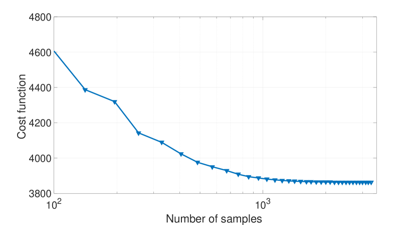
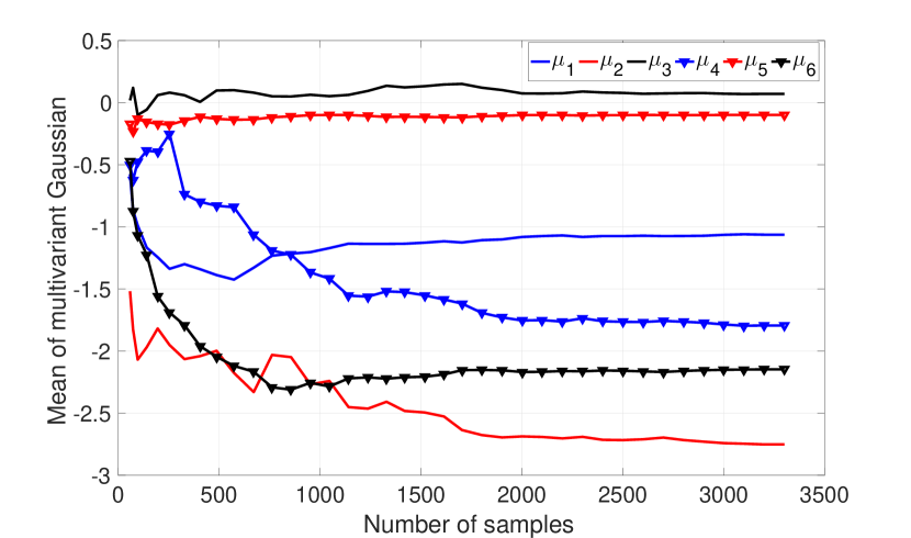
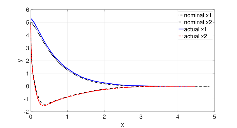
Figures 1(a) and 1(b) show the convergence result with SAOP in one simulation in terms of cost and the mean of the multivariant Gaussian over iterations. The following parameters are used: Initial sample size $N_{1}=50$, improvement parameter $\epsilon=0.1$, quantile percentage $\rho=0.1$, smoothing parameter $\lambda=0.5$, sample increment parameter $\alpha=0.1$.

The algorithm converges after $38$ iterations with $3301$ samples to the mean $\bar{w}^{\ast}=[-1.0629\;-2.7517\;0\;-1.7939\;-0.0987\;-2.1474]^{\intercal}$ and the covariance matrix with a norm $3.340110-04$. Each iteration took less than 10 seconds. The approximate optimal cost under feedback controller $u=\langle\bar{w}^{\ast},\phi\rangle$ is $3863.3$. Figure 1(c) shows the state trajectory for the closed-loop system with bounded disturbances. With 25 independent runs of SAOP, the mean of $J(x_{0};\bar{w}_{i}^{\ast}),i=1,\ldots,25$ is $3903.3$ and the standard deviation is $104.1683$, $2.6\%$ of the approximate optimal cost.

Note, if we only use linear feedback $u=Kx$, the optimal cost is $1.09431004$, which is about three times the optimal cost that can be achieved with a nonlinear controller.

0.4.2 Example: approximate optimal planning of a Dubins car

Consider a Dubins car dynamics

$$\dot{x}=u\cos\theta,\quad\dot{y}=u\sin\theta\;\quad\dot{\theta}=v$$

where $\vec{x}=(x,y,\theta)\in\mathbf{R}^{2}\times\mathbb{S}^{1}$ being the state (coordinates and turning angle with respect to $x$-axis) and $u$ and $v$ are control variables including linear and angular velocities. The system is kinematically constrained by its positive minimum turning radius $r$ which implies the following bound $\lvert v\rvert\leq\frac{1}{r}$. Without loss of generality, we assume $\lvert v\rvert\leq 5$ and $\lvert u\rvert\leq 10$ are the input constraints. The control objective is to reach the goal $x_{f}=20,y_{f}=20$ while avoiding static obstacles. The cost function $J=\int_{0}^{T}\ell(x,u)dt+g(x,u)$ where $T=100$, the running cost is $\ell(x,u)=0.1\times(\lVert x\rVert+\lVert u\rVert)$, and the terminal cost is $g(x(T),u(T))=1000\times\lVert(x(T),y(T))-(x_{f},y_{f})\rVert$. The initial state is $\vec{x}_{0}=\mathbf{0}$. In simulation, we consider the robot reaches the target if $\lVert(x,y)^{\prime}-(x_{f},y_{f})\rVert\leq\varepsilon$ for $\varepsilon\in[0,1]$. In simulation, $\varepsilon=0.5$.

We select RBF as basis functions and define $\phi_{rbf}=[\phi_{1},\ldots,\phi_{N}]^{\intercal}$ for $N$ center points. In the experiment, the center points are includes 1) uniform grids in $x-y$ coordinates with step sizes $\delta x=5$, $\delta y=5$; and 2) vertices of the obstacle. We also include linear basis functions $\phi_{linear}=[(x-x_{f}),(y-y_{f}),\theta]$. The basis vector is $\phi=[\phi_{rbf}^{\intercal},\phi_{linear}^{\intercal}]^{\intercal}$. We consider a bounded domain $-5\leq x\leq 30$ and $-5\leq y\leq 30$ and $\theta\in[0,2\pi]$ and thus the total number of basis functions is $80$. The control input $\vec{u}=[u,v]^{\intercal}$ where $u=w_{u}^{\intercal}\phi$ and $v=w_{v}^{\intercal}\phi$. The total number of weight parameters is twice the number of bases and in this case $160$.

(a)

(b)

Figure 2: Convergence of the the planning algorithm algorithm on the Dubins car. (a) The planned trajectory under feedback policy $\langle\mu,\phi\rangle$ computed using the mean of multivariate Gaussian over iterations (from the lightest to the darkest). (b) The convergence of the covariance matrix. (c) The total cost evaluated at the mean of the multivariate Gaussian over iterations.

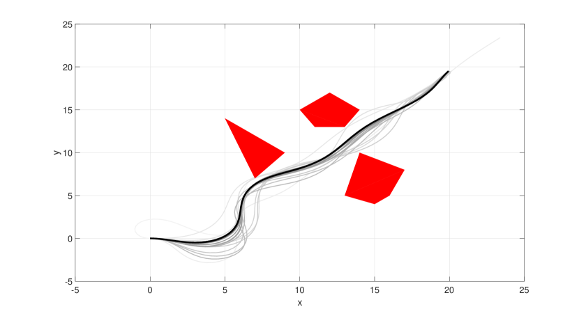
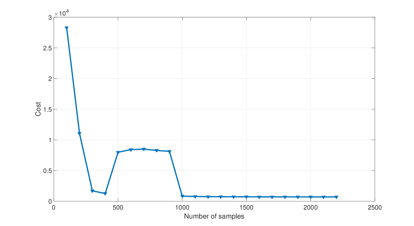
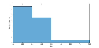
The following parameters are used: Initial sample size $N_{1}=100$, improvement parameter $\epsilon=0.1$, smoothing parameter $\lambda=0.5$, sample increment percentage $\alpha=0.1$, and $\rho=0.1$. In Fig. 2(a) we show the trajectory computed using the estimated mean of multivariate Gaussian distribution over iterations, from the lightest ($1$-th iteration) to the darkest (the last iteration when stopping criterion is met). The optimal trajectory is the darkest line. In Fig. 2(b) we show the cost computed using the mean of multivariate Gaussian over iterations. SAOP converges after 22 iterations with $2200$ samples and the optimal cost is $697.29$. Each iteration took about $20$ to $30$ seconds. However, it generates a collision-free path only after $5$ iterations. Due to input saturation, the algorithm is only ensured to converge to a local optimum. However, in 24 independent runs, all runs converges to a local optimum closer to the global one, as shown in the histogram in Fig. 3. Our current work is to implement trajectory-based contraction analysis using time-varying matrices $M(x,t)$ and adaptive bound $\beta$, which are needed for nonlinear Dubins car dynamics.

Figure 3: The frequency distribution of the optimal costs with 24 independent runs.

0.5 Conclusion

In this paper, an importance sampling-based approximate optimal planning and control method is developed. In the control-theoretic formulation of optimal motion planning, the planning algorithm performs direct policy computation using simulation-based adaptive search for an optimal weight vector corresponding to an approximate optimal feedback policy. Each iteration of the algorithm runs time linear in the number of samples and in the time horizon for simulated runs. However, it is hard to quantify the number of iterations required for MRAS to converge. One future work is to consider incorporate multiple-distribution importance sampling to achieve faster and better convergence results. Based on contraction analysis of the closed-loop system, we show that by modifying the sampling-based policy evaluation step in the algorithm, the proposed planning algorithm can be used for joint planning and robust control for a class of nonlinear systems under bounded disturbances. In future extension of this work, we are interested in extending this algorithm for stochastic optimal control.

Bibliography

- [1] S. M. LaValle, Planning algorithms. Cambridge university press, 2006.
- [2] L. E. Kavraki, P. Svestka, J.-C. Latombe, and M. H. Overmars, “Probabilistic roadmaps for path planning in high-dimensional configuration spaces,” IEEE transactions on Robotics and Automation, vol. 12, no. 4, pp. 566–580, 1996.
- [3] S. M. Lavalle, “Rapidly-exploring random trees: A new tool for path planning,” Iowa State University, Tech. Rep., 1998.
- [4] S. Karaman and E. Frazzoli, “Sampling-based algorithms for optimal motion planning,” The International Journal of Robotics Research, vol. 30, no. 7, pp. 846–894, 2011.
- [5] D. P. Bertsekas, “Approximate policy iteration: A survey and some new methods,” Journal of Control Theory and Applications, vol. 9, no. 3, pp. 310–335, 2011.
- [6] ——, “Dynamic programming and optimal control 3rd edition, volume ii,” Belmont, MA: Athena Scientific, 2011.
- [7] M. Abu-Khalaf and F. L. Lewis, “Nearly optimal control laws for nonlinear systems with saturating actuators using a neural network hjb approach,” Automatica, vol. 41, no. 5, pp. 779–791, 2005.
- [8] D. P. Bertsekas and J. N. Tsitsiklis, Neuro-dynamic programming. Athena Scientific, 1996.
- [9] J. Hu, M. C. Fu, and S. I. Marcus, “A model reference adaptive search method for global optimization,” Operations Research, vol. 55, no. 3, pp. 549–568, 2007.
- [10] T. Homem-de Mello, “A study on the cross-entropy method for rare-event probability estimation,” INFORMS Journal on Computing, vol. 19, no. 3, pp. 381–394, 2007.
- [11] M. Kobilarov, “Cross-entropy randomized motion planning,” Robotics: Science and Systems VII, p. 153, 2012.
- [12] S. C. Livingston, E. M. Wolff, and R. M. Murray, “Cross-entropy temporal logic motion planning,” in Proceedings of the 18th International Conference on Hybrid Systems: Computation and Control. ACM, 2015, pp. 269–278.
- [13] D. P. Bertsekas, Dynamic programming and optimal control. Athena Scientific Belmont, MA, 1995, vol. 1, no. 2.
- [14] M. Hauschild and M. Pelikan, “An introduction and survey of estimation of distribution algorithms,” Swarm and Evolutionary Computation, vol. 1, no. 3, pp. 111–128, 2011.
- [15] W. Lohmiller and J.-J. E. Slotine, “On contraction analysis for non-linear systems,” Automatica, vol. 34, no. 6, pp. 683–696, 1998.
- [16] X. Liu, Y. Shi, and D. Constantinescu, “Robust constrained model predictive control using contraction theory,” in IEEE Conference on Decision and Control, Dec 2014, pp. 3536–3541.