Fork Tensor Product States - Efficient Multi-Orbital Real Time DMFT Solver

Abstract

We present a tensor network especially suited for multi-orbital Anderson impurity models and as an impurity solver for multi-orbital dynamical mean-field theory (DMFT). The solver works directly on the real-frequency axis and yields high spectral resolution at all frequencies. We use a large number $\left(\mathcal{O}(100)\right)$ of bath sites, and therefore achieve an accurate representation of the bath. The solver can treat full rotationally-invariant interactions with reasonable numerical effort. We show the efficiency and accuracy of the method by a benchmark for the three-orbital testbed material SrVO3. There we observe multiplet structures in the high-energy spectrum which are almost impossible to resolve by other multi-orbital methods. The resulting structure of the Hubbard bands can be described as a broadened atomic spectrum with rescaled interaction parameters. Additional features emerge when $U$ is increased. Finally we show that our solver can be applied even to models with five orbitals. This impurity solver offers a new route to the calculation of precise real-frequency spectral functions of correlated materials.

I Introduction

Strongly correlated systems are among the most fascinating objects solid-state physics has to offer. The interactions between constituents of such systems lead to emergent phenomena that cannot be deduced from the properties of non-interacting particles Anderson (1972).

One of the most widely used methods to describe strongly-correlated electrons is the dynamical mean-field theory (DMFT) Georges et al. (1996); Metzner and Vollhardt (1989). DMFT treats local electronic correlations by a self-consistent mapping of the lattice problem onto an effective Anderson impurity model (AIM). Calculating the single particle spectral function of this impurity model in an accurate and efficient way is at the heart of every DMFT calculation. To this end, many numerical methods have been developed or adapted. These are based for instance on continuous-time quantum Monte Carlo (CTQMC) Gull et al. (2011); Werner et al. (2006), exact diagonalization (ED) Caffarel and Krauth (1994); Capone et al. (2007); Kolorenč et al. (2015), the numerical renormalization group (NRG) Wilson (1975); Bulla et al. (2008), configuration interaction (CI) based solver Lu et al. (2014); Zgid et al. (2012), and also the density-matrix renormalization group (DMRG) with matrix-product states (MPS) White (1992); Schollwöck (2011).

Every algorithm has strengths and weaknesses: CTQMC is exact apart from statistical errors on the imaginary axis and can deal with multiple orbitals, but it is in some cases plagued by the fermionic sign problem. Additionally, an ill-posed analytic continuation is necessary to obtain real-frequency spectra, which therefore become broadened, especially at high energies. ED directly provides spectra on the real axis, but it is severely limited in the size of the Hilbert space, i.e. in the number of bath sites. Quite recently, NRG was shown to be a viable three-band solver by exploiting non-abelian quantum number conservation Stadler et al. (2015); Horvat et al. (2016); Stadler et al. (2016). NRG works on the real axis and captures the low-energy physics well, but it has by construction a poor resolution at higher energies. Another interesting route that has been proposed recently are solvers that tackle the problem of exponential growth of the Hilbert space using ideas from quantum chemistry, i.e. the configuration interaction Lu et al. (2014); Zgid et al. (2012). They allow to go beyond the small bath sizes of ED, keeping all the advantages such as absence of fermionic sign problems. However, in multi-orbital applications (see Appendix of Ref. Zgid et al. (2012)), the spectral resolution has so far been restricted by the restricted number of bath sites ($\mathcal{O}(20)$).

MPS based techniques like DMRG, finally, do not suffer from a sign problem and can be used on the real- as well as on the imaginary-frequency axis. The price to pay for the absence of the sign problem is an, in general, very large growth of bond dimension with the number of orbitals.

Dynamical properties and spectral functions can be calculated within DMRG and have been used for impurity solvers, e.g. with the Lanczos-like continued-fraction expansion Hallberg (1995); García et al. (2004). Other solvers using the more stable correction vector Kühner and White (1999) and dynamical DMRG (DDMRG) Jeckelmann (2002) methods were developed Nishimoto and Jeckelmann (2004); Peters (2011); Karski et al. (2008, 2005). Both algorithms produce very accurate spectral functions, but have the disadvantage that a separate calculation for each frequency has to be performed. The Chebyshev expansion Weiße et al. (2006) with MPS Holzner et al. (2011), supplemented by linear prediction White and Affleck (2008), was used for impurity solvers in the single band case Ganahl et al. (2014) and for two bands Wolf et al. (2014a). Recently, some of us introduced a method based on real-time evolution Vidal (2003, 2004); White and Feiguin (2004); Daley et al. (2004) and achieved a self consistent DMFT solution for a two-band model Ganahl et al. (2015). In such calculations, the physical orbitals for each spin direction are usually combined to one large site in the MPS. Three or more orbitals have not been feasible with this approach, because of a large increase in computational cost with the number of orbitals. Another MPS-based solver, which works on the imaginary axis, was recently introduced Wolf et al. (2015) and it was applied as a solver for three bands in two-site cluster DMFT. It was supplemented by a single real-time evolution to compute the spectral function, avoiding the analytic continuation. However, this method is restricted by the number of bath sites which can be employed. In the calculation mentioned, only three bath sites per orbital were used, limiting the energy resolution for real-frequency spectral functions.

In the present paper, we introduce a novel impurity solver which works directly on the real-frequency axis. To this end, we use a tensor network that captures the geometry of the interactions in the Anderson model better than a standard MPS. Our approach is to some extent inspired by the work of Ref. Holzner et al. (2010), which used a similar network for a two orbital NRG ground state calculation. We are not restricted to a small number of bath sites. This is imperative for exploiting the spectral resolution achievable with real-time calculations. We emphasize that (i) our method is by construction free of any fermionic sign problem, (ii) one can fully converge the DMFT self-consistency loop on the real-frequency axis and (iii) we can achieve an almost exact representation of the bath spectral function. We apply this method to multi-orbital DMFT for the testbed material SrVO3 and show that one can resolve a multiplet structure in the Hubbard bands, keeping at the same time a good description of the low-energy quasi-particle excitations.

The paper is structured as follows. First we show how impurity solvers with tensor networks work in general and introduce our new tensor network approach which we call fork tensor-product states (FTPS) (Sec. II). Next we explain in detail how our solver is used in the context of multi-orbital DMFT (Sec. III). In Sec. IV, we apply our approach to SrVO3 and discuss the multiplet structure that the FTPS solver allows to resolve. In order to check the accuracy of the method, we also compare the FTPS results to CTQMC for SrVO3. Finally, we show the efficiency of the FTPS solver by applying it to a five-orbital model.

II Tensor Network Impurity Solvers

The Anderson impurity model (AIM) describes an impurity (with Hamiltonian $H_{\text{loc}}$) coupled to a bath of non-interacting fermions hybridized with it. A typical AIM Hamiltonian is given by:

$$H =H_{\text{loc}}+H_{\text{bath}}$$ (1)

$$H_{\text{loc}} =\epsilon_{0}\sum_{m\sigma}n_{m0\sigma}+H_{\text{DD}}+H_{\text{SF-PH}}$$

$$H_{\text{DD}} =U\sum_{m}n_{m0\uparrow}n_{m0\downarrow}$$

$$+(U-2J)\sum_{m^{\prime}>m,\sigma}n_{m0\sigma}n_{m^{\prime}0\bar{\sigma}}$$

$$+(U-3J)\sum_{m^{\prime}>m,\sigma}n_{m0\sigma}n_{m^{\prime}0\sigma}$$

$$H_{\text{SF-PH}} =J\sum_{m^{\prime}>m}\left(c_{m0\uparrow}^{{\dagger}}c_{m0\downarrow}c_{m^{\prime}0\uparrow}c_{m^{\prime}0\downarrow}^{{\dagger}}+\text{h.c.}\right)$$

$$-J\sum_{m^{\prime}>m}\left(c_{m0\uparrow}^{{\dagger}}c_{m0\downarrow}^{{\dagger}}c_{m^{\prime}0\uparrow}c_{m^{\prime}0\downarrow}+\text{h.c.}\right)$$

$$H_{\text{bath}} =\sum_{ml\sigma}\epsilon_{l}n_{ml\sigma}+V_{l}\left(c_{m0\sigma}^{{\dagger}}c_{ml\sigma}+\text{h.c.}\right),$$

where $c_{ml\sigma}^{{\dagger}}$ ($c_{ml\sigma}$) creates (annihilates) an electron in band $m$ ($m\in\{1,2,3\}$ for a three-orbital model) with spin $\sigma$ at the $l$-th site of the system (the impurity has index $l=0$, the bath degrees of freedom have $l\geq 1$), and $n_{ml\sigma}$ are the corresponding particle number operators. $H_{\text{DD}}$ describes density-density (DD) interactions between all orbitals and $H_{\text{SF-PH}}$ are the spin-flip and pair-hopping terms. This three-orbital Hamiltonian is not only important in the context of real-material calculations. It has also been studied extensively on the model level, most importantly because it hosts unconventional correlation phenomena. For a selection of recent work, see for instance Refs. Werner et al. (2008); Stadler et al. (2015); de’ Medici et al. (2011); Georges et al. (2013); Kim et al. (2017).

An impurity solver calculates the retarded impurity Greens function $G(t)$

$$G(t)=-i\theta(t)\bra{\psi_{0}}[c^{{\dagger}}(t),c(0)]\ket{\psi_{0}}$$ (2)

of the interacting problem (1), either in real or imaginary time $t$. In the present paper, we introduce a new tensor network similar to an MPS, which can be used as a real-time impurity solver for three orbitals. We first introduce MPS before moving on to what we call fork tensor-product states (FTPS) in Sec. II.2.

II.1 Matrix Product States (MPS) and DMRG

MPS are a powerful tool to efficiently encode quantum mechanical states. Consider a state $\ket{\psi}$ of a system consisting of $N$ sites:

$$\ket{\psi}=\sum_{s_{1},s_{2},\cdots,s_{N}}c_{s_{1},\cdots,s_{N}}\ket{s_{1},s_{2},\cdots,s_{N}}\text{.}$$ (3)

Each site $i$ has a local Hilbert space of dimension $d_{i}$ spanned by the states $\ket{s_{i}}$. Through repeated use of singular-value decompositions (SVDs), it is possible to factorize every coefficient $c_{s_{1},\cdots,s_{N}}$ into a product of matrices Schollwöck (2011), i.e. into an MPS,

$$\ket{\psi}=\sum_{s_{1},s_{2},\cdots,s_{N}}A_{1}^{s_{1}}\cdot A_{2}^{s_{2}}\cdots A_{N}^{s_{N}}\ket{s_{1},s_{2},\cdots,s_{N}}.$$ (4)

Each $A_{i}^{s_{i}}$ is a rank-3 tensor, except the first and last ones ($A_{1}^{s_{1}}$, $A_{N}^{s_{N}}$), which are of rank two. The index $s_{i}$ is called physical index, and the matrix indices, which are summed over, are the so called bond indices. A general state of the full Hilbert space is unfeasible to store, but it can be shown that ground states are well described by an MPS with limited bond dimension $m$ (dimension of the bond index) Verstraete and Cirac (2006).

In complete analogy to the states, one can factorize an operator into what is called a matrix-product operator (MPO) Schollwöck (2011),

$$H=\sum_{\begin{subarray}{c}s_{1},\cdots,s_{N}\\ s_{1}^{\prime},\cdots,s_{N}^{\prime}\end{subarray}}W_{1}^{s_{1},s_{1}^{\prime}}\cdots W_{N}^{s_{N},s_{N}^{\prime}}\ket{s_{1}^{\prime},\cdots,s_{N}^{\prime}}\bra{s_{1},\cdots,s_{N}},$$ (5)

where each $W_{i}^{s_{i},s_{i}^{\prime}}$ is a rank-4 tensor. Tensor networks in general have a very useful graphical representation, which is shown for an MPS and an MPO in Fig. 1. Note that when we use the term MPS we always mean a one-dimensional chain of tensors as shown in Fig. 1.

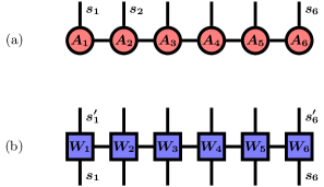
Figure 1: (a) Graphical representation of an MPS. Every circle corresponds to a tensor $A_{i}^{s_{i}}$ and each line to an index of this tensor. In this picture, the physical indices are the vertical lines, while the horizontal lines show the bond indices. Connected lines mean that the corresponding index is summed over. Fixing all the physical indices $s_{i}$ for each site results in a tensor of rank zero with the value of the coefficient $c_{s_{1},\cdots,s_{N}}$.
(b) Graphical representation of an MPO. The difference to an MPS is that an MPO has incoming indices $s_{i}$ and outgoing indices $s_{i}^{\prime}$ corresponding to the bra- and ket vectors of the operator.

To calculate Greens functions within the MPS formalism, one usually first applies the DMRG White (1992); Schollwöck (2011), which acts on the space of MPS and finds a variational ground state $\ket{\psi_{0}}$ and ground-state energy $E_{0}$. It minimizes the expectation value

$$E_{0}=\min_{\ket{\psi}}\frac{\braket{\psi}{H}{\psi}}{\braket{\psi}{\psi}}$$ (6)

by updating usually two neighboring MPS tensors before moving on to the next bond. This procedure also yields the Schmidt decomposition of the state at the current bond on the fly. The DMRG approximation is to keep only those states with the largest Schmidt coefficient. It is important to note that one can perform a DMRG calculation for any tensor network, as long as one can generate a Schmidt decomposition Murg et al. (2010).

For obtaining the Greens function, we employ an evolution in real time. Eq. (2) is split into the greater $G^{>}$ and lesser Greens function $G^{<}$:

$$G(t) =-i\Theta(t)\bigg{(}G^{>}(t)+G^{<}(t)\bigg{)}$$

$$G^{>}(t) =\braket{\psi_{0}}{ce^{-iHt}c^{\dagger}}{\psi_{0}}e^{iE_{0}t}$$

$$G^{<}(t) =\braket{\psi_{0}}{c^{\dagger}e^{iHt}c}{\psi_{0}}e^{-iE_{0}t}\text{,}$$ (7)

which are calculated in two separate time evolutions. This is done by first applying $c^{\dagger}$ (or $c$) and then time evolving this state and calculating the overlap with the state at time $t=0$. The time evolution is the most computationally expensive part, since time evolved states are not ground states anymore, and the needed bond dimensions usually grow very fast with time.

II.2 Fork Tensor Product States (FTPS)

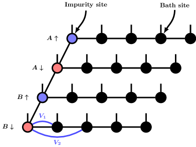
Figure 2: Graphical representation of a fork tensor product state (FTPS) for multi-orbital AIM. The idea to separate bath degrees of freedom leads to a fork-like structure. In this picture, a two-orbital model with four bath sites each is shown. Orbitals are labeled $A$ and $B$ and the arrows denote the spin. Each spin-orbital combination has its own bath sticking out to the right. As in Fig. 1, the vertical lines are the physical degrees of freedom (all of dimension two, for empty, resp. occupied bath sites). All other lines are bond indices and like in the MPS they are summed over. As mentioned in the text, the bath is represented in star geometry due to the smaller bond dimensions needed. The bath sites are ordered according to their on-site energies. Two example hoppings $V_{1}$ and $V_{2}$ are drawn.

So far, the usual way of dealing with Hamiltonians like Eq. (1) using MPS Ganahl et al. (2015, 2014); Wolf et al. (2014a) has been to place the impurity in the middle of the system and the up- and down-spin degrees of freedom to its left and right, resp. The local state space of each bath site then consists of $M$ spinless-fermion degrees of freedom, with dimension $2^{M}$, where $M$ is the number of orbitals in the Hamiltonian Eq. (1). This exponential growth is usually accompanied by a very fast growth in bond dimension when using the above arrangement. We did indeed encounter this very fast growth upon calculating the ground state of some one- two- and three-orbital test cases.

For treatment by MPS, the general Hamiltonian Eq. (1) with hopping terms from the impurity to each bath site is usually transformed into a Wilson chain with nearest-neighbor hoppings only, i.e.  of the form $t_{i}(c_{i}^{\dagger}c_{i+1}+\text{h.c.})$ Bulla et al. (2008). This was thought to be necessary since long-range interactions look problematic for MPS-based algorithms. Quite recently, though, it was discovered that MPS can deal with the original form of $H_{\rm bath}$ in Eq. (1) better Wolf et al. (2014b). Because all hopping terms in $H_{\rm bath}$ originate from the impurity, this is called the star geometry. The reason for the better performance is that in the star geometry one has many nearly fully occupied (empty) bath sites with very low (high) on-site energies $\epsilon_{l}$.

Since basis states with many unoccupied low-energy sites have a very low Schmidt coefficient, these states are discarded from the MPS. The same holds for occupied high energy sites. However, when dealing with multi-orbital models, the star geometry is not enough to be able to calculate Greens functions using MPS. The growth of the bond dimensions still makes those calculations unfeasible.

The key idea of the present work is to construct a tensor network which is beyond a standard MPS, but similar enough to be able to use established methods like DMRG and time evolution. From Hamiltonian (1) one can immediately notice that there are no terms coupling bath sites of different orbitals. Hence, it might not be advantageous to combine those, not directly interacting, degrees of freedom into one large physical index in the MPS.

Our proposed tensor network, therefore, separates the bath degrees of freedom as much as possible. It consists of separate tensors for every orbital-spin combination, each connected to bath tensors as shown in Fig. 2. This tensor network is no MPS anymore, since there are some tensors (labeled $A\downarrow$ and $B\uparrow$ in the example of Fig. 2) that have three bond indices and one physical index, i.e. which are of rank 4. Cutting any bond splits the network into two separate parts. Therefore, one can calculate the Schmidt decomposition in a way very similar to an MPS, which means that also DMRG is possible. The main bottleneck of calculations with FTPS is to perform SVDs of the rank-4 tensors representing the impurities. When all bond indices have the same dimension $\chi$, it is necessary to do a SVD for a $\chi^{2}d\times\chi$ matrix with computational complexity $\mathcal{O}(\chi^{4}d)$. However, as we show below, this operation does not pose a substantial problem for calculations using FTPS. Since the impurity tensors pose the biggest challenge, our tensor network would likely also allow us to deal with the chain geometry without a drastic increase in computational cost. In the present paper we will only use FTPS with baths in star geometry.
The proposed FTPS are similar to the tensor network used by Holzner et al. Holzner et al. (2010) to perform NRG calculations for ground state properties of an AIM with two orbitals.

The three-legged tensors in our network (Fig. 2) can also be interpreted as two coupled junctions with three legs in the language of Ref. Guo and White (2006), where it has been shown that DMRG is possible on such junctions. Furthermore, our approach has similarities with the so called Tree Tensor Networks (TTN) Shi et al. (2006); Tagliacozzo et al. (2009); Murg et al. (2010); Pižorn et al. (2013).

II.2.1 Time Evolution

Time evolution with the Hamiltonian Eq. (1) is not straightforward, since it features long-range hoppings. Possible methods include Krylov approaches Schmitteckert (2004), the time-dependent variational principle Haegeman et al. (2011, 2016) and the series expansion of $e^{iHt}$ proposed by Zaletel et al. Zaletel et al. (2015). In this work, however, we use a much simpler approach.

First, we split the Hamiltonian into the following terms: (i) the spin-flip and pair-hopping terms $H^{\text{SF-PH}}_{m,m^{\prime}}$ for each orbital combination, with $\sum_{m^{\prime}>m}H^{\text{SF-PH}}_{m,m^{\prime}}=H_{\text{SF-PH}}$ (see Eq. (1)), (ii) the density-density interaction terms $H_{\text{DD}}$, and (iii) all other terms $H_{\text{free}}=H_{\text{bath}}+\epsilon_{0}\sum_{m\sigma}n_{m0\sigma}$. With these terms, we write the time-evolution operator for a small time step $\Delta t$ using a second-order Suzuki-Trotter decomposition Suzuki (1990),

$$e^{-i\Delta tH} \approx\left(\prod_{m^{\prime}>m}e^{-i\frac{\Delta t}{2}H^{\text{SF-PH}}_{m,m^{\prime}}}\right)\cdot e^{-i\frac{\Delta t}{2}H_{\text{DD}}}\cdot$$

$$\times e^{-i\Delta tH_{\text{free}}}\cdot e^{-i\frac{\Delta t}{2}H_{\text{DD}}}\cdot\left(\prod_{m^{\prime}>m}e^{-i\frac{\Delta t}{2}H^{\text{SF-PH}}_{m,m^{\prime}}}\right)\text{.}$$ (8)

Note that in this decomposition, the order of the spin-flip and pair-hopping terms is important. The order of operators in the second product must be opposite to the one in the first.

We see that Eq. (8) involves three different operators $H^{\text{SF-PH}}_{m,m^{\prime}}$, $H_{\text{DD}}$ and $H_{\text{free}}$, each of which will be treated differently.

Time evolution of the density-density interactions is performed with an MPO-like representation of the time-evolution operator $e^{-i\frac{\Delta t}{2}H_{\text{DD}}}$. For a three-orbital model, first the full matrix ($4^{3}\times 4^{3}$) of $e^{-i\frac{\Delta t}{2}H_{DD}}$ is created, which is then decomposed into MPO-form by repeated SVDs. Since $H_{\text{DD}}$ only consists of density-density interactions, no fermionic sign appears in $e^{-i\Delta tH_{\text{DD }}}$.

Time evolution of the spin-flip and pair-hopping terms is more involved than the density-density interactions, since the operators change the particle numbers on the impurity sites. Therefore, it can be difficult to deal with the fermionic sign of the time evolution operator when the impurities are not next to each other in the fermionic order. It turns out that the spin-flip and the pair-hopping terms have the property $\hat{A}^{3}=\hat{A}$ individually, with $\hat{A}$ being either the spin-flip or the pair-hopping operator, resp. Furthermore they commute with each other allowing us to separate them without Trotter error. The time-evolution operator of $J\hat{A}$ is then given by:

$$e^{-i\Delta tJ\hat{A}}=\mathds{1}+\hat{A}^{2}\big{(}\cos\left(\Delta tJ\right)-1\big{)}-i\hat{A}\sin\left(\Delta tJ\right)\text{.}$$ (9)

For this operator, an MPO can be found for which the fermionic sign can easily be determined.

To time evolve the bath terms we use an iterative second-order Suzuki-Trotter breakup for each term in $H_{\text{free}}$. Neglecting orbital ($m$) and spin ($\sigma$) indices, the first step in this breakup is the following: $e^{-i\Delta t\sum_{l=1}^{N_{b}}H_{l}}\approx e^{-i\frac{\Delta t}{2}H_{1}}\cdot e^{-i\Delta t\sum_{l=2}^{N_{b}}H_{l}}\cdot e^{-i\frac{\Delta t}{2}H_{1}}$. Next we split off $H_{2}$ and iterate this procedure until we end up with

$$e^{-i\Delta tH_{\text{free}}}\approx\prod_{m\sigma}\Bigg{[}\Bigg{(} \prod_{l=1}^{N_{b}-1}e^{-i\frac{\Delta t}{2}H_{ml\sigma}}\Bigg{)}\cdot e^{-i\Delta tH_{mN_{b}\sigma}}$$

$$\cdot\Bigg{(}\prod_{l=N_{b}-1}^{1}e^{-i\frac{\Delta t}{2}H_{ml\sigma}}\Bigg{)}\Bigg{]}\text{,}$$ (10)

with $N_{b}$ the number of bath sites and $H_{ml\sigma}=\epsilon_{l}n_{ml\sigma}+V_{l}\left(c_{m0\sigma}^{{\dagger}}c_{ml\sigma}+\text{h.c.}\right)$. In the above equation, we neglected the term $\epsilon_{0}n_{m0\sigma}$ that we add to $H_{m1\sigma}$. Eq. (II.2.1) is a product of two-site gates (an operator acting non-trivially only on two sites) with one of the two sites always being the impurity. This means that those two sites are not nearest neighbors in the tensor network. To overcome this problem, we use so called swap gates Schollwöck (2011); Stoudenmire and White (2010). The two-site operator

$$S_{ij}=\delta_{s_{i},s_{j}^{\prime}}\delta_{s_{j},s_{i}^{\prime}}\cdot(-1)^{n_{i}n_{j}}$$ (11)

swaps the state of site $i$ ($s_{i}$ with occupation $n_{i}$) with the state of site $j$ ($s_{j}$ with occupation $n_{j}$). The factor $(-1)^{n_{i}n_{j}}$ gives the correct fermionic sign and is negative if an odd number of particles on site $i$ gets swapped with an odd number of particles on site $j$. To be more precise, the matrix representation of the swap gates used in this work is:

$$S_{ij}=\ket{00}\bra{00}+\ket{10}\bra{01}+\ket{01}\bra{10}-\ket{11}\bra{11}\text{.}$$ (12)

It turns out that every swap gate can be combined with an actual time evolution gate without additional computational time. For example, the first step in this time evolution would be to apply $e^{-i\frac{\Delta t}{2}H_{m1\sigma}}$. Immediately afterwards, even before the SVD (to separate the tensors again), the swap gate is applied so that the impurity and the first bath sites are swapped. By repeating this process one moves the impurity along its horizontal arm in Fig. 2. Because a second-order decomposition is used, now all time evolution gates except the one at site $N_{b}$ have to be applied again. But now, the impurity and bath site needs to be swapped before time evolution.

Note that the algorithm presented above cannot only be used to perform real-time evolutions, but it is applicable also to evolution in imaginary time simply by replacing $idt$ by $d\tau$.

III Multi orbital DMFT with FTPS

In this section we present details of our impurity solver.

We refer to Refs. Georges (2004); Georges et al. (1996) for DMFT in general, and to Refs. Lechermann et al. (2006); Kotliar et al. (2006) for DMFT in the context of realistic ab-initio calculations for correlated materials.

In the latter approach, called density-functional theory (DFT)+DMFT, the correlated subspace is described by a Hubbard-like Hamiltonian. Within DMFT, this model is mapped onto the AIM Hamiltonian (1). This mapping defines the bath hybridization function $\Delta(\omega)$ describing the influence of the surrounding electrons.

Since FTPS provide the Greens function of the AIM on the real-frequency axis, also the self-consistency loop is performed directly for real frequencies. For calculating the bath hybridization, we use retarded Greens functions with a finite broadening $\eta_{SC}$ in order to avoid numerical difficulties with the poles of the Greens function. Throughout this work, we use $\eta_{SC}=0.005$ eV.

The impurity solver calculates the self energy $\Sigma(\omega)$ of the AIM, given the bath hybridization function $\Delta(\omega)$ and the interaction Hamiltonian on the impurity. To this end, our solver performs the following steps, which are explained in more detail in the text below:

1. Obtain bath parameters $\epsilon_{l}$ and $V_{l}$ by a deterministic approach based on integration of the bath hybridization function $\Delta(\omega)$.

2. Calculate the ground state $\ket{\psi_{0}}$ and ground-state energy $E_{0}$ of the interacting problem.

3. Apply impurity creation or annihilation operators, and time evolve these states to determine the interacting Greens function ( Eq. (2) ).

4. Fourier transform Eq. (2) to obtain $G(\omega)$ and calculate the local self-energy,

   $$\Sigma(\omega)=G_{0}(\omega)^{-1}-G(\omega)^{-1}\text{.}$$ (13)

To perform step 1 we use

$$V_{l}^{2} =\int_{I_{l}}\left[-\frac{1}{\pi}\operatorname{Im}\Delta(\omega)\right]d\omega$$

$$\epsilon_{l} =\frac{1}{V_{l}^{2}}\int_{I_{l}}\omega\left[-\frac{1}{\pi}\operatorname{Im}\Delta(\omega)\right]d\omega\text{,}$$ (14)

similar to Refs. Bulla et al. (2008) (NRG) and Wolf et al. (2014b). Each interval $I_{l}$ corresponds to a bath site. This discretization can be interpreted as representing each interval $I_{l}$ as a delta peak at position $\epsilon_{l}$ and weight $V_{l}^{2}$. Sum rules for such discretization parameters can be found analytically Koch et al. (2008). In this work we choose the length of each interval such that the area of the bath spectral function $-\frac{1}{\pi}\operatorname{Im}\Delta(\omega)$ is approximately constant for each interval de Vega et al. (2015). For the case at hand, this discretization was found to be numerically more stable than using intervals of constant length. Unless stated otherwise, we use $N_{b}=109$ bath sites per orbital and spin. We note that this scheme is not restricted to diagonal hybridizations. In the general case of off-diagonal hybridizations the hybridization function is a matrix $\underline{\Delta}$. Therefore, instead of taking the imaginary part we can use the bath spectral function $\frac{i}{2\pi}(\underline{\Delta}-\underline{\Delta}^{\dagger})$. Similarly to Eq. (III), we represent each interval by one delta-peak for each orbital. For instance, fixing $\epsilon_{l}$ to the center of the interval, the hopping parameters $V_{l}$ can be found systematically from the Cholesky factorization of $\int_{I_{l}}\frac{i}{2\pi}(\underline{\Delta}-\underline{\Delta}^{\dagger})d\omega$. Most importantly, this scheme does not involve any fitting procedure on the Matsubara axis. A very similar approach was developed independently in Ref. Liu et al. (2016).

In step 2 we use a DMRG approach with the following parameters, unless specified otherwise. The truncated weight $t_{w}$ (sum of all discarded singular values of each SVD) is kept smaller than $10^{-8}$. When spin-flip and pair-hopping terms are neglected, we use an even smaller cutoff of $10^{-9}$. Note that, except in the five-band calculation, we do not restrict the bond dimensions by some hard cutoff (see Appendix .2).

During time evolution (step 3), we use a truncated weight of $t_{w}=2\cdot 10^{-8}$, or $10^{-8}$ with density-density interactions only. We time evolve to $t=16$ eV^-1, with a time step of $\Delta t=0.01$ eV^-1. Greens functions are measured every fifth time step. The time-evolution operator of $H_{\text{loc}}$ is applied using the zip-up algorithm Stoudenmire and White (2010). Afterwards the Greens functions are extrapolated in time using the linear prediction method White and Affleck (2008); Ganahl et al. (2015) up to $t=250$ eV^-1. Time evolution is split into two runs one forward and one backwards in time Barthel (2013) to be able to reach longer times.

In the Fourier transform to $\omega$-space (step 4), we use a broadening in the kernel $e^{i\omega t-\eta_{FT}|t|}$ of $\eta_{FT}=0.02$ eV to avoid cutoff effects remaining after the linear prediction. The influence of the linear prediction on our results is discussed in Appendix .1. We want to stress that although a calculation with full rotational symmetry is more demanding, the computational effort is still very feasible. With the parameters mentioned above one full DMFT-cycle takes about five hours on 16 cores.

To verify that our implementation of DMRG and time evolution produces correct results when used with our tensor network, we first compared Greens functions and ground-state energies for $U=J=0$ for several bath parameter sets. The next step of our testing was to include density-density interactions, one term at a time. For example, we only included $(U^{\prime}-J)n_{10\uparrow}n_{30\uparrow}$ and compared energy and Greens function to a standard one-orbital MPS solver. Finally, we also compared our method to the MPS two-band solver used in Ref. Ganahl et al. (2015). Indeed all tests performed produced correct energies and Greens functions.

IV Results

We performed DMFT calculations based on a band structure obtained from density functional theory (DFT) for the prototypical compound SrVO3, using the approximation of the Kanamori Hamiltonian (Eq. (1)). It has a cubic crystal structure with a nominal filling of one electron in the V-3d shell . Due to the crystal symmetry, the five orbitals of the V-3d shell split into two $e_{g}$ and three $t_{2g}$ orbitals. The latter form the correlated subspace. We performed the DFT calculation with Wien2k Blaha et al. (2001), and used 34220 k-points in the irreducible Brillouin zone in order to reach an energy resolution comparable with the $\eta_{SC}=0.005$ eV broadening.

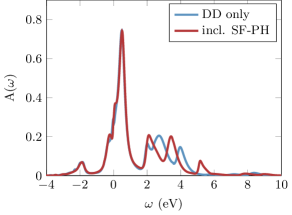
Figure 3: Spectral functions $A(\omega)$ for density-density interactions (DD) only (blue line), and with spin-flip and pair-hopping terms included (red line). In both calculations we used $U=4.0$ eV and $J=0.6$ eV. Both spectra show a three-peak structure in the upper Hubbard band and additional features at high energies (around $8$ eV).

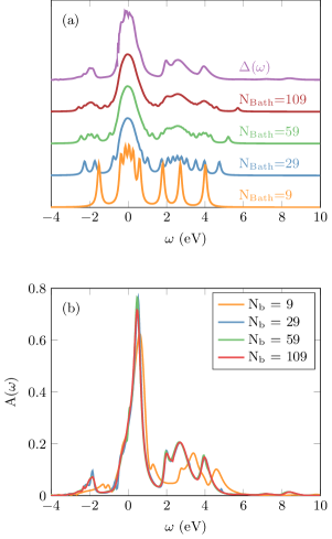
Figure 4: (a) We take the bath spectral function $\Delta(\omega)$ from the DMFT self-consistent solution for $N_{b}=109$ and represent it using various numbers of bath sites. It is obvious that $N_{b}=9$ is too small to represent the bath well. (b) Converged DMFT spectral function using the AIM with different numbers of bath sites. Only the smallest bath shows a noticeable difference. This is mostly due to the fact that in this case a higher broadening of $\eta_{FT}=0.1$ eV had to be used in the Fourier transform and time evolution was only possible to $t=14\text{ eV}^{-1}$. The additional small structure at $\omega=0$ for $N_{b}=59$ bath sites is most likely a linear prediction artifact.

The TRIQS/DFTTools package (v1.4) Aichhorn et al. (2016, 2009, 2011), which is based on the TRIQS library (v1.4) Parcollet et al. (2015), was used to generate the projective Wannier functions and to perform the DMFT self-consistency cycle.

Fig. 3 shows the main results of this paper, the DMFT spectral function $A(\omega)$ for SrVO3, (i) in the approximation of density-density interactions only and (ii) with full rotational invariance including spin-flip and pair-hopping terms. Overall, both cases show the well known features of the SrVO3 spectral function Liebsch (2003); Sekiyama et al. (2004). We see a hole excitation at around $-2$ eV, and the quasi-particle peak at zero energy whose shape and position does not depend on the inclusion of full rotational invariance. In the upper Hubbard band, a distinctive three-peak structure can be seen. This structure has not been resolved in other exact methods like CTQMC (problem with analytic continuation, see below) or NRG (logarithmic discretization problem). In our real time approach, high energies correspond to short times, where the calculations are particularly precise. Most methods allow to resolve structures in the Hubbard bands only in special cases (see Ref. Sangiovanni et al. (2006) for an example using ED). Of course, atomic-limit based algorithms such as the Hubbard-I approximation or non-crossing approximation (NCA) show atomic-like features, but they have very limited accuracy for the description of the low-energy quasi-particle excitations in the metallic phase Gull et al. (2010). Thus, our FTPS solver combines the best of the two worlds, with atomic multiplets at high energy and excellent low-energy resolution at the same time.

The energies of the three peaks in the upper Hubbard band differ depending on whether SF-PP terms are taken into account or not. Details of this peak structure, as well as additional excitations visible at higher energies, will be discussed below in Sec. IV.3.

First we examine the convergence of our results with respect to the number of bath sites and compare our spectrum to CTQMC. The following discussion is mostly based on calculations without spin-flip and pair-hopping terms. In this case, the calculations can be done faster and with higher precision, since there is no particle exchange between impurities. In all subsequent plots, we show results from calculations with DD interactions only.

IV.1 Effect of Bath Size

In order to achieve a reliable high resolution spectrum on the real-frequency axis, it is imperative to have a good representation of the hybridization function $\Delta(\omega)$ in terms of the bath parameters, for which a sufficient number of bath sites is needed. Fig. 4 shows how well a hybridization function can be represented with our approach (Eq. (III)) using a certain number of bath sites. We see that for $N_{b}=9$ bath sites (we always denote sites per orbital), $\Delta(\omega)$ can be reconstructed only very roughly, which in turn gives an incorrect spectral function (Fig. 4 bottom). To some extent, the difference in the spectrum is due to the shorter time evolution and therefore a higher broadening $\eta_{FT}$ we were forced to use. For such a small bath, the finite size effects from reflections at the bath ends appear much earlier in the time evolution.

Increasing the number of bath sites to $N_{b}=29$, we observe that the reconstructed bath spectral function already shows the relevant features of $\Delta(\omega)$. The spectrum is well converged for the largest bath sizes $N_{b}=59$ and $N_{b}=109$.

Figure 5: DMFT spectral functions $A(\omega)$ from CTQMC+MaxEnt (blue line) at $\beta=200$ eV^-1, and from FTPS (red line). The FTPS result shows a distinctive three-peaked structure in the upper Hubbard band.

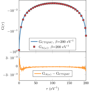
Figure 6: Comparison of imaginary time Greens functions $G(\tau)$ from CTQMC (G${}_{\text{CTQMC}}$, blue line) and FTPS using Eq. (15) ($\text{G}_{\text{A}(\omega)}$, red squares). The agreement is equally good also at $\beta=100$ eV^-1 and $\beta=400$ eV^-1 (not shown). The difference between the two Greens functions is shown in the bottom panel. Note that on both ends $\text{G}_{\text{A}(\omega)}$ is smaller than G${}_{\text{CTQMC}}$. The normalization of the spectral function demands that $G(\tau=0)+G(\tau=\beta)=-1$. The CTQMC data deviates in the order of $10^{-2}$ from this constraint due to statistical noise, while FTPS gives (by construction) the correct result to a precision of $10^{-8}$. This explains the bigger differences of the Greens functions around $\tau=0$ and $\tau=\beta$. For better visibility of the $\tau>0$ data, the value of $9\cdot 10^{-3}$ at $\tau=0$ is not shown.

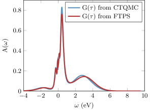
Figure 7: Spectral functions from analytically continued imaginary-time Greens functions $G(\tau)$ calculated by CTQMC (blue line) and by FTPS (red line). Clearly, the analytic continuation cannot resolve the peak structure in the upper Hubbard band.

IV.2 Comparison to CTQMC

In Fig. 5 we compare the converged spectral function of our approach (FTPS) with a spectrum obtained from CTQMC and analytic continuation. In both calculations, we used the same interaction Hamiltonian with density-density interactions only. The CTQMC calculation was performed with the TRIQS CTHYB-solver (v1.4) Seth et al. (2016); Werner and Millis (2006) with $3.2\cdot 10^{7}$ measurements and at inverse temperature $\beta=200$ eV^-1. For the analytic continuation we applied the $\Omega$MaxEnt method Bergeron and Tremblay (2016).

The three-peak structure in the upper Hubbard band is not present in the CTQMC spectrum. We will show below in an example that even for a Greens function that does contain these peaks the analytic continuation does not resolve this structure.

For another comparison, we consider the imaginary time Greens functions $G(\tau)$ in Fig. 6. Apart from the effect of statistical errors, CTQMC provides an exact self consistent solution of DMFT on the imaginary-frequency axis. As mentioned above, when we use the FTPS solver, we formulate the DMFT self-consistency equations on the real-axis. To obtain an approximate finite temperature imaginary-time Greens function from FTPS that we can compare to the CTQMC result, we need to take the finite temperature of the CTQMC calculation into account. Therefore, we use the FTPS spectrum $A(\omega)$ and assume that we would obtain the same spectrum for a finite (but high enough) inverse temperature $\beta$, and use:

$$G(\tau)=\int\frac{d\omega}{2\pi}A(\omega)\frac{e^{-\omega\tau}}{e^{-\beta\omega}+1}\text{}$$ (15)

The results in Fig. 6 show very good agreement on a logarithmic scale.

Another important indication of the validity of our results is the value of $A(\omega=0)$. To get a comparable number, we use the CTQMC imaginary time Greens function $G(\tau)$ and Fourier transform it to get $G(i\omega_{n})$:

$$G(i\omega_{n})=\int e^{i\omega_{n}\tau}G(\tau)d\tau\text{.}$$

Looking at the last few DMFT-cycles, we estimate it to be around $A(\omega=0)=-\frac{1}{\pi}\lim_{i\omega_{n}\to 0}\Im G(i\omega_{n})\approx 0.272$ eV^-1 with fluctuations in the last digit. For the FTPS, the exact height of $A(\omega=0)$ of the FTPS spectrum changes a little for each DMFT iteration, mainly due to slight variations in the linear prediction. Using the same prescription as for CTQMC, we estimate it to be $A(\omega=0)=0.28\text{ eV${}^{-1}$,}$ with fluctuations of about $0.01\text{ eV${}^{-1}$}$. This agreement is very good considering that linear prediction has its strongest influence at small energies. Further benchmarks concerning the linear prediction can be found in Appendix .1.

Finally, we show that the ill-posedness of the analytic continuation is the most likely explanation for the missing peak structure in the upper Hubbard band of the spectral function obtained from the CTQMC data. To do so, we take the FTPS spectrum $A(\omega)$, calculate $G(\tau)$ as described above, and perform the same analytic continuation that we did for the $G(\tau)$ from CTQMC. We added noise of the order of the CTQMC error to the FTPS data. The resulting spectrum is shown in Fig. 7, and indeed the peak structure in the upper Hubbard band vanishes.

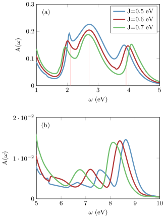
Figure 8: (a) Closeup of the three-peak structure for various values of $J$. Additionally, we show vertical lines for the $J=0.6$ eV spectrum at energies $\omega_{M}$ (position of the middle peak) and at $\omega_{M}+2J$ and $\omega_{M}-J$. We see that the width of the upper Hubbard band is close to $3J$. (b) Closeup of the small spectral peaks at high energies. These correspond to excitations into the $N=3$ sector of the atomic model (see Tab. 1). The height of each peak can be estimated by the degeneracy of the atomic states. Effective parameters $\bar{J}$ are $0.53$ eV ($J=0.5$ eV), $0.59$ eV ($J=0.6$ eV) and $0.68$ eV ($J=0.7$ eV). They are obtained from the difference between the two peaks highest in energy.

IV.3 Discussion of Peak Structure - Effective Atomic Physics

In order to understand the peak structure observed in the spectral functions, we take a look at the underlying atomic problem, where for simplicity we start with density-density interactions only. We will show that the same arguments hold for full rotationally invariant interactions.

Tab. 1 shows the relevant atomic states and their corresponding energies. The atomic model has a hole excitation at energy $-\epsilon_{0}$ and three single electron excitations with energies $U+\epsilon_{0}$, $U-2J+\epsilon_{0}$ and $U-3J+\epsilon_{0}$ relative to the ground state. If we measure the energy differences between the three peaks of the upper Hubbard band in our results, we find values of $1.27$ eV and $0.69$ eV, which is close to the atomic energy differences of $1.2$ eV and $0.6$ eV ($J=0.6$ eV). We also find the hole excitation at $-2.0$ eV. This indicates that we can describe the positions of the observed peaks approximately by atomic physics with effective parameters $\bar{\epsilon}_{0}$, $\bar{U}$ and $\bar{J}$ and widened peaks. Furthermore, the heights of the peaks roughly correspond to the degeneracy of the states in the atomic model (see Tab. 1).

Table 1: Relevant states of the atomic problem of Hamiltonian (1) without spin-flip and pair-hopping terms.

type	states	energy difference to ground state	degeneracy
$N=1$, ground state	$\ket{\uparrow,0,0}\text{ }\ket{\downarrow,0,0}\text{ }\ket{0,\uparrow,0}\cdots$	$0$	6
$N=0$	$\ket{0,0,0}$	$-\epsilon_{0}$	1
$N=2$, same spin	$\ket{\uparrow,\uparrow,0}\text{ }\ket{\uparrow,0,\uparrow}\text{ }\ket{0,\uparrow,\uparrow}\cdots$	$U-3J+\epsilon_{0}$	6
$N=2$, different spin	$\ket{\uparrow,\downarrow,0}\text{ }\ket{\uparrow,0,\downarrow}\text{ }\ket{\downarrow,\uparrow,0}\cdots$	$U-2J+\epsilon_{0}$	6
$N=2$, double occupation	$\ket{\uparrow\downarrow,0,0}\text{ }\ket{0,\uparrow\downarrow,0}\text{ }\ket{0,0,\uparrow\downarrow}$	$U+\epsilon_{0}$	3
$N=3$, all spins equal	$\ket{\uparrow,\uparrow,\uparrow}\text{ }\ket{\downarrow,\downarrow,\downarrow}$	$3U-9J+2\epsilon_{0}$	2
$N=3$, one spin different	$\ket{\uparrow,\uparrow,\downarrow}\text{ }\ket{\uparrow,\downarrow,\uparrow}\text{ }\ket{\downarrow,\uparrow,\uparrow}\cdots$	$3U-7J+2\epsilon_{0}$	6
$N=3$, double occupation	$\ket{\uparrow\downarrow,\uparrow,0}\text{ }\ket{\uparrow\downarrow,\downarrow,0}\text{ }\ket{\uparrow\downarrow,0,\uparrow}\cdots$	$3U-5J+2\epsilon_{0}$	12

We can determine $\bar{U}=5.97$ eV (where $U=4.00$ eV) from the energy difference of the peak highest in energy to the hole excitation. This increase of $\bar{U}$ compared to $U$ is plausible considering the following. When coupling the impurity to the bath, particles have the possibility to avoid each other by jumping into unoccupied sites of the bath. This results in a decrease of $\langle n_{\uparrow}n_{\downarrow}\rangle$. To model this situation using atomic physics, one needs to increase the interaction strength. Finally, it is well known that $J$ is much less affected by the surrounding electrons than $U$, since the latter is screened significantly stronger Vaugier et al. (2012).

Tab. 2 shows how bare atomic parameters change when adding a bath and we see that our qualitative arguments give a correct idea of how parameters are rescaled.

Table 2: Atomic parameters and their effective values obtained from the spectral functions shown in Fig. 5 and 8. For $J$ the values itself were obtained from the energy difference of the highest peak to the lowest peak, whereas the uncertainty is estimated from $\omega_{M}+2J$ and $\omega_{M}-J$.

parameter	atomic value (eV)	effective value (eV)
$\epsilon_{0}$	-$0.86$	-$2.00$
$U$	$4.00$	$5.97$
$J$	$0.50$	$0.59(6)$
$J$	$0.60$	$0.66(3)$
$J$	$0.70$	$0.72(2)$

Further evidence that the observed three-peaked structure is indeed a result of atomic physics can be seen in Fig. 8. It shows a closeup of the upper Hubbard band for three different values of $J$. The corresponding effective parameters $\bar{J}$ are shown in Tab. 2. We observe that also $J$ is rescaled slightly, but the rescaling gets smaller for higher $J$. Furthermore, increasing $J$ also increases the total width of the Hubbard band, which scales mostly linearly with $J$. At the same time, measuring the quasi-particle spectral weight as a function of $J$ at constant $U$ shows that it increases with increasing $J$, implying also an increasing critical $U_{c}$ for the metal-to-insulator transition Georges et al. (2013).

Upon a careful inspection of the spectral function in Fig. 5, we observe small peaks at energies around $8$ eV. A closeup of this energy region for different values of $J$ is shown in Fig. 8. The energy difference between the peaks is close to $2J$ and can, again, be well explained by atomic physics, namely excitations into states with 3 electrons on the impurity (Tab. 1) . These excitations originate from small admixtures of $N=2$ states to the ground state.

With atomic physics in mind, let us take a look again at the spectrum using full rotational symmetry (Fig. 3). The spin-flip and pair-hopping terms only contribute if there are two or more particles present. Thus, the quasi-particle peak and the hole excitation do not change. The atomic $N=2$ sector does change, however. Diagonalizing the Hamiltonian, we find eigenstates with three different energies and differences of $3J=1.8$ eV and $2J=1.2$ eV, resp. Measuring the energy differences in Fig. 3, we find $3\bar{J}=1.75$ eV and $2\bar{J}=1.32$ eV. Estimating $\bar{U}=5.81(5)$ we see that it does not change much compared to DD only. Again, we can describe the spectrum approximately by atomic physics with effective parameters. Like in the case with density-density terms only, we also see the tiny excitations to states belonging to the atomic $N=3$ sector.

IV.4 Beyond Atomic Physics

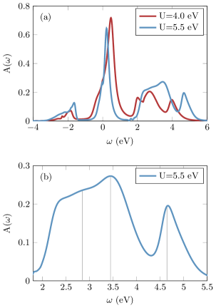
Figure 9: (a) Increasing $U$ results in a slimmer central peak and a shift of the upper Hubbard band. Also the three-peaked structure gets smeared out. (b) Closeup of the upper Hubbard band. As in Fig. 8, additional vertical lines are plotted at $\omega_{M}$ (position of the middle peak) and at $\omega_{M}+2J$ and $\omega_{M}-J$ as a rough guide to where the atomic peaks would be located. With the help of these lines one can discern a three-peaked structure again, but extended by a feature at the inside of the Hubbard band.

The previous section showed that at $U=4.0$ eV the spectral features in the Hubbard bands can be well described by atomic physics with effective parameters and widened peaks. It is not clear whether this picture is valid for higher interaction strengths $U$ in the metallic regime. In Fig. 9 we show results with $U=5.5$ eV at constant $J=0.6$ eV. We see a shift of the upper Hubbard band to higher energies, but little shift of the hole-excitation. Also the central peak is shifted and gets slimmer since more weight is transferred into the Hubbard bands. Most importantly, as we approach the strongly-correlated metallic regime, we clearly leave the realm where atomic physics can describe all the spectral features.

We find that the three-peak structure of the upper Hubbard bands smears out, and even vanishes. The closeup of the upper Hubbard band in Fig. 9 shows that with the help of the bare energy differences all three atomic peaks can be discerned again, accompanied by an additional structure at the low-energy side of the Hubbard band, which is reminiscent of the Hubbard side peaks found in the one- and two-band Hubbard model on the Bethe lattice Ganahl et al. (2015) upon increasing $U$. We leave further investigation of this feature to future work.

It might at first seem counter-intuitive that increasing $U$ makes the physics less atomic-like. Indeed, at very high interaction strengths, in the insulating regime, the spectrum must become atomic-like again. Here, however, we identify an intermediate regime where additional structures appear when increasing $U$, since we get closer to the Mott metal-to-insulator transition.

IV.5 Solution of a five-band AIM

In this section we show that FTPS can not only deal with three-band models, but also work in the case of five orbitals. To do so, we use the bath parameters $\epsilon_{k}$ and $V_{k}$ from the converged $N_{b}=59$ calculation for SrVO3 and construct an artificial degenerate five-band AIM. Interaction parameters are $U=4.0$ eV and $J=0.6$ eV. We decrease the on-site energy $\epsilon_{0}$ to get a similar occupation of each impurity orbital as for SrVO3 $(\langle n_{m,0,\sigma}\rangle\approx\frac{1}{6})$. Note that in doing so we have a model with, in total, $\frac{5}{3}$ electrons on the impurity. We only use density-density interactions and carry out the time evolution to $t=16$ eV^-1. We set the truncated weight to $t_{w}=10^{-8}$, but restrict the bond dimension of the impurity-impurity links to $\chi_{max}=200$.

In Fig. 10 we compare the results obtained for this five-band model to results from CTQMC, where we used the same discretized bath hybridization as input to CTQMC. We again see excellent agreement, even on a logarithmic scale. The spectrum $A(\omega)$ (not shown) again exhibits strong structure in the upper Hubbard band. Of course, the computational complexity is larger than in the three-orbital case and it grows during time evolution. Calculating the Greens function took about 190 hours on the processors specified in Appendix .2. We want to stress tough that the resulting spectrum (as well as Fig. 10) was already fully converged at $t=12$ eV^-1 (70 hours). We note that even with only one CPU hour ($t=6$ eV^-1) the resulting spectrum is almost converged and barely distinguishable from the final result. The benchmark therefore shows that with our FTPS approach a full five-orbital DMFT calculation is well within reach.

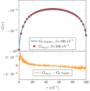
Figure 10: Comparison of imaginary time Greens functions $G(\tau)$ from CTQMC (G${}_{\text{CTQMC}}$, blue line) and FTPS using Eq. (15) ($\text{G}_{\text{A}(\omega)}$, red squares). As in Fig. 6 they compare very well.

V Conclusions

We have presented a novel multi-orbital impurity solver which uses a fork-like tensor network whose geometry resembles that of the Hamiltonian. The network structure is simple enough to generate Schmidt decompositions, allowing us to truncate the tensor network safely and to use established methods like DMRG and real time evolution. The solver works on the real frequency axis, and hence allows to formulate the full DMFT self consistency procedure for real frequencies. Therefore, results are not plagued by an ill-conditioned analytic continuation. Our approach exhibits no sign problem, tough it does become more involved for larger numbers of orbitals.

We tested the solver within DMFT on a Hamiltonian typically used for the testbed material SrVO3 and investigated the influence of full rotational invariance on the results. We found clear spectral structures in particular in the upper Hubbard band that have not been accessible by CTQMC, for which the necessary analytic continuation prohibits the resolution of fine structures in the spectral function at higher energies. For our calculations with $U=4.0$ eV, each peak in the spectrum corresponds to an atomic excitation. Even excitations into states with three particles on the impurity are resolved, as tiny spectral peaks at high energies. Furthermore, upon increasing $U$, an additional structure appears on the inside of the Hubbard bands, similar to the precursors of the sharp Hubbard side peaks found for the one- and two-band Hubbard models on the Bethe lattice Ganahl et al. (2015, 2014). We have also shown that our approch is feasible for five-orbital models, by comparing results from the FTPS solver to CTQMC for an artificial five-band model.

Appendix

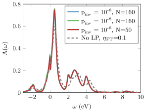
Figure 11: Spectrum $A(\omega)$ using different linear prediction (LP) parameters for a calculation without spin-flip and pair-hopping terms. The calculations with LP were performed with a broadening of $\eta_{FT}=0.02$  eV. Except for small changes around $\omega=0$, the effect of the various LP parameters is minor. The blue line directly lies below the red and green line. We also show a DMFT calculation without any LP. Even then the main features are still present.

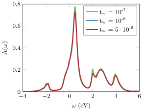
Figure 12: Different truncation values $t_{w}$ in the time evolution do not influence the shape of the spectrum $A(\omega)$.

In this appendix we show that our results are very stable over a wide range of computational parameters. First we focus on the linear prediction method (Sec. .1). Then we show that the results are converged with respect to the usual MPS-approximation (Sec. .2).

.1 Linear Prediction

In order to obtain smooth and sharp spectra, we used linear prediction (LP) to extrapolate the Greens function in time White and Affleck (2008); Ganahl et al. (2015). Without going into detail, we state the fact that linear prediction has two parameters, the pseudo inverse cutoff $p_{\text{inv}}$ and the order $N$ of the linear prediction. Fig. 11 shows that the results are converged in these parameters.

We also show a DMFT run without any linear prediction, which is only possible if we increase the broadening parameter of the Fourier transform to $\eta_{FT}=0.1$ eV, since otherwise we would get oscillations due to the hard cutoff of the time series. Except for a shift towards the right, omitting the linear prediction only changes the height (and width) of the peaks, but not the overall structure. This is a strong indicator of the stability of these features.

.2 Truncation of the Tensor Network

One, if not the most important, parameter in any MPS-like calculation is the sum of discarded singular values in each SVD (truncated weight $t_{w}$). We want to emphasize that this parameter is the only approximation in the representation of a state as a tensor-product state, as we do not impose any hard cutoff on the bond dimensions. Fig. 12 shows that the spectrum is well converged with respect to the truncation error during time evolution.

Finally, we want to comment on the required computational effort. In the calculation without full rotational symmetry, the size of the largest tensor to represent the ground state was $35\times 22\times 9\times 2$ ($t_{w}=10^{-9}$) and at the end of time evolution $127\times 79\times 30\times 2$ ($t_{w}=10^{-8}$). For a truncated weight of $t_{w}=10^{-7}$, calculating the Greens function took about 17 minutes on a node with two processors (Intel Xeon E5-2650v2, 2.6 GHz with 8 cores, and $G^{>}$ and $G^{<}$ each calculated on one processor). This time increases to five hours for the lowest truncated weight of $t_{w}=5\cdot 10^{-9}$. Using the full rotationally invariant Hamiltonian, the biggest tensor in the ground-state search was $90\times 40\times 10\times 2$ ($t_{w}=10^{-8}$) and at the end of time evolution $79\times 46\times 21\times 2$ ($t_{w}=2\cdot 10^{-8}$). The Greens function takes about three hours, and we need five hours for one full DMFT-cycle on the same two processors as above.

References

- Anderson (1972) P. W. Anderson, “More Is Different,” Science 177, 393–396 (1972).
- Georges et al. (1996) A. Georges, G. Kotliar, W. Krauth, and M. J. Rozenberg, “Dynamical mean-field theory of strongly correlated fermion systems and the limit of infinite dimensions,” Rev. Mod. Phys. 68, 13–125 (1996).
- Metzner and Vollhardt (1989) W. Metzner and D. Vollhardt, “Correlated Lattice Fermions in Dimensions,” Phys. Rev. Lett. 62, 324–327 (1989).
- Gull et al. (2011) E. Gull, A. J. Millis, A. I. Lichtenstein, A. N. Rubtsov, M. Troyer, and P. Werner, “Continuous-time Monte Carlo methods for quantum impurity models,” Rev. Mod. Phys. 83, 349–404 (2011).
- Werner et al. (2006) P. Werner, A. Comanac, L. de’ Medici, M. Troyer, and A. J. Millis, “Continuous-Time Solver for Quantum Impurity Models,” Phys. Rev. Lett. 97, 076405 (2006).
- Caffarel and Krauth (1994) M. Caffarel and W. Krauth, “Exact diagonalization approach to correlated fermions in infinite dimensions: Mott transition and superconductivity,” Phys. Rev. Lett. 72, 1545–1548 (1994).
- Capone et al. (2007) M. Capone, L. de’ Medici, and A. Georges, “Solving the dynamical mean-field theory at very low temperatures using the Lanczos exact diagonalization,” Phys. Rev. B 76, 245116 (2007).
- Kolorenč et al. (2015) J. Kolorenč, A. B. Shick, and A. I. Lichtenstein, “Electronic structure and core-level spectra of light actinide dioxides in the dynamical mean-field theory,” Phys. Rev. B 92, 085125 (2015).
- Wilson (1975) K. G. Wilson, “The renormalization group: Critical phenomena and the Kondo problem,” Rev. Mod. Phys. 47, 773–840 (1975).
- Bulla et al. (2008) R. Bulla, T. A. Costi, and T. Pruschke, “Numerical renormalization group method for quantum impurity systems,” Rev. Mod. Phys. 80, 395–450 (2008).
- Lu et al. (2014) Y. Lu, M. Höppner, O. Gunnarsson, and M. W. Haverkort, “Efficient real-frequency solver for dynamical mean-field theory,” Phys. Rev. B 90, 085102 (2014).
- Zgid et al. (2012) D. Zgid, E. Gull, and G. K. L. Chan, “Truncated configuration interaction expansions as solvers for correlated quantum impurity models and dynamical mean-field theory,” Phys. Rev. B 86, 165128 (2012).
- White (1992) S. R. White, “Density matrix formulation for quantum renormalization groups,” Phys. Rev. Lett. 69, 2863–2866 (1992).
- Schollwöck (2011) U. Schollwöck, “The density-matrix renormalization group in the age of matrix product states,” Ann. Phys. 326, 96–192 (2011).
- Stadler et al. (2015) K. M. Stadler, Z. P. Yin, J. von Delft, G. Kotliar, and A. Weichselbaum, “Dynamical Mean-Field Theory Plus Numerical Renormalization-Group Study of Spin-Orbital Separation in a Three-Band Hund Metal,” Phys. Rev. Lett. 115, 136401 (2015).
- Horvat et al. (2016) A. Horvat, R. Žitko, and J. Mravlje, “Low-energy physics of three-orbital impurity model with Kanamori interaction,” Phys. Rev. B 94, 165140 (2016).
- Stadler et al. (2016) K. M. Stadler, A. K. Mitchell, J. von Delft, and A. Weichselbaum, “Interleaved numerical renormalization group as an efficient multiband impurity solver,” Phys. Rev. B 93, 235101 (2016).
- Hallberg (1995) K. A. Hallberg, “Density-matrix algorithm for the calculation of dynamical properties of low-dimensional systems,” Phys. Rev. B 52, R9827–R9830 (1995).
- García et al. (2004) D. J. García, K. Hallberg, and M. J. Rozenberg, “Dynamical Mean Field Theory with the Density Matrix Renormalization Group,” Phys. Rev. Lett. 93, 246403 (2004).
- Kühner and White (1999) T. D. Kühner and S. R. White, “Dynamical correlation functions using the density matrix renormalization group,” Phys. Rev. B 60, 335–343 (1999).
- Jeckelmann (2002) E. Jeckelmann, “Dynamical density-matrix renormalization-group method,” Phys. Rev. B 66, 045114 (2002).
- Nishimoto and Jeckelmann (2004) S. Nishimoto and E. Jeckelmann, “Density-matrix renormalization group approach to quantum impurity problems,” J. Phys. Condens. Matter 16, 613 (2004).
- Peters (2011) R. Peters, “Spectral functions for single- and multi-impurity models using density matrix renormalization group,” Phys. Rev. B 84, 075139 (2011).
- Karski et al. (2008) M. Karski, C. Raas, and G. S. Uhrig, “Single-particle dynamics in the vicinity of the Mott-Hubbard metal-to-insulator transition,” Phys. Rev. B 77, 075116 (2008).
- Karski et al. (2005) M. Karski, C. Raas, and G. S. Uhrig, “Electron spectra close to a metal-to-insulator transition,” Phys. Rev. B 72, 113110 (2005).
- Weiße et al. (2006) A. Weiße, G. Wellein, A. Alvermann, and H. Fehske, “The kernel polynomial method,” Rev. Mod. Phys. 78, 275–306 (2006).
- Holzner et al. (2011) A. Holzner, A. Weichselbaum, I. P. McCulloch, U. Schollwöck, and J. von Delft, “Chebyshev matrix product state approach for spectral functions,” Phys. Rev. B 83, 195115 (2011).
- White and Affleck (2008) S. R. White and I. Affleck, “Spectral function for the S=1 Heisenberg antiferromagetic chain,” Phys. Rev. B 77, 134437 (2008).
- Ganahl et al. (2014) M. Ganahl, P. Thunström, F. Verstraete, K. Held, and H. G. Evertz, “Chebyshev expansion for impurity models using matrix product states,” Phys. Rev. B 90, 045144 (2014).
- Wolf et al. (2014a) F. A. Wolf, I. P. McCulloch, O. Parcollet, and U. Schollwöck, “Chebyshev matrix product state impurity solver for dynamical mean-field theory,” Phys. Rev. B 90, 115124 (2014a).
- Vidal (2003) G. Vidal, “Efficient Classical Simulation of Slightly Entangled Quantum Computations,” Phys. Rev. Lett. 91, 147902 (2003).
- Vidal (2004) G. Vidal, “Efficient Simulation of One-Dimensional Quantum Many-Body Systems,” Phys. Rev. Lett. 93, 040502 (2004).
- White and Feiguin (2004) S. R. White and A. E. Feiguin, “Real-Time Evolution Using the Density Matrix Renormalization Group,” Phys. Rev. Lett. 93, 076401 (2004).
- Daley et al. (2004) A. J. Daley, C. Kollath, U. Schollwöck, and G. Vidal, “ Time-dependent density-matrix renormalization-group using adaptive effective Hilbert spaces,” Journal of Statistical Mechanics: Theory and Experiment 2004, P04005 (2004).
- Ganahl et al. (2015) M. Ganahl, M. Aichhorn, H. G. Evertz, P. Thunström, K. Held, and F. Verstraete, “Efficient DMFT impurity solver using real-time dynamics with matrix product states,” Phys. Rev. B 92, 155132 (2015).
- Wolf et al. (2015) F. A. Wolf, A. Go, I. P. McCulloch, A. J. Millis, and U. Schollwöck, “Imaginary-Time Matrix Product State Impurity Solver for Dynamical Mean-Field Theory,” Phys. Rev. X 5, 041032 (2015).
- Holzner et al. (2010) A. Holzner, A. Weichselbaum, and J. von Delft, “Matrix product state approach for a two-lead multilevel Anderson impurity model,” Phys. Rev. B 81, 125126 (2010).
- Werner et al. (2008) P. Werner, E. Gull, M. Troyer, and A. J. Millis, “Spin Freezing Transition and Non-Fermi-Liquid Self-Energy in a Three-Orbital Model,” Phys. Rev. Lett. 101, 166405 (2008).
- de’ Medici et al. (2011) L. de’ Medici, J. Mravlje, and A. Georges, “Janus-Faced Influence of Hund’s Rule Coupling in Strongly Correlated Materials,” Phys. Rev. Lett. 107, 256401 (2011).
- Georges et al. (2013) A. Georges, L. de’ Medici, and J. Mravlje, “Strong Correlations from Hund’s Coupling,” Annu. Rev. Condens. Matter Phys. 4, 137–178 (2013).
- Kim et al. (2017) A. J. Kim, H. O. Jeschke, P. Werner, and R. Valentí, “-Freezing and Hund’s Rules in Spin-Orbit-Coupled Multiorbital Hubbard Models,” Phys. Rev. Lett. 118, 086401 (2017).
- Verstraete and Cirac (2006) F. Verstraete and J. I. Cirac, “Matrix product states represent ground states faithfully,” Phys. Rev. B 73, 094423 (2006).
- Murg et al. (2010) V. Murg, F. Verstraete, Ö. Legeza, and R. M. Noack, “Simulating strongly correlated quantum systems with tree tensor networks,” Phys. Rev. B 82, 205105 (2010).
- Wolf et al. (2014b) F. A. Wolf, I. P. McCulloch, and U. Schollwöck, “Solving nonequilibrium dynamical mean-field theory using matrix product states,” Phys. Rev. B 90, 235131 (2014b).
- Guo and White (2006) H. Guo and S. R. White, “Density matrix renormalization group algorithms for Y-junctions,” Phys. Rev. B 74, 060401 (2006).
- Shi et al. (2006) Y. Y. Shi, L. M. Duan, and G. Vidal, “Classical simulation of quantum many-body systems with a tree tensor network,” Phys. Rev. A 74, 022320 (2006).
- Tagliacozzo et al. (2009) L. Tagliacozzo, G. Evenbly, and G. Vidal, “Simulation of two-dimensional quantum systems using a tree tensor network that exploits the entropic area law,” Phys. Rev. B 80, 235127 (2009).
- Pižorn et al. (2013) I. Pižorn, F. Verstraete, and R. M. Konik, “Tree tensor networks and entanglement spectra,” Phys. Rev. B 88, 195102 (2013).
- Schmitteckert (2004) P. Schmitteckert, “Nonequilibrium electron transport using the density matrix renormalization group method,” Phys. Rev. B 70, 121302 (2004).
- Haegeman et al. (2011) J. Haegeman, J. I. Cirac, T. J. Osborne, I. Pižorn, H. Verschelde, and F. Verstraete, “Time-Dependent Variational Principle for Quantum Lattices,” Phys. Rev. Lett. 107, 070601 (2011).
- Haegeman et al. (2016) J. Haegeman, C. Lubich, I. Oseledets, B. Vandereycken, and F. Verstraete, “Unifying time evolution and optimization with matrix product states,” Phys. Rev. B 94, 165116 (2016).
- Zaletel et al. (2015) M. P. Zaletel, R. S. K. Mong, C. Karrasch, J. E. Moore, and F. Pollmann, “Time-evolving a matrix product state with long-ranged interactions,” Phys. Rev. B 91, 165112 (2015).
- Suzuki (1990) M. Suzuki, “Fractal decomposition of exponential operators with applications to many-body theories and Monte Carlo simulations,” Physics Letters A 146, 319 – 323 (1990).
- Note (1) Note that we use the term MPO a bit loosely here. What we mean is an operator factorized in the same fork-like structure as the state in Fig. 2.
- Stoudenmire and White (2010) E. M. Stoudenmire and S. R. White, “Minimally entangled typical thermal state algorithms,” New J. Phys. 12, 055026 (2010).
- Georges (2004) A. Georges, “Strongly Correlated Electron Materials: Dynamical Mean-Field Theory and Electronic Structure,” in American Institute of Physics Conference Series, Vol. 715, edited by A. Avella and F. Mancini (2004) pp. 3–74.
- Lechermann et al. (2006) F. Lechermann, A. Georges, A. Poteryaev, S. Biermann, M. Posternak, A. Yamasaki, and O. K. Andersen, “Dynamical mean-field theory using Wannier functions: A flexible route to electronic structure calculations of strongly correlated materials,” Phys. Rev. B 74, 125120 (2006).
- Kotliar et al. (2006) G. Kotliar, S. Y. Savrasov, K. Haule, V. S. Oudovenko, O. Parcollet, and C. A. Marianetti, “Electronic structure calculations with dynamical mean-field theory,” Rev. Mod. Phys. 78, 865–951 (2006).
- Note (2) For stability reasons, a larger broadening of \tmspace+.1667emeV was used in the first two DMFT-cycles.
- Koch et al. (2008) E. Koch, G. Sangiovanni, and O. Gunnarsson, “Sum rules and bath parametrization for quantum cluster theories,” Phys. Rev. B 78, 115102 (2008).
- de Vega et al. (2015) I. de Vega, U. Schollwöck, and F. A. Wolf, “How to discretize a quantum bath for real-time evolution,” Phys. Rev. B 92, 155126 (2015).
- Liu et al. (2016) J. G. Liu, D. Wang, and Q. H. Wang, “Quantum impurities in channel mixing baths,” Phys. Rev. B 93, 035102 (2016).
- Barthel (2013) T. Barthel, “Precise evaluation of thermal response functions by optimized density matrix renormalization group schemes,” New J. Phys. 15, 073010 (2013).
- Note (3) Indeed, model calculations done for fillings of and electrons, the latter in the insulating phase, show that these calculations are of comparable computational effort. For any we do expect increased numerical effort close to the Mott transition though.
- Blaha et al. (2001) P. Blaha, K. Schwarz, G. Madsen, D. Kvasnicka, and J. Luitz, WIEN2k, An augmented Plane Wave + Local Orbitals Program for Calculating Crystal Properties (Techn. Universitat Wien, Austria, 2001).
- Aichhorn et al. (2016) M. Aichhorn, L. Pourovskii, P. Seth, V. Vildosola, M. Zingl, O. E. Peil, X. Deng, J. Mravlje, G. J. Kraberger, C. Martins, M. Ferrero, and O. Parcollet, “TRIQS/DFTTools: A {TRIQS} application for ab initio calculations of correlated materials,” Comput. Phys. Commun. 204, 200 – 208 (2016).
- Aichhorn et al. (2009) M. Aichhorn, L. Pourovskii, V. Vildosola, M. Ferrero, O. Parcollet, T. Miyake, A. Georges, and S. Biermann, “ Dynamical mean-field theory within an augmented plane-wave framework: Assessing electronic correlations in the iron pnictide LaFeAsO,” Phys. Rev. B 80, 085101 (2009).
- Aichhorn et al. (2011) M. Aichhorn, L. Pourovskii, and A. Georges, “Importance of electronic correlations for structural and magnetic properties of the iron pnictide superconductor LaFeAsO,” Phys. Rev. B 84, 054529 (2011).
- Parcollet et al. (2015) O. Parcollet, M. Ferrero, T. Ayral, H. Hafermann, I. Krivenko, L. Messio, and P. Seth, “TRIQS: A toolbox for research on interacting quantum systems,” Comput. Phys. Commun. 196, 398 – 415 (2015).
- Liebsch (2003) A. Liebsch, “Surface versus Bulk Coulomb Correlations in Photoemission Spectra of and ,” Phys. Rev. Lett. 90, 096401 (2003).
- Sekiyama et al. (2004) A. Sekiyama, H. Fujiwara, S. Imada, S. Suga, H. Eisaki, S. I. Uchida, K. Takegahara, H. Harima, Y. Saitoh, I. A. Nekrasov, G. Keller, D. E. Kondakov, A. V. Kozhevnikov, T. Pruschke, K. Held, D. Vollhardt, and V. I. Anisimov, “Mutual Experimental and Theoretical Validation of Bulk Photoemission Spectra of ,” Phys. Rev. Lett. 93, 156402 (2004).
- Note (4) We note that high energy peaks already appear in the first DMFT iteration, for which the bath does not have any spectral weight at high energies.
- Sangiovanni et al. (2006) G. Sangiovanni, A. Toschi, E. Koch, K. Held, M. Capone, C. Castellani, O. Gunnarsson, S.-K. Mo, J. W. Allen, H.-D. Kim, A. Sekiyama, A. Yamasaki, S. Suga, and P. Metcalf, “Static versus dynamical mean-field theory of Mott antiferromagnets,” Phys. Rev. B 73, 205121 (2006).
- Gull et al. (2010) E. Gull, D. R. Reichman, and A. J. Millis, “Bold-line diagrammatic Monte Carlo method: General formulation and application to expansion around the noncrossing approximation,” Phys. Rev. B 82, 075109 (2010).
- Seth et al. (2016) P. Seth, I. Krivenko, M. Ferrero, and O. Parcollet, “”TRIQS/CTHYB: A continuous-time quantum Monte Carlo hybridisation expansion solver for quantum impurity problems ” ,” Comput. Phys. Commun. 200, 274 – 284 (2016).
- Werner and Millis (2006) P. Werner and A. J. Millis, “Hybridization expansion impurity solver: General formulation and application to Kondo lattice and two-orbital models,” Phys. Rev. B 74, 155107 (2006).
- Bergeron and Tremblay (2016) D. Bergeron and A.-M. S. Tremblay, “Algorithms for optimized maximum entropy and diagnostic tools for analytic continuation,” Phys. Rev. E 94, 023303 (2016).
- Vaugier et al. (2012) L. Vaugier, H. Jiang, and S. Biermann, “Hubbard and Hund exchange in transition metal oxides: Screening versus localization trends from constrained random phase approximation,” Phys. Rev. B 86, 165105 (2012).
- Note (5) Nevertheless, the effective parameters differ a little from those obtained from the main Hubbard band.
- Note (6) Note that the peak highest in energy has an atomic energy of . Therefore, can only be determined after is found.
- (81) “ITensor library,” http://itensor.org/.
- Note (7) and correspond to the impurity links, is the bond dimension to the first bath site and is the physical bond dimension.