Scheme variations of the QCD coupling and tau decays

Abstract

The QCD coupling, $\alpha_{s}$, is not a physical observable since it depends on conventions related to the renormalization procedure. Here we discuss a redefinition of the coupling where changes of scheme are parametrised by a single parameter $C$. The new coupling is denoted $\hat{\alpha}_{s}$ and its running is scheme independent. Moreover, scheme variations become completely analogous to renormalization scale variations. We discuss how the coupling $\hat{\alpha}_{s}$ can be used in order to optimize predictions for the inclusive hadronic decays of the tau lepton. Preliminary investigations of the $C$-scheme in the presence of higher-order terms of the perturbative series are discussed here for the first time.

1 Introduction

The perturbative expansion in the strong coupling $\alpha_{s}$ is the main approach to predictions in quantum chromodynamics (QCD) at sufficiently high energies. However, the expansion parameter, $\alpha_{s}$, is not a physical observable of the theory. Its definition carries a dependence on conventions related to the renormalization procedure, such as the renormalization scale and renormalization scheme. Physical observables should, of course, be independent of any such conventions. This requirement leads, in the case of the renormalization scale, to well defined Renormalization Group Equations (RGE) that must be satisfied by physical quantities. The situation regarding the renormalization scheme is more complicated and perturbative computations are, most often, performed in conventional schemes such as ${\overline{\rm MS}}$ [1].

In this work we discuss a new definition of the QCD coupling, that we denote $\hat{\alpha}_{s}$, recently introduced in Ref. [2], and its applications to the QCD description of inclusive hadronic $\tau$ decays. The running of this new coupling is renormalization scheme independent, i.e. in its $\beta$ function only scheme independent coefficients intervene. The scheme dependence of $\hat{\alpha}_{s}$ is parametrised by a single continuous parameter $C$. The evolution of $\hat{\alpha}_{s}$ with respect to this new parameter is governed by the same $\beta$ function that governs the scale evolution. We refer to the coupling $\hat{\alpha}_{s}$ as the $C$-scheme coupling.

An important aspect is the fact that perturbative expansions in $\alpha_{s}$ are divergent series that are assumed to be asymptotic expansions to a “true” value, which is unknown [3]. In this spirit, different schemes correspond to different asymptotic expansions to the same scheme invariant physical quantity, and should be interpreted as such. One can then use the parameter $C$ to interpolate between perturbative series with larger or smaller coupling values, and exploit this dependence in order to optimize the predictions for observables of the theory.

The idea of exploiting the scheme dependence in order to optimize the series differs from the approach of other celebrated methods used for the optimisation of perturbative predictions. In methods such as Brodsky-Lepage-Mackenzie (BLM) [5] or the Principle of Maximum Conformality [6, 7] the idea is to obtain a scheme independent result through a well defined algorithm for setting the renormalization scale, regardless of the intermediate scheme used for the perturbative calculation (which most often is ${\overline{\rm MS}}$). The “effective charge” method [8], on the other hand, involves a process dependent definition of the coupling. In the procedure described here, one defines a process independent class of schemes, parametrised by the parameter $C$. The optimal value of $C$ must be set independently for each process considered.

We begin with the scale running of the QCD coupling that we write as

$$-\,Q\,\frac{{\rm d}a_{Q}}{{\rm d}Q}\,\equiv\,\beta(a_{Q})\,=\,\beta_{1}\,a_{Q}^{2}+\beta_{2}\,a_{Q}^{3}+\beta_{3}\,a_{Q}^{4}+\cdots$$ (1)

We will work with $a_{Q}\equiv\alpha_{s}(Q)/\pi$, with $Q$ being a physically relevant scale. Since the recent five-loop computation of Ref. [9], the first five coefficients of the QCD $\beta$-function are known analytically. The coefficients $\beta_{1}$ and $\beta_{2}$ are scheme independent.

Let us consider a scheme transformation to a new coupling $a^{\prime}$, which, perturbatively, takes the general form

$$a^{\prime}\,\equiv\,a+c_{1}\,a^{2}+c_{2}\,a^{3}+c_{3}\,a^{4}+\cdots\,$$ (2)

The QCD scale $\Lambda$ is also different in the two schemes and obeys the relation

$$\Lambda^{\prime}\,=\,\Lambda\,{\rm e}^{c_{1}/\beta_{1}}.$$ (3)

The shift in $\Lambda^{\prime}$ depends only on a single constant [10], governed by $c_{1}$ of Eq. (2). This fact motivates the definition of the new coupling $\hat{a}_{Q}$, which is scheme invariant except for shifts in $\Lambda$ parametrised by a parameter $C$ as

$$\frac{1}{\hat{a}_{Q}}+\frac{\beta_{2}}{\beta_{1}}\ln\hat{a}_{Q}\, \equiv \,\beta_{1}\Big{(}\ln\frac{Q}{\Lambda}+\frac{C}{2}\Big{)}$$ (4)

$$\,=\,\frac{1}{a_{Q}}+\frac{\beta_{1}}{2}\,C+\frac{\beta_{2}}{\beta_{1}}\ln a_{Q}-\beta_{1}\!\int\limits_{0}^{a_{Q}}\,\frac{{\rm d}a}{\tilde{\beta}(a)},$$

where

$$\frac{1}{\tilde{\beta}(a)}\,\equiv\,\frac{1}{\beta(a)}-\frac{1}{\beta_{1}a^{2}}+\frac{\beta_{2}}{\beta_{1}^{2}a}$$ (5)

is free of singularities in the limit $a\to 0$ and we have used the scale invariant form of $\Lambda$. The coupling $\hat{a}_{Q}$ is a function of the parameter $C$ but we do not make this dependence explicit to keep the notation simple. The definition of Eq. (4) should be interpreted in perturbation theory in an iterative sense, which allows one to deduce the corresponding coefficients $c_{i}$ of Eq. (2) (their explicit expressions are given in [2] using the ${\overline{\rm MS}}$ as the input scheme). One should remark that a combination similar to (4), but without the logarithmic term on the left-hand side, was already discussed in Refs. [11, 12]. However, without this term, an unwelcome logarithm of $a_{Q}$ remains in the perturbative relation between the couplings $\hat{a}_{Q}$ and $a_{Q}$. This non-analytic term is avoided by the construction of Eq. (4).

From the definition of the new coupling $\hat{a}_{Q}$ we can derive its $\beta$ function that reads

$$-\,Q\,\frac{{\rm d}\hat{a}_{Q}}{{\rm d}Q}\,\equiv\,\hat{\beta}(\hat{a}_{Q})\,=\,\frac{\beta_{1}\hat{a}_{Q}^{2}}{\left(1-\mbox{$\frac{\beta_{2}}{\beta_{1}}$}\,\hat{a}_{Q}\right)}.$$ (6)

The function $\hat{\beta}$ takes a simple form and is scheme independent since only the coefficients $\beta_{1}$ and $\beta_{2}$ intervene. The evolution with the parameter $C$ obeys an analogous equation

$$-2\frac{{\rm d}\hat{a}_{Q}}{{\rm d}C}=\,\frac{\beta_{1}\hat{a}_{Q}^{2}}{\left(1-\mbox{$\frac{\beta_{2}}{\beta_{1}}$}\,\hat{a}_{Q}\right)}.$$ (7)

Therefore, there is a complete analogy between the coupling evolution with respect to the scale and with respect to the scheme parameter $C$. The dependence of $\hat{a}_{Q}$ on $C$ is displayed in Fig. 1 using the ${\overline{\rm MS}}$ as input scheme and setting the scale to the $\tau$ mass, $M_{\tau}$. The new coupling becomes smaller for larger values of $C$ and perturbativity breaks down for values below roughly $C=-2$. Therefore, we restrict our analysis to $C\geq-2$.

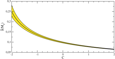
Figure 1: The coupling $\hat{a}(M_{\tau})$ according to Eq. (4) as a function of $C$, and for the ${\overline{\rm MS}}$ input value $\alpha_{s}(M_{\tau})=0.316(10)$. The yellow band corresponds to the $\alpha_{s}$ uncertainty.

2 Application to $\tau$ decays

As a phenomenological application of the $C$-scheme coupling, we focus here on the perturbative expansion of the total $\tau$ hadronic width. The chief observable is the ratio $R_{\tau}$ of the total hadronic branching fraction to the electron branching fraction. It is conventionally decomposed as

$$R_{\tau}\,=\,3\,S_{\rm EW}(|V_{ud}|^{2}+|V_{us}|^{2})\,(1+\delta^{(0)}+\cdots),$$ (8)

where $S_{\rm EW}$ is an electroweak correction and $V_{ud}$, as well as $V_{us}$, CKM matrix elements. Perturbative QCD is encoded in $\delta^{(0)}$ (see Refs. [13, 14] for details) and the ellipsis indicate further small sub-leading corrections. The calculation of $\delta^{(0)}$ is performed from a contour integral of the so called Adler function in the complex energy plane, exploiting analyticity properties, which allows one to avoid the low energy region where perturbative QCD is not valid. In doing so, one must adopt a procedure in order to deal with the renormalization scale. The scale logarithms can be summed either before or after performing the contour integration. The first choice, where the integrals are performed over the running QCD coupling, is called Contour Improved Perturbation Theory (CIPT), while the second, where the coupling is evaluated at a fixed scale and the integrals are performed over the logarithms, is called Fixed Order Perturbation Theory (FOPT).

Analytic results for the coefficients of the Adler function are available up to five loops, or $\alpha_{s}^{4}$ [15]. Here we consider an estimate for the yet unknown fifth order coefficient of the Adler function, namely $c_{51}=283$ [14].

In FOPT, the perturbative series of $\delta^{(0)}(a_{Q})$ in terms of the ${\overline{\rm MS}}$ coupling $a_{Q}$ is given by [15, 14]

$$\delta_{\rm FO}^{(0)}(a_{Q})=a_{Q}+5.202a_{Q}^{2}+26.37a_{Q}^{3}+127.1a_{Q}^{4}+\cdots$$ (9)

In the $C$-scheme coupling $\hat{a}_{Q}$, the expansion for $\delta_{\rm FO}^{(0)}$ is

$$\delta_{\rm FO}^{(0)}(\hat{a}_{Q})=\hat{a}_{Q}+(5.202+2.25C)\,\hat{a}_{Q}^{2}$$

$$\hskip 5.69046pt+(27.68+27.41C+5.063C^{2})\,\hat{a}_{Q}^{3}$$

$$\hskip 5.69046pt+(148.4+235.5C+101.5C^{2}+11.39C^{3})\,\hat{a}_{Q}^{4}$$

$$\hskip 5.69046pt+\cdots$$ (10)

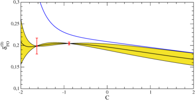
Figure 2: $\delta_{\rm FO}^{(0)}(\hat{a}_{Q})$ of Eq. (2) as a function of $C$. The yellow band arises from either removing or doubling the fifth-order term. In the red dots, the ${\cal O}(\hat{a}^{5})$ vanishes, and ${\cal O}(\hat{a}^{4})$ is taken as the uncertainty. For further explanation, see the text.

In Fig. 2, we display $\delta_{\rm FO}^{(0)}(\hat{a}_{Q})$ as a function of $C$. Assuming $c_{5,1}=283$, the yellow band corresponds to removing or doubling the ${\cal O}(\hat{a}^{5})$ term. A plateau is found for $C\approx-1$. Taking $c_{5,1}=566$ and then doubling the ${\cal O}(\hat{a}^{5})$ results in the blue curve that does not show this stability. Hence, this scenario is disfavoured. In the red dots, which lie at $C=-0.882$ and $C=-1.629$, the ${\cal O}(\hat{a}^{5})$ correction vanishes, and the ${\cal O}(\hat{a}^{4})$ term is taken as the uncertainty, in the spirit of asymptotic series. The point to the right has a substantially smaller error, and yields

$$\delta_{\rm FO}^{(0)}(\hat{a}_{M_{\tau}},C=-0.882)\,=\,0.2047\pm 0.0034\pm 0.0133\,.$$ (11)

The second error covers the uncertainty of $\alpha_{s}(M_{\tau})$. In this case, the direct ${\overline{\rm MS}}$ prediction of Eq. (9) is

$$\delta_{\rm FO}^{(0)}(a_{M_{\tau}})\,=\,0.1991\pm 0.0061\pm 0.0119\,\,\,\,\,({\overline{\rm MS}})\,.$$ (12)

This value is somewhat lower, but within $1\,\sigma$ of the higher-order uncertainty.

In CIPT, contour integrals over the running coupling have to be computed, and hence the result cannot be given in analytical form. The general behaviour is very similar to FOPT, with the exception that now also for $c_{5,1}=566$ a zero of the ${\cal O}(\hat{a}^{5})$ term is found. Employing the value of $C$ which leads to the smaller uncertainty one finds

$$\delta_{\rm CI}^{(0)}(\hat{a}_{M_{\tau}},C=-1.246)\,=\,0.1840\pm 0.0062\pm 0.0084\,.$$ (13)

As has been discussed many times in the past (see e.g. [14]) the CIPT prediction lies substantially below the FOPT results. On the other hand, the parametric $\alpha_{s}$ uncertainty in CIPT turns out to be smaller.

3 Higher-order terms

The behaviour of the series at higher orders is not known exactly. However, realistic models of the Adler function can be constructed in the Borel plane, in which the singularities of the function, namely its renormalon content, is partially known [3]. In Ref. [14] (see also Ref. [16]), models of the Adler function were constructed using the leading renormalons, that largely dominate the higher-order behaviour of the perturbative series. The model is matched to the exactly known coefficients in order to fully reproduce QCD for terms up to $a_{Q}^{4}$. This allows for a complete reconstruction of the series, to arbitrarily high orders in the coupling, and, moreover, one is able to obtain the “true” value of the asymptotic series by means of the Borel sum. In fact, the series is not strictly Borel summable because infra-red renormalons obstruct integration on the positive real axis. The “true” value has, therefore, an inherent ambiguity that stems from the prescription adopted to circumvent the singularities along the contour of integration. This ambiguity is related to non-perturbative physics [3, 14].

Here we perform a preliminary investigation of the behaviour of $\delta^{(0)}$ at higher orders using the $C$-scheme coupling. The Adler function coefficients for terms higher than $a_{Q}^{5}$ are obtained in the ${\overline{\rm MS}}$ scheme from the central model of Ref. [14]. The series can then be translated to the $C$-scheme by means of the perturbative relation between the couplings $a_{Q}$ and $\hat{a}_{Q}$ [2]. Fig. 3 shows four different series that should approach the same Borel summed result, showed as a horizontal band. The four series use as input the coefficients exactly known in QCD with the addition of the estimate $c_{5,1}=283$. One observes that the optimised version of $\delta_{\rm FO}^{(0)}$ (filled circles) approaches the Borel sum of the series faster than the ${\overline{\rm MS}}$ result (empty circles). Of course, because the optimised series has a larger coupling (see Fig. 1) asymptoticity sets in earlier and the divergent character is clearly visible already around the 10th order. The FOPT result with $C=0.7$ shows that smaller couplings do not necessarily lead to a better approximation at lower orders, requiring many more terms to give a good approximation to the Borel summed result. Finally, the optimal CIPT series does not give a good approximation to the Borel summed result (this is also the case in the ${\overline{\rm MS}}$ [14]). Unfortunately, the use of the $C$-scheme coupling does not make the CIPT prediction closer to FOPT. The $C$-scheme FOPT, on the other hand, is in excellent agreement with the central Borel model which suggests that FOPT should be the favoured expansion.

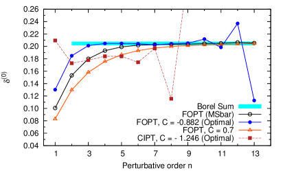
Figure 3: Four series for $\delta^{(0)}$ with higher-order coefficients from the central model of Ref. [14]. In all cases $\alpha_{s}(M_{\tau})=0.316$ which corresponds to the central value of the present world average [17]. The optimised FOPT (filled circles) and CIPT (filled squares) series can be compared with the FOPT ${\overline{\rm MS}}$ results (empty circles) and FOPT for $C=0.7$ (triangles). The shaded band gives the Borel summed result, the “true” value of the series, with its associated ambiguity [2].

References

- [1] W. A. Bardeen, A. J. Buras, D. W. Duke, T. Muta, Deep inelastic scattering beyond the leading order in asymptotically free gauge theories, Phys. Rev. D18 (1978) 3998.
- [2] D. Boito, M. Jamin, R. Miravitllas, Scheme Variations of the QCD Coupling and Hadronic τ Decays, Phys. Rev. Lett. 117 (15) (2016) 152001.
- [3] M. Beneke, Renormalons, Phys. Rept. 317 (1999) 1–142.
- [4] F. J. Dyson, Divergence of perturbation theory in quantum electrodynamics, Phys. Rev. 85 (1952) 631–632.
- [5] S. J. Brodsky, G. P. Lepage, P. B. Mackenzie, On the Elimination of Scale Ambiguities in Perturbative Quantum Chromodynamics, Phys. Rev. D28 (1983) 228.
- [6] S. J. Brodsky, X.-G. Wu, Eliminating the Renormalization Scale Ambiguity for Top-Pair Production Using the Principle of Maximum Conformality, Phys. Rev. Lett. 109 (2012) 042002.
- [7] M. Mojaza, S. J. Brodsky, X.-G. Wu, Systematic All-Orders Method to Eliminate Renormalization-Scale and Scheme Ambiguities in Perturbative QCD, Phys. Rev. Lett. 110 (2013) 192001.
- [8] G. Grunberg, Renormalization Scheme Independent QCD and QED: The Method of Effective Charges, Phys. Rev. D29 (1984) 2315.
- [9] P. A. Baikov, K. G. Chetyrkin, J. H. K hn, Five-Loop Running of the QCD coupling constantarXiv:1606.08659.
- [10] W. Celmaster, R. J. Gonsalves, The renormalization prescription dependence of the QCD coupling constant, Phys. Rev. D20 (1979) 1420.
- [11] L. S. Brown, L. G. Yaffe, C.-X. Zhai, Large order perturbation theory for the electromagnetic current-current correlation function, Phys. Rev. D46 (1992) 4712–4735.
- [12] M. Beneke, PhD Thesis, Munich.
- [13] E. Braaten, S. Narison, A. Pich, QCD analysis of the hadronic width, Nucl. Phys. B373 (1992) 581–612.
- [14] M. Beneke, M. Jamin, and the hadronic width: fixed-order, contour-improved and higher-order perturbation theory, JHEP 09 (2008) 044.
- [15] P. A. Baikov, K. G. Chetyrkin, J. H. Kühn, Order QCD corrections to and decays, Phys. Rev. Lett. 101 (2008) 012002.
- [16] M. Beneke, D. Boito, M. Jamin, Perturbative expansion of tau hadronic spectral function moments and extractions, JHEP 01 (2013) 125.
- [17] C. Patrignani, et al., Review of Particle Physics, Chin. Phys. C40 (10) (2016) 100001.