Noise representation in residuals of LSQR, LSMR, and CRAIG regularization
Abstract
Golub-Kahan iterative bidiagonalization represents the core algorithm in several regularization methods for solving large linear noise-polluted ill-posed problems. We consider a general noise setting and derive explicit relations between (noise contaminated) bidiagonalization vectors and the residuals of bidiagonalization-based regularization methods LSQR, LSMR, and CRAIG. For LSQR and LSMR residuals we prove that the coefficients of the linear combination of the computed bidiagonalization vectors reflect the amount of propagated noise in each of these vectors. For CRAIG the residual is only a multiple of a particular bidiagonalization vector. We show how its size indicates the regularization effect in each iteration by expressing the CRAIG solution as the exact solution to a modified compatible problem. Validity of the results for larger two-dimensional problems and influence of the loss of orthogonality is also discussed.
Keywords
ill-posed problems, regularization, Golub-Kahan iterative bidiagonalization, LSQR, LSMR, CRAIG
AMS classification
15A29, 65F10, 65F22
1 Introduction
In this paper we consider ill-posed linear algebraic problems of the form
| (1) |
where the matrix represents a discretized smoothing operator with the singular values decaying gradually to zero without a noticeable gap. We assume that multiplication of a vector by or results in smoothing which reduces the relative size of the high-frequency components of . The operator and the vector are supposed to be known. The vector represents errors, such as noise, that affect the exact data. Problems of this kind are commonly referred to as linear discrete ill-posed problems or linear inverse problems and arise in a variety of applications [1, 2]. Since is ill-conditioned, the presence of noise makes the naive solution
| (2) |
where denotes the Moore-Penrose pseudoinverse, meaningless. Therefore, to find an acceptable numerical approximation to , it is necessary to use regularization methods.
Various techniques to regularize the linear inverse problem (1) have been developed. For large-scale problems, iterative regularization is a good alternative to direct regularization methods. When an iterative method is used, regularization is achieved by early termination of the process, before noise starts to dominate the approximate solution [1]. Many iterative regularization methods such as LSQR [3, 4, 5, 6], CRAIG [7, 8], LSMR [9], and CRAIG-MR/MRNE [10, 11] involve the Golub-Kahan iterative bidiagonalization [12]. Combination with an additional inner regularization (typically with a spectral filtering method) gives so-called hybrid regularization; see, for example, [4, 13, 14, 15]. Various approaches for choosing the stopping criterion, playing here the role of the regularization parameter, are based on comparing the properties of the actual residual to an a priori known property of noise, such as the noise level in the Morozov’s discrepancy principle [16], or the noise distribution in the cumulative residual periodogram method [17, 18, 19]. Thus understanding how noise translates to the residuals during the iterative process is of great interest.
The aim of this paper is, using the analysis of the propagation of noise in the left bidiagonalization vectors provided in [20], to study the relation between residuals of bidiagonalization-based methods and the noise vector . Whereas in [20], white noise was assumed, here we have no particular assumptions on the distribution of noise. We only assume the amount of noise is large enough to make the noise propagation visible through the smoothing by in construction of the bidiagonalization vectors. This is often the case in ill-posed problems, as we illustrate on one-dimensional (1D) as well as significantly noise contaminated two-dimensional (2D) benchmarks. We prove that LSQR and LSMR residuals are given by a linear combination of the bidiagonalization vectors with the coefficients related to the amount of propagated noise in the corresponding vector. For CRAIG, the residual is only a multiple of a particular bidiagonalization vector. This allows us to prove that an approximate solution obtained in a given iteration by CRAIG applied to (1) coincides with an exact solution of the (compatible) modified problem
| (3) |
where is a noise vector estimate constructed from the currently computed bidiagonalization vectors. These results contribute to understanding of regularization properties of the considered methods and should be considered when devising reliable stopping criteria.
Note that since LSQR is mathematically equivalent to CGLS and CGNR, CRAIG is mathematically equivalent to CGNE and CGME [21], and LSMR is mathematically equivalent to CRLS [9], then in exact arithmetic, the analysis applies also to these methods.
The paper is organized as follows. In Section 2, after a recollection of the previous results, we study the propagation of various types of noise and the influence of the loss of orthogonality on this phenomenon. Section 3 investigates the residuals of selected methods with respect to the noise contamination in the left bidiagonalization vectors and compares their properties. Section 4 discusses validity of obtained results for larger 2D problems. Section 5 concludes the paper.
Unless specified otherwise, we assume exact arithmetic and the presented experiments are performed with full double reorthogonalization in the bidiagonalization process. Throughout the paper, denotes the standard Euclidean norm of the vector , vector denotes the -th column of the identity matrix. By , we denote the set of polynomials of degree less or equal to . The noise level is denoted by . By Poisson noise, we understand , i.e., the right-hand side is a Poisson random with the Poisson parameter . The test problems were adopted from the Regularization tools [22]. For simplicity of exposition, we assume the initial approximation throughout the paper. Generalization to is straightforward.
2 Properties of the Golub-Kahan iterative bidiagonalization
2.1 Basic relations
Given the initial vectors , , where , the Golub-Kahan iterative bidiagonalization [12] computes, for ,
| (4) | ||||||
| (5) |
until or , or until . Vectors , and , form orthonormal bases of the Krylov subspaces and , respectively. In the rest of the paper, we assume that the bidiagonalization process does not terminate before the iteration , i.e., ,
Denoting and
| (6) |
we can write the matrix version of the bidiagonalization as
| (7) |
The two corresponding Lanczos three-term recurrences
| (8) |
allow us to describe the bidiagonalization vectors and in terms of the Lanczos polynomials as
| (9) |
see [3, 4, 23, 24, 25]. From (9) we have that
| (10) |
giving
| (11) |
The first component on the right-hand side of (11) can be rewritten as
| (12) |
for some . Since has the smoothing property, then is smooth for . Thus is a sum of a low-frequency vector and the scaled noise vector ,
| (13) |
Note that this splitting corresponds to the low-frequency part and propagated (non-smoothed) noise part only when . For large s, there is a considerable cancellation between and , the splitting (13) still holds but it does not correspond to our intuition of an underlying smooth vector and some added scaled noise. Thus we restrict ourselves to smaller values of .
It has been shown in [20] that whereas for (the scaled right-hand side) the noise part in (13) is small compared to the true data, for larger , due to the smoothing property of the matrix and the orthogonality between the vectors , the noise part becomes more significant. The noise scaling factor determining the relative amplification of the non-smoothed part of noise corresponds to the constant term of the Lanczos polynomial
| (14) |
called the amplification factor.111Note that in [20] a different notation was used. The Lanczos polynomial was scaled by so that . The vector was split into . In our notation, , and . Its behavior for problems with white noise was studied in [20] and the analysis concludes that its size increases with until the noise revealing iteration , where the vector is dominated by the non-smoothed part of noise. Then the amplification factor increases at least for one iteration. The noise revealing iteration can be defined as Note that there is no analogy for the right bidiagonalization vectors, since all vectors are smoothed and the factor on average grows till late iterations. A recursive relation for , obtained directly from (5) has the form
| (15) | ||||
| (16) |
2.2 Behavior of the noise amplification factor
Influence of the noise frequency characteristics
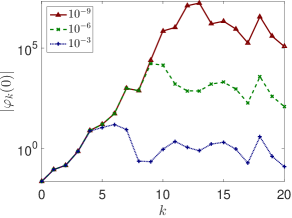
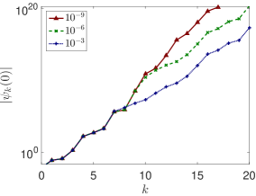
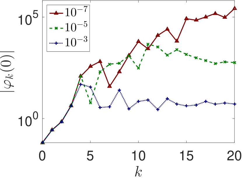
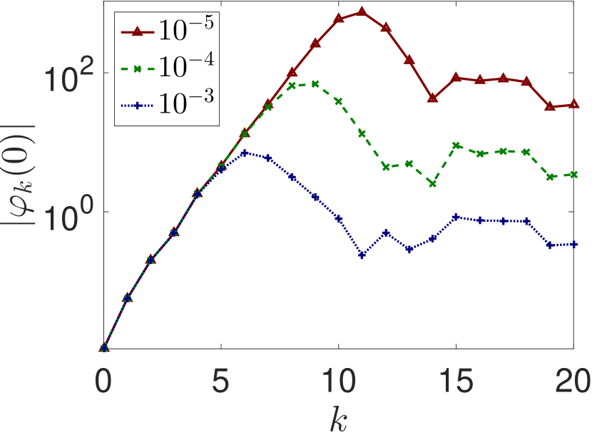
The phenomenon of noise amplification is demonstrated on the problems from [26, 22]. Figures 1(b) and 1(c) show the absolute terms of the Lanczos polynomials and for the problem shaw polluted with white noise of various noise levels. For example, for the noise level , the maximum of is achieved for , which corresponds to the observation that the vector in Figure 1(a) is the most dominated by propagated noise. Obviously, the noise revealing iteration increases with decreasing noise level. The amplification factors exhibit similar behavior before the first decrease. However, the behavior of can be more complicated. In Figure 2(a) for phillips, the sizes of the amplification factors oscillate as a consequence of the oscillations in the sizes of the spectral components of in the left singular subspaces of . Thus there is a partial reduction of the noise component, which influences the subsequent iterations, even before the noise revealing iteration.

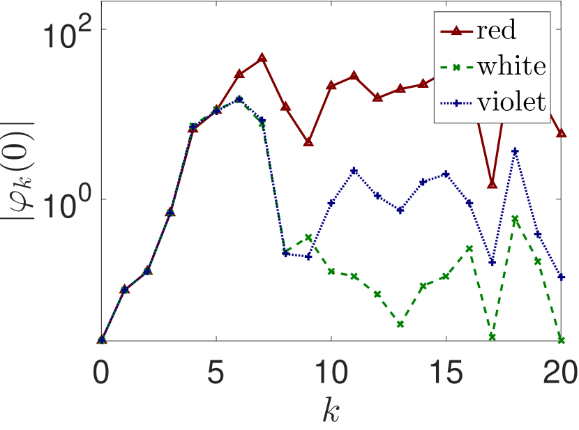
Even though [20] assumed white noise, noise amplification can be observed also for other noise settings and the formulas (9)-(16) still hold. However, for high-frequency noise, there is smaller cancellation between the low-frequency component and the noise part in (13). Therefore, in the orthogonalization steps succeeding the noise revealing iteration , the noise part is projected out more significantly. For low-frequency noise, on the other side, this smoothing is less significant, which results in smaller drop of (14) after . This is illustrated in Figure 2(b) on the problem shaw polluted by red (low-frequency), white, and violet (high-frequency) noise of the same noise level. For spectral characteristics of these types of noise see Figure 3.
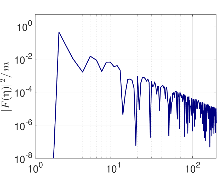
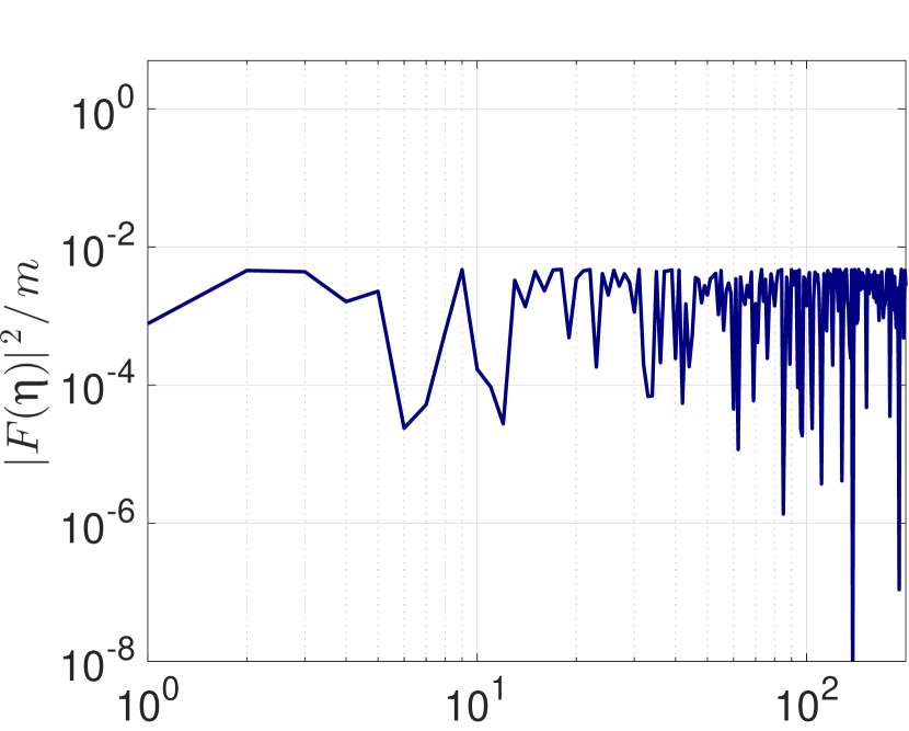
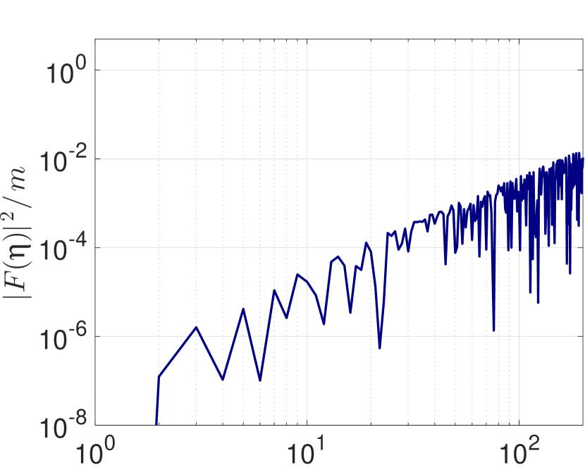
Figure 2(c) shows the amplification factor for various levels of Poisson noise.
Influence of the loss of orthogonality
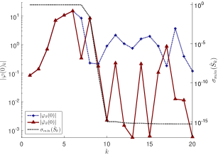
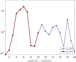
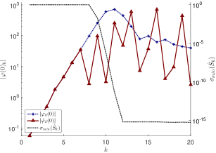
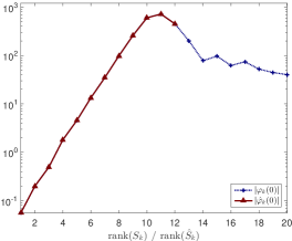
First note that the splitting (13) remains valid even if are not exactly orthonormal Lanczos polynomials, since the propagated noise can be still tracked using the absolute term of the corresponding (computed) polynomial. Nevertheless, it is clear that the loss of orthogonality among the left bidiagonalization vectors in finite precision arithmetic influences the behavior of the amplification factor , i.e. the propagation of noise. In the following, we denote all quantities computed without reorthogonalization by hat. Loss of orthogonality can be detected, e.g., by tracking the size of the smallest singular value of the matrix of the computed left bidiagonalization vectors. In Figure 4 (left) for the problem shaw and gravity we see that when drops below one detecting the loss of orthogonality among its columns, the size of the amplification factor starts to oscillate. However, except of the delay, the larger values of still match those of . If we plot against the rank of instead of , the sizes of the two amplification factors become very similar. In our experiments, the rank of was computed as rank(S(:,1:k),1e-1) in MATLAB, i.e., singular values of at least ten times smaller than they would be for orthonormal columns were considered zero. A similar shifting strategy was proposed in [28, chap. 3] for the convergence curves of the conjugate gradient method. Note that the choice of the tolerance can be problem dependent. Further study of this phenomenon is beyond the scope of this paper, but we can conclude that except of the delay the noise revealing phenomenon is in finite precision computations present.
3 Noise in the residuals of iterative methods
CRAIG [7], LSQR [3], and LSMR [9] represent three methods based on the Golub-Kahan iterative bidiagonalization. At the -th step, they search for the approximation of the solution in the subspace generated by vectors , i.e.,
| (17) |
The corresponding residual has the form
| (18) |
CRAIG minimizes the distance of from the naive solution yielding
| (19) |
LSQR minimizes the norm of the residual yielding
| (20) |
LSMR minimizes the norm of giving
| (21) |
These methods are mathematically equivalent to Krylov subspace methods based on the Lanczos tridiagonalization (particularly Lanczos for linear systems and MINRES) applied to particular normal equations. The relations useful in the following derivations are summarized in Table 1.
| method/equation | |||
|---|---|---|---|
| Lanczos method | LSQR | CRAIG | — |
| MINRES | LSMR | LSQR | CRAIG |
Since Lanczos method is a Galerkin (residual orthogonalization) method, we immediately see that
| (22) | ||||
| (23) |
Using the relation between the Galerkin an the residual minimization method, see[21, sec. 6.5.7], we obtain,
| (24) | ||||
| (25) |
Note that these equations hold, up to a small perturbation, also in finite precision computations. See [29] for more details.
In the rest of this section, we investigate the residuals of each particular method. We focus on in which sense the residuals approximate the noise vector. We discuss particularly the case when noise contaminates the bidiagonalization vectors fast and thus the noise revealing iteration is well defined. More general discussion follows in Section 4.
3.1 CRAIG residuals
The following result relates approximate solution obtained by CRAIG for (1) to the solution of the problem with the same matrix and a modified right-hand side.
Proposition 1.
Proof.
First note that we only need to show that , . From (23) and (9) it follows that there exist , such that
| (28) |
Let us now determine the constant . From (18) and (9), we have that
| (29) |
Combining these two equations, we obtain
| (30) |
Substituting to (30) back from (9), we immediately have (26). Since , (27) is a direct consequence of (26). ∎∎
Although the relation (26) is valid for any problem of the form (1), it has a particularly interesting interpretation for inverse problems with a smoothing operator . Suppose we neglect the low-frequency part in (13) and estimate the unknown noise from the left bidiagonalization vector as
| (31) |
Subtracting from in (1), we obtain exactly the modified problem (26). Thus Proposition 1 in fact states that in each iteration , represents the exact solution of the problem (3) with noise being approximated by a particular re-scaled left bidiagonalization vector.
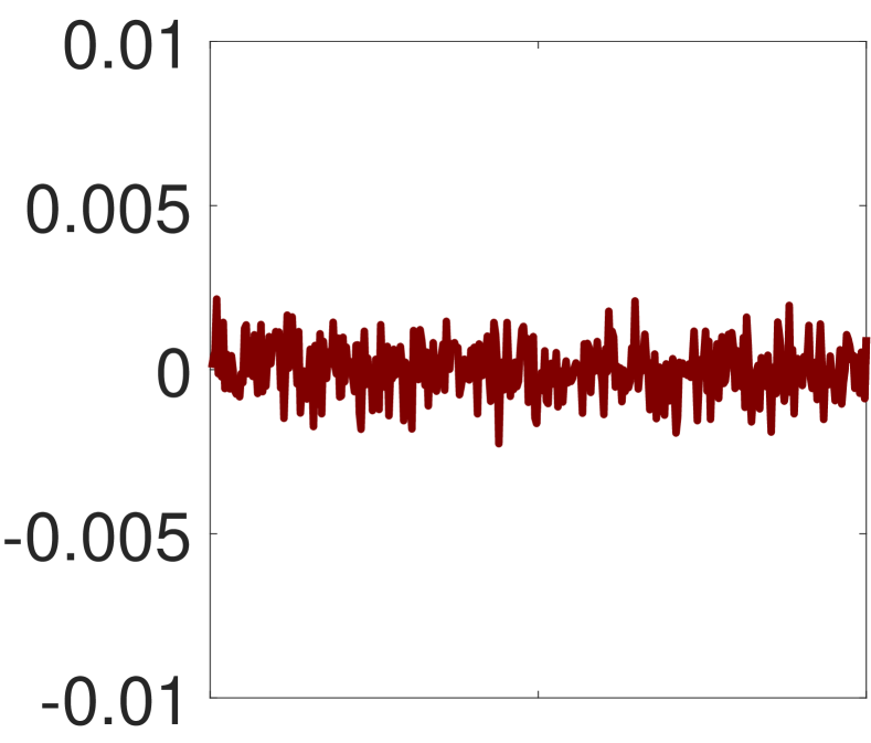
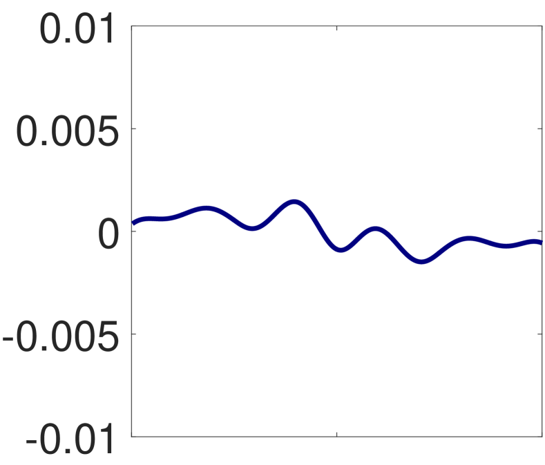
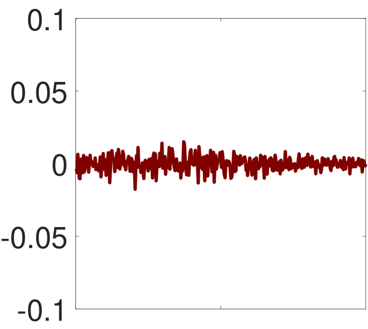
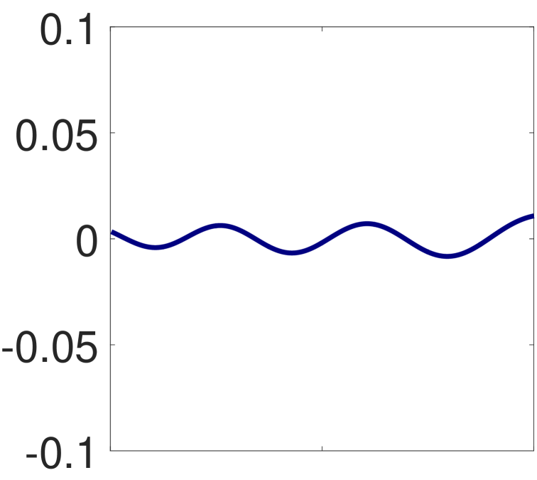
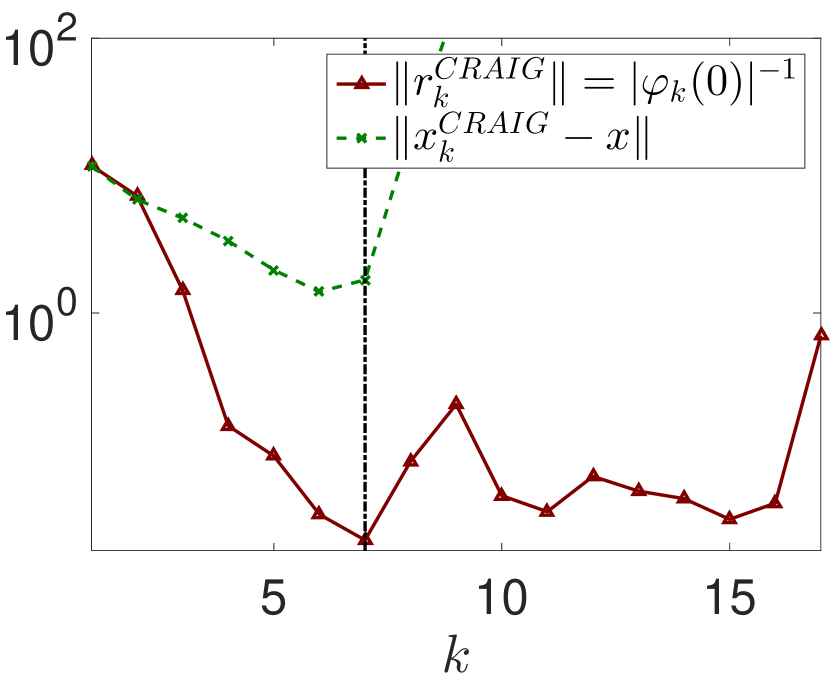
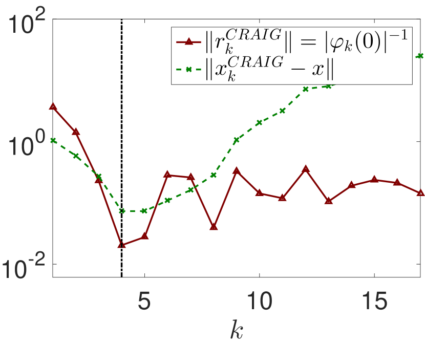
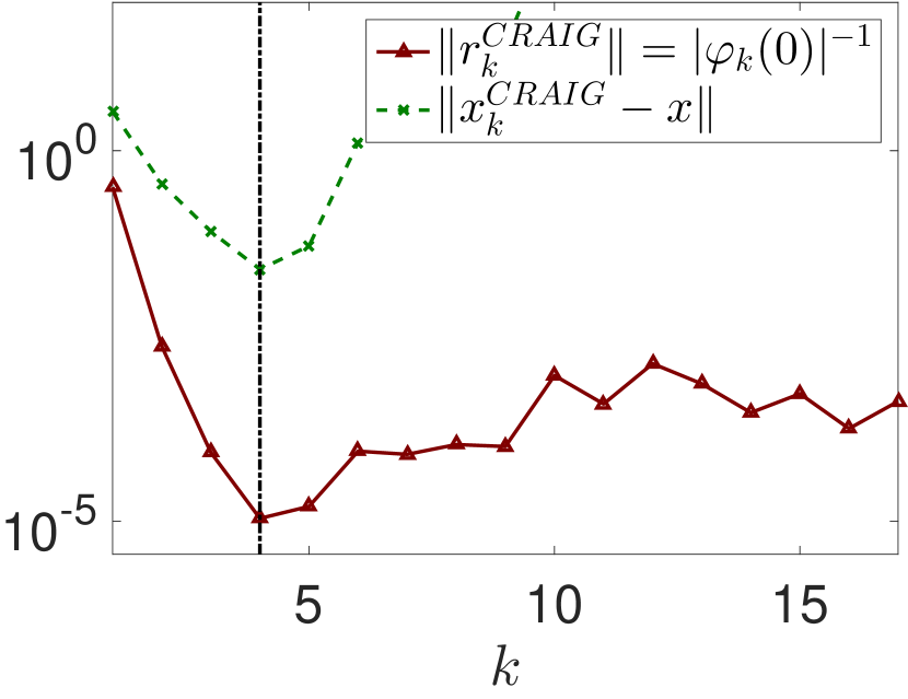
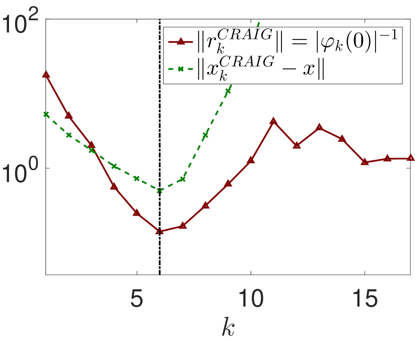
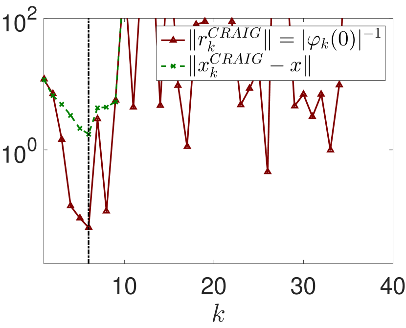
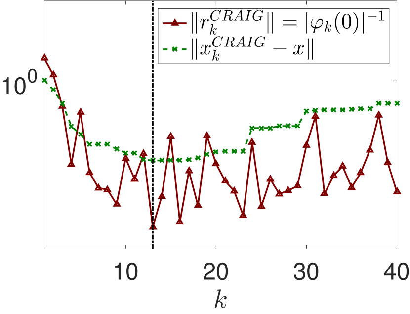
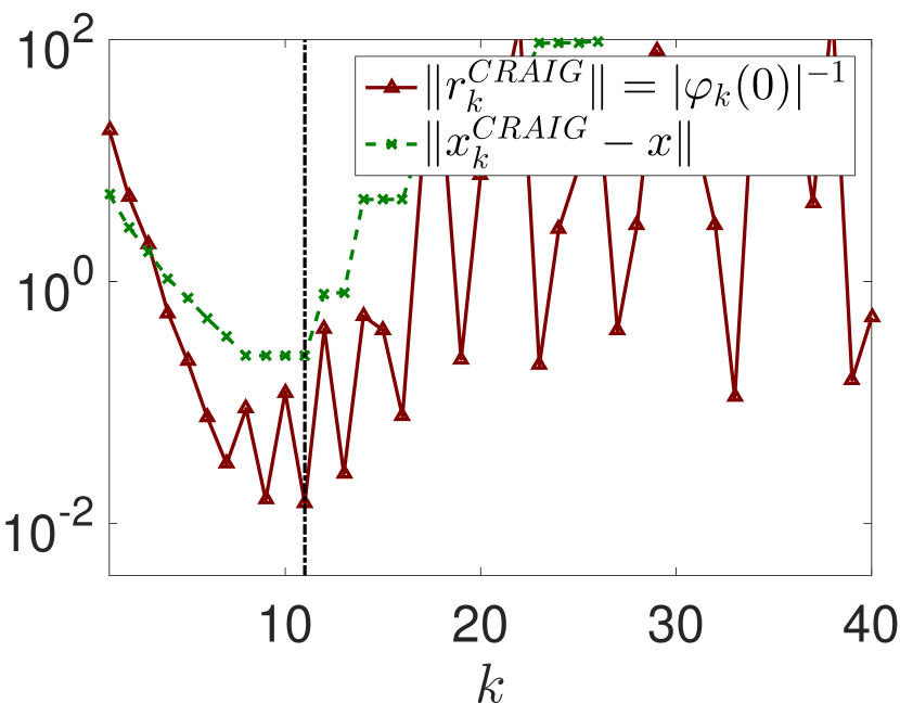
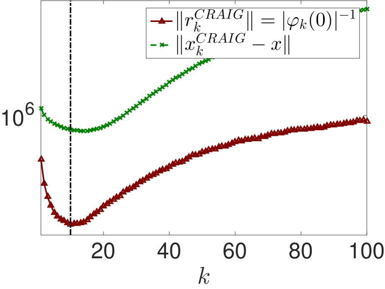
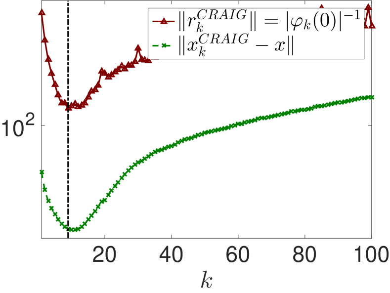
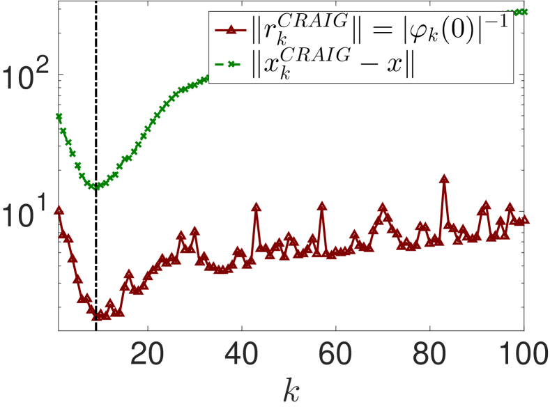
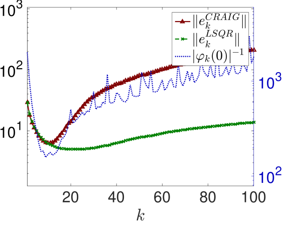
The norm of the CRAIG residual is inversely proportional to the amount of noise propagated to the currently computed left bidiagonalization vector. It reaches its minimum exactly in the noise revealing iteration , which corresponds to the iteration with (31) being the best approximation of the unknown noise vector. The actual noise vector and the difference for obtained from are compared in Figure 5; see also [30]. We see that in iteration , the troublesome high-frequency part of noise is perfectly removed. The remaining perturbation only contains smoothed, i.e., low-frequency part of the original noise vector. The match in (27) remains valid, up to a small perturbation, also in finite precision computations, since the noise propagation is preserved, see Section 2.2
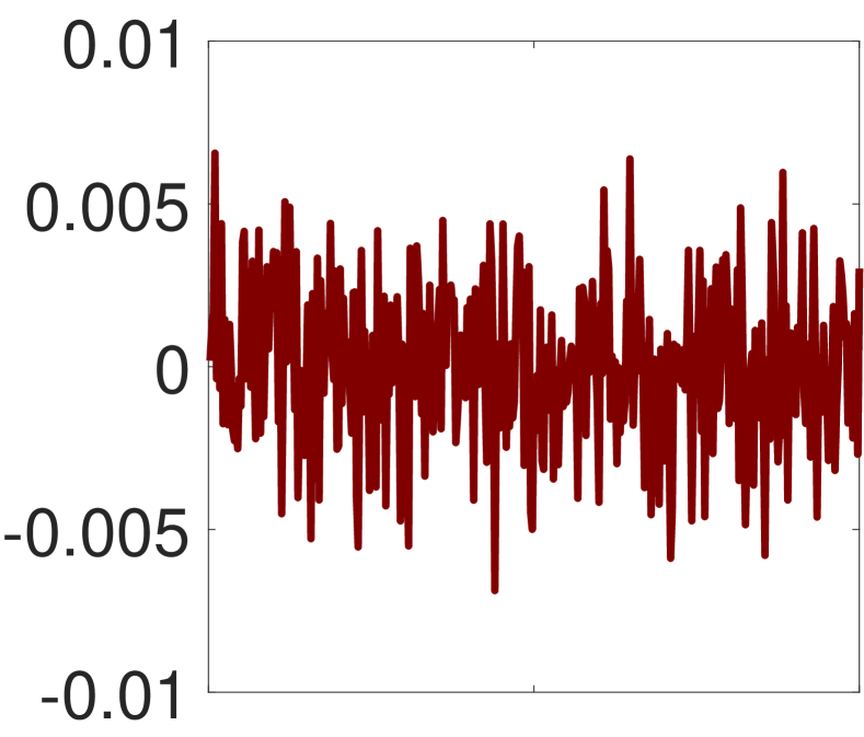
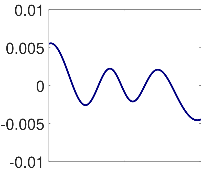
,
white noise
,
white noise
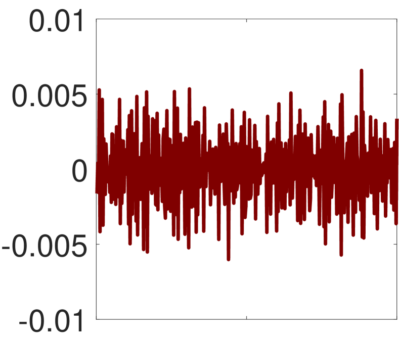
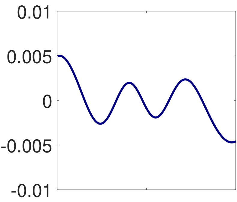
,
violet noise
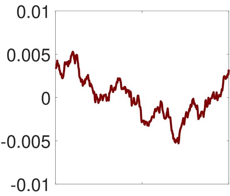
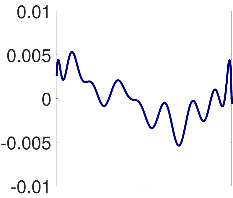
,
red noise
,
Poisson noise
Note that due to different frequency characteristic of and for small , there is a relatively small cancellation between them and
| (32) |
This gives
| (33) |
supporting our expectation that the size of the remaining perturbation depends on how closely the inverse amplification factor approaches .
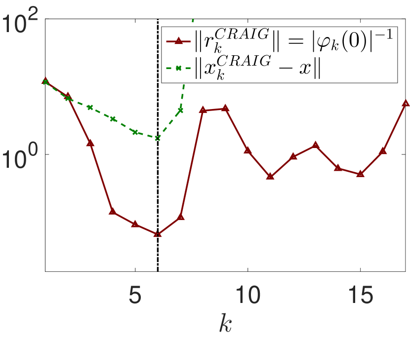
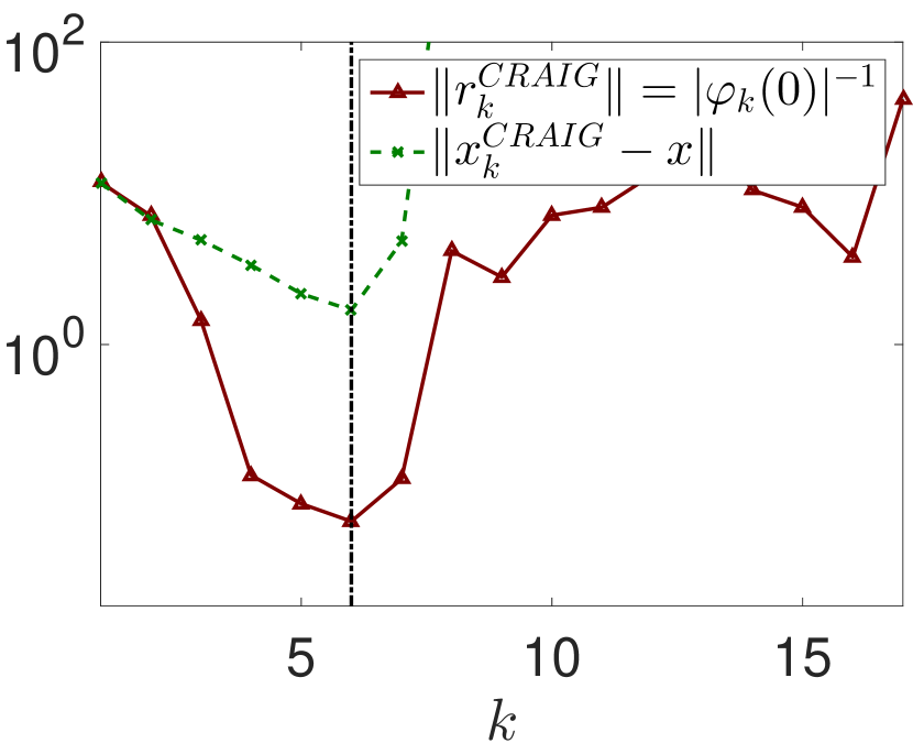
We may also conclude that for ill-posed problems with a smoothing operator , the minimal error is reached approximately at the iteration with the maximal noise revealing, i.e., with the minimal residual. This is confirmed by numerical experiments in Figure 6 comparing with for various test problems and noise characteristics, both with and without reorthogonalization.
, white noise
, Poisson
, white noise
, white noise
, Poisson
3.2 LSQR residuals
Whereas for CRAIG, the residual is just a scaled left bidiagonalization vector, for LSQR it is a linear combination of all previously computed left bidiagonalization vectors. Indeed,
| (34) |
see (18). The entries of the residual of the projected problem
| (35) |
see (20), represent the coefficients of the linear combination in (34). The following proposition shows the relation between the coefficients and the amplification factor .
Proposition 2.
Proof.
In other words, Proposition 2 says that the coefficients of the linear combination (34) follow the behavior of the amplification factor in the sense that representation of a particular left bidiagonalization vector in the residual , , is proportional to the amount of propagated non-smoothed part of noise in this vector.
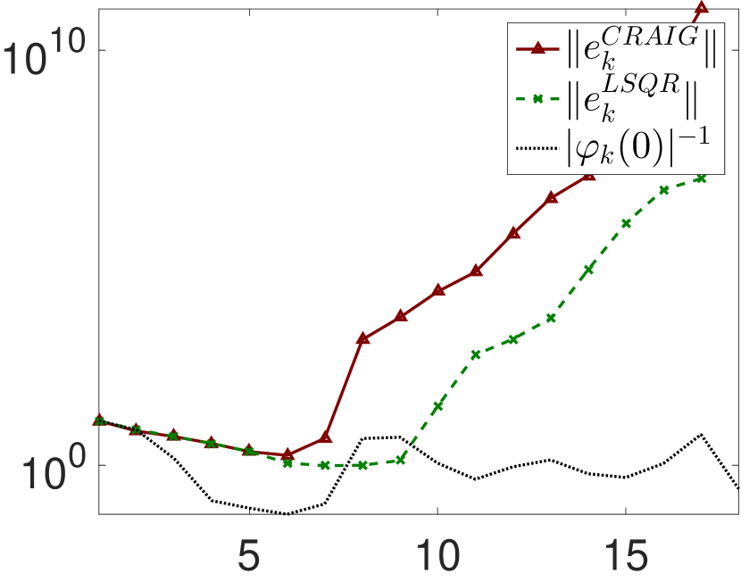
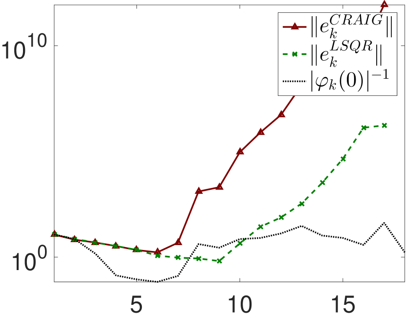
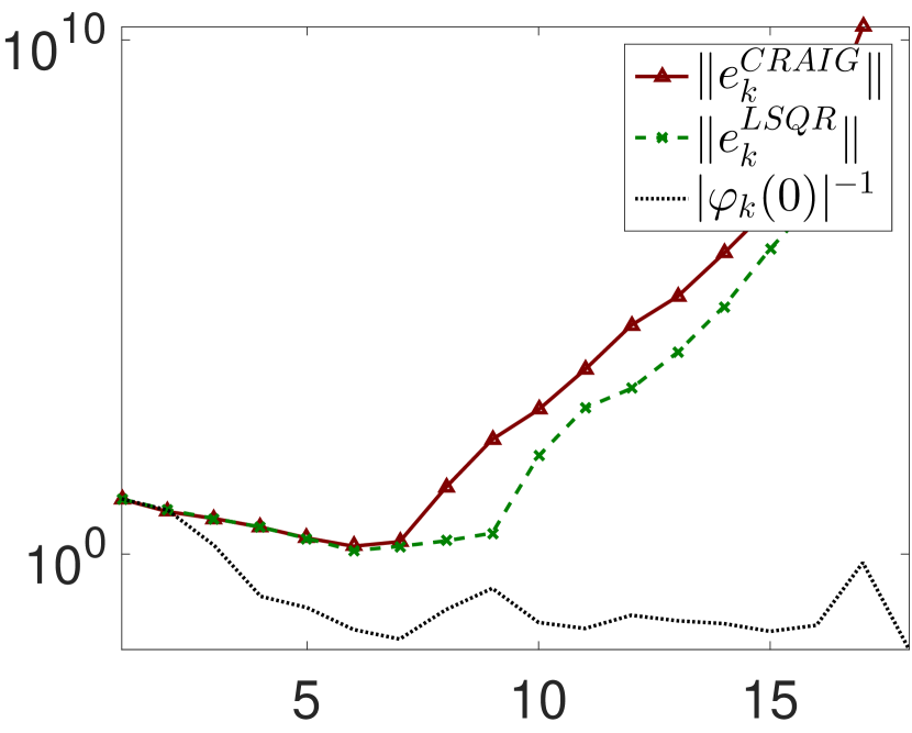
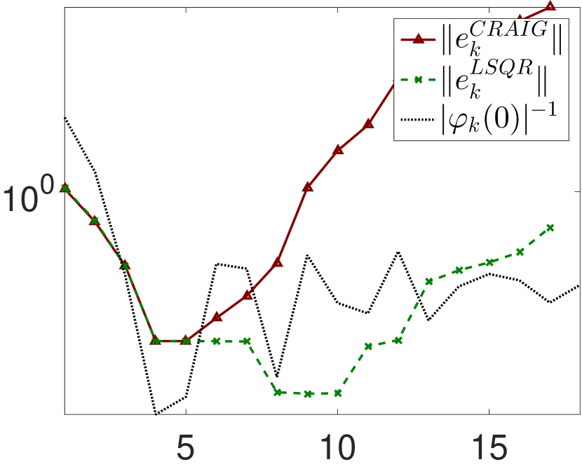
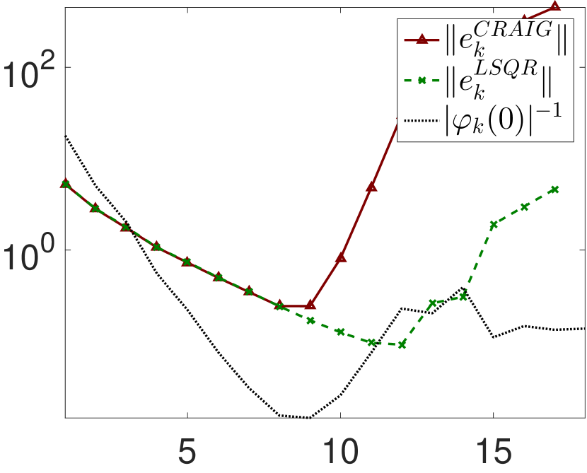
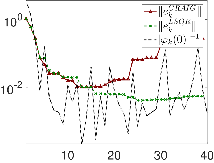
Relation (36) also suggests that the norm-minimizing process (LSQR) and the corresponding Galerkin process (CRAIG) provide similar solutions whenever
| (44) |
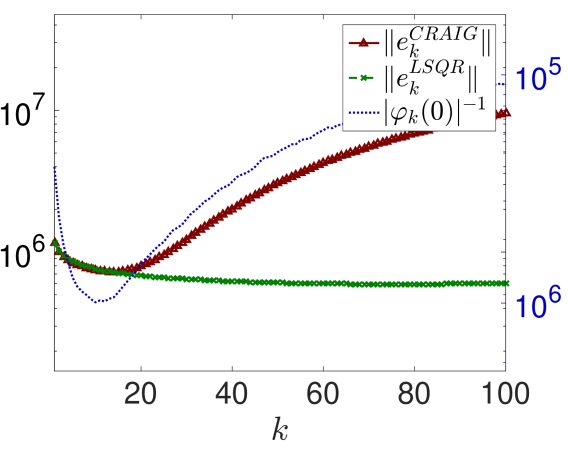
i.e., whenever the noise revealing in the last left bidiagonalization vector is much more significant than in all previous left bidiagonalization vectors , i.e., typically before we reach the noise revealing iteration. This is confirmed numerically in Figure 7, comparing the semiconvergence curves of CRAIG and LSQR.
, white noise
, white noise
3.3 LSMR residuals
Before we investigate the residual of LSMR with respect to the basis , we should understand how it is related to the residual of LSQR. It follows from Table 1 that the relation between and is analogous to the relation between and . Using Proposition 1 and 2, with substituted by and substituted by , we obtain
| (45) |
and
| (46) |
Since
| (47) |
we obtain that
| (53) |
This equality however does not provide the desired relationship between the residuals themselves and the left bidiagonalization vectors . This is given in the following proposition.
Proposition 3.
Proof.
From (53) it follows that
| (55) |
where is an upper triangular matrix with entries
| (56) |
Thus
| (57) |
where extracts the upper triangular part of the matrix. Multiplying out, we obtain
| (58) |
∎∎
Here the sizes of coefficients in need careful discussion. From (14) and (16) it follows that the absolute terms of the Lanczos polynomials and have the same sign. Thus we have
| (59) |
and therefore the sum
| (60) |
decreases when increases. Furthermore, it was shown in [20, sec. 3.2] that for
| (61) |
Thus (14) yields
However, since on average increases rapidly with (see Section 2.2), the sizes of the entries of in (58) generally increase with before . After reaches the noise revealing iteration , decreases at least for one but typically for more subsequent iterations; see Section 2.2. Multiplication by the decreasing (60) causes that the size of the entries in (58) can be expected to decrease after .
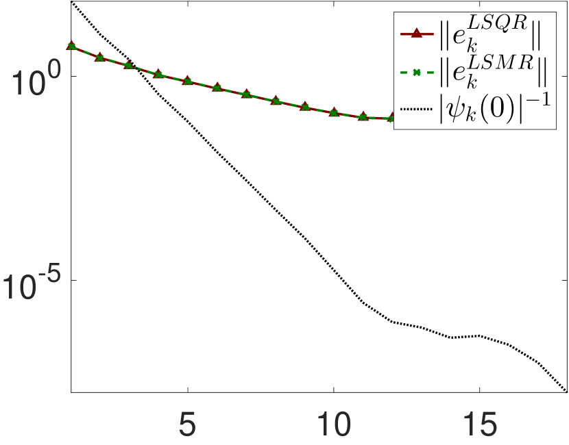
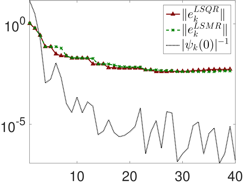
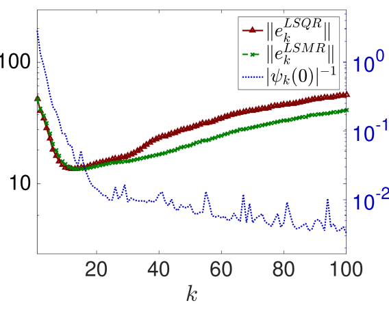
From the previous we conclude that the behavior of the entries of resembles the behavior of , i.e., the size of a particular entry is proportional to the amount of propagated noise in the corresponding bidiagonalization vector, similarly as in the LSQR method. Figure 8 compares the entries of with appropriately re-scaled amplification factor on the problem shaw with white noise. We see that the difference is negligible an therefore the residuals for LSQR and LSMR resemble. In early iterations, the resemblance of the residuals indicates resemblance of the solutions since the remaining perturbation only contains low frequencies, which are not amplified by .
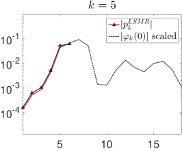
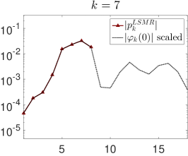
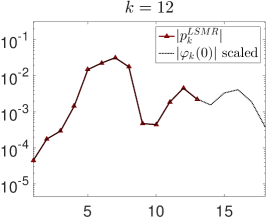
Note also that since grows rapidly on average, see Figure 1(c) in Section 2.2, we may expect
| (62) |
Therefore resembles giving another explanation why LSMR and LSQR behave similarly for inverse problems with a smoothing operator , see Figure 9 for a comparison on several test problems.
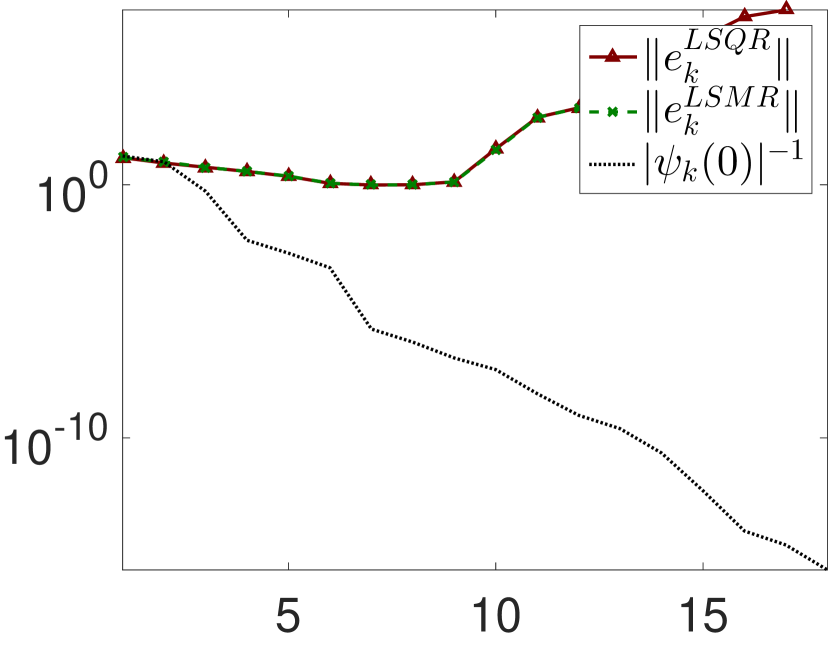
, white noise
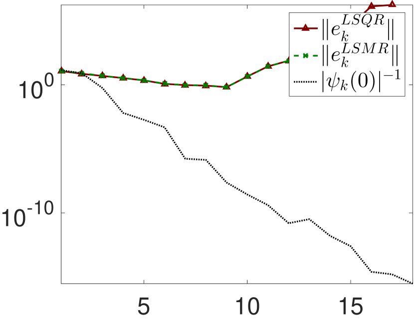
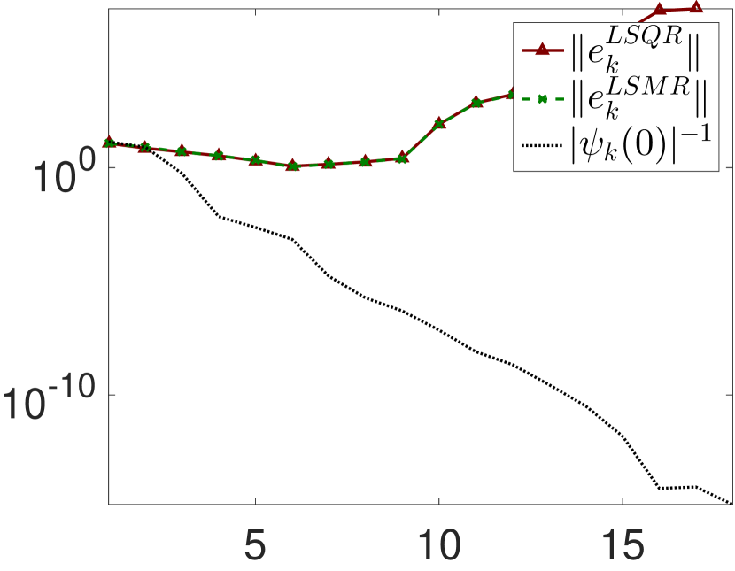
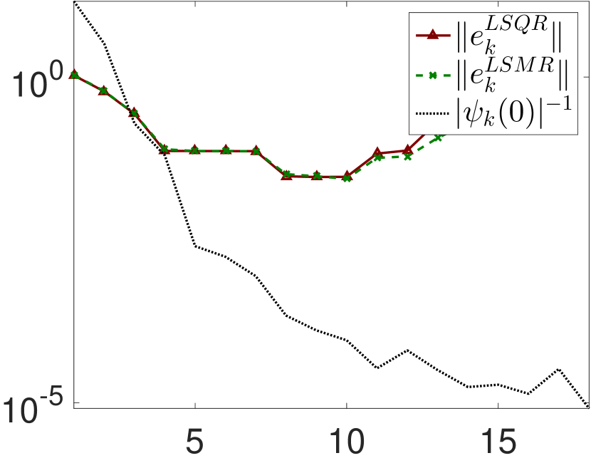
, white noise
Figure 10 illustrates the match between the noise vector and residual of CRAIG, LSQR and LSMR method. We see that while CRAIG residual resembles noise only in the noise revealing iteration, LSQR and LSMR are less sensitive to the particular number of iterations as the residuals are combinations of bidiagonalization vectors with appropriate coefficients. Moreover, the best match in LSQR and LSMR method overcomes the best match in CRAIG. This is caused by the fact that the remaining low-frequency part is efficiently suppressed by the linear combination.


4 Numerical experiments for 2D problems
In this section we discuss validity of the conclusions made above for larger 2D inverse problems, where the smoothing property of (revealing itself in the decay of singular values) is typically less significant. Consequently, noise propagation in the bidiagonalization process may be more complicated; see also [36]. However, we illustrate that essential aspects of the behavior described in previous sections are still present. Note that all experiments in this section are computed without reorthogonalization. We consider the following 2D benchmarks:
-
Medical tomography problem — a simplified 2D model of X-ray medical tomography adopted from [31], function paralleltomo(256,0:179,362). The data is represented the -by- discretization of the Shepp–Logan phantom projected in angles by parallel rays, resulting in a linear algebraic problem with . We use Poisson-type additive noise generated as follows (see [34, chap. 2.6] and [35]) to simulate physically realistic noise:
A = paralleltomo(N,theta)/N; % forward model t = exp(-A*x); % transmission probabilities c = poissrnd(t*N0); % photon counts eta = -log(c/N0); % noisy measurements
where denotes the mean number of photons, resulting in the noise level . We refer to this test problem as paralleltomo.
-
Seismic tomography problem — a simplified 2D model of seismic tomography adopted from [31], function seismictomo(100,100,200). The data is represented by a -by- discretization of a vertical domain intersecting two tectonic plates with sources located on its right boundary and receivers (seismographs), resulting in a linear algebraic problem with . The right-hand side is polluted with additive white noise with . We refer to this test problem as seismictomo.
-
Image deblurring problem — an image deblurring problem with spatially variant blur adopted from [32, 33], data VariantGaussianBlur1. The data is represented by a monochrome microscopic -by- image of a grain blurred by spatially variant Guassian blur (with different point-spread functions), resulting in a linear algebraic problem with . The right-hand side is polluted with additive white noise with . We refer to this test problem as vargaussianblur.
Figure 11 shows the absolute terms of the Lanczos polynomials and . We can identify the two phases of the behavior of – average growth and average decay. However, the transition does not take place in one particular (noise revealing) iteration, but rather in a few subsequent steps, which we refer to as the noise revealing phase of the bidiagonalization process. The size of grows on average till late iterations, however, we often observe here that the speed of this growth slows down after the noise revealing phase. In conclusion, both curves and can be flatter than for 1D problem considered in previous sections. This can be further pronounced for problems with low noise levels.
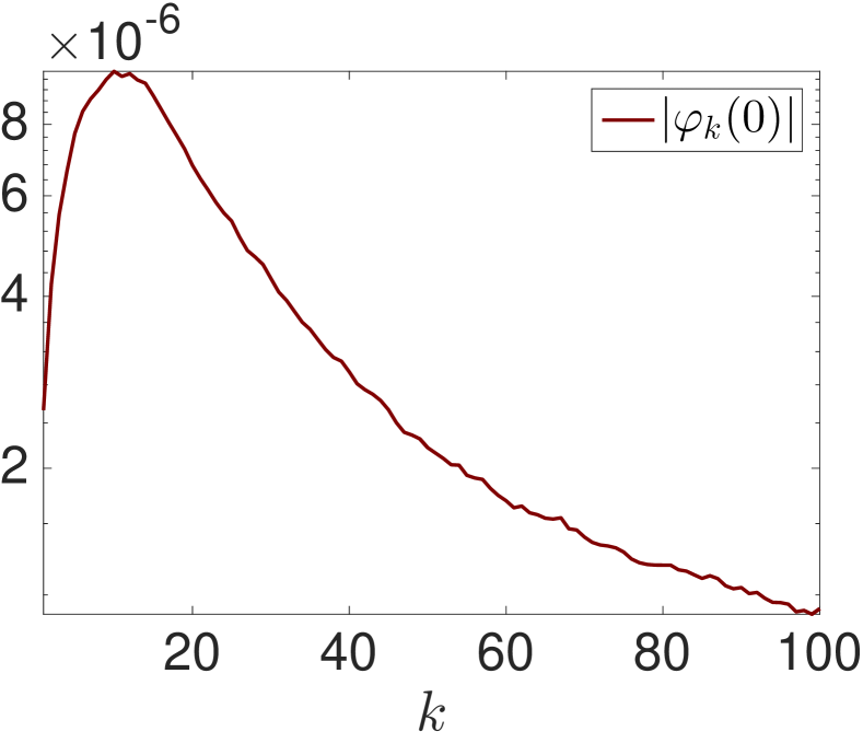
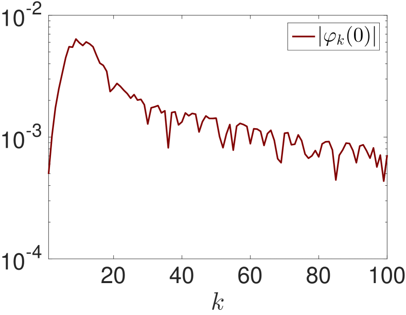
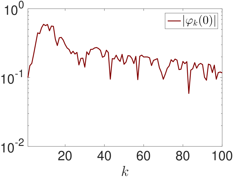
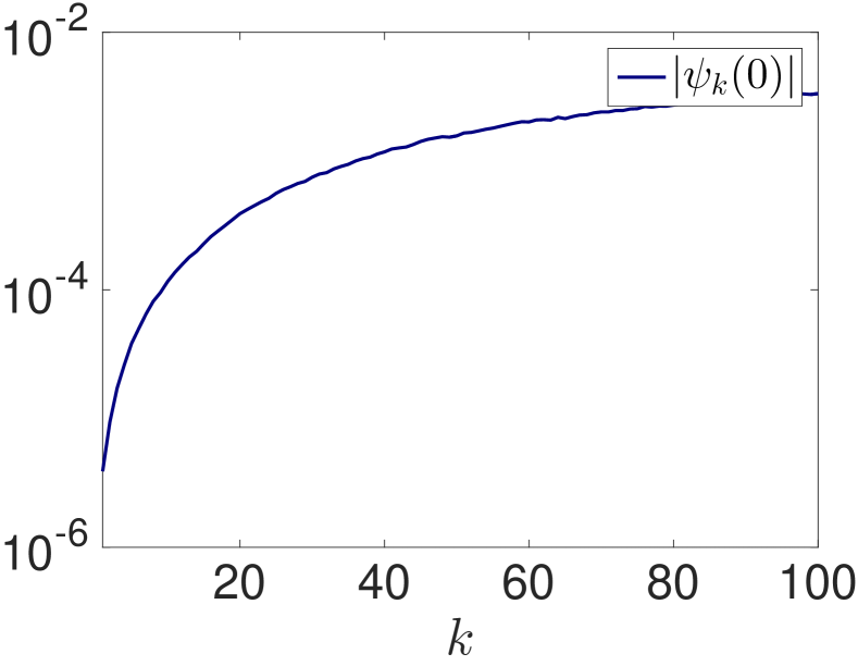
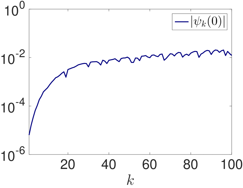
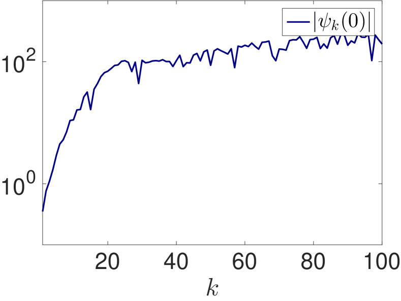
Figure 12 shows several (appropriately reshaped) left bidiagonalization vectors and their cumulative periodograms for the problem seismictomo. Even though it is hard to make clear conclusions based on the vectors themselves, we see that the periodogram for is flatter than the periodograms for smaller or larger values of , meaning that resembles most white noise. This corresponds to Figure 11(b) showing that belongs to the noise revealing phase of the bidiagonalization process. Note that similar flatter periodograms can be obtained for other few vectors belonging to this phase.


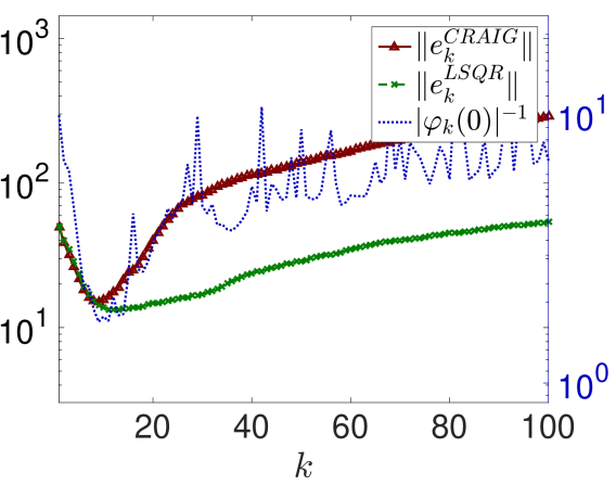
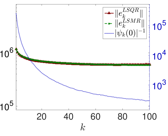
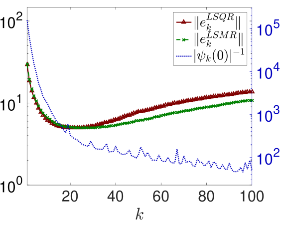
The absence of one particular noise revealing vector makes the direct comparison between and the exact noise vector irrelevant here. However, Propositions 1–3 remain valid and the overall behavior of the terms and is as expected, allowing comparing the bidiagonalization-based methods. Figure 13 gives comparisons of CRAIG, LSQR and LSMR for all considered 2D test problems, analogous to Figure 6, 7, and 9. The first row of Figure 13 shows that the CRAIG error is minimized approximately in the noise revealing phase, i.e., when the residual is minimal, see Section 3.1. The minimum is emphasized by the vertical line.
The second row of Figure 13 compares the errors of CRAIG and LSQR. According to the derivations in Section 3.2, the curves are similar before the noise revealing phase, after which they separate with CRAIG diverging more quickly. Note that the size of the inverted amplification factor is included to illustrate the noise revealing phase and has different scaling (specified on the right).
The third row of Figure 13 shows the errors of LSQR and LSMR with the underlying size of the inverted factor (scaling specified on the right). The errors behave similarly as long as decays rapidly, see Section 3.3. The LSMR solution is slightly less sensitive to the particular choice of the number of bidiagonalization iterations , which is a well know property [9].
5 Conclusion
We proved that approximating the solution of an inverse problem by the th iterate of CRAIG is mathematically equivalent to solving consistent linear algebraic problem with the same matrix and a right-hand side, where a particular (typically high-frequency) part of noise is removed. Using the analysis of noise propagation, we showed that the size of the CRAIG residual is given by the inverted noise amplification factor, which explains why optimal regularization properties are often obtained when the minimal residual is reached. For LSQR and LSMR, the residual is a linear combination of the left bidiagonalization vectors. The representation of these vectors in the residuals is determined by the amplification factor, in particular, left bidiagonalization vectors with larger amount of propagated noise are on average represented with a larger coefficient in both methods. These results were used in 1D problems to compare the methods in terms of matching between the residuals and the unknown noise vector. For large 2D (or 3D) problems the direct comparison of the vectors may not be possible, since noise reveals itself in a few subsequent bidiagonalization vectors (noise revealing phase of bidiagonalization) instead of in one particular iteration. However, the conclusions on the methods themselves remain generally valid. Presented results contribute to understanding of the behavior of the methods when solving noise-contaminated inverse problems.
Acknowledgment
Research supported in part by the Grant Agency of the Czech Republic under the grant 17-04150J. Work of the first and the second author supported in part by Charles University, project GAUK 196216. The authors are grateful to the anonymous referee for useful suggestions and comments that improved the presentation of the paper.
References
References
-
[1]
P. Hansen,
Discrete inverse
problems, Society for Industrial and Applied Mathematics, 2010.
arXiv:http://epubs.siam.org/doi/pdf/10.1137/1.9780898718836, doi:10.1137/1.9780898718836.
URL http://epubs.siam.org/doi/abs/10.1137/1.9780898718836 -
[2]
P. Hansen,
Rank-deficient
and discrete ill-posed problems, Society for Industrial and Applied
Mathematics, 1998.
arXiv:http://epubs.siam.org/doi/pdf/10.1137/1.9780898719697, doi:10.1137/1.9780898719697.
URL http://epubs.siam.org/doi/abs/10.1137/1.9780898719697 -
[3]
C. C. Paige, M. A. Saunders,
LSQR: an algorithm for
sparse linear equations and sparse least squares, ACM Trans. Math. Software
8 (1) (1982) 43–71.
doi:10.1145/355984.355989.
URL http://dx.doi.org/10.1145/355984.355989 -
[4]
Å. Björck, A
bidiagonalization algorithm for solving large and sparse ill-posed systems of
linear equations, BIT 28 (3) (1988) 659–670.
doi:10.1007/BF01941141.
URL http://dx.doi.org/10.1007/BF01941141 -
[5]
M. A. Saunders, Computing
projections with LSQR, BIT 37 (1) (1997) 96–104.
doi:10.1007/BF02510175.
URL http://dx.doi.org/10.1007/BF02510175 -
[6]
T. K. Jensen, P. C. Hansen,
Iterative regularization
with minimum-residual methods, BIT 47 (1) (2007) 103–120.
doi:10.1007/s10543-006-0109-5.
URL http://dx.doi.org/10.1007/s10543-006-0109-5 - [7] E. J. Craig, The -step iteration procedures, J. Math. Phys. 34 (1955) 64–73.
-
[8]
M. A. Saunders, Solution of sparse
rectangular systems using LSQR and Craig, BIT 35 (4) (1995) 588–604.
doi:10.1007/BF01739829.
URL http://dx.doi.org/10.1007/BF01739829 -
[9]
D. C.-L. Fong, M. Saunders, LSMR:
an iterative algorithm for sparse least-squares problems, SIAM J. Sci.
Comput. 33 (5) (2011) 2950–2971.
doi:10.1137/10079687X.
URL http://dx.doi.org/10.1137/10079687X - [10] M. Arioli, D. Orban, Iterative methods for symmetric quasi-definite linear systems–Part I: Theory (2013).
-
[11]
K. Morikuni, K. Hayami,
Inner-iteration Krylov subspace
methods for least squares problems, SIAM J. Matrix Anal. Appl. 34 (1) (2013)
1–22.
doi:10.1137/110828472.
URL http://dx.doi.org/10.1137/110828472 - [12] G. Golub, W. Kahan, Calculating the singular values and pseudo-inverse of a matrix, SIAM: Series B, Numerical Analysis 2 (1965) 205–224.
-
[13]
M. Hanke, On Lanczos based
methods for the regularization of discrete ill-posed problems, BIT 41 (5,
suppl.) (2001) 1008–1018, bIT 40th Anniversary Meeting.
doi:10.1023/A:1021941328858.
URL http://dx.doi.org/10.1023/A:1021941328858 -
[14]
M. E. Kilmer, D. P. O’Leary,
Choosing regularization
parameters in iterative methods for ill-posed problems, SIAM J. Matrix Anal.
Appl. 22 (4) (2001) 1204–1221.
doi:10.1137/S0895479899345960.
URL http://dx.doi.org/10.1137/S0895479899345960 -
[15]
J. Chung, K. Palmer, A hybrid LSMR
algorithm for large-scale Tikhonov regularization, SIAM J. Sci. Comput.
37 (5) (2015) 562–580.
doi:10.1137/140975024.
URL http://dx.doi.org/10.1137/140975024 - [16] V. A. Morozov, On the solution of functional equations by the method of regularization, Soviet mathematics – Doklady 7 (1966) 414–417.
- [17] B. W. Rust, Parameter selection for constrained solutions to ill-posed problems, Computing science and statistics 32 (2000) 333–347.
-
[18]
B. W. Rust, D. P. O’Leary,
Residual periodograms
for choosing regularization parameters for ill-posed problems, Inverse Prob.
24 (3) (2008) 034005.
doi:10.1088/0266-5611/24/3/034005.
URL http://dx.doi.org/10.1088/0266-5611/24/3/034005 -
[19]
P. C. Hansen, M. E. Kilmer, R. H. Kjeldsen,
Exploiting residual
information in the parameter choice for discrete ill-posed problems, BIT
46 (1) (2006) 41–59.
doi:10.1007/s10543-006-0042-7.
URL http://dx.doi.org/10.1007/s10543-006-0042-7 -
[20]
I. Hnětynková, M. Plešinger, Z. Strakoš,
The regularizing effect of
the Golub-Kahan iterative bidiagonalization and revealing the noise level
in the data, BIT 49 (4) (2009) 669–696.
doi:10.1007/s10543-009-0239-7.
URL http://dx.doi.org/10.1007/s10543-009-0239-7 -
[21]
Y. Saad, Iterative methods for
sparse linear systems, 2nd Edition, Society for Industrial and Applied
Mathematics, Philadelphia, PA, 2003.
doi:10.1137/1.9780898718003.
URL http://dx.doi.org/10.1137/1.9780898718003 -
[22]
P. C. Hansen, Regularization
Tools version 4.0 for Matlab 7.3, Numerical Algorithms 46 (2) (2007)
189–194.
doi:10.1007/s11075-007-9136-9.
URL http://dx.doi.org/10.1007/s11075-007-9136-9 -
[23]
G. Meurant, Z. Strakoš,
The Lanczos and
conjugate gradient algorithms in finite precision arithmetic, Acta Numerica
15 (2006) 471–542.
doi:10.1017/S096249290626001X.
URL http://dx.doi.org/10.1017/S096249290626001X -
[24]
G. Meurant, The
Lanczos and conjugate gradient algorithms, Society for Industrial and
Applied Mathematics, 2006.
arXiv:http://epubs.siam.org/doi/pdf/10.1137/1.9780898718140, doi:10.1137/1.9780898718140.
URL http://epubs.siam.org/doi/abs/10.1137/1.9780898718140 - [25] G. H. Golub, G. Meurant, Matrices, moments and quadrature with applications, Princeton University Press, 2009.
-
[26]
P. C. Hansen, Regularization tools:
a Matlab package for analysis and solution of discrete ill-posed problems,
Numerical Algorithms 6 (1-2) (1994) 1–35.
doi:10.1007/BF02149761.
URL http://dx.doi.org/10.1007/BF02149761 - [27] R. G. Brown, P. Y. Hwang, Introduction to random signals and applied kalman filtering: with matlab exercises and solutions, Introduction to random signals and applied Kalman filtering: with MATLAB exercises and solutions, by Brown, Robert Grover.; Hwang, Patrick YC New York: Wiley, c1997.
- [28] T. Gergelits, Analysis of Krylov subspace methods, Master’s thesis, Charles University in Prague (2013).
-
[29]
J. Cullum, A. Greenbaum,
Relations between
Galerkin and norm-minimizing iterative methods for solving linear systems,
SIAM J. Matrix Anal. Appl. 17 (2) (1996) 223–247.
doi:10.1137/S0895479893246765.
URL http://dx.doi.org/10.1137/S0895479893246765 - [30] M. Michenková, Regularization techniques based on the least squares method, Master’s thesis, Charles University in Prague (2013).
-
[31]
P. C. Hansen, M. Saxild-Hansen,
AIR-tools—a MATLAB
package of algebraic iterative reconstruction methods, J. Comput. Appl.
Math. 236 (8) (2012) 2167–2178.
doi:10.1016/j.cam.2011.09.039.
URL http://dx.doi.org/10.1016/j.cam.2011.09.039 - [32] S. Berisha, J. G. Nagy, Iterative methods for image restoration, Vol. 4, Academic Press Library in Signal Processing, 2013, Ch. 7, pp. 193–247. doi:10.1016/b978-0-12-396501-1.00007-8.
-
[33]
J. G. Nagy, K. Palmer, L. Perrone,
Iterative methods
for image deblurring: a Matlab object-oriented approach, Numerical
Algorithms 36 (1) (2004) 73–93.
doi:10.1023/B:NUMA.0000027762.08431.64.
URL http://dx.doi.org/10.1023/B:NUMA.0000027762.08431.64 - [34] T. Buzug, Computed Tomography: From Photon Statistics to Modern Cone-Beam CT. Springer-Verlag, Berlin, Heidelberg, 2008.
- [35] M. S. Andersen, J. S. Jørgensen, Statistical models in X-ray computed tomography. Unpublished manuscript (February 13, 2014), DTU Compute, Technical University of Denmark.
- [36] I. Hnětynková, M. Kubínová, M. Plešinger, Notes on performance of bidiagonalization-based estimator in image deblurring, Proceedings of Algoritmy 2016 - 20th Conference on Scientific Computing, Publishing House of Slovak University of Technology (2016), 333–342.