Video Propagation Networks
Abstract
We propose a technique that propagates information forward through video data. The method is conceptually simple and can be applied to tasks that require the propagation of structured information, such as semantic labels, based on video content. We propose a Video Propagation Network that processes video frames in an adaptive manner. The model is applied online: it propagates information forward without the need to access future frames. In particular we combine two components, a temporal bilateral network for dense and video adaptive filtering, followed by a spatial network to refine features and increased flexibility. We present experiments on video object segmentation and semantic video segmentation and show increased performance comparing to the best previous task-specific methods, while having favorable runtime. Additionally we demonstrate our approach on an example regression task of color propagation in a grayscale video.
1 Introduction
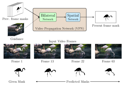
In this work, we focus on the problem of propagating structured information across video frames. This problem appears in many forms (e.g., semantic segmentation or depth estimation) and is a pre-requisite for many applications. An example instance is shown in Fig. 1. Given an object mask for the first frame, the problem is to propagate this mask forward through the entire video sequence. Propagation of semantic information through time and video color propagation are other problem instances.
Videos pose both technical and representational challenges. The presence of scene and camera motion lead to the difficult pixel association problem of optical flow. Video data is computationally more demanding than static images. A naive per-frame approach would scale at least linear with frames. These challenges complicate the use of standard convolutional neural networks (CNNs) for video processing. As a result, many previous works for video propagation use slow optimization based techniques.
We propose a generic neural network architecture that propagates information across video frames. The main innovation is the use of image adaptive convolutional operations that automatically adapts to the video stream content. This yields networks that can be applied to several types of information, e.g., labels, colors, etc. and runs online, that is, only requiring current and previous frames.
Our architecture is composed of two components (see Fig. 1). A temporal bilateral network that performs image-adaptive spatio-temporal dense filtering. The bilateral network allows to connect densely all pixels from current and previous frames and to propagate associated pixel information to the current frame. The bilateral network allows the specification of a metric between video pixels and allows a straight-forward integration of temporal information. This is followed by a standard spatial CNN on the bilateral network output to refine and predict for the present video frame. We call this combination a Video Propagation Network (VPN). In effect, we are combining video-adaptive filtering with rather small spatial CNNs which leads to a favorable runtime compared to many previous approaches.
VPNs have the following suitable properties for video processing:
General applicability:
VPNs can be used to propagate any type of information content i.e., both discrete (e.g., semantic labels) and continuous (e.g., color) information across video frames.
Online propagation:
The method needs no future frames and can be used for online video analysis.
Long-range and image adaptive:
VPNs can efficiently handle a large number of input frames and are adaptive to the video with long-range pixel connections.
End-to-end trainable:
VPNs can be trained end-to-end, so they can be used in other deep network architectures.
Favorable runtime:
VPNs have favorable runtime in comparison to many current best methods, what makes them amenable for learning with large datasets.
Empirically we show that VPNs, despite being generic, perform better than published approaches on video object segmentation and semantic label propagation while being faster. VPNs can easily be integrated into sequential per-frame approaches and require only a small fine-tuning step that can be performed separately.
2 Related Work
General propagation techniques
Techniques for propagating content across image/video pixels are predominantly optimization based or filtering techniques. Optimization based techniques typically formulate the propagation as an energy minimization problem on a graph constructed across video pixels or frames. A classic example is the color propagation technique from [46]. Although efficient closed-form solutions [47] exists for some scenarios, optimization tends to be slow due to either large graph structures for videos and/or the use of complex connectivity. Fully-connected conditional random fields (CRFs) [41] open a way for incorporating dense and long-range pixel connections while retaining fast inference.
Filtering techniques [40, 15, 30] aim to propagate information with the use of image/video filters resulting in fast runtimes compared to optimization techniques. Bilateral filtering [5, 73] is one of the popular filters for long-range information propagation. A popular application is joint bilateral upsampling [40] that upsamples a low-resolution signal with the use of a high-resolution guidance image. The works of [51, 22, 37, 34, 81, 66] showed that one can back-propagate through the bilateral filtering operation for learning filter parameters [37, 34] or doing optimization in the bilateral space [8, 7]. Recently, several works proposed to do upsampling in images by learning CNNs that mimic edge-aware filtering [78] or that directly learn to upsample [49, 32]. Most of these works are confined to images and are either not extendable or computationally too expensive for videos. We leverage some of these previous works and propose a scalable yet robust neural network approach for video propagation. We will discuss more about bilateral filtering, that forms the core of our approach, in Section 3.
Video object segmentation
Prior work on video object segmentation can be broadly categorized into two types: Semi-supervised methods that require manual annotation to define what is foreground object and unsupervised methods that does segmentation completely automatically. Unsupervised techniques such as [25, 48, 45, 55, 77, 80, 72, 23] use some prior information about the foreground objects such as distinctive motion, saliency etc.
In this work, we focus on the semi-supervised task of propagating the foreground mask from the first frame to the entire video. Existing works predominantly use graph-based optimization that perform graph-cuts [9, 10, 69] on video. Several of these works [64, 50, 61, 76, 39, 33] aim to reduce the complexity of graph structure with clustering techniques such as spatio-temporal superpixels and optical flow [75]. Another direction was to estimate correspondence between different frame pixels [4, 6, 44] by using nearest neighbor fields [26] or optical flow [18]. Closest to our technique are the works of [60] and [53]. [60] proposed to use fully-connected CRF over the object proposals across frames. [53] proposed a graph-cut in the bilateral space. Instead of graph-cuts, we learn propagation filters in the high-dimensional bilateral space. This results in a more generic architecture and allows integration into other deep networks. Two contemporary works [14, 36] proposed CNN based approaches for object segmentation and rely on fine-tuning a deep network using the first frame annotation of a given test sequence. This could result in overfitting to the test background. In contrast, the proposed approach relies only on offline training and thus can be easily adapted to different problem scenarios as demonstrated in this paper.
Semantic video segmentation
Earlier methods such as [12, 70] use structure from motion on video frames to compute geometrical and/or motion features. More recent works [24, 16, 19, 54, 74, 43] construct large graphical models on videos and enforce temporal consistency across frames. [16] used dynamic temporal links in their CRF energy formulation. [19] proposes to use Perturb-and-MAP random field model with spatial-temporal energy terms and [54] propagate predictions across time by learning a similarity function between pixels of consecutive frames.
In the recent years, there is a big leap in the performance of semantic segmentation [52, 17] with the use of CNNs but mostly applied to images. Recently, [67] proposed to retain the intermediate CNN representations while sliding a image CNN across the frames. Another approach is to take unary predictions from CNN and then propagate semantic information across the frames. A recent prominent approach in this direction is of [43] which proposes a technique for optimizing feature spaces for fully-connected CRF.
3 Bilateral Filtering
We briefly review the bilateral filtering and its extensions that we will need to build VPN. Bilateral filtering has its roots in image denoising [5, 73] and has been developed as an edge-preserving filter. It has found numerous applications [58] and recently found its way into neural network architectures [81, 27]. We will use this filtering at the core of VPN and make use of the image/video-adaptive connectivity as a way to cope with scenes in motion.
Let represent a scalar, vector and matrix respectively. Bilateral filtering a vectorized image having image pixels can be viewed as a matrix-vector multiplication with a filter matrix :
| (1) |
where the filter weights depend on features at input pixel indices and for -dimensional features. For example a Gaussian bilateral filter amounts to a particular choice of as , where is a normalization constant and is covariance matrix. The choice of features define the effect of the filter, the way it adapts to image content. To use only positional features, , the bilateral filter operation reduces to a spatial Gaussian filter, with width controlled by . A common choice for edge-preserving filtering is to choose color and position features . This results in image smoothing without blurring across the edges.
The filter values change for every pixel pairs and depend on the image/video content. And since the number of image/video pixels is usually large, a naive implementation of Eq. 1 is prohibitive. Due to the importance of this filtering operation, several fast algorithms [2, 3, 57, 28] have been proposed, that directly computes Eq. 1 without explicitly building matrix. One natural view that inspired several implementations was offered by [57], who viewed the bilateral filtering operation as a computation in a higher dimensional space. Their observation was that bilateral filtering can be implemented by 1. projecting into a high-dimensional grid (splatting) defined by features , 2. high-dimensional filtering (convolving) the projected signal and 3. projecting down the result at the points of interest (slicing). The high-dimensional grid is also called bilateral space/grid. All these operations are linear and written as:
| (2) |
where, and denotes the mapping to-from image pixels and bilateral grid, and denotes convolution (traditionally Gaussian) in the bilateral space. The bilateral space has same dimensionality as features . The problem with this approach is that a standard -dimensional convolution on a regular grid requires handling of an exponential number of grid points. This was circumvented by a special data structure, the permutohedral lattice as proposed in [2]. Effectively permutohedral filtering scales linearly with dimension, resulting in fast execution time.
The recent work of [37, 34] then generalized the bilateral filter in the permutohedral lattice and demonstrated how it can be learned via back-propagation. This allowed the construction of image-adaptive filtering operations into deep learning architectures, which we will build upon. See Fig. 2 for a illustration of 2D permutohedral lattices. Refer to [2] for more details on bilateral filtering using permutohedral lattice and refer to [34] for details on learning general permutohedral filters via back-propagation.

4 Video Propagation Networks
We aim to adapt the bilateral filtering operation to predict information forward in time, across video frames. Formally, we work on a sequence of (color or grayscale) images and denote with a sequence of outputs, one per frame. Consider as an example a sequence of foreground masks for a moving object in the scene. Our goal is to develop an online propagation method that can predict , having observed the video up to frame and possibly previous
| (3) |
If training examples with full or partial knowledge of are available, it is possible to learn and for a complex and unknown input-output relationship, a deep CNN is a natural design choice. However, any learning based method has to face the challenge: the scene/camera motion and its effect on . Since no motion in two different videos is the same, fixed-size static receptive fields of CNN are insufficient. We propose to resolve this with video-adaptive filtering component, an adaption of the bilateral filtering to videos. Our Bilateral Network (Section 4.1) has a connectivity that adapts to video sequences, its output is then fed into a spatial Network (Section 4.2) that further refines the desired output. The combined network layout of this VPN is depicted in Fig. 3. It is a sequence of learnable bilateral and spatial filters that is efficient, trainable end-to-end and adaptive to the video input.
4.1 Bilateral Network (BNN)
Several properties of bilateral filtering make it a perfect candidate for information propagation in videos. In particular, our method is inspired by two main ideas that we extend in this work: joint bilateral upsampling [40] and learnable bilateral filters [34]. Although, bilateral filtering has been used for filtering video data before [56], its use has been limited to fixed filter weights (say, Gaussian).
Fast Bilateral Upsampling across Frames The idea of joint bilateral upsampling [40] is to view upsampling as a filtering operation. A high resolution guidance image is used to upsample a low-resolution result. In short, a smaller number of input points are given , for example a segmentation result at a lower resolution with the corresponding guidance image features . This is then scaled to a larger number of output points with features using the bilateral filtering operation, that is to compute Eq. 1, where the sum runs over all points and the output is computed for all positions ().
We will use this idea to propagate content from previous frames () to the current frame (). The summation in Eq. 1 now runs over all previous frames and pixels. This is illustrated in Fig. 2. We take all previous frame results and splat them into a lattice using the features computed on video frames . A filtering (described below) is then applied to every lattice point and the result is then sliced back using the features of the current frame . This result need not be the final , in fact we compute a filter bank of responses and continue with further processing as will be discussed.
Standard bilateral features used for images need not be optimal for videos. A recent work of [43] propose to optimize bilateral feature spaces for videos. Instead, we choose to simply add frame index as an additional time feature yielding a 6 dimensional feature vector for every video pixel. Imagine a video where an object moves to reveal some background. Pixels of the object and background will be close spatially and temporally but likely be of different color . Therefore they will have no strong influence on each other (being splatted to distant positions in the six-dimensional bilateral space). One can understand the filter to be adaptive to color changes across frames, only pixels that are static and have similar color have a strong influence on each other (end up nearby in the bilateral space). In all our experiments, we used time as additional feature for information propagation across frames.
In addition to adding time as additional feature, we also experimented with using optical flow. We make use of optical flow estimates (of the previous frames with respect to the current frame) by warping pixel position features of previous frames by their optical flow displacement vectors to . If the perfect flow was available, the video frames could be warped into a common frame of reference. This would resolve the corresponding problem and make information propagation much easier. We refer to the VPN model that uses modified positional features as VPN-Flow.
Another property of permutohedral filtering that we exploit is that the input points need not lie on a regular grid since the filtering is done in the high-dimensional lattice. Instead of splatting millions of pixels on to the lattice, we randomly sample or use superpixels and perform filtering using these sampled points as input to the filter. In practice, we observe that this results in big computational gains with minor drop in performance (more in Section 5.1).

Learnable Bilateral Filters Bilateral filters help in video-adaptive information propagation across frames. But the standard Gaussian filter may be insufficient and further, we would like to increase the capacity by using a filter bank instead of a single fixed filter. We propose to use the technique of [34] to learn a filter bank in the permutohedral lattice using back-propagation.
The process works as follows. A input video is used to determine the positions in the bilateral space to splat the input points of the previous frames. In a general case, need not be a scalar and let us assume . The features (e.g. ) define the splatting matrix . This leads to a number of vectors , that lie on the permutohedral lattice, with dimensionality . In effect, the splatting operation groups points that are close together, that is, they have similar . All lattice points are now filtered using a filter bank which results in dimensional vectors on the lattice points. These are sliced back to the points of interest (present video frame). The values of are learned by back-propagation. General parametrization of from [34, 37] allows to have any neighborhood size for the filters. Since constructing the neighborhood structure in high-dimensions is time consuming, we choose to use filters for speed reasons. These three steps of splatting, convolving and slicing makes up one Bilateral Convolution Layer (BCL) which we will stack and concatenate to form a Bilateral Network. See Fig. 2 for a BCL illustration.
BNN Architecture The Bilateral Network (BNN) is illustrated in the green box of Fig. 3. The input is a video sequence and the corresponding predictions up to frame . Those are filtered using two BCLs (BCLa, BCLb) with filters each. For both BCLs, we use the same features but scale them with different diagonal matrices: . The feature scales () are found by validation. The two dimensional outputs are concatenated, passed through a ReLU non-linearity and passed to a second layer of two separate BCL filters that uses same feature spaces . The output of the second filter bank is then reduced using a spatial filter to map to the original dimension of . We investigated scaling frame inputs with an exponential time decay and found that, when processing frame , a re-weighting with with improved the performance a little bit.
In the experiments, we also included a simple BNN variant, where no filters are applied inside the permutohedral space, just splatting and slicing with the two layers BCLa and BCLb and adding the results. We will refer to this model as BNN-Identity as this is equivalent to using filter that is identity matrix. It corresponds to an image adaptive smoothing of the inputs . We found this filtering to already have a positive effect in our experiments.
4.2 Spatial Network
The BNN was designed to propagate information from the previous frames to the present one, respecting the scene and object motion. We then add a small spatial CNN with 3 layers, each with filters of size , interleaved with ReLU non-linearities. The final result is then mapped to the desired output of using a convolution. The main role of this spatial CNN is to refine the information in frame . Depending on the problem and the size of the available training data, other network designs are conceivable. We use the same network architecture shown in Fig. 3 for all the experiments to demonstrate the generality of VPNs.
5 Experiments
We evaluated VPN on three different propagation tasks: propagation of foreground masks, semantic labels and color in videos. Our implementation runs in Caffe [35] using standard settings. We used Adam [38] stochastic optimization for training VPNs, multinomial-logistic loss for label propagation networks and Euclidean loss for training color propagation networks. We use a fixed learning rate of 0.001 and choose the trained models with minimum validation loss. Runtime computations were performed using a Nvidia TitanX GPU and a 6 core Intel i7-5820K CPU clocked at 3.30GHz machine. The code is available online at http://varunjampani.github.io/vpn/.
5.1 Video Object Segmentation
We focus on the semi-supervised task of propagating a given first frame foreground mask to all the video frames. Object segmentation in videos is useful for several high level tasks such as video editing, rotoscoping etc.
Dataset
We use the recently published DAVIS dataset [59] for experiments on this task. It consists of 50 high-quality videos. All the frames come with high-quality per-pixel annotation of the foreground object. For robust evaluation and to get results on all the dataset videos, we evaluate our technique using 5-fold cross-validation. We randomly divided the data into 5 folds, where in each fold, we used 35 videos for training, 5 for validation and the remaining 10 for the testing. For the evaluation, we used the 3 metrics that are proposed in [59]: Intersection over Union (IoU) score, Contour accuracy () score and temporal instability () score. The widely used IoU score is defined as , where TP: True Positives; FN: False Negatives and FP: False Positives. Refer to [59] for the definition of the other two metrics.
| F-1 | F-2 | F-3 | F-4 | F-5 | All | |
|---|---|---|---|---|---|---|
| BNN-Identity | 56.4 | 74.0 | 66.1 | 72.2 | 66.5 | 67.0 |
| VPN-Stage1 | 58.2 | 77.7 | 70.4 | 76.0 | 68.1 | 70.1 |
| VPN-Stage2 | 60.9 | 78.7 | 71.4 | 76.8 | 69.0 | 71.3 |
| IoU | Runtime(s) | |||
| BNN-Identity | 67.0 | 67.1 | 36.3 | 0.21 |
| VPN-Stage1 | 70.1 | 68.4 | 30.1 | 0.48 |
| VPN-Stage2 | 71.3 | 68.9 | 30.2 | 0.75 |
| With pre-trained models | ||||
| DeepLab | 57.0 | 49.9 | 47.8 | 0.15 |
| VPN-DeepLab | 75.0 | 72.4 | 29.5 | 0.63 |
| OFL [75] | 71.1 | 67.9 | 22.1 | 60 |
| BVS [53] | 66.5 | 65.6 | 31.6 | 0.37 |
| NLC [25] | 64.1 | 59.3 | 35.6 | 20 |
| FCP [60] | 63.1 | 54.6 | 28.5 | 12 |
| JMP [26] | 60.7 | 58.6 | 13.2 | 12 |
| HVS [29] | 59.6 | 57.6 | 29.7 | 5 |
| SEA [62] | 55.6 | 53.3 | 13.7 | 6 |
VPN and Results
In this task, we only have access to foreground mask for the first frame . For the ease of training VPN, we obtain initial set of predictions with BNN-Identity. We sequentially apply BNN-Identity at each frame and obtain an initial set of foreground masks for the entire video. These BNN-Identity propagated masks are then used as inputs to train a VPN to predict the refined masks at each frame. We refer to this VPN model as VPN-Stage1. Once VPN-Stage1 is trained, its refined mask predictions are in-turn used as inputs to train another VPN model which we refer to as VPN-Stage2. This resulted in further refinement of foreground masks. Training further stages did not result in any improvements. Instead, one could consider VPN as a RNN unit processing one frame after another. But, due to GPU memory constraints, we opted for stage-wise training.
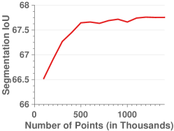
Following the recent work of [53] on video object segmentation, we used features with YCbCr color features for bilateral filtering. To be comparable with one of the fastest state-of-the-art technique [53], we do not use any optical flow information. First, we analyze the performance of BNN-Identity by changing the number of randomly sampled input points. Figure 4 shows how the segmentation IoU changes with the number of sampled points (out of 2 million points) from the previous frames. The IoU levels out after sampling 25% of the points. For further computational efficiency, we used superpixel sampling instead of random sampling. Compared to random sampling, usage of superpixels reduced the IoU slightly (0.5), while reducing the number of input points by a factor of 10. We used 12000 SLIC [1] superpixels from each frame computed using the fast GPU implementation from [63]. As an input to VPN, we use the mask probabilities of previous 9 frames as we observe no improvements with more frames. We set and the feature scales () are presented in Tab. A.1.
Table 1 shows the IoU scores for each of the 5 folds and Tab. 2 shows the overall scores and runtimes of different VPN models along with the best performing techniques. The performance improved consistently across all 5 folds with the addition of new VPN stages. BNN-Identity already performed reasonably well. VPN outperformed the present fastest BVS method [53] by a significant margin on all the performance measures while being comparable in runtime. VPN perform marginally better than OFL method [75] while being at least 80 faster and OFL relies on optical flow whereas we obtain similar performance without using any optical flow. Further, VPN has the advantage of doing online processing as it looks only at previous frames whereas BVS processes entire video at once.
Augmentation of Pre-trained Models
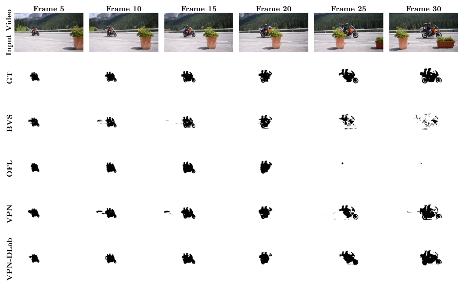
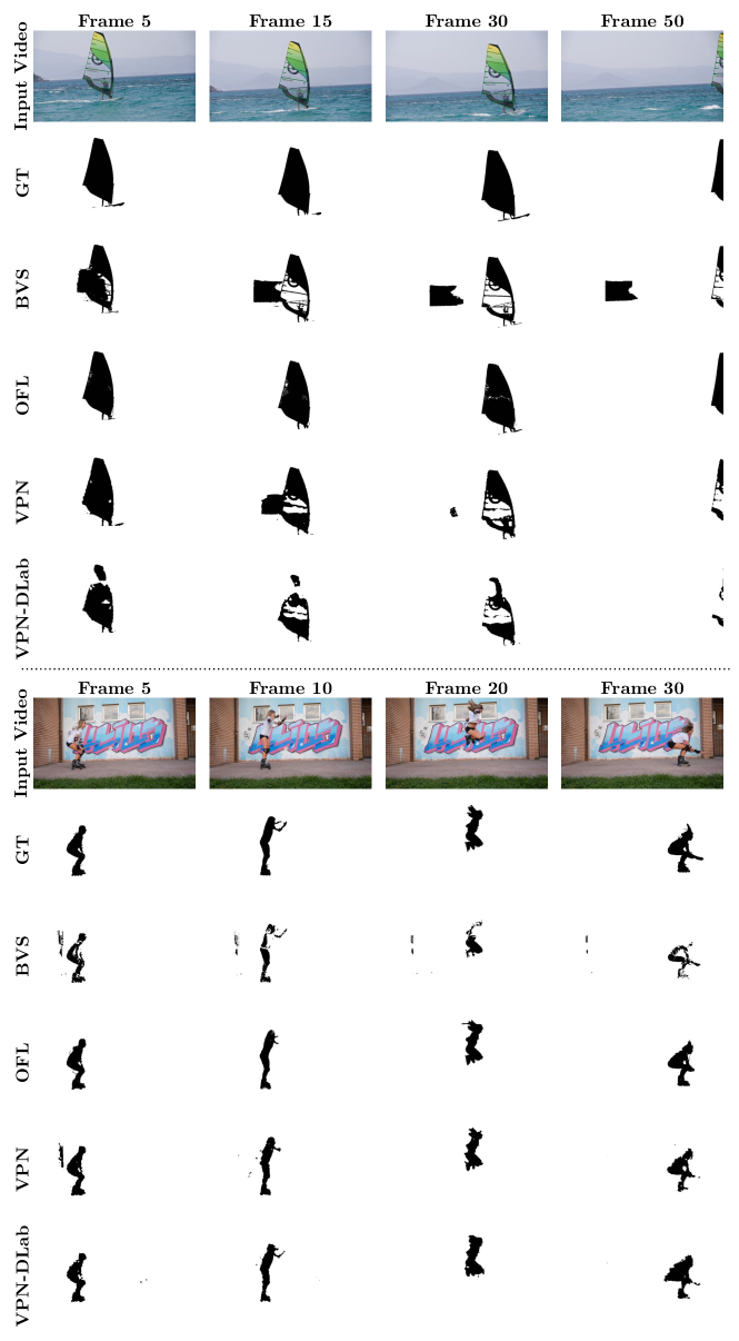
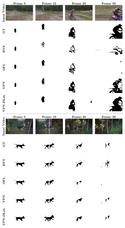
One of the main advantages of VPN is that it is end-to-end trainable and can be easily integrated into other deep networks. To demonstrate this, we augmented VPN architecture with standard DeepLab segmentation network [17]. We replaced the last classification layer of DeepLab-LargeFOV model to output 2 classes (foreground and background) in our case and bi-linearly upsampled the resulting low-resolution probability map to the original image dimension. 5-fold fine-tuning of the DeepLab model on DAVIS dataset resulted in the average IoU of 57.0 and other scores are shown in Tab. 2. To construct a joint model, the outputs from the DeepLab and the bilateral network (in VPN) are concatenated and then passed on to the spatial CNN. In other words, the bilateral network propagates label information from previous frames to the present frame, whereas the DeepLab network does the prediction for the present frame. The results of both are then combined and refined by the spatial network in the VPN. We call this ‘VPN-DeepLab’ model. We trained this model end-to-end and observed big improvements in performance. As shown in Tab. 2, the VPN-DeepLab model has the IoU score of 75.0 which is a significant improvement over the published results. The total runtime of VPN-DeepLab is only 0.63s which makes this also one of the fastest techniques. Figure 5 shows some qualitative results with more in Figs. A.1, A.2 and A.3. One can obtain better VPN performance with using better superpixels and also incorporating optical flow, but this increases runtime as well. Visual results indicate that learned VPN is able to retain foreground masks even with large variations in viewpoint and object size.
5.2 Semantic Video Segmentation
This is the task of assigning semantic label to every video pixel. Since the semantics between adjacent frames does not change radically, intuitively, propagating semantics across frames should improve the segmentation quality of each frame. Unlike video object segmentation, where the mask for the first frame is given, we approach semantic video segmentation in a fully automatic fashion. Specifically, we start with the unary predictions of standard CNNs and use VPN for propagating semantics across the frames.
Dataset
We use the CamVid dataset [11] that contains 4 high quality videos captured at 30Hz while the semantically labeled 11-class ground truth is provided at 1Hz. While the original dataset comes at a resolution of 960720, we operate on a resolution of 640480 as in [79, 43]. We use the same splits as in [70] resulting in 367, 100 and 233 frames with ground truth for training, validation and testing.
VPN and Results
Since we already have CNN predictions for every frame, we train a VPN that takes the CNN predictions of previous and present frames as input and predicts the refined semantics for the present frame. We compare with a state-of-the-art CRF approach [43] which we refer to as FSO-CRF. We also experimented with optical flow in VPN and refer that model as VPN-Flow. We used the fast DIS optical flow [42] and modify the positional features of previous frames. We used superpixels computed with Dollar et al. [20] as gSLICr [63] has introduced artifacts.
| IoU | Runtime(s) | |
| CNN-1 from [79] | 65.3 | 0.38 |
| + FSO-CRF [43] | 66.1 | 10 |
| + BNN-Identity | 65.3 | 0.31 |
| + BNN-Identity-Flow | 65.5 | 0.33 |
| + VPN (Ours) | 66.5 | 0.35 |
| + VPN-Flow (Ours) | 66.7 | 0.37 |
| CNN-2 from [65] | 68.9 | 0.30 |
| + VPN-Flow (Ours) | 69.5 | 0.38 |
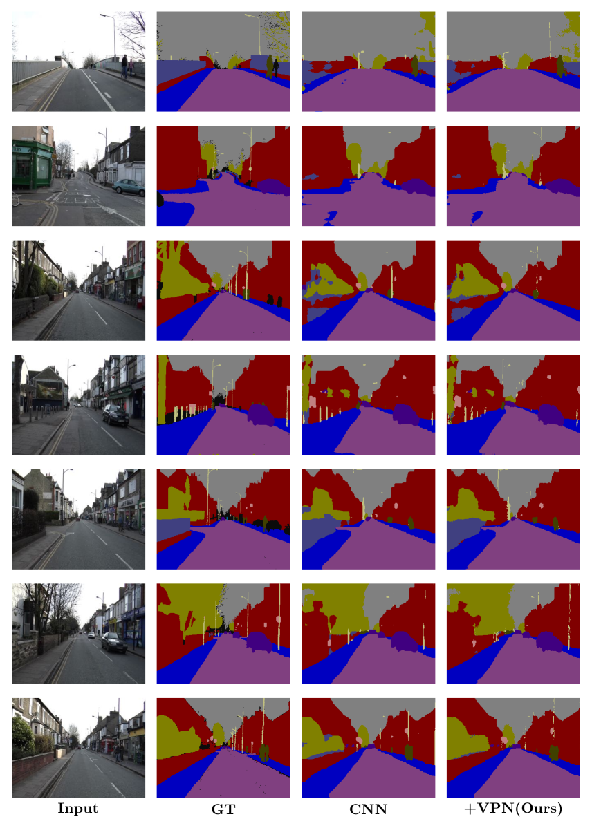
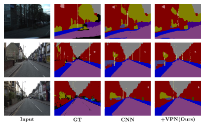
We experimented with predictions from two different CNNs: One is with dilated convolutions [79] (CNN-1) and another one [65] (CNN-2) is trained with the additional video game data, which is the present state-of-the-art on this dataset. For CNN-1 and CNN-2, using 2 and 3 previous frames respectively as input to VPN is found to be optimal. Other parameters of VPN are presented in Tab. A.1. Table 3 shows quantitative results. Using BNN-Identity only slightly improved the performance whereas training the entire VPN significantly improved the CNN-1 performance by over 1.2 IoU, with both VPN and VPN-Flow. Moreover, VPN is at least 25 faster, and simpler to use compared to the optimization based FSO-CRF which relies on LDOF optical flow [13], long-term tacks [71] and edges [21]. Replacing bilateral filters with spatial filters in VPN improved the CNN-1 performance by only 0.3 IoU showing the importance of video-adaptive filtering. We further improved the performance of the state-of-the-art CNN-2 [65] with VPN-Flow model. Using better optical flow estimation might give even better results. Figure 6 shows some qualitative results with more in Fig. A.4.
5.3 Video Color Propagation
We also evaluate VPNs on a regression task of propagating color information in a grayscale video. Given the color image for the first video frame, the task is to propagate the color to the entire video. For experiments on this task, we again used the DAVIS segmentation dataset [59] with the first 25 frames from each video. We randomly divided the dataset into 30 train, 5 validation and 15 test videos.
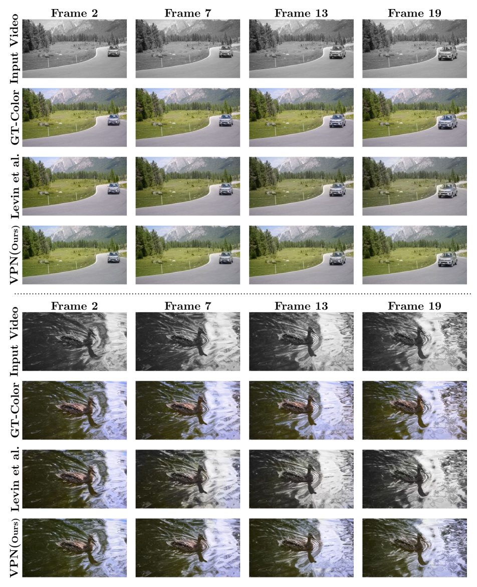
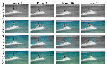
We work with YCbCr representation of images and propagate CbCr values from previous frames with pixel intensity, position and time features as guidance for VPN. The same strategy as in object segmentation is used, where an initial set of color propagated results is obtained with BNN-Identity and then used to trained a VPN-Stage1 model. Training further VPN stages did not improve the performance. We use 300K randomly sampled points from previous 3 frames as input to the VPN network. Table 4 shows the PSNR results. We also show a baseline result of [46] that does graph based optimization using optical flow. We used fast DIS optical flow [42] in the baseline method [46] and we did not observe significant differences with using LDOF optical flow [13]. Figure 7 shows a visual result with more in Fig. A.5. VPN works reliably better than [46] while being 20 faster. The method of [46] relies heavily on optical flow and so the color drifts away with incorrect flow. We observe that our method also bleeds color in some regions especially when there are large viewpoint changes. We could not compare against recent color propagation techniques [31, 68] as their codes are not available online. This application shows general applicability of VPNs in propagating different kinds of information.
| PSNR | Runtime(s) | |
|---|---|---|
| BNN-Identity | 27.89 | 0.29 |
| VPN-Stage1 | 28.15 | 0.90 |
| Levin et al. [46] | 27.11 | 19 |
6 Conclusion
We proposed a fast, scalable and generic neural network approach for propagating information across video frames. The VPN uses bilateral network for long-range video-adaptive propagation of information from previous frames to the present frame which is then refined by a spatial network. Experiments on diverse tasks show that VPNs, despite being generic, outperformed the current state-of-the-art task-specific methods. At the core of our technique is the exploitation and modification of learnable bilateral filtering for the use in video processing. We used a simple VPN architecture to showcase the generality. Depending on the problem and the availability of data, using more filters or deeper layers would result in better performance. In this work, we manually tuned the feature scales which could be amendable to learning. Finding optimal yet fast-to-compute bilateral features for videos together with the learning of their scales is an important future research direction.
Acknowledgments
We thank Vibhav Vineet for providing the trained image segmentation CNN models for CamVid dataset.
References
- [1] R. Achanta, A. Shaji, K. Smith, A. Lucchi, P. Fua, and S. Susstrunk. SLIC superpixels compared to state-of-the-art superpixel methods. Pattern Analysis and Machine Intelligence, IEEE Transactions on, 34(11):2274–2282, 2012.
- [2] A. Adams, J. Baek, and M. A. Davis. Fast high-dimensional filtering using the permutohedral lattice. In Computer Graphics Forum, volume 29, pages 753–762. Wiley Online Library, 2010.
- [3] A. Adams, N. Gelfand, J. Dolson, and M. Levoy. Gaussian kd-trees for fast high-dimensional filtering. ACM Transactions on Graphics (ToG), 28(3):21, 2009.
- [4] A. Agarwala, A. Hertzmann, D. H. Salesin, and S. M. Seitz. Keyframe-based tracking for rotoscoping and animation. ACM Transactions on Graphics (ToG), 23(3):584–591, 2004.
- [5] V. Aurich and J. Weule. Non-linear Gaussian filters performing edge preserving diffusion. In DAGM, pages 538–545. Springer, 1995.
- [6] X. Bai, J. Wang, D. Simons, and G. Sapiro. Video snapcut: robust video object cutout using localized classifiers. ACM Transactions on Graphics (TOG), 28(3):70, 2009.
- [7] J. T. Barron, A. Adams, Y. Shih, and C. Hernández. Fast bilateral-space stereo for synthetic defocus. In Computer Vision and Pattern Recognition, IEEE Conference on, pages 4466–4474, 2015.
- [8] J. T. Barron and B. Poole. The fast bilateral solver. In European Conference on Computer Vision. Springer, 2016.
- [9] Y. Boykov, O. Veksler, and R. Zabih. Fast approximate energy minimization via graph cuts. Pattern Analysis and Machine Intelligence, IEEE Transactions on, 23(11):1222–1239, 2001.
- [10] Y. Y. Boykov and M.-P. Jolly. Interactive graph cuts for optimal boundary & region segmentation of objects in nd images. In Proceedings of the IEEE International Conference on Computer Vision, volume 1, pages 105–112. IEEE, 2001.
- [11] G. J. Brostow, J. Fauqueur, and R. Cipolla. Semantic object classes in video: A high-definition ground truth database. Pattern Recognition Letters, 30(2):88–97, 2009.
- [12] G. J. Brostow, J. Shotton, J. Fauqueur, and R. Cipolla. Segmentation and recognition using structure from motion point clouds. In European Conference on Computer Vision, pages 44–57. Springer, 2008.
- [13] T. Brox, C. Bregler, and J. Malik. Large displacement optical flow. In Computer Vision and Pattern Recognition, IEEE Conference on, pages 41–48. IEEE, 2009.
- [14] S. Caelles, K.-K. Maninis, J. Pont-Tuset, L. Leal-Taixé, D. Cremers, and L. Van Gool. One-shot video object segmentation. arXiv preprint arXiv:1611.05198, 2016.
- [15] J.-H. R. Chang and Y.-C. F. Wang. Propagated image filtering. In Computer Vision and Pattern Recognition (CVPR), IEEE Conference on, pages 10–18. IEEE, 2015.
- [16] A. Y. Chen and J. J. Corso. Temporally consistent multi-class video-object segmentation with the video graph-shifts algorithm. In IEEE Winter Conference on Applications of Computer Vision, pages 614–621. IEEE, 2011.
- [17] L.-C. Chen, G. Papandreou, I. Kokkinos, K. Murphy, and A. L. Yuille. Semantic image segmentation with deep convolutional nets and fully connected crfs. arXiv preprint arXiv:1412.7062, 2014.
- [18] Y.-Y. Chuang, A. Agarwala, B. Curless, D. H. Salesin, and R. Szeliski. Video matting of complex scenes. ACM Transactions on Graphics (ToG), 21(3):243–248, 2002.
- [19] R. de Nijs, S. Ramos, G. Roig, X. Boix, L. Van Gool, and K. Kühnlenz. On-line semantic perception using uncertainty. In 2012 IEEE/RSJ International Conference on Intelligent Robots and Systems, pages 4185–4191. IEEE, 2012.
- [20] P. Dollár and C. L. Zitnick. Structured forests for fast edge detection. In Proceedings of the IEEE International Conference on Computer Vision, 2013.
- [21] P. Dollár and C. L. Zitnick. Fast edge detection using structured forests. Pattern Analysis and Machine Intelligence, IEEE Transactions on, 37(8):1558–1570, 2015.
- [22] J. Domke. Learning graphical model parameters with approximate marginal inference. Pattern Analysis and Machine Intelligence, IEEE Transactions on, 35(10):2454–2467, 2013.
- [23] R. Dondera, V. Morariu, Y. Wang, and L. Davis. Interactive video segmentation using occlusion boundaries and temporally coherent superpixels. In IEEE Winter Conference on Applications of Computer Vision, pages 784–791. IEEE, 2014.
- [24] A. Ess, T. Mueller, H. Grabner, and L. J. Van Gool. Segmentation-based urban traffic scene understanding. In British Machine Vision Conference, 2009.
- [25] A. Faktor and M. Irani. Video segmentation by non-local consensus voting. In BMVC, volume 2, page 6, 2014.
- [26] Q. Fan, F. Zhong, D. Lischinski, D. Cohen-Or, and B. Chen. Jumpcut: non-successive mask transfer and interpolation for video cutout. ACM Transactions on Graphics (ToG), 34(6):195, 2015.
- [27] R. Gadde, V. Jampani, M. Kiefel, D. Kappler, and P. Gehler. Superpixel convolutional networks using bilateral inceptions. In European Conference on Computer Vision. Springer, 2016.
- [28] E. S. Gastal and M. M. Oliveira. Domain transform for edge-aware image and video processing. ACM Transactions on Graphics (ToG), 30(4):69, 2011.
- [29] M. Grundmann, V. Kwatra, M. Han, and I. Essa. Efficient hierarchical graph-based video segmentation. In Computer Vision and Pattern Recognition, IEEE Conference on, pages 2141–2148. IEEE, 2010.
- [30] K. He, J. Sun, and X. Tang. Guided image filtering. In European Conference on Computer Vision, pages 1–14. Springer, 2010.
- [31] J.-H. Heu, D.-Y. Hyun, C.-S. Kim, and S.-U. Lee. Image and video colorization based on prioritized source propagation. In 2009 16th IEEE International Conference on Image Processing (ICIP), pages 465–468. IEEE, 2009.
- [32] T.-W. Hui, C. C. Loy, and X. Tang. Depth map super-resolution by deep multi-scale guidance. In European Conference on Computer Vision, pages 353–369. Springer, 2016.
- [33] S. D. Jain and K. Grauman. Supervoxel-consistent foreground propagation in video. In European Conference on Computer Vision, pages 656–671. Springer, 2014.
- [34] V. Jampani, M. Kiefel, and P. V. Gehler. Learning sparse high dimensional filters: Image filtering, dense CRFs and bilateral neural networks. In Computer Vision and Pattern Recognition, IEEE Conference on, June 2016.
- [35] Y. Jia, E. Shelhamer, J. Donahue, S. Karayev, J. Long, R. Girshick, S. Guadarrama, and T. Darrell. Caffe: Convolutional architecture for fast feature embedding. In Proceedings of the ACM International Conference on Multimedia, pages 675–678. ACM, 2014.
- [36] A. Khoreva, F. Perazzi, R. Benenson, B. Schiele, and A. Sorkine-Hornung. Learning video object segmentation from static images. arXiv preprint arXiv:1612.02646, 2016.
- [37] M. Kiefel, V. Jampani, and P. V. Gehler. Permutohedral lattice CNNs. International Conference on Learning Representations Workshop, 2015.
- [38] D. Kingma and J. Ba. Adam: A method for stochastic optimization. International Conference on Learning Representations, 2015.
- [39] P. Kohli and P. H. Torr. Dynamic graph cuts for efficient inference in markov random fields. Pattern Analysis and Machine Intelligence, IEEE Transactions on, 29(12):2079–2088, 2007.
- [40] J. Kopf, M. F. Cohen, D. Lischinski, and M. Uyttendaele. Joint bilateral upsampling. ACM Transactions on Graphics (ToG), 26(3):96, 2007.
- [41] P. Krähenbühl and V. Koltun. Efficient inference in fully connected CRFs with Gaussian edge potentials. In Advances in neural information processing systems, 2011.
- [42] T. Kroeger, R. Timofte, D. Dai, and L. Van Gool. Fast optical flow using dense inverse search. In European Conference on Computer Vision. Springer, 2016.
- [43] A. Kundu, V. Vineet, and V. Koltun. Feature space optimization for semantic video segmentation. In Computer Vision and Pattern Recognition, IEEE Conference on, 2016.
- [44] M. Lang, O. Wang, T. O. Aydin, A. Smolic, and M. H. Gross. Practical temporal consistency for image-based graphics applications. ACM Transactions on Graphics (ToG), 31(4):34–1, 2012.
- [45] Y. J. Lee, J. Kim, and K. Grauman. Key-segments for video object segmentation. In Proceedings of the IEEE International Conference on Computer Vision, pages 1995–2002. IEEE, 2011.
- [46] A. Levin, D. Lischinski, and Y. Weiss. Colorization using optimization. ACM Transactions on Graphics (ToG), 23(3):689–694, 2004.
- [47] A. Levin, D. Lischinski, and Y. Weiss. A closed-form solution to natural image matting. Pattern Analysis and Machine Intelligence, IEEE Transactions on, 30(2):228–242, 2008.
- [48] F. Li, T. Kim, A. Humayun, D. Tsai, and J. M. Rehg. Video segmentation by tracking many figure-ground segments. In Proceedings of the IEEE International Conference on Computer Vision, pages 2192–2199, 2013.
- [49] Y. Li, J.-B. Huang, N. Ahuja, and M.-H. Yang. Deep joint image filtering. In European Conference on Computer Vision, pages 154–169. Springer, 2016.
- [50] Y. Li, J. Sun, and H.-Y. Shum. Video object cut and paste. ACM Transactions on Graphics (ToG), 24(3):595–600, 2005.
- [51] Y. Li and R. Zemel. Mean-field networks. arXiv preprint arXiv:1410.5884, 2014.
- [52] J. Long, E. Shelhamer, and T. Darrell. Fully convolutional networks for semantic segmentation. In Computer Vision and Pattern Recognition, IEEE Conference on, pages 3431–3440, 2015.
- [53] N. Märki, F. Perazzi, O. Wang, and A. Sorkine-Hornung. Bilateral space video segmentation. In Computer Vision and Pattern Recognition, IEEE Conference on, pages 743–751, 2016.
- [54] O. Miksik, D. Munoz, J. A. Bagnell, and M. Hebert. Efficient temporal consistency for streaming video scene analysis. In Robotics and Automation (ICRA), 2013 IEEE International Conference on, pages 133–139. IEEE, 2013.
- [55] A. Papazoglou and V. Ferrari. Fast object segmentation in unconstrained video. In Proceedings of the IEEE International Conference on Computer Vision, pages 1777–1784, 2013.
- [56] S. Paris. Edge-preserving smoothing and mean-shift segmentation of video streams. In European Conference on Computer Vision, pages 460–473. Springer, 2008.
- [57] S. Paris and F. Durand. A fast approximation of the bilateral filter using a signal processing approach. In European Conference on Computer Vision, pages 568–580. Springer, 2006.
- [58] S. Paris, P. Kornprobst, J. Tumblin, and F. Durand. Bilateral filtering: Theory and applications. Now Publishers Inc, 2009.
- [59] F. Perazzi, J. Pont-Tuset, B. McWilliams, L. V. Gool, M. Gross, and A. Sorkine-Hornung. A benchmark dataset and evaluation methodology for video object segmentation. In Computer Vision and Pattern Recognition, IEEE Conference on, 2016.
- [60] F. Perazzi, O. Wang, M. Gross, and A. Sorkine-Hornung. Fully connected object proposals for video segmentation. In Proceedings of the IEEE International Conference on Computer Vision, pages 3227–3234, 2015.
- [61] B. L. Price, B. S. Morse, and S. Cohen. Livecut: Learning-based interactive video segmentation by evaluation of multiple propagated cues. In Proceedings of the IEEE International Conference on Computer Vision, pages 779–786. IEEE, 2009.
- [62] S. A. Ramakanth and R. V. Babu. Seamseg: Video object segmentation using patch seams. In Computer Vision and Pattern Recognition, IEEE Conference on, pages 376–383. IEEE, 2014.
- [63] C. Y. Ren, V. A. Prisacariu, and I. D. Reid. gslicr: Slic superpixels at over 250hz. ArXiv e-prints, (1509.04232), 2015.
- [64] M. Reso, B. Scheuermann, J. Jachalsky, B. Rosenhahn, and J. Ostermann. Interactive segmentation of high-resolution video content using temporally coherent superpixels and graph cut. In International Symposium on Visual Computing, pages 281–292. Springer, 2014.
- [65] S. R. Richter, V. Vineet, S. Roth, and V. Koltun. Playing for data: Ground truth from computer games. In European Conference on Computer Vision, pages 102–118. Springer, 2016.
- [66] A. G. Schwing and R. Urtasun. Fully connected deep structured networks. arXiv preprint arXiv:1503.02351, 2015.
- [67] E. Shelhamer, K. Rakelly, J. Hoffman, and T. Darrell. Clockwork convnets for video semantic segmentation. arXiv preprint arXiv:1608.03609, 2016.
- [68] B. Sheng, H. Sun, M. Magnor, and P. Li. Video colorization using parallel optimization in feature space. IEEE Transactions on Circuits and Systems for Video Technology, 24(3):407–417, 2014.
- [69] J. Shi and J. Malik. Normalized cuts and image segmentation. Pattern Analysis and Machine Intelligence, IEEE Transactions on, 22(8):888–905, 2000.
- [70] P. Sturgess, K. Alahari, L. Ladicky, and P. H. Torr. Combining appearance and structure from motion features for road scene understanding. In British Machine Vision Conference. BMVA, 2009.
- [71] N. Sundaram, T. Brox, and K. Keutzer. Dense point trajectories by gpu-accelerated large displacement optical flow. In European Conference on Computer Vision, pages 438–451. Springer, 2010.
- [72] B. Taylor, V. Karasev, and S. Soattoc. Causal video object segmentation from persistence of occlusions. In Computer Vision and Pattern Recognition, IEEE Conference on, pages 4268–4276. IEEE, 2015.
- [73] C. Tomasi and R. Manduchi. Bilateral filtering for gray and color images. In Proceedings of the IEEE International Conference on Computer Vision, pages 839–846. IEEE, 1998.
- [74] S. Tripathi, S. Belongie, Y. Hwang, and T. Nguyen. Semantic video segmentation: Exploring inference efficiency. In 2015 International SoC Design Conference (ISOCC), pages 157–158. IEEE, 2015.
- [75] Y.-H. Tsai, M.-H. Yang, and M. J. Black. Video segmentation via object flow. In Computer Vision and Pattern Recognition, IEEE Conference on, 2016.
- [76] J. Wang, P. Bhat, R. A. Colburn, M. Agrawala, and M. F. Cohen. Interactive video cutout. ACM Transactions on Graphics (ToG), 24(3):585–594, 2005.
- [77] W. Wang, J. Shen, and F. Porikli. Saliency-aware geodesic video object segmentation. In Computer Vision and Pattern Recognition, IEEE Conference on, pages 3395–3402, 2015.
- [78] L. Xu, J. S. Ren, Q. Yan, R. Liao, and J. Jia. Deep edge-aware filters. In Proceedings of the 32nd International Conference on Machine Learning, pages 1669–1678, 2015.
- [79] F. Yu and V. Koltun. Multi-scale context aggregation by dilated convolutions. International Conference on Learning Representations, 2016.
- [80] D. Zhang, O. Javed, and M. Shah. Video object segmentation through spatially accurate and temporally dense extraction of primary object regions. In Computer Vision and Pattern Recognition, IEEE Conference on, pages 628–635, 2013.
- [81] S. Zheng, S. Jayasumana, B. Romera-Paredes, V. Vineet, Z. Su, D. Du, C. Huang, and P. H. Torr. Conditional random fields as recurrent neural networks. In Proceedings of the IEEE International Conference on Computer Vision, 2015.
Appendix A Parameters and Additional Results
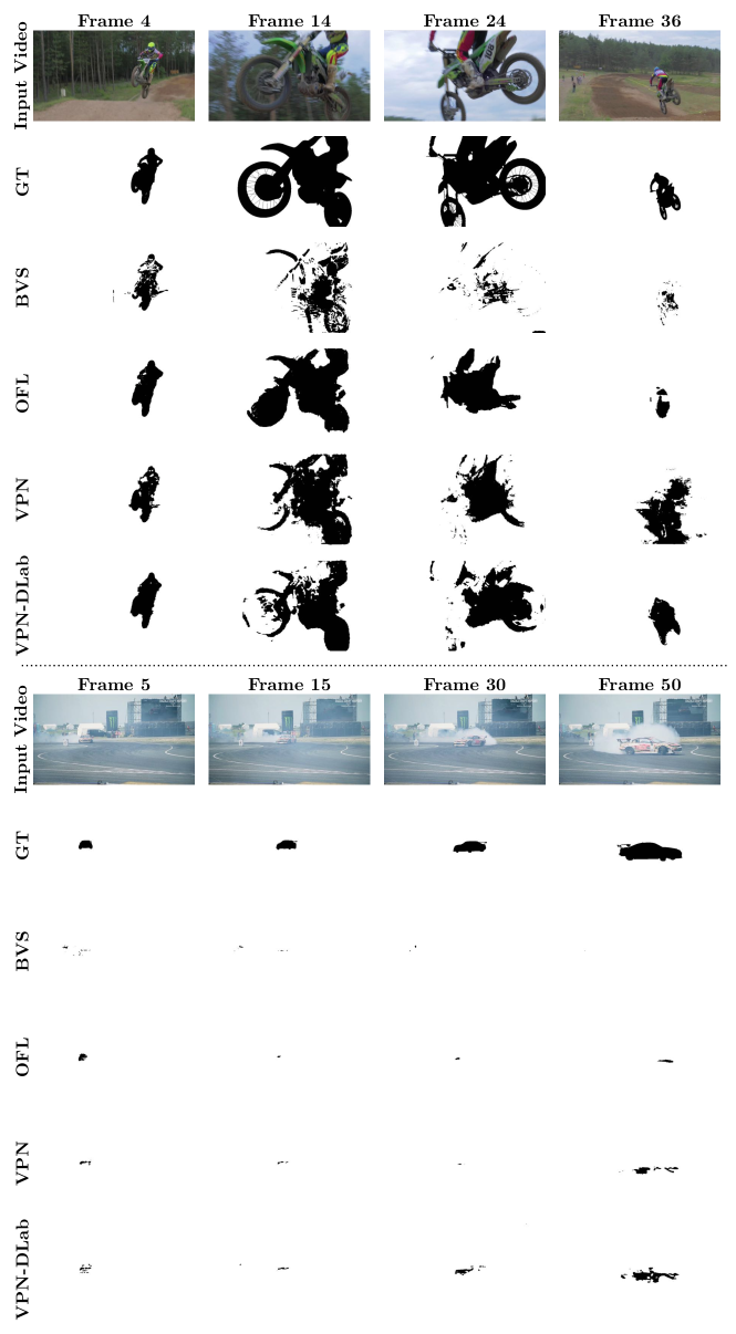
In this appendix, we present experiment protocols and additional qualitative results for experiments on video object segmentation, semantic video segmentation and video color propagation. Table A.1 shows the feature scales and other parameters used in different experiments. Figures A.1, A.2 show some qualitative results on video object segmentation with some failure cases in Fig. A.3. Figure A.4 shows some qualitative results on semantic video segmentation and Fig. A.5 shows results on video color propagation.
| Experiment | Feature Type | Feature Scale-1, | Feature Scale-2, | Input Frames | Loss Type | |
| Video Object Segmentation | () | (0.02,0.02,0.07,0.4,0.4,0.01) | (0.03,0.03,0.09,0.5,0.5,0.2) | 0.5 | 9 | Logistic |
| Semantic Video Segmentation | ||||||
| with CNN1 [79]-NoFlow | () | (0.08,0.08,0.2,0.2,0.2,0.04) | (0.11,0.11,0.2,0.2,0.2,0.04) | 0.5 | 3 | Logistic |
| with CNN1 [79]-Flow | () | (0.11,0.11,0.14,0.14,0.14,0.03) | (0.08,0.08,0.12,0.12,0.12,0.01) | 0.65 | 3 | Logistic |
| with CNN2 [65]-Flow | () | (0.08,0.08,0.2,0.2,0.2,0.04) | (0.09,0.09,0.25,0.25,0.25,0.03) | 0.5 | 4 | Logistic |
| Video Color Propagation | () | (0.04,0.04,0.2,0.04) | No second kernel | 1 | 4 | MSE |
