Evidence of reverse and intermediate size segregation in dry granular flows down a rough incline

Abstract

In a dry granular flow, size segregation had been shown to behave differently for a mixture containing a few large particles with a size ratio above 5 (N. Thomas, Phys. Rev. E 62, 961 (2000)). For moderately large size ratios, large particles migrate to an intermediate depth in the bed: this is called “intermediate segregation”. For the largest size ratios, large particles migrate down to the bottom of the flow: this is called “reverse segregation” - in contrast with surface segregation. As the reversal and intermediate depth values depend on the fraction of particles, this numerical study mainly uses one single large tracer. Small fractions of large beads are also computed showing the link between single tracer behavior and collective segregation process. For each device (half-filled rotating tumbler and rough plane), two (2D) and three (3D) dimensional cases are distinguished.

In the tumbler, the trajectories of a large tracer show that it reaches a constant depth during the flowing phase. For large size ratios, this depth is intermediate. A progressive sinking of the depth is obtained when the size ratio is increased. The largest size ratios correspond to tracers being at the bottom of the flowing layer. All 3D simulation results are in quantitative agreement with the experimental surface, intermediate, and reverse segregation results.

In the flow down a rough incline, a large tracer reaches an equilibrium depth during flow. For large size ratios, the depth is inside the bed, at an intermediate position, and for the largest size ratios, this depth is reverse, located near the bottom. Results are slightly different for a thin or a thick flow. For 3D thick flows, the reversal between surface and bottom positions occurs within a short range of size ratios: no tracer stabilizes near half-height and two reachable intermediate depth layers exist, below the surface and above the bottom reverse layer. For 3D thin flows, all intermediate depths are reachable by a tracer, depending on the size ratio. The numerical study of larger fractions of tracers (5 or 10%) shows the three segregation patterns (surface, intermediate, reverse) corresponding to the three types of equilibrium depth. The reversal is smoother than for a single tracer, and happens around the size ratio 4.5, in good agreement with experiments.

I Introduction

Size segregation in dry granular flow has been extensively studied as it is an important phenomenon occurring in natural flows or in industrial applications Williams76 ; DuranRajchenbach93 ; KnightJaeger93 ; CantelaubeBideau95 ; HutterVendsen96 ; OttinoKhaKhar00 ; GrayThornton06 ; SchlickFan15 . Recently, there have been significant advances in the modeling of segregation in dense granular flows. Models based on kinetic theory have been established for segregation in rapid flows, in the case of particles of different sizes and/or densities LarcherJenkins13 ; LarcherJenkins15 ; KhakharMcCarthy99 . These models, based on particle properties and with no adjustable parameter, are able to predict the evolution of the volume fraction of two types of particles that do not differ much in size or mass LarcherJenkins13 . Alternative models based on mixture theory have been proposed in which unequal stress partitioning reflects the mechanisms that are responsible for the segregation: kinetic sieving and squeeze expulsion SavageLun88 . In this continuum framework, particle segregation results from the lithostatic pressure gradient induced by gravity GrayThornton05 ; GrayThornton06 . Several groups have proposed improvements to take into account the effects of shear rate MayGolick10 ; TunuguntlaBokhove14 ; FanSchlick14 ; SchlickIsner16 , kinetic stress gradients (derived from vertical chutes) FanHill11 ; FanHill15 , or the polydispersity of flows with particles of different sizes and densities MarksRognon12 , leading to further developments for flows on inclines StaronPhillips16 . Quantitative agreement with experiments has been obtained for the stationary concentration profile of a mixture with a size ratio of 2 WiederseinerAncey11 . A comparative review can be found in TunuguntlaReview16 .

Most of these studies are concerned with small size ratios, the large particles being generally 1.5 to 2 times the size of the small ones. In some studies, size ratio is varied up to 3 FanSchlick14 , 3.5 Tunuguntla16 , or 4 GolickDaniels14 . This variation remains small compared with the size ratio range in our present study. Even so, it already induces a non-monotonic variation of some parameters, e.g. the segregation rate GolickDaniels14 . One of the studies concerning the measurement of the force acting on an object plunged into a granular flow Ding11 ; Ding13 ; Guillard14 provides interesting information on the segregation phenomenon because the intruder is free to move with the flow Guillard16 , instead of being an obstacle exerting drag. In these 2D simulations, the authors also noticed an extremum for the normalized segregation force obtained at the size ratio 2. Some segregation theory has been extended to large size ratios (up to 10) MarksRognon12 and predicts a monotonic decrease in the segregation time with the size ratio and without any change in the segregation pattern. Most of the models do not explicitly depend on the size ratio, but rather on a segregating velocity determined for each species TunuguntlaReview16 . In the few models where the size ratio is explicitly mentioned MarksRognon12 ; TunuguntlaBokhove14 , the segregating velocity cannot change sign when the size ratio is increased, for any particle fraction. In these models, only a difference in density between particles could induce a reversal of the segregating velocity direction TunuguntlaBokhove14 .

Nevertheless, the segregation phenomenon is observed to be different when increasing the size ratio above 4 or 5. It has been shown experimentally that large particles do not reach the surface, as they usually do in surface segregation, but move downwards and stabilize either at an intermediate depth or at the bottom of the flow for the largest size ratios Thomas00 . Particle stabilization at an intermediate depth has been named “intermediate segregation”. Large particle segregation at the bottom of the flow has been named “reverse segregation” by analogy with the “reverse Brazil-nut effect” ShinbrotMuzzio98 ; BreuEnsner03 ; EllenbergerVandu06 observed in vibrated granular systems. The origin of this vibrating effect HongQuinn01 is due to an inertia driven segregation process induced by high amplitude vibrations ShinbrotMuzzio98 ; HongQuinn01 as well as to the absence of convective motion knight93 . The reverse and intermediate segregations of particles of different sizes (and having the same density) have been observed experimentally in various sheared flows: channel flow, half-filled cylindrical rotating tumbler and 3D heap flow Thomas00 ; FelixThomas04 . The corresponding segregation patterns take different forms. In a rotating tumbler, if large particles are close to the tumbler center in the static part, reverse segregation occurs because particles move to the bottom of the flowing layer during flow. By contrast, tracers having a small size ratio (from 1.5 to 3) end up at the periphery on the solid part, undergoing surface segregation during flow. For a flow down an incline, the reverse-segregating large particles disappear from the surface during flow, and are present near the bottom of the deposit, while the surface-segregating large particles cover the flow and deposit surface. For a flow feeding a heap, very large beads form a vertical core (reverse segregation). For a small size ratio, a ring of large beads forms at the bottom periphery of the heap (surface segregation).

Intermediate segregation has been precisely observed in the tumbler: all large particles are found at the same intermediate radial position in the static part (Fig. 1) Thomas00 ; FelixThomas04 , forming a segregation half-ring pattern. An intermediate ring corresponds to an intermediate depth in the flowing layer (Fig. 2(a)). This was measured for size ratios ranging from 4 to approximately 15, for small fractions of large particles (3%) Thomas00 . In the experiments, the ring mean radius decreased continuously with increasing size ratios, corresponding in the flowing layer to a mean depth passing continuously from surface to bottom.

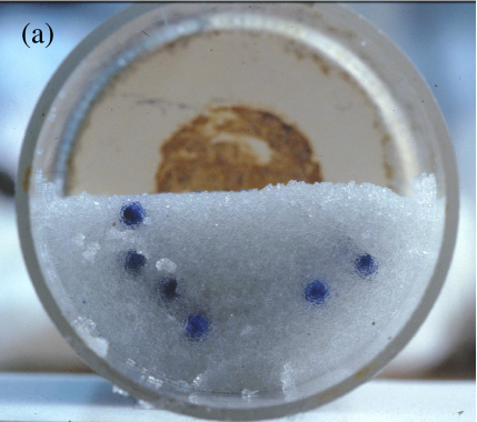
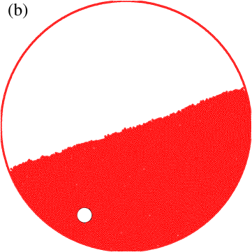
Figure 1: A $D=4.85$ cm rotating cylindrical tumbler with $d=0.3$ mm small particles and $d_{t}=$ 3 mm large particles (tracers): (a) cross-section of an experiment with 3% blue tracers, slowly impregnated with water after the flow has stopped, then sliced Thomas00 , (b) 2D simulation with one tracer.

The reversal of the segregation from the surface toward the bottom depends both on the size ratio and on the relative fraction of particles Thomas00 : a limit between surface and reverse segregations can be defined and it corresponds to a size ratio between 4 and 5 for small fractions (1 to 10%) of large particles; around 14 for a 30% fraction; and no reversal has been observed for a 50% fraction, for size ratios below 45. As most of the size segregation studies were done for equivalent fractions of both species, the reversal was not observed. Moreover, surface and reverse segregations give opposite, although not symmetrical, patterns between the two species. This asymmetry is partly due to the use of a smaller fraction of large particles. However, when the tracer fraction is increased in an attempt to reduce the pattern difference, this asymmetry is enhanced: surface segregation leads to a bi-layered (or two concentric zones) system made up of pure components, although reverse segregation progressively leads to an apparent mixing, except near the surface (near the tumbler periphery) Thomas00 . Reverse segregation is not another kind of surface segregation process, by which large particles are placed at the bottom: it is a different phenomenon with a different behavior. Note that the reversal of the segregation pattern is not due to percolation effects, as suggested by some authors ThorntonWeinhart12 , because they happen for a large fraction of large particle Rahman . For these reasons, we limit our present study to one single large particle or to small fractions (5% and 10%).

Another series of experiments involves particles of different densities and sizes in tumbler flow FelixThomas04 . Similarly, reverse and intermediate segregations of large particles are observed. The mean segregation depths are shifted toward the surface for less dense large particles, and shifted toward the bottom for denser large particles. For each tracer particle material, the reversal of the segregation is therefore enhanced (resp. reduced) by an increase (resp. a decrease) in the density of large tracers. Only large beads made of very light material always segregate to the surface, and only very dense beads always segregate to the bottom (reverse segregation), whatever their size. These observations suggest that for particles of the same density, the reversal of the size segregation is due to the increase in their mass ratio. Heavy (because large) particles push light (because small) particles around to make their way down. Moreover, the fact that large particles locate themselves at a precise intermediate depth shows the existence of vertical gradients of force acting on them. Further studies are needed to extent these results to the case of flow down a solid rough incline.

In fact, for an incline flow, we have the “intermediate segregation” if large particles are found at intermediate depths inside the deposit. Our previous experiments have shown that the mean depth for the large beads in the deposit varies continuously with the size ratio from top to bottom Thomas00 . However, these experiments were not precise enough to assess the occurrence of intermediate segregation in channel flow: there was a large spread of the individual positions for these intermediate mean depths. This may be due to the use of 10% of large beads, but it could also be related to a non-stationary state of the flow, and/or to the modification of the tracer positions during the deposit aggradation. For these reasons, the existence or non-existence of intermediate equilibrium depths for a single large tracer in a granular flow down an incline is the main focus of this article. The case of several tracers (5% and 10% volume fraction) will also be considered for a comparison with a single tracer behavior and with previous experiments of reverse segregation Thomas00 .

This article is organized as follows. In section 2, the numerical method is presented. Section 3 studies the tracer trajectory and equilibrium radial position in a rotating cylindrical tumbler in two (2D) and three dimensions (3D). The method is validated through quantitative comparison with previous 3D experimental results. In section 4, the displacement of tracers in a granular flow down an incline is studied in 2D, and in 3D. Similarities and discrepancies between 2D and 3D, as well as the comparison between incline and tumbler flow are discussed. Then, a study of multiple-tracer flows and a comparison with previous experiments are presented.

II The numerical method

The numerical method used is the distinct element method (DEM). A linear-spring and viscous damper force model SchaferDippel96 ; CundallStrack79 is used to calculate the normal force between contacting particles: $\mathbf{F}_{ij}^{n}=[k_{n}\,\delta-2\gamma_{n}m_{\textrm{eff}}(\mathbf{V}_{ij}\cdot\mathbf{\hat{r}}_{ij})]\mathbf{\hat{r}}_{ij}$ where $\delta$ and $\mathbf{V}_{ij}=\mathbf{V}_{i}-\mathbf{V}_{j}$ are the particle overlap and the relative velocity of contacting particles, respectively, $\mathbf{\hat{r}}_{ij}$ is the unit vector in the direction between two particles $i$ and $j$, $m_{\textrm{eff}}=m_{i}m_{j}/(m_{i}+m_{j})$ is the reduced mass of the two particles, $k_{n}=m_{\textrm{eff}}[(\frac{\pi}{\Delta t})^{2}+\gamma_{n}^{2}]$ is the normal stiffness and $\gamma_{n}=\ln e\,/\Delta t$ is the normal damping with $\Delta t$ the collision time and $e$ the restitution coefficient.

A standard tangential force with elasticity is implemented: $\mathbf{F}_{ij}^{t}=-\min(|\mu\mathbf{F}_{ij}^{n}|,|k_{s}\zeta|){\rm sign}(\mathbf{V}^{s}_{ij})$ where $\mathbf{V}^{s}_{ij}$ is the relative tangential velocity of the two particles, $k_{s}$ is the tangential stiffness, and $\mathbf{\zeta}(t)=\int_{t_{0}}^{t}\mathbf{V}^{s}_{ij}(t^{\prime})\,{\rm d}t^{\prime}$ is the net tangential displacement after contact is first established at time $t=t_{0}$. The gravitational acceleration is $g=9.81$ m s^-2. The particle properties correspond to those of cellulose acetate: density $\rho=1308$ kg m^-3, restitution coefficient $e=0.87$ and friction coefficient $\mu=0.7$ SchaferDippel96 ; DrakeShreve86 ; FoersterLouge94 ; ZamanDOrtona13 . To prevent the formation of a close-packed structure, the particles have a uniform size distribution ranging from 0.95$d$ to 1.05$d$, with $d$ the particle diameter. The collision time is $\Delta t$ =10^-4 seconds, consistent with previous simulations TaberletNewey06 ; ChenLueptow11 ; ZamanDOrtona13 and sufficient for modeling hard spheres Ristow00 ; Campbell02 ; SilbertGrest07 . These parameters correspond to a stiffness coefficient $k_{n}=7.32\times 10^{4}$ N m^-1 SchaferDippel96 and a damping coefficient $\gamma_{n}=0.206$ kg s^-1. The integration time step is $\Delta t/50=2\times 10^{-6}$ seconds to meet the requirement of numerical stability Ristow00 .

The rough inclined plane and the tumbler walls are modeled as a monolayer of bonded particles of the same size. The tumbler walls are composed of small particles in solid body rotation. In the incline simulations, small beads (or disks) are placed randomly in the simulation domain and, as gravity is set, they fall on a sticky plane (or line). All small beads touching the bottom of the domain ($z=0$) stop moving and form the rough bottom of the inclined plane. The other beads constitute the flowing granular material. With this procedure, rough planes whose compacity is around 0.57 are obtained in 3D. A large tracer bead (or disk) is placed usually at the top of the free surface and at time zero gravity is tilted from 0 to 23^∘ in 3D (or to $\theta=20$^∘ in 2D), except where otherwise stated, and the flow starts. For tumblers, the large tracer is placed first randomly inside the drum, or at a defined location if needed. The other flowing particles are then placed randomly inside the tumbler. At time zero, gravity is switched on, the flowing particles fall and the wall particles start a rotational movement. In tumblers and inclined planes, wall particles are assumed to have an infinite mass for calculation of the collision force between flowing and fixed particles. The velocity-Verlet algorithm is used to update the position, orientation, and linear and angular momentum of each particle. Periodic boundary conditions are applied in the directions $x$ or $x$-$y$ of the box (flow direction or flow - horizontal directions) in the case of an incline, and along the tumbler horizontal axis $y$ in the case of a 3D cylinder. In the tumbler case, velocity maps are obtained by binning particles into boxes. The simulation domain is divided into 60$\times$60 boxes in the $x-z$ directions. The tumbler having a diameter of 4.85 cm (plus 2 small bead diameters), each box is a square of size around 0.8 mm. From these maps, streamlines and velocity profiles are extracted. Velocity maps are obtained, the tracer being either included or excluded in the binning, or by generating a monodisperse flow where the tracer is replaced by exactly the same volume of small particles. All the velocity maps obtained are identical.

III Rotating cylindrical tumblers

In this part, the aim is to obtain numerical results in 2D and 3D rotating cylindrical tumblers, in order to compare them precisely with previous 3D experimental results. This will provide a validation of the numerical method and some insights into the processes happening during flow.

The previous experiments used glass beads of different diameters and of the same density Thomas00 ; FelixThomas04 . In those experiments, the rotating cylindrical tumbler (4.2 cm long and 4.85 cm in diameter) was half-filled with small beads and a few large beads (typically 50) named tracers, initially placed so that they barely interacted. The volume fraction of tracers was 3%. The diameter of the tracers ($d_{t}=$ 3 mm) was kept constant while the size of the small particles (diameter $d$) was decreased from $d=$ 2.5 mm to $d=$ 90 $\mu$m to explore size ratios ranging from $d_{t}/d=1.2$ to 33. The cylinder was rotated around its horizontal axis at about 3.6 rpm, so that a continuous flow with a flat free surface developed. After three revolutions, a stationary state was reached, with tracers at nearly identical radial positions, leading to a half-ring segregation pattern (Fig. 1(a)). Since each radial position $R_{ti}$ in the solid rotating part corresponds to a depth $h_{i}$ during flow, we interpreted the ring by the fact that all the tracers located themselves at the same preferential depth within the flowing layer (Fig. 2(a)). The radial segregated position $R_{t}$ was defined as the mean of all radial positions $R_{ti}$.

It is important to choose the same experimental dimensions for the simulations, so that experimental and numerical results can be compared, because the link between the radial position and the depth within the flowing layer is mainly a function of the tumbler and particle diameters. For instance, equivalent size or density ratios give different radial positions in different tumbler diameters FelixThomas04 ; HillTan14 . From a numerical point of view, this experimental protocol is not easy to reproduce since the number of small particles increases strongly with increasing size ratio, already reaching 10⁵ for 90 $\mu$m small particles in 2D. First, we will use dimensions as close as possible to those used in the experiments. Then, the tracer size will be increased carefully to reach larger size ratios.

III.1 2D simulations of rotating tumbler

III.1.1 Direct comparison with experiments

The 2D numerical tumbler of inner diameter ($D=~{}2R$) 4.85 cm is half-filled with monodisperse small disks and one large tracer (disk) of the same density. The diameter of the small particles varies from 2.5 mm to 90 $\mu$m and that of the large tracer is 3 mm. The tumbler rotates at 15 rpm to ensure a continuous flow with a flat free “1D surface”.

Figure 2(b) shows the trajectory of a large tracer ($d_{t}/d=16$) passing successively through the flowing layer and the solid rotating zone. After a few revolutions (4 to 5, not shown here), the trajectory converges to and fluctuates around an equilibrium radial position: a stationary state is reached.

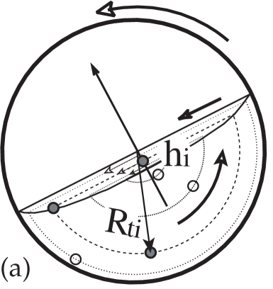
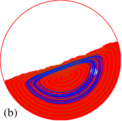
Figure 2: (a) Each depth $h_{i}$ in the flowing layer corresponds to a radial position $R_{ti}$ in the static part, (b) A 4.85 cm diameter rotating tumbler with 187 $\mu$m red small disks and a 3 mm white tracer, $d_{t}/d=$ 16. The blue curve is the tracer trajectory. The tracer stabilizes at an intermediate depth and radial position. Green thin lines are the streamlines of the small disks.

Each time $i$ the tracer passes through the vertical plane $x=0$ in the static rotating zone, the distance from the tracer center to the cylinder center $R_{ti}$ is measured. A mean position $R_{t}$ and a standard deviation are computed. Small standard deviations indicate strong localization at the same radial position from turn to turn. This corresponds to stabilization at a constant depth $h$ in the flowing layer. This also corresponds to segregation rather than to mixing since several non-interacting tracers would all stabilize at these well-defined depth and radial position. Consequently, they would regroup, i.e., segregate on this ring, exhibiting this small deviation. We choose to call the equilibrium radial position $R_{t}$ a radius of segregation, because it corresponds to the experimental segregation half-ring radius obtained with 3% of tracers (for a comparison between experiment and simulation see Fig. 1). Averaging and deviation calculation are done on one tracer during several turns for numerical data, or on several tracers at a given moment for experimental data, thus including trajectory fluctuations, but also potential tracer interactions and experimental errors.

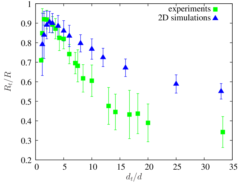
Figure 3: Relative tracer radial positions in the cylindrical tumbler versus size ratio $d_{t}/d$, for : several tracers in 3D experiments (green $\blacksquare$) FelixThomas04 and several passages of one tracer in 2D simulations (blue $\blacktriangle$). Error bars show the standard deviation.

In the simulations, a tracer with a size ratio from 1.2 to 3 is at the periphery, which corresponds to a surface position during flow. Each larger tracer nearly remains at an intermediate radial position $R_{t}$ inside the drum (Fig. 2(b)), which corresponds to an intermediate depth during flow. As $R_{t}$ decreases toward zero with increasing size ratio, we deduce that the tracer position is progressively deeper in the flowing layer. Fig. 3 represents the evolution of $R_{t}$ with the diameter ratio $d_{t}/d$ showing the reversal of the tracer position with increasing size ratio. Each standard deviation value indicates whether there is a well-defined position or a dispersed trajectory within the tumbler. In the event that several tracers are used a well-defined position leads to segregation and the dispersed trajectory leads to mixing. In the tumbler, the spatial organization passes from a spread of the instantaneous positions (for size ratio near 1) to well-defined equilibrium mean positions: at the surface (maximum of $R_{t}$ is $R-d_{t}/2$), then at intermediate depths when $R_{t}$ decreases, and toward reverse depths for the lowest values of $R_{t}$.

We compare the successive numerical positions of one tracer, and the experimental positions of several tracers, both giving a value for $R_{t}$ and a standard deviation. The agreement between experiments and simulations is good, but only qualitative, with a similar evolution of the curve. Both simulations and experiments show the reversal of either the equilibrium position or the segregation location (Fig. 3). There are differences between 3D experiments and 2D simulations: (1) In 3D experiments, the decrease of the curve $R_{t}/R$ versus $d_{t}/d$ is more rapid than in 2D simulations. (2) In 2D simulations, the asymptotic value of the curve is close to 0.55, a larger value than the asymptotic value in the 3D experiments, around $R_{t}/R=0.35$. This 2D asymptotic value will barely be reduced for larger size ratios (Fig. 4). (3) Another difference is observed regarding the maximum of the curve (surface segregation) which occurs for $d_{t}/d=$ 1.5 or 1.8 in experiments, instead of $d_{t}/d=$ 2.5 in the 2D simulations (Fig. 3). We will see that these differences are due to the 2D nature of these simulations rather than to an experiment-simulation discrepancy. A longer discussion on that point is presented with the 3D simulations.

III.1.2 Higher size ratios

To explore the asymptotic value, we need to reach larger size ratios, which would require the use of a high number of small particles in the simulations. To overcome this disadvantage several larger tracer sizes are tested ($d_{t}=3$, 4.85, 6 and 9.7 mm) in the tumbler $D=48.5$ mm, and their equilibrium positions $R_{t}$ are compared (for size ratios 25 and 40). Up to a diameter of $d_{t}=6$ mm, $R_{t}$ are almost identical. For the largest tracer ($d_{t}=9.7$ mm, whose size is to be compared with the drum diameter $D=5d_{t}$), a small discrepancy (relative error of 4%) is observed. We choose to keep the size of the tracer under $d_{t}=D/10$ to be sure that there would be no effect of the tracer size. For the particles and tumbler studied here, the thickness of the flowing layer is always larger than one tracer diameter.

A tracer diameter $d_{t}=4.85$ mm is adopted to reach large size ratios up to 60.

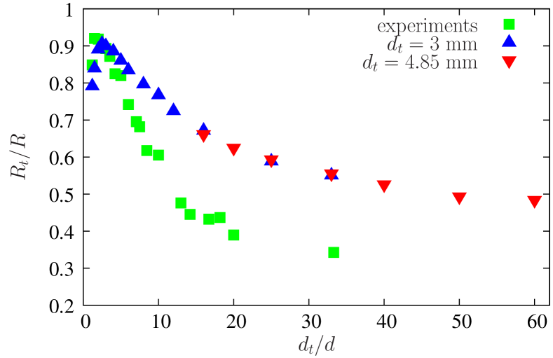
Figure 4: Relative tracer positions in the tumbler versus size ratio $d_{t}/d$, for 3D experiments with 3% of tracers FelixThomas04 and 2D simulations with 2 tracer sizes, 3 and 4.85 mm (no standard deviation here).

Fig. 4 shows the relative positions $R_{t}/R$ of the 3 mm and 4.85 mm tracers, compared to 3D experimental results. When the 2 different tracers have the same size ratio $d_{t}/d$, the resulting positions coincide. For the largest size ratios used in these 2D simulations, the radial position slowly decreases but remains close to 0.5, and does not reach the experimental value of 0.35. 2D simulation and 3D experiment asymptotic $R_{t}$ values are different. Even if there is a qualitative agreement, 3D simulations are needed for an accurate comparison.

III.2 3D rotating tumblers

III.2.1 Comparison with experiments

To obtain a quantitative agreement, 3D simulations are conducted (Fig. 5).

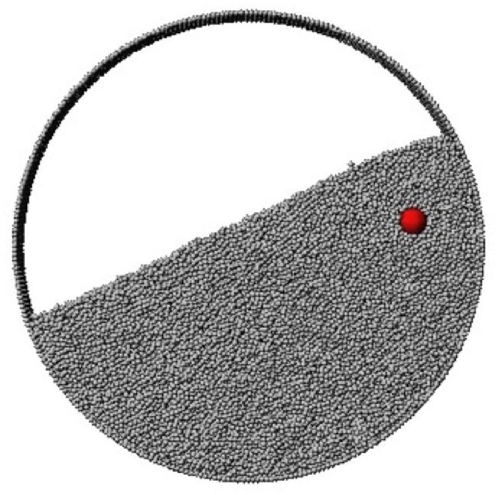
Figure 5: 3D simulation of a rotating cylinder (diameter 48.5 mm) with a 3 mm tracer in 0.5 mm small beads.

The tumbler inner diameter is equal to $D=48.5$ mm and it rotates around the $y$ axis at 15 rpm. In a first series (size ratio up to 8), the tracer diameter is set to $d_{t}=3$ mm as in experiments, then for larger size ratios (from 5 to 25) it is set to $d_{t}=4.8$ mm to reduce the number of small simulated beads. For size ratios $d_{t}/d=5$ and 8, both tracer sizes are tested. Larger tracers ($d_{t}=6$ and 9 mm) are also used respectively from size ratios 5 to 25 and 12 to 25 to check the sensitivity to the tracer size. As in 2D, no differences are observed for the 6 mm tracer, and very small discrepancies are observed for the 9 mm tracer.

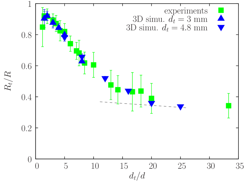
Figure 6: Relative radial positions of the tracers versus size ratio, in 3D experiments (3% of tracers) FelixThomas04 and 3D simulations (one tracer, 3 or 4.8 mm). The numerical standard deviation is very small (error bars). The dashed line is the position of a tracer touching the bottom of the flow.

The 3D numerical results show the evolution of the tracer radial position $R_{t}$ from the periphery to intermediate positions, toward the reverse position when the size ratio is increased (Fig. 6). The standard deviation is very small, indicating a strong localization on the same radial position from turn to turn. The 3D numerical radial position quantitatively matches the 3D experimental radial segregated position of several tracers. Agreement is very good, even on precise points like: 1) the slope of the curve, 2) the asymptotic value of $R_{t}/R$ for large size ratios, and 3) the diameter ratio which corresponds to the maximum of the curve. The agreement confirms our hypothesis that a few tracers locate themselves on a ring which has the same radius as the equilibrium radial position of one single tracer. The segregation of several non-interacting tracers can be seen as the regrouping at an identical position because the equilibrium radial position of each tracer depends only on its size ratio. The tracers do not interact much at this small fraction (3%), nevertheless their interaction leads to a slight increase in the standard deviation, with no observable change in the mean value. We can speak interchangeably of segregation radius or of equilibrium radial position. Moreover, as the agreement is really quantitative, we are confident in our simulation method to be used to study other systems, such as flows on rough inclines.

III.2.2 Trajectories in 3D tumbler

To gain a better understanding of the segregation phenomenon, tracer trajectories are studied in details. Fig. 7(a) shows the trajectory of a large particle with a size ratio of 4 and the streamlines of small beads in a plane $x-z$. Two phases are distinguished: first, the unsteady stage, second a stationary trajectory when the equilibrium depth is reached.

The tracer initially falls after the tumbler has been filled (vertical line), then the rotation starts with the tracer relatively close to the stagnation point. During the first, second, third passages, and the first part of the fourth passage in the flowing layer, the tracer exhibits an upward motion when compared to the small bead streamlines. It migrates towards its equilibrium position. Accordingly, in the static zone, from one passage to the next, the radial position $R_{ti}$ increases. Then, after these 4 passages, the trajectory is stationary: the tracer flows along the streamlines at each passage, and presents a nearly constant radial position $R_{ti}$ with some fluctuations from turn to turn. This confirms the experimental observation that after 3 rotations ($\simeq 6$ passages through the flowing layer for a half-filled drum) the whole segregation process is over Thomas00 . The convergence to an equilibrium depth, and consequently the segregation process, happens mainly during flow, and is not due to processes happening during the entrance into and/or the exit from the flowing layer. Here, the tracer starts from a central position, and moves upwards to reach its equilibrium depth. It could have been downwards if the tracer had been released from the surface of the flow (or periphery in the static part). An equivalent upward motion is observed for a tracer with a size ratio 8 (Fig. 7(b)), but its amplitude is smaller, as the starting position is closer to the equilibrium $R_{t}/R$ corresponding to this size ratio. A more rapid downward motion toward the same equilibrium radial position is observed when the tracer is released at the periphery, probably because of the longer distance traveled in the flowing layer.

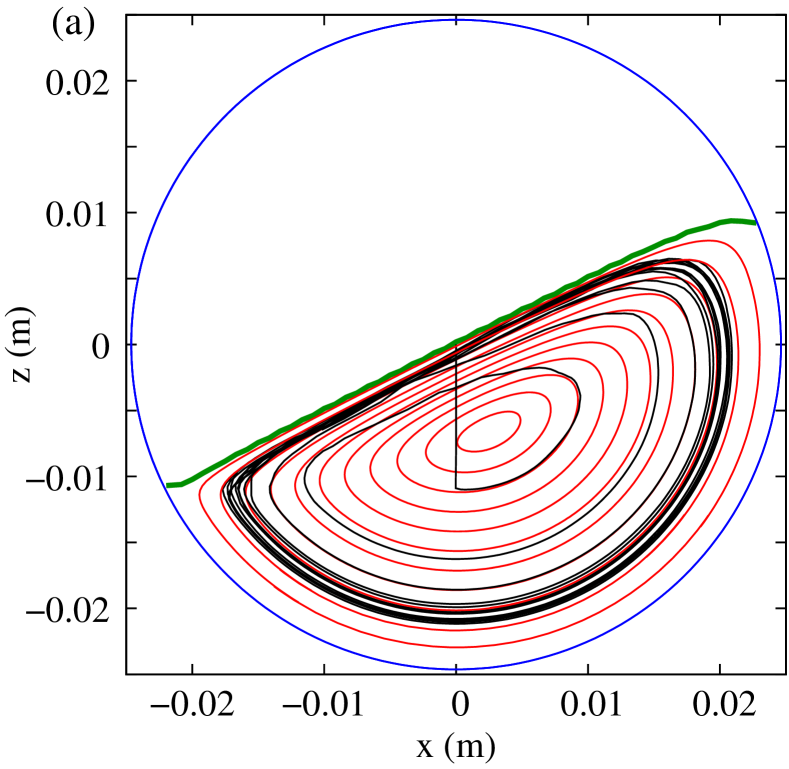
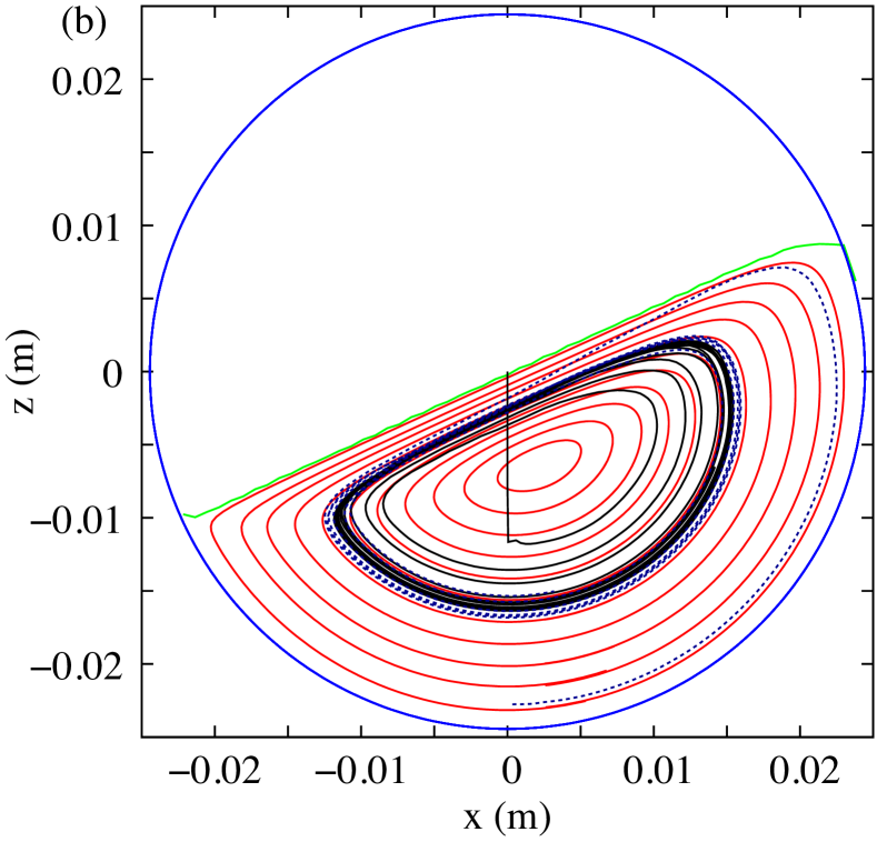
Figure 7: Trajectories of the tracer center (black curves), and small bead streamlines (red curves) ($D=48.5$ mm, $d_{t}=3$ mm). The thick green curve is the free surface. The first rotations concern the convergence, the following rotations concern the stationary phase. (a) $d_{t}/d=4$, the tracer is at the limit between surface and intermediate positions, its top touching the free surface, (b) $d_{t}/d=8$ either starting from the periphery (dashed line) or from the tumbler center (solid line), the tracer is at an intermediate position.

Once in the steady phase, the tracer trajectory and small bead streamlines are parallel in the flowing zone. There is no relative motion any longer, either up or down. Plotting a circle 3 mm on the trajectory shows that the tracer with size ratio 4 is just below the surface, and that the tracer with size ratio 8 is on a mid-height intermediate depth. Each depth in the flowing layer corresponds to one radial position in the rotating part of the tumbler. However, the tracer trajectory does not match exactly the same small bead streamline in the rotating zone and in the flowing zone. There are two small shifts between the tracer trajectory and the small bead streamlines when going in and out of the flowing layer. At the entrance (Fig. 7(b)), the tracer starts to move after the small beads on the same streamline (despite the shift occurring at the previous exit), probably because its bottom is still surrounded with non-moving small beads. At the exit of the flow, the tracer stops before the small beads on its corresponding streamline because its lower part is touching the static curved bottom (note that these entrance and exit shifts are enhanced in 2D (Fig. 2)). In conclusion, these shifts are not responsible for the segregation from turn to turn. But they exist, they probably vary with $R_{t}$ and might be one cause of the discrepancy between 2D and 3D. For that reason, it is not possible to easily deduce the flowing depth positions from both data of small particle streamlines and $R_{t}/R$. Nevertheless, the shifts are very small and the $R_{t}/R$ variation mainly reflects a variation in depth within the flowing layer.

A more accurate examination of the trajectory reveals that the entrance in the flow induces a starting point slightly above the equilibrium depth that the tracer will reach (Fig. 7(a)). Each time it passes through the flowing layer, the tracer exhibits a tiny descent towards its equilibrium depth, then remains at a constant depth to the end of the flow, parallel to streamlines. The length at which the constant depth is reached seems to decrease with the tracer size ratio, approximately at mid-length for ratio 4, almost immediately for ratio 8 (Fig. 7). Segregation is so fast that slight destabilization can be rebalanced in less than one passage in the flow.

In conclusion, the study of trajectory in the 3D cylindrical tumbler shows that the process responsible for the segregated radial positions of tracers is a vertical migration and stabilization of the tracer at various depths, occurring during flow. We then expect a similar phenomenon to happen during flow on an incline.

III.2.3 Radial position and depth within the flowing layer

One may wonder how the different values of $R_{t}/R$ should be interpreted in terms of equilibrium depth within the flowing layer of the tumbler, to anticipate conclusions across the tumbler study and the following incline study. In particular, the question arises whether the asymptotic small values of $R_{t}/R$ do correspond or not to a reverse segregation within the flow. A tracer touching the bottom of the flow undergoes a small decrease in $R_{t}/R$ with the size ratio, because with our protocol ($d$ decreasing) the thickness of the flowing layer slightly decreases FelixFalk07 . Numerical thickness measurements, added with a tracer radius to obtain the tracer center position, are shown as a dashed line on Fig. 6: it would correspond to reverse positions, turning around the stagnation point. We deduce that size ratios 20 and 25 are in reverse position, and that the small decrease between them is explained by the choice of the protocol.

In addition, in some simulations, we measure the depth of the tracer directly on its trajectory. For a ratio 8, (Fig. 7(b)) the tracer is at an intermediate depth. For the largest size ratios (for example, ratio 20), the tracer is just touching the bottom of the flowing layer, i.e., the bottom of the tracer passes where the streamlines are reduced to the stagnation point, which is nowhere else than the middle point of the bottom. But this method is not precise: it is difficult to define the bottom of a flowing layer near the tracer. The bottom of the flowing layer is defined by an averaging of small bead streamlines. The tracer passage has almost no effect on the averaging, although it probably deforms locally and during a short time the granular material below and around it when it passes “at the bottom”. Consequently, the bottom of the averaged flowing layer may not be the same as the local bottom of the flow around the tracer. Nevertheless, we choose to call the positions of these tracers with the largest ratios ”reversed”, keeping in mind that this is somehow arbitrary. In fact, denser tracers may be found at lower $R_{t}$ than the asymptotic value, probably because they more strongly deform the bottom FelixThomas04 . With that choice, all the asymptotic $R_{t}/R$ positions correspond to a tracer in a reverse bottom position within the flow. In conclusion, reverse depth is reached for tracers with a size ratio$\geqslant$ 20 in 3D. The same measurements on trajectories are made in 2D: tracers are found at intermediate depth for size ratio 10, 16 and 20, and in reverse position for size ratios above 40. The reverse position can be reached both in 2D and 3D, but for greater size ratios in 2D.

III.2.4 Differences between 2D and 3D tumblers

Compared with 3D results, 2D results are shifted, as if the size ratio had a reduced effect: the maximum of the $R_{t}/R$ curve occurs for a higher size ratio, the dependency is smaller, and the asymptotic value is higher (Figs. 6 and 4). We first check that the difference between 2D and 3D is not due to a variation of the thickness of the flowing zone. Indeed, the thicknesses have been measured nearly identical for a given small bead size in 2D and 3D tumblers. Secondly, for a given size ratio ($d_{t}/d=$20) we compare the depth of each tracer on its trajectory within the flow: in 3D, the tracer is touching the bottom, while in 2D, 6 small beads are under the tracer (this flow thickness is 25$d$). The shift between 2D and 3D $R_{t}/R$ curves does correspond to a real difference in depth positions within the flowing layer.

Nevertheless, a radial position difference in 2D and 3D can also be seen for tracers at the same depth. For example, for the asymptotic values, the largest tracers in 2D (size ratios above 40) and in 3D (size ratios 20 and 25) are all measured touching the bottom of the flowing layer. The size of the tracer is fixed ($d_{t}=4.8$ mm or 4.85) and the thickness of the flowing layer is almost unchanged for these small bead sizes $d$ (a slight decrease indicated by the dashed line in Fig. 6). Nevertheless, there is a gap between the 2D and 3D values of $R_{t}/R$ corresponding to these identical reverse depths (Fig. 4). Note that to take into account the slight variation in the flowing layer thickness with the small bead size, one can simply extrapolate $R_{t}/R$ values in 3D up to 40 (Fig. 4), and compare radial positions exactly at the same flowing thickness: the conclusion is unchanged.

Considering tracers at a same depth, the $R_{t}/R$ difference is mainly due to the larger trajectory fluctuations in 2D which shift $R_{t}$ to larger values in 2D when approaching the bottom (and to smaller values when nearing the surface). It is also due to a difference in the entrance and exit of the flowing layer, which gives smaller $R_{t}$ values in 2D. This latter effect pushes in the opposite direction, but is small compared to the former one.

We have seen that there is a difference between the 2D and 3D equilibrium depths within the flowing layer all along their evolution with the size ratio. To understand the cause of this difference, one should compare the effective densities of the medium made up of small particles. If we note $\rho$ the density of the small (or large) particles, the effective density of the granular medium made up of small particles is equal to $c\,\rho$, where $c$ is the compacity. A large tracer is denser than a sphere/disk of the same diameter filled with a random close packing of small particles. In 2D, such a packing gives a compacity close to $c_{2d}\simeq 0.8$, while in 3D, $c_{3d}\simeq 0.6$. Thus, the density ratio between the tracer and the medium is larger in 3D than in 2D, leading to deeper intermediate segregation and advanced reverse segregation. This result was confirmed using tracers of decreasing densities FelixThomas04 . For tracers less dense than a random packing of small particles, only surface segregation of the tracer is observed.

Even if the names and limits of the equilibrium depths are arguable, there are similarities but also discrepancies between 2D and 3D cases. In 3D, the evolution of the position shows a shift of the curve maximum toward smaller size ratios and a stronger dependency with size ratio. If the enhancement of the effect of the size ratio is due to the compacity around 0.6 (in 3D) instead of 0.8 (in 2D), we expect that it will always be present in all types of flow. Thus, care should be taken when extrapolating these 2D studies to the 3D case.

IV Rough incline

The experimental study of granular segregation occurring during flow down an incline is a difficult task to achieve in wide and thick channels (3D). Indeed, in our previous experiments Thomas00 only the surface of the flow was visible. A fraction of 10% of large particles was used. For large size ratios ($d_{t}/d\geqslant 6$), no tracers were visible at the surface during flow, although for $d_{t}/d\leqslant 3$, large particles were at the surface. The volume of the deposit could be accessed after the flow had stopped due to a slope change or a vertical end wall. But the aggradation of the deposit may have modified the particle depths. Size ratio had been varied and the segregation pattern in the deposit changed according to the size ratio: for small size ratios, the large particles covered the surface of the deposit, while for larger size ratios, the large particles were found inside the deposit. The individual positions were moderately spread inside the deposit. Nevertheless, their mean position was at an intermediate depth, which was deeper and deeper with increasing size ratios. Because of this spread and because of the aggradation, it was not possible to conclude on whether these tracers were located at a well-defined intermediate depth during flow (corresponding to an intermediate segregation). Simulations will allow measurements during flow, in an established steady-state regime, with a single tracer.

The main advantage of the incline geometry is that the measurements of tracer depths within the flows are direct, while measurements of radial positions in the tumbler involve entrance in the flowing layer, acceleration and exit from the flowing layer. Moreover, for a solid rough incline, the bottom depth can be accurately determined, which is not the case in a partially filled tumbler where flow passes on loose granular matter having a curved bottom shape. Another difference is that the flow thickness in the tumbler is mainly imposed by the dimensions (tumbler diameter and small particle size). For the chosen protocol (decreasing small bead size), this layer thickness decreases with the size ratio (around $8d$ for $d_{t}/d=2$; $21d$ for $d_{t}/d=10$; 34$d$ for $d_{t}/d=25$, respectively: 4, 2.1 and 1.4$d_{t}$), while for confined flows in an inclined channel the thickness of the flow can be varied independently. In the present study, the smallest thickness chosen is comparable to those encountered in non-confined flows on an incline (around $10d$) FelixThomas04e , and, for this reason, the results on such thin flows are not without interest. The thickness will be increased ($37d$), to explore thickness effects, and will reach the values for experimental channel flows, for comparison Thomas00 .

As experimental results were obtained without following any protocol, we choose to keep the small bead size constant ($d=6$ mm), and vary the tracer size ($d_{t}$). Indeed, decreasing the small bead size would have resulted in increased flow velocity and increased calculation time for a constant flow thickness. Nevertheless, we may expect some deviations between experimental and numerical results if the tracer becomes too large compared with the flow thickness.

IV.1 2D simulations of flows on an incline

IV.1.1 Intermediate segregation

Even though quantitative agreement cannot be taken for granted, we first perform 2D simulations. The simulation domains are 160$d$ long, or 300$d$ long for the larger tracers ($d_{t}/d\geqslant 8$). Fig. 8 shows a 48 mm diameter tracer (disk) in a granular flow made up of 6 mm small disks flowing down an incline. The plane slope is 20^∘ and the thickness of the flow $h_{max}$ is around 36 cm.

Figure 8: A 2D granular flow down a rough incline with 6 mm small disks and a 48 mm large tracer, moving from left to right. The slope angle is 20^∘, the flow thickness is 36 cm.

The tracer with this size ratio ($d_{t}/d=8$) is not far from the free “1D surface” but remains below it, fluctuating around an intermediate depth. This does not correspond to the behavior of a large particle during the classical granular surface segregation of large particles, but to that of a particle flowing inside the bed, at an equilibrium intermediate depth: this would lead to intermediate segregation if several non-interacting tracers of the same size were present.

Figure 9: Trajectories of the center of 3 tracers versus time. The horizontal dashed line is the free 2D “surface”. Thick circles show the sizes of the three tracers.

Figure 9 shows the depth $z(t)$ of each tracer center for three different tracer sizes versus time $t$ (each simulation involving one single tracer). For each tracer size, several initial positions at the bottom or at the surface are tested, but only one is plotted here. The steady state tracer depth $h$ does not depend on the initial location ($h$ is the mean of $z(t)$, the initial convergence time being removed). For the size ratio $d_{t}/d=8$, the tracer almost never reaches the free “surface” and stays at an intermediate depth. It is the noisiest trajectory. At intermediate depths, the trajectory is not stabilized by the existence of the free “surface” or the bottom nearby. For the size ratio $d_{t}/d=20$, the tracer reaches an equilibrium depth located near the center of the flow with a layer of around 22 small particles below it. The $d_{t}/d=3$ tracer, initially placed at the bottom, reaches the surface, as in a surface segregation phenomenon. Stationary positions are reached after horizontal displacements of 10000$d$, 25000$d$ and 30000$d$ for tracers of size ratio 20, 8, and 3 respectively. The distance is mainly due to the gap between the initial vertical position of each tracer and its corresponding stationary position. Large values are explained by the use of a thick flow (60$d$), and by the poor efficiency of the 2D segregation.

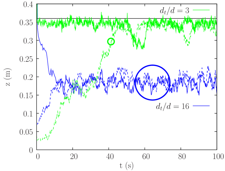
Figure 10: Trajectories of a tracer released at the top (solid lines) and the bottom (dashed lines) of the flow. Both trajectories converge to the same equilibrium depth (intermediate for $d_{t}/d=16$, at surface for $d_{t}/d=3$). Circles show the tracer sizes. The horizontal black line is the mean position of the free 2D “surface”.

For a size ratio of 16, trajectories starting from the top and from the bottom reach the same equilibrium depth in about 12-15 seconds (around 4000-5000$d$) (Fig. 10). The initial gap to stationary position is the main parameter which determines the time or distance to travel along. It takes a longer time (and distance), around 55 seconds, (22000$d$) to the tracer with size ratio 3 starting from the bottom to reach the surface: it has to move across the whole flow thickness, on a trajectory showing larger fluctuations.

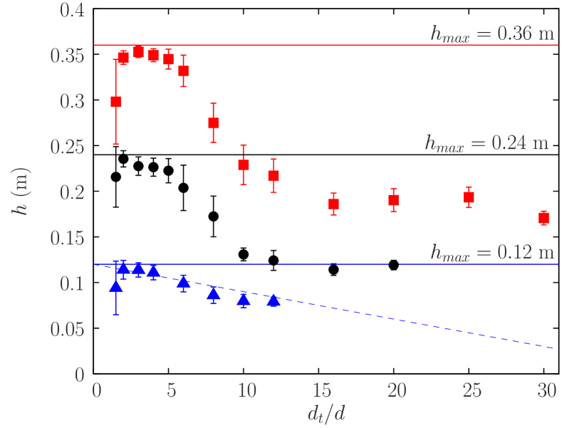
Figure 11: Equilibrium depths of the tracer center in a flow down a 2D incline versus size ratio, for 3 flow thicknesses: (blue $\blacktriangle$) 0.12 m, (black $\bullet$) 0.24 m, (red $\blacksquare$) 0.36 m. Error bars show the standard deviation. Horizontal lines show the free “surfaces”. The oblique dashed line corresponds to the position of a tracer whose top is at the surface of the thinnest flow.

In order to study where the tracer stabilizes, the mean depth of one tracer in the stationary regime $h$ is reported for several size ratios $d_{t}/d$ (with $d$ = 6 mm) and for several thicknesses of the flow $h_{max}$ (Fig. 11). $h$ is calculated from the flow bottom to the tracer center. Moderately large tracers ($2\leqslant d_{t}/d\leqslant 6$) are found at or near the surface, and $h$ is maximum for a size ratio between 2 and 3. For these low size ratios, the values of $h$ seem related to the distance to the free “surface”, independently of the thickness of the flow, showing the same curve shape relatively to the flow surface. For larger size ratios ($d_{t}/d\geqslant 7$), the tracer position gets deeper and with increasing size ratios. It is compatible with the $R_{t}/R$ vs $d_{t}/d$ decrease in the tumbler. The $h$ asymptotic value for very large size ratios is close to $h_{max}/2$, and thus scales with the thickness of the flow (Fig. 12).

The interesting result is that there are some tracers which stabilize at intermediate depths inside the flow. This shows the occurrence of intermediate segregation in a 2D flow on a rough incline, at least for non-interacting tracers. We can assume that small fractions of large disks would undergo intermediate segregation for these size ratios. The small standard deviations represented as error bars indicate that each tracer does not explore the whole thickness of the flow, but remains at an intermediate well-defined depth, with little randomness in its trajectory. These small fluctuations would correspond to a small standard deviation in the segregation of several non-interacting tracers.

Note that for thin flows, tracers with size ratios above 10 are very large compared to the flow thickness and they are close to appearing at the “surface”, although they interact with the bottom at the same time. The oblique dashed line shows the position of a tracer such that its top is flush with the free “surface” of the flow (Fig. 11). It defines a boundary between surface and intermediate positions (for small size ratios, here around 5), and also shows a reasonable size limit for a tracer in such thin flow (here, $d_{t}/d=12$).

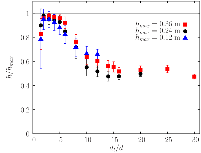
Figure 12: Relative equilibrium depths of the tracer center in the 2D flow versus size ratio, for three flow thicknesses: (blue $\blacktriangle$) 0.12 m, (black $\bullet$) 0.24 m, (red $\blacksquare$) 0.36 m.

If the vertical position is renormalized by the thickness of the flow (Fig. 12), the three previous curves collapse reasonably well. Note also that for $1.5\leqslant d_{t}/d\leqslant 6$, rescaling like $h_{max}-h$ is a better choice as curves match well in their upper part, but they will no longer collapse for large size ratios. Thus the behavior in a 2D flow shows two regimes: a first one (tracer near or at the surface) where the equilibrium position depends on the distance to the “surface”, independently of $h_{max}$ value, and a second one where the equilibrium depth is intermediate and tends towards $h_{max}/2$, and thus scales with the flow thickness.

The positions $h$ show that only surface and intermediate depths are obtained in 2D granular flows on an incline. We conclude that reverse segregation is not obtained in 2D, at least in this parameter range. The large tracer does not reach positions below mid-height of the flow, even for very large size ratios. For the thinnest flow, the depths are compatible both with a reverse and an intermediate pattern, considering the small number of small particles below the tracer, but for thicker flows both types of depths can be differentiated. Equilibrium positions end up really at mid-flow for the largest ratios. There are 14 small particles below the largest tracer in the thickest flow, significantly above a reverse position.

Since in tumblers the dependency of the position $R_{t}$ on $d_{t}/d$ is stronger in 3D than in 2D, we expect different results for a 3D incline flow. Another point worth noting is that the dependency of the position ($h$ or $R_{t}/R$) on $d_{t}/d$ is also greater for a 2D incline than for a 2D tumbler and consequently, the asymptotic value is approached for smaller size ratios on an incline than in a tumbler flow.

IV.1.2 Slope angle

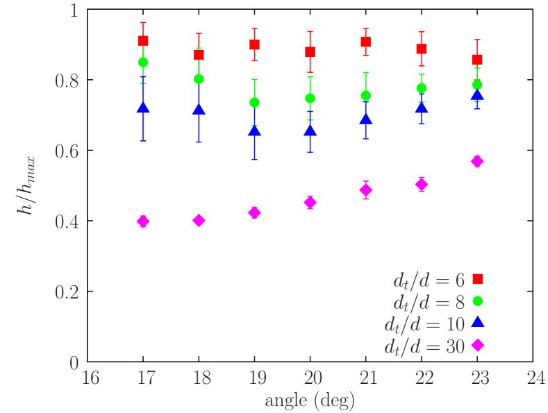
Figure 13: Relative equilibrium depths of the tracers in a 2D flow versus slope angle ($\theta=17$ to 23^∘) for 4 size ratios: $d_{t}/d=6$, 8, 10 and 30. The flow thickness is $h_{max}=$ 36 cm.

In a granular flow down an incline, the easiest way to increase the shear rate, without changing the thickness of the flow, is to increase the slope. Fig. 13 shows the relative position of four tracers, with size ratios $d_{t}/d=6$, 8, 10 and 30, for several angles of the plane. Even if small evolutions are measurable, the relative vertical position of tracers ($d_{t}/d\leqslant 10$) is almost unchanged for a slope change from 17 to 23^∘ although this change induces an increase in the mean velocity of the flow, and thus in the shear rate, by a factor of 4. In the case of a $d_{t}/d=30$ tracer, a slight monotonic increase in the tracer depth with the slope is observed. For size ratio 10, the same increase is obtained but only for slopes larger than 20^∘.

IV.2 3D flows on an incline

A series of simulations is conducted on the 3D incline, first in a thin flow, then in thicker flows. Even though very large size ratios are not reachable with our computational facilities, this captures most of the phenomena and allows a comparison with the 2D case and with previous experiments in a 3D channel.

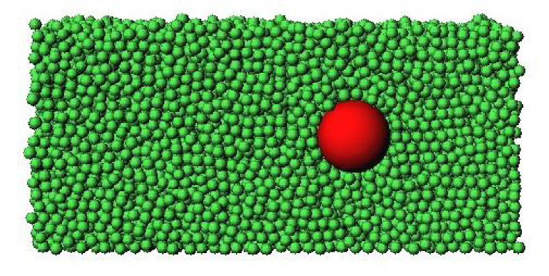
Figure 14: A 3D incline granular flow, with a tracer ($d_{t}/d=6$), moving from left to right (slope is 23^∘, $h_{max}=0.112$ m). Side beads have been removed to show the tracer.

IV.2.1 Equilibrium positions

Figure 14 shows a 3D flow, with a tracer having a size ratio $d_{t}/d=6$ (small beads are $d=6$ mm). The horizontal dimensions of the simulation domain are 20$d$ $\times$ 20$d$ (0.12 m $\times$ 0.12 m) or (40$d$ $\times$ 40$d$) for the largest size ratios. Both domain sizes are used for several size ratios to be sure that the simulated domain is large enough (Fig. 15). The flow thickness ($h_{max}=0.112$ m $\simeq$ 18$d$) corresponds to a relatively thin flow, comparable to the flows encountered in our 3D tumbler for size ratios around 8. The tilt angle is 23^∘.

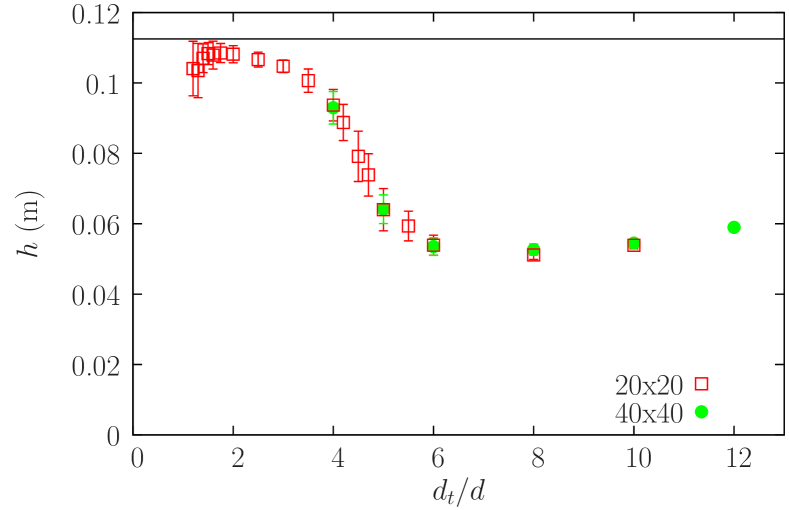
Figure 15: Equilibrium depths of the tracer center in the 3D flow down an incline versus size ratio $d_{t}/d$. Error bars show the standard deviation. The horizontal line is the free surface ($h_{max}=0.112$ m, the slope is 23^∘). Two numerical domain sizes are used: 20$d$ $\times$ 20$d$ (red $\square$) and 40$d$ $\times$ 40$d$ (green $\bullet$).

For each size ratio (from 1.2 to 12), the large tracer depth $z(t)$ evolves rapidly during flow (see below Figs. 16 and 17) to stabilize finally at a constant depth $h$. Some tracers have been initially placed at the bottom of the flow, and some at the surface without any final difference. Once in steady state, trajectory fluctuations are small and give small standard deviation associated with each $h$.

The equilibrium depth $h$ depends on the size ratio between tracer and small beads. Fig. 15 plots the tracer depths (from 7.2 to 72  mm in size) for size ratios ranging from $d_{t}/d=1.2$ to 12. For moderately large size ratios (below 4), $h$ is near or at the surface, in accordance with the surface segregation of large beads. As in the 3D rotating tumbler, the maximum of the curve (i.e., tracer at the free surface) is obtained for size ratios between 1.5 and 1.8 (Fig. 15). For size ratios approximately between 4 and 6, the tracer reaches an equilibrium depth inside the flow, suggesting the occurrence of intermediate segregation in 3D flow down an incline, for non-interacting tracers. For larger size ratios, $d_{t}/d>6$, the equilibrium depths reach a saturation value near the bottom, in a reverse position. We note that the equilibrium positions are independent of the size of the simulation domain. The slight increase of the curve for the largest size ratios (10 and 12) is due to the increase in the tracer size itself, showing that the tracer is in strong interaction with the bottom. There are only about 4 small beads below the tracer. The three types of equilibrium positions (surface-intermediate-reverse) are thus found in this thin 3D flow, suggesting that the three segregation patterns would exist for a small fraction of non-interacting tracers.

Comparing 2D and 3D cases (Figs. 12 and 15 respectively), the overall behavior is the same but some differences are present. In the 3D case, the equilibrium depth decreases more rapidly and reaches a smaller saturation value earlier, at a size ratio close to $d_{t}/d=6$ in 3D, instead of $d_{t}/d=$ 10 or 15 in 2D. We also note that the standard deviations are much smaller in 3D.

IV.2.2 Thickness of the flow

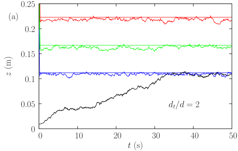
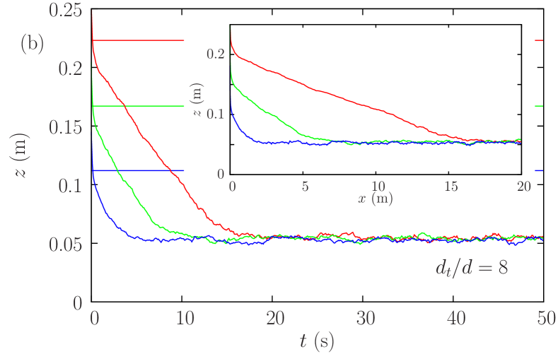
Figure 16: Trajectories of tracers in the 3D incline flow (slope is 23^∘) for 3 flow thicknesses $h_{max}=0.112$ m, 0.167 m and 0.223 m and for 2 size ratios: (a) $d_{t}/d=2$ and (b) $d_{t}/d=8$, insert: trajectories in $x$ coordinate.

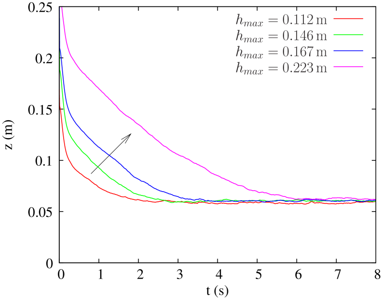
Figure 17: Trajectory of a tracer center ($d_{t}/d=12$), initially placed at the surface, in a 3D flow, for 4 flow thicknesses (slope is 23^∘). The arrow indicates increasing thicknesses.

Figure 16 shows the trajectories for the first 50 seconds of two tracers, $d_{t}/d=2$ and 8, immersed in granular flows having three different thicknesses. The horizontal lines show the positions of the free surfaces of the flows: $h_{max}=0.112$ m, 0.167 m and 0.223 m. For the three thicknesses, the tracer with a size ratio of 2 remains at or goes to the surface of the flow showing the same final position as in a surface segregation process (only the case of the thinnest flow is shown for the ratio 2 tracer placed at the bottom). When crossing the whole thickness, the convergence is longer for this small size ratio ($d_{t}/d=2$) than for a larger one ($d_{t}/d=8$), and the trajectory presents more fluctuations. The large tracer ($d_{t}/d=8$) sinks to reach a depth near the bottom of the flow. Its stationary depth is close to 0.05 m, independently of the thickness of the flow. As the tracer radius is $r_{t}=0.024$ m, it does not touch the rough inclined plane made up of small glued beads, but about 4 small beads remain between the tracer and the plane. We consider this position close enough to the bottom to be called “reverse”.

When using a $t-z$ representation, parallel trajectories on Fig. 16(b) show that the sinking velocity is constant ($v_{sink}=-0.0105$m/s). For a given size ratio, the time of convergence is mainly related to the thickness of material to travel through. A constant sinking velocity is an interesting feature since it can be used in theoretical models to describe granular segregation. From an experimental point of view, an $x-z$ representation (Fig. 16(b) insert) is more interesting since it gives the incline length required for an experiment. For a size ratio of $d_{t}/d=8$, changing the thickness of the flow from $h_{max}=19d$ to 37$d$, decreases the slope of the trajectories (compared to the rough incline) and increases the horizontal settling distance from $\simeq 400d$ to $\simeq 2500d$. This distance increase comes from the flow thickness increase but also from the induced increase of the mean velocity which is about a factor 3 here. In the case of a larger tracer $d_{t}/d=12$ (Fig. 17), the sinking is more rapid ($v_{sink}=-0.021$m/s), and the slope of the trajectories also decreases with the increase in thickness (not represented). Consequently, the settling distance increases from $\simeq 200d$ to $\simeq 1200d$, for $h_{max}=0.112$ and 0.233 m respectively. For a downward motion, convergence is more rapid for high size ratios (comparing Figs. 16(b), 17 and 23). Downward forces acting on tracers are stronger when tracers are larger, and consequently heavier.

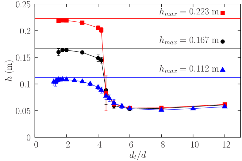
Figure 18: Equilibrium depths of tracers versus size ratio in the 3D flow for 3 thicknesses: (blue $\blacktriangle$) 0.112 m, (black $\bullet$) 0.167 m, (red $\blacksquare$) 0.223 m. Error bars show the standard deviation.

Figure 18 shows the equilibrium depth $h$ for a large tracer for three different thicknesses $h_{max}$. For size ratios up to 4, the large tracer remains at or near the surface, independently of $h_{max}$. For size ratios larger than 5, the tracer sinks close to the bottom of the flow, and $h$ is independent of $h_{max}$ (as in Figs. 16(b) and 17). The slight increase with the tracer size shows the strong interaction with the bottom when in reverse position. For the two thickest flows, a sharp transition between the surface position range and the reverse position range appears for size ratios $d_{t}/d$ between 4.2 and 4.5, while a relatively progressive variation is observed for the thinnest flow. The tracer depth $h$ depends on the flow thickness only during the transition. Both parts of the curves, $h-h_{max}$ for small (below 4) or $h$ for large size (above 5.5) ratios are independent of $h_{max}$.

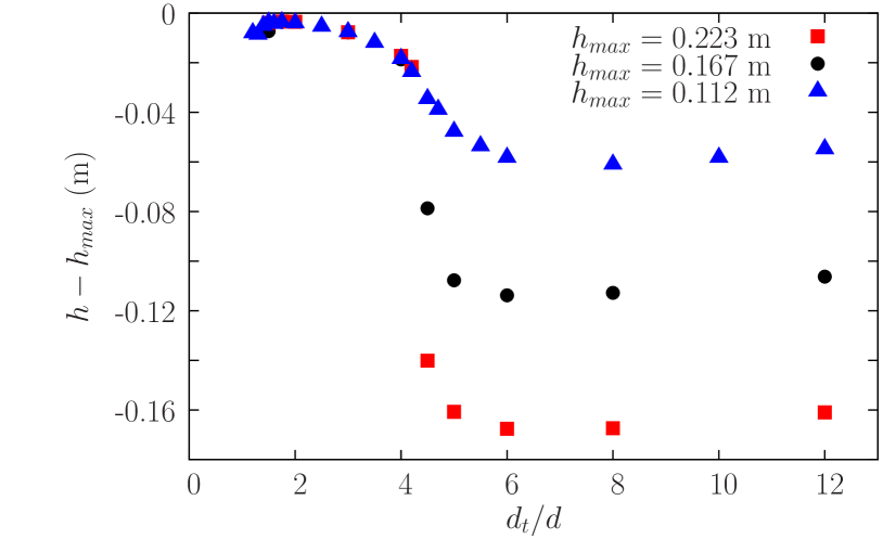
Figure 19: Equilibrium distances from the tracers to the surface $h-h_{max}$, in the 3D flow on an incline for 3 thicknesses: (blue $\blacktriangle$) 0.112 m, (black $\bullet$) 0.167 m, (red $\blacksquare$) 0.223 m.

Plotting $h$ (Fig. 18) shows that the distance to the bottom controls the equilibrium position for very large tracers, independently of the thickness of the flow. In the same way, plotting $h-h_{max}$ (Fig. 19) shows that the distance to the surface is independent of the flow thickness for moderately large tracers ($1.5\leqslant d_{t}/d\leqslant 4.2$), when positions near surface are reached. It seems that two independent phenomena, one influenced by the presence of the surface and one by the bottom, determine the equilibrium of the tracer in each case. For a thin flow, the free surface and the bottom are close enough so that the two phenomena interact, and the result is a progressive transition between the two influences, creating a larger range of intermediate segregation positions. In the case of a thick flow, both influences are almost separated and could be studied independently.

It could be tempting to associate the three zones coming from these curves (Figs. 18 and 19) with the three types of equilibrium positions: surface, intermediate and reverse (or the three segregation types). But they do not exactly match. For example, tracers just below the surface (as for a ratio 3.5) are not visible at the surface, whatever the flow thickness is: they should be considered in intermediate position. Symmetrically, the tracer with a size ratio 5 is floating above the larger ones, and is in intermediate position. As for the largest tracers ($d_{t}/d\geqslant 8$), which show a slight increase in their center depth due to the increase in their size, they are in strong interaction with the bottom plane and are thus in reverse position. The separation into three types of equilibrium depths (surface-intermediate-reverse) is convenient but may not be representative of the phenomena happening in the granular matter. Only two mechanisms may be the cause for equilibrium depths: one due to the influence of the surface and one due to the influence of the bottom. Their potential combination appears or does not appear at around mi-height of the flow, depending on the flow thickness. Nevertheless, in the present study we keep the separation in the three types (surface-intermediate-reverse) that correspond to particular positions of the tracers (and not to mechanisms). In this view, we have to split the surface zone of the $h$ curve in two layers: one layer with surface positions (visible tracers), and one layer with intermediate depths. In the same way, we split the bottom zone of the $h$ curve in two layers: a second layer with intermediate depths and one layer with reverse depths (Fig 20). In this view, thick flows have two intermediate depth layers which are separated by an empty central zone where there is no equilibrium depth for a tracer. Thin flows have their two intermediate depth layers continuously connected, forming a “thick” central layer of intermediate equilibrium depths.

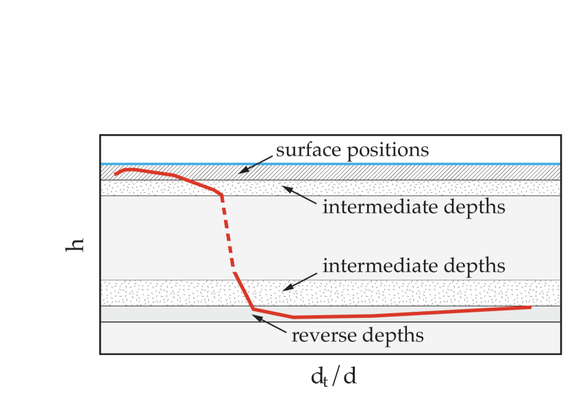
Figure 20: The upper part of the $h$ curve defines two layers, with surface and intermediate equilibrium depths, and the lower part, two layers, with intermediate and reverse equilibrium depths (red $h$ curve from Fig. 18). In a thick flow (drawn here), there are no equilibrium depths in a layer around mid-height. The bottom is never reached, partly due to the tracer size ($h\geqslant d_{t}/2$) and partly due to the presence of some small beads (around 4) under the tracer.

IV.2.3 Comparison between the 2D and 3D flows on an incline

The main difference between 2D and 3D is the equilibrium depth of very large tracers (Figs. 11 and 18). The large tracers sink near the bottom, exhibiting a reverse position in the 3D case while they locate themselves at intermediate depths in 2D, near mid-height of the flow. For $h_{max}=0.112$ in 3D, the asymptotic equilibrium depth is also close to $h_{max}/2$ (Fig. 15), but this is just a coincidence: other flows with different thicknesses show the same constant asymptotic value. The fact that the stabilization of a large tracer in 2D is $h_{max}$ dependent, while it is independent of $h_{max}$ in 3D, shows that 2D and 3D segregations of a few non-interacting large tracers may be different processes. Moreover, the transition between the surface and the deepest positions is steeper in 3D than in 2D (see Figs. 12 and 18). The transition occurs between size ratios $d_{t}/d=4$ and 6 in 3D, while in 2D the whole transition occurs between $d_{t}/d=5$ and 15. This stronger dependency in the 3D case is also observed in the tumbler. Moreover, the maximum does not occur for exactly the same size ratio in 2D and 3D. Nevertheless, similar behaviors are also noticed: for small size ratios in 2D and 3D the tracers positions are both related to the distance to the surface, independently of the $h_{max}$ value. As for the tumbler system, the 2D incline case should not be carelessly extrapolated in 3D: evolutions with the size ratio are different, even though some strong similarities are observed. These differences are probably linked to the compacity difference between 2D and 3D.

IV.2.4 Comparison between tumbler and incline

On an incline, granular matter flows on a solid rough surface whereas in tumblers, it flows on loose curved granular material. The comparison of the equilibrium position ($h$ or $R_{t}/R$) versus $d_{t}/d$ in both types of flows (incline or tumbler) gives information on the influence of the structure of the flow. Fig. 21 shows normalized depth in the incline flow $h^{*}$ and radial positions $R_{t}/R$ in the tumbler at the same scale. We choose to adjust the minimal and maximal positions of $h$ to the asymptotic and maximum values of $R_{t}/R$, which corresponds to bottom and surface tracer position, respectively, within the tumbler flowing layer. The curves match relatively well for $d_{t}/d\leqslant 3.5$, indicating that for these small size ratios the process is mainly controlled by surface phenomena, which are quite insensitive to the substratum. For larger ratios $d_{t}/d\geqslant 4$, curves shift with a stronger dependency in the case of rough inclines. The difference may come from the substratum. As the conclusions drawn from Figs. 18 and 19, these data suggest that the equilibrium at a given depth comes from one phenomenon influenced by the surface, or/and one influenced by the bottom.

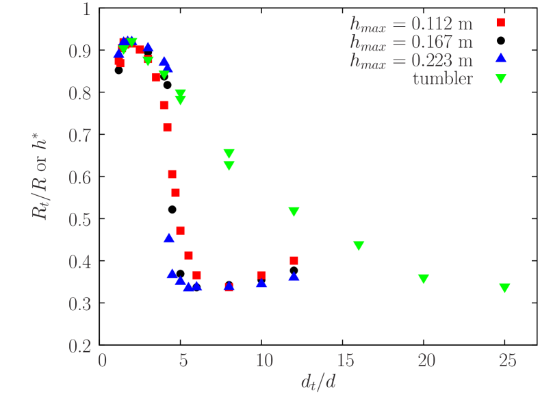
Figure 21: Equilibrium positions of the tracer versus size ratio, in the 3D tumbler (green $\blacktriangledown$) and equivalent rescaled (see text) positions in the 3D incline flow, for 3 different thicknesses.

Note that for 3D inclines, the tracer vertical position increases for size ratio starting from 1, reaches a maximum for size ratios between 1.5 and 1.8, and decreases for larger values. For 3D tumblers, the maximum is obtained for size ratios between 1.5 and 1.8 in experiments, and between 1.5 and 2 in simulations. These non-monotonic variations are analogous to those observed experimentally in an annular shear cell where the segregation time and the segregation rate both present an extremum for a size ratio of 1.6 GolickDaniels14 . This is also related to the variation of the segregation Péclet number, defined as a segregation rate on a diffusive remixing, which shows a slight maximum at 1.7 ThorntonWeinhart12 , or the variation of the force acting on a tracer in 2D, which shows a maximum at 2 Guillard16 .

IV.2.5 Slope angle

Several simulations are done for different slope angles of the plane. For thin flows, positions $h$ for tracers with small and large size ratios show no dependency on the slope, i.e., on the velocity of the flow (Fig. 22(a)). On the contrary, when getting close to the transition between surface and reverse depths (size ratio between 4 and 6), $h$ depends on the slope. The greater the angle, the deeper the tracer stabilizes. This can be interpreted by the fact that the flow being more rapid, it loses cohesion and is less able to carry large and consequently heavy tracer.

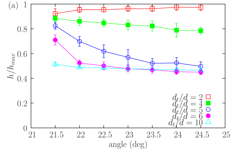
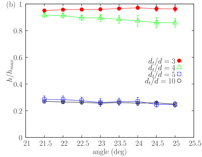
Figure 22: Equilibrium depths of tracers in a 3D flow versus slope (size ratios $d_{t}/d$ from 2 to 10). Flow thickness $h_{max}$= (a) 0.112 m (b) 0.223 m. Error bars show the standard deviation.

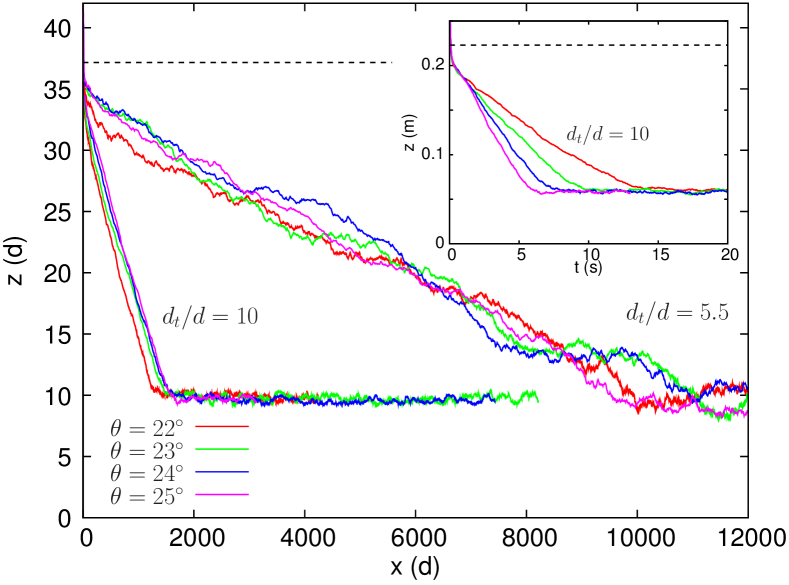
Figure 23: Tracer trajectories (x-z plane) measured in small bead diameters. $d_{t}/d=10$, $h_{max}=0.223$ m (37$d$) and slope angles 22 to 25^∘. Dashed lines show the free surface. A set of noisier trajectories are plotted for comparison (size ratio $d_{t}/d=5.5$). Insert: time evolution of the tracer depth (z-t).

In the case of a thicker flow, the equilibrium depth of the tracer shows almost no dependency on the slope (Fig. 22(b)). But no size ratios between $d_{t}/d=4$ and 5 are presented here: they do not present the usual rapid convergence to an equilibrium depth. Further investigations are needed (ongoing study on ThomasDOrtona18 ).

The time evolution of a tracer depth $z$ plotted for different angles (22 to 25^∘), shows that the tracer sinks more rapidly when the slope is larger (Fig. 23 insert). However, trajectories (depth $z$ versus displacement along the flow $x$) for different angles all superimpose (Fig. 23). This shows that the sinking of a large tracer is due to successive geometrical reorganizations between particles. At higher slope, flow velocity and shear rate are increased and reorganizations are more frequent: the tracer sinks more rapidly ($z$ vs $t$). The trajectories considered (in a $z-x$ space) all coincide independently of the flow rate (Fig. 23): only the number of reorganizations plays a role. The slope of the trajectories (compared to the rough incline) are constant with the incline angle. The horizontal settling distances are $\simeq 1800d$ for a size ratio $d_{t}/d=10$ and $\simeq 10000d$ for $d_{t}/d=5.5$. This implies that the sinking velocities increase with the incline slope. Note that in 2D, the trajectory slope is also found constant for rough incline slopes from 17^∘ to 23^∘ and for $d_{t}/d=30$. By contrast, if the shear rate is increased due to an increase in flow thickness (Figs. 16(b) and 17), the downward tracer velocities are nearly identical (giving parallel trajectories in a $z-t$ space) and the spatial trajectories do not match in a $z-x$ space (Fig. 16(b) insert). In this case, the increase of the flow thickness induces an increase in the shear rate and in the frequency of reorganizations, but also an increase in the normal stress, which reduces the downward velocity of the tracer. Both mechanisms compensate to induce a constant downward velocity. Note, that the constant downward velocity is also found in 2D for $h_{max}=$36 and 24$d$ and size ratios 20 and 30, even though fluctuations are large. To conclude, an increase in the flow velocity has a different effect on the downward motion of the tracer if coming from a slope or from a thickness increase. Note that neither the constant velocity, nor this type of dependence with the traveled distance has been observed when the trajectory variation is due to a change in tracer size ratio. Choosing $x$ instead of $t$ in Figs. 9 and 10 does not have give any additional information.

IV.2.6 Multiple tracers flows on a 3D incline

In previous experiments, 10% volume fraction of tracers was used Thomas00 . To compare simulations and experiments, the tracer fraction is numerically varied. This will also allow comparison between the segregation process and the stabilization of one single tracer. The segregated position (also labelled $h$) is the mean of the tracer positions once the flow has reached the stationary regime.

The mean flow velocity $v$ is measured for $d_{t}/d=8$ and $h_{max}=0.223$ m: it decreases by a factor 2 while the fraction increases from one tracer ($\simeq 0.8$%) up to a 5% (or to 10%) volume fraction. As pointed out (Figs. 11 and 23), tracer trajectory depths $z$ vs time $t$ cannot be compared for flows having non-equal velocities, only stationary depths $h$ can be compared. For a full comparison of trajectories, $z$ vs $x$ displacements should be used.

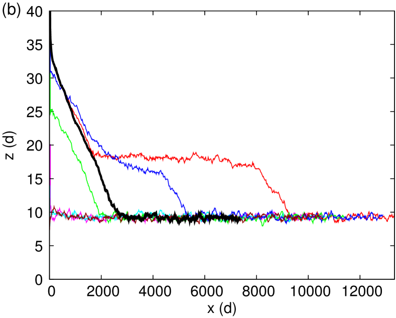
Figure 24: Tracer trajectories z-x (in color) measured in small bead diameters ($d$) in a 3D flow ($h_{max}=0.223$ m (37$d$)) with: (a) 10%, (b) 5% of tracers ($d_{t}/d=8$). Trajectory (thick black) of an identical single tracer released at the surface.

Figure 24 compares the trajectories of a single tracer and of several tracers (5% and 10%) in the case of a thick flow ($h_{max}=0.223$ m $\simeq 37d$). Tracers are initially randomly placed. The tracer trajectories reveal a succession of displacements: horizontal displacements (the tracers cannot move downwards due to the steric exclusion effect) alternated with downward displacements (with a slope less steep than the case of a single tracer). In the case of multiple tracers, the overall downward displacement is slower than that of a single tracer. The depth equilibrium position of the lowest layer in the case of multiple tracers is rapidly identical to the depth of one single tracer. For a 10% volume fraction, three, then two, layers of tracers form in the lower part the flow (Fig. 24(a)). Successive down cascading from one layer to another corresponds to an increase in the local fraction of the lowest layers. Very rare up-motions of tracers are observed. For 5% volume fraction (Fig. 24(b)), the downward slopes of a single tracer trajectory and of multiple tracer trajectories can even be comparable. Only one layer of tracers is present at the end, whose depth is identical to that of a single tracer.

First, the tracer fraction has no influence on the depth of the lowest layer. Consequently, it is possible to compare experimental and numerical data using the lowest numerical trajectories, and the lowest experimental tracer depths. The main effect of the increased fraction (5 or 10%) is the persistence of a second, possibly a third layer above the basal layer of tracers which is full and cannot include any more tracers. For this reverse segregation, there is an asymmetric upwards spread of the tracer positions, with a position distribution maximum at the lowest layer depth.

Secondly, the convergence to the final state of segregation is longer to establish for 5 or 10% of tracers than for one single tracer. Even though some individual downward velocities are locally the same, it takes time for tracers to move from one layer to another. Even though the global segregation pattern is rapidly obtained (around $2000-4000d$), the distance of convergence is so long (around $10000d$) that it is not reachable in usual laboratory conditions. These values are to be compared with experiments in channel with thicknesses from $28d$ to $45d$, and a surface pattern obtained at 70 cm WiederseinerAncey11 . Nevertheless, in our simulations, the depth of the lowest trajectory is rapidly defined for thick flows (Fig. 24). In our previous experiments, flows and deposits sometimes presented a thickness larger than 37$d$. To see how such a thickness could affect the previous results, one simulation is performed with $h_{max}=100d$, 10% of tracers and $d_{t}/d=8$ corresponding to an equilibrium reverse depth (Fig. 25). The number of basal layers increases, because for a constant volume fraction the number of tracers increases with the flow thickness. As several layers of tracers develop (instead of 2 or 3) and as tracers cascade between layers, the time and the distance needed for convergence strongly increase (Fig. 25). For experiments done with $d=300-400$ $\mu$m particles, a distance of convergence of $100000d$ requires a plane of 35 m. Nevertheless, the results for $h_{max}=100d$ are similar to those for $37d$ (Fig. 24): reverse segregation is obtained, the bottom layer depth at $9d$ (equal to the single tracer depth), and the formation of several layers of tracers. For larger size ratios, we may expect shorter convergence times and distances, since a single larger tracer reaches its equilibrium depth faster (Figs. 16(b) and 17, or 23).

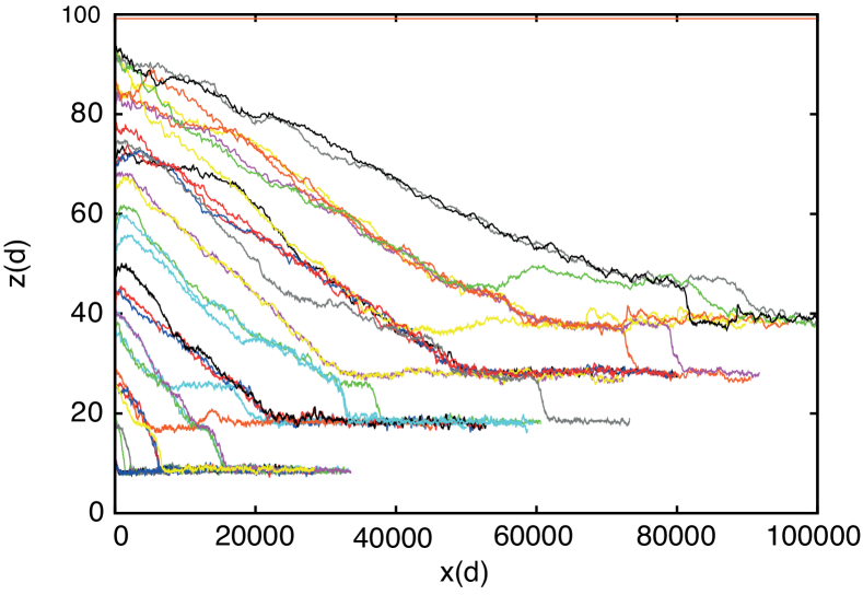
Figure 25: Trajectories (z-x) of a few tracers (10%, $d_{t}/d=8$) in a 3D very thick flow ($h_{max}=$100$d$) measured in small bead diameters ($d$).

Measurement of the segregated positions is made for 5% of tracers, in a thick flow $h_{max}=0.223$ m and for several size ratios in an interval around the value 4.3, i.e., the reversal transition of a single tracer position from surface to bottom (Fig. 26). The segregated position of several tracers at a given moment also presents a reversal, evolving from the surface to intermediate depths, and then to reverse depths. The standard deviation is small enough to consider that segregation occurs: tracers are not spread all through the bed, but regrouped near the mean position, especially for surface and reverse segregations. We then quantitatively compare the results for a single tracer ($h$ is the mean on the trajectory) and for several segregated tracers, and further down with experimental results on several tracers. Except minor differences, the two curves are very close. For small size ratios ($\leqslant 4$), mean depths are the same, but there is an increase in standard deviation for several tracers. The deviation includes both the trajectory fluctuations and the interaction between tracers. For size ratios $4.2\leqslant$ $d_{t}/d$ $\leqslant 4.7$, larger standard deviations and an upshift of mean depths are observed for several tracers, giving a smoother transition. For larger size ratios ($\geqslant 5$), the upshift disappears, and only larger standard deviations are observed for several tracers (note that for ratios above 8, all beads fit in the lowest layer, giving the same standard deviations as a single tracer). As the mean depth of a single tracer and those of several tracers are almost identical, it confirms the hypothesis that the segregation process for this low fraction is a regrouping of near non-interacting tracers at the same equilibrium depth, because this depth depends only on the size ratio. Studying a single tracer is valuable for understanding the segregation phenomena for a low fraction of tracers. With this low fraction, we observe successively surface segregation, intermediate segregation, and reverse segregation when increasing the size ratio. The reversal from surface to bottom happens for a size ratio (around 4.5) similar to the reversal size ratio for a single tracer(around 4.3). One consequence of the smoother transition than for a single tracer is the disappearance of the empty central region where no single tracer stabilizes in a thick flow (Fig. 20). For these fractions, there is a thick central layer of intermediate segregation. In the case of multiple tracers, the segregation pattern organizes in three layers (surface, intermediate and reverse), very much like the equilibrium depths of a single tracer in a thin flow.

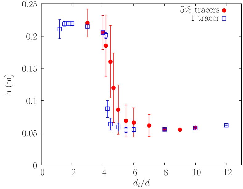
Figure 26: Equilibrium depths versus size ratio in a 3D flow ($h_{max}=0.223$ m) for: a single tracer (blue $\square$), 5% of tracers (red $\bullet$). Error bars show the standard deviation, but are only partly representative of the vertical spread of individual tracer positions which can be asymmetric, never higher than the surface or lower than the reverse position (see Fig. 24).

IV.2.7 Comparison with experiments in channel

Experiments were performed by the sudden release of 1 kg of an initially homogeneous mixture of glass beads with 10% of large tracers, in a 6 cm wide, 1 m long rough channel inclined with a slope about 26.5^∘ (more details in Thomas00 ). Flows were observed to be 1 to 2 cm thick, with deposits aggraded over 2 to 5 cm thick after the flow had been stopped by a perpendicular wall, or by the change of slope to horizontal. On cross-sections of the deposit, the segregation pattern could be separated in three main cases, depending on the size ratio: (1) the small size ratios (1.75, 2, 2.14, 3.5) (resp. for tracer diameter 0.35, 0.7 or 3, 1.5, 0.7 mm) for which all tracers were at the surface with a small standard deviation, (2) the 4.3 ratio (for 3 mm tracers) for which tracers were rather everywhere (surface and inside), and (3) the large ratios (5.9, 8.6, 10.4, 10.7, 15, 21.4, 44) (resp. for tracer diameter 3, 3, 0.7, 7.5, 3, 7.5, 3 mm) for which tracers were found inside, with a small layer free of tracers near the surface. Decrease in the mean position of tracers and in their standard deviation was observed when increasing the size ratio (for these $d_{t}/d\geqslant 4.3$).

The three patterns agree with the three types of tracer mean depth found in the simulations for several or for a single tracer (Fig. 26). The upper limit of the transition between surface and reverse segregations is experimentally found for 4.3. As this transition numerically occurs between 4.2 and 4.3 for one tracer and between 4.2 to 4.7 for 5% of tracers, the agreement is very good. But experimental standard deviations are large, not only for ratio 4.3, but for all larger size ratios, which is not observed in simulations at high size ratios. Nevertheless, standard deviations decrease with the size ratio in both experiments and simulations.

Three experiments were done with a wall to stop the flow at various distances from the start (30, 60 and 90 cm). Tracers were 3 mm, and small beads were 300-400 $\mu$m (size ratio 8.6). Tracers were found inside the deposit, with no major differences in the segregation pattern. But the mean depth of tracers in a cross-section taken at the same distance from the end wall (for example at 10 cm), showed a slight decrease passing from the 30 cm to the 60 cm, and to the 90 cm long experiment. The convergence to a final mean position was still developing at the time when the flow stopped. We conclude that all our experimental data, established for a 90 cm traveling distance, do not concern a perfect stationary state. This convergence distance is compatible with the simulations, where a stationary state is not reached at $2500d$ (equivalent to 90 cm) for flows of $37d$ (equivalent to 1.3 cm) (Fig. 24) or of $100d$ (equivalent to 3.5 cm) (Fig. 25). The fact that experimental standard deviations are larger than numerical ones can be explained by this non-fully converged state. It can also be explained by the use of 10% of tracers instead of 5%. The decreases in the experimental mean depth and standard deviation with increasing size ratios are compatible with a better convergence towards the reverse position. This better convergence is compatible with the faster migration of one single tracer when increasing the size ratio (comparing Figs. 16(b) and 17, or Fig. 23). This also explains why reverse segregation is experimentally nearly reached for the ratio 44, despite a quite short channel.

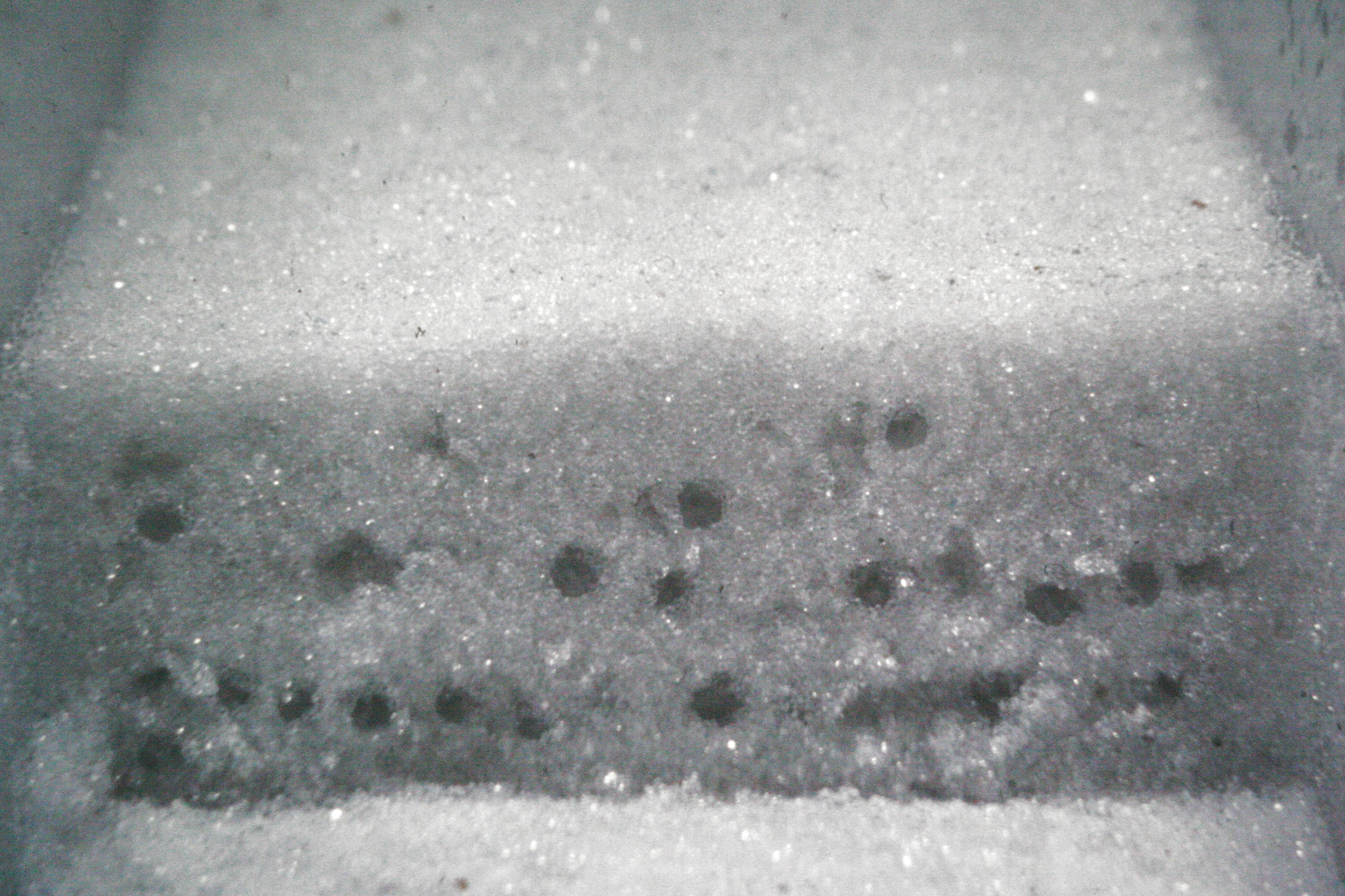
Figure 27: Cross-section of the deposit in a 1 m long and 6 cm wide chute flow experiment. The flow is composed of glass beads: 90% of 300-400 $\mu$m and 10% of 3 mm.

In the simulations (Figs. 24(a) and 25), for traveling lengths corresponding to experiments (90 cm=2500$d$), tracers above the first layer do not organize in superimposed layers like those obtained at the end of the simulations. For such a short flowing distance, the first bottom layer is well defined and the second layer is in formation. The other layers are still emerging and have not reached their final depth yet. Indeed, in experiments, most sections presented tracers organized in one bottom layer (Fig. 27), and sometimes in a blurred second layer. Experimental measurements of this bottom layer depth were done at a distance between 15 and 30 cm from the end wall. We tried to avoid perturbations due to the collision with the end wall and the possible local variations of the tracer fraction near the flow front. For size ratios from 4.3 to 8.6, the bottom layer depth was experimentally measured between $10$ and $11.5d$ with randomness (and $13d$ for size ratio 15, above our simulation range). These values are close to the $9$ to $10.2d$ values numerically found for size ratios from 5 to 12 (Fig. 18).

Even though the stationary stage has not been reached in our experiments, experimental data reproduce well the existence of the bottom layer and its depth, the reversal between surface and reverse segregations, the variation of the associated standard deviations, and the exact size ratio ($d_{t}/d=4.3$) for which the reversal occurs. Moreover, the numerical study has shown that experimental tracers settled inside ($d\geqslant 5.9$) correspond to non-converged states of reverse segregation at different degrees of convergence.

Simulation and experiment results both show that the size ratio 4.3 induces intermediate segregation of the tracers, for which the spread of the experimental positions is maximum (in addition, it is experimentally obtained for a non-fully converged system). The result is a nearly homogeneous mixture. This experimental spread of tracers all through the deposit is compatible with the numerical results obtained for a converged state: a quite large standard deviation combined with a mean position at mid-height. But longer times of convergence, and effects coming from the increase in the tracer fraction up to 10% might also be involved in the experimental process for explaining the tracer spread. For that reason, the range of size ratios around 4.3 needs further investigations. Nevertheless, combining an intermediate segregation and an appropriate tracer fraction could be a means to prevent any segregation during a flow.

V Conclusion

In 3D granular flows, the selection of an equilibrium depth of a large tracer depends mainly on the size ratio between the tracer and the small beads, and to a lesser extent on the nature of the flow. Comparison between depths of single tracers and mean depths of several tracers (3 to 10%) shows that the stabilization of one tracer and the segregation process select identical equilibrium depths. In that case, the segregation is the regrouping of non-interacting large tracers at the same equilibrium depth.

In a tumbler, a precise study of trajectories has shown that the depth is established during the flowing phase and is recorded in the static rotating part. The flow substratum is a loose granular material whose boundary with the flowing layer is difficult to define, but trajectories of the largest size ratios seem to place tracers at the bottom of the flow. Thus surface positions, intermediate positions with deeper and deeper depths toward reverse positions are observed when increasing the size ratio between the tracer and the small particles. The transition between surface and reverse depths is progressive, and a large range of tracer size ratios is found to be at intermediate depths.

For all 3D flows down a rough incline, the reversal also happens when increasing the size ratio. Two cases are clear: positions near the surface, which corresponds to tracers at the surface, or to non visible tracers, just under the surface (surface and intermediate depths), and positions of tracers floating at or very close to the bottom (intermediate and reverse depths). The existence of intermediate positions near half-height depends on the flow thickness. For thick flows, the reversal between surface and bottom positions is sharp, with no tracers stabilized around mid-height. For thin flows, the reversal is progressive and tracers stabilize at every intermediate depth inside the flow. We conclude that, in 3D, the tracer position is also determined by the type of substratum (solid or loose) and the flow thickness.

For multiple tracer flows on 3D incline (5 to 10%), the three segregation patterns (surface, intermediate, reverse) are observed when increasing the size ratio, corresponding to the three types of depth stabilization of a single tracer. The transition is smoother and happens at the same size ratio (around 4.3) for simulations and experiments, corresponding to single tracer reversal. But reverse segregation is long to establish, and a large spread in the positions remains over a long traveling distance. During this travel, the flows (with size ratio above 5) can be considered as nearly homogeneous, except near their surface where only small particles are present. The intermediate case (size ratio 4.3) remains almost homogeneous. The choice of reverse and especially intermediate positions could be an opportunity to maintain a homogeneous mixture for usual industrial transfers. Further studies are needed to set the precise parameter range where these processes can be used.

The case of 2D flows has been studied in tumblers and inclines. For small size ratios, the position of tracers relative to the free surface behaves similarly in 2D and 3D, although deeper positions are found for large size ratios in 3D. The dependency of the stabilized depth on the size ratio is similar but weaker in 2D both in tumbler and on incline. Moreover for the largest size ratio tracers on 2D inclines, the reverse positions do not exist. Tracers stabilize at intermediate positions near mid-height and their position scales with the flow thickness contrarily to the 3D case. In 2D tumblers, the equilibrium position evolution with size ratio is also weaker, with a shifted maximum, and leads to an intermediate radial position of equilibrium for the largest tracers. However, the position of these largest tracers does correspond to a reverse depth comparable to that of the 3D case, but this depth is obtained for larger size ratios than in 3D. The difference between 2D and 3D, probably due to a granular packing compacity difference, does not emerge in all processes in the same manner. The highest care should be taken before extrapolating results of studies between 2D and 3D cases.

- (1) J. C. Williams, Powder Technol. 15, 245 (1976).
- (2) J. Duran, J. Rajchenbach, and E. Clément, Phys. Rev. Lett. 70, 2431 (1993).
- (3) H. M. Jaeger, S. R. Nagel, and R. P. Behringer, Rev. Mod. Phys. 68, 1259 (1996).
- (4) F. Cantelaube and D. Bideau, Europhys. Lett. 30 (3), 133 (1995).
- (5) K. Hutter, B. Svendsen, and D. Rickenmann, Contin. Mech. Thermodyn. 8 (1), 1 (1996).
- (6) J. M. Ottino and D. V. Khakhar, Annu. Rev. Fluid Mech. 32 (1), 55 (2000).
- (7) J. M. N. T. Gray, M. Shearer, and A. R. Thornton, Proc. R. Soc. A 462, 947 (2006).
- (8) C. P. Schlick, Y. Fan, P. B. Umbanhowar, J. M. Ottino, and R. M. Lueptow, J. Fluid Mech. 765, 632 (2015).
- (9) M. Larcher and J.T. Jenkins, Phys. Fluids 25, 113301 (2013).
- (10) M. Larcher and J.T. Jenkins, J. Fluid Mech. 782, 405 (2015).
- (11) D.V. Khakhar, J.J. McCarthy, and J.M. Ottino, Chaos 9 (3), 594 (1999).
- (12) S.B. Savage and C.K.K. Lun, J. Fluid Mech. 189, 311 (1988).
- (13) J. M. N. T. Gray, M. Shearer, and A. R. Thornton, Proc. R. Soc. A 461, 1447 (2005).
- (14) L.B.H. May, L.A. Golick, K.C. Phillips, M. Shearer, and K.E. Daniels, Phys. Rev. E 81, 051301 (2010).
- (15) D. R. Tunuguntla, O. Bokhove, and A. R. Thornton, J. Fluid Mech. 749, 99 (2014).
- (16) Y. Fan, C.P. Schlick, P.B. Umbanhowar, J.M. Ottino, and R.M. Lueptow, J. Fluid Mech. 741, 252 (2014).
- (17) C.P. Schlick, A.B. Isner, B.J. Freireich, Y Fan, P.B. Umbanhowar, J.M. Ottino, and R.M. Lueptow, J. Fluid Mech. 797, 311 (2016).
- (18) Y. Fan and K. M. Hill, Phys. Rev. Lett. 106, 218301 (2011).
- (19) Y. Fan and K. M. Hill, Phys. Rev. E 92, 022211 (2015).
- (20) B. Marks, P. Rognon, and I. Einav, J. Fluid Mech. 690, 499 (2012).
- (21) L. Staron and J.C. Phillips, Comp. Part. Mech. 3 (3), 367 (2016).
- (22) S. Wiederseiner, N. Andreini, G. Épely-Chauvin, G. Moser, M. Monnereau, J. M. N. T. Gray, and C. Ancey, Phys. Fluids 23, 013301 (2011).
- (23) D.R. Tunuguntla, T. Weinhart, and A.R. Thornton, Comp. Part. Mech. DOI: 10.1007/s40571-016-0136-1 (2016).
- (24) D.R. Tunuguntla, T. Weinhart, and A.R. Thornton, Comp. Part. Mech. 3 (3), 349 (2016).
- (25) L.A. Golick and K.E. Daniels, Phys. Rev. E 80 (4), 042301 (2009).
- (26) Y. Ding, N. Gravish, and D.I. Goldman, Phys. Rev. Lett. 106, 028001 (2011).
- (27) F.Q. Potiguar and Y. Ding, Phys. Rev. E 88, 012204 (2013).
- (28) F. Guillard, Y. Forterre, and O. Pouliquen, Phys. Fluids 26, 043301 (2014).
- (29) F. Guillard, Y. Forterre, and O. Pouliquen, J. Fluid Mech. 807, R1, (2016).
- (30) N. Thomas, Phys. Rev. E 62, 961 (2000).
- (31) T. Shinbrot and F. J. Muzzio, Phys. Rev. Lett. 81 (20), 4365 (1998).
- (32) A. P. J. Breu, H.-M. Ensner, C. A. Kruelle, and I. Rehberg, Phys. Rev. Lett. 90 (1), 014302 (2003).
- (33) J. Ellenberger, C. O. Vandu, and R. Krishna, Powder Technol. 164 (3), 168 (2006).
- (34) D. Hong, P. V. Quinn, and S. Luding, Phys. Rev. Lett. 86, 3423 (2001).
- (35) J. B. Knight, H. M. Jeager, and S. R. Nagel, Phys. Rev. Lett. 70, 3728 (1993).
- (36) G. Félix and N. Thomas, Phys. Rev. E 70, 051307 (2004).
- (37) A.R. Thornton,T. Weinhart, S. Luding, and O. Bokhove, Int. J. Mod. Phys. C 23 (08), 1240014 (2012).
- (38) M. Rahman, K. Shinohara, H.P. Zhu, A.B.Yu, and P. Zulli, Chem. Eng. Sci. 66, 6089 (2011).
- (39) J. Schäfer, S. Dippel, and D. E. Wolf, J. Phys. 1 (France) 6, 5 (1996).
- (40) P. A. Cundall and O. D. L. Starck, Géotechnique 29, 47 (1979).
- (41) T. G. Drake and R. L. Shreve, J. Rheol. 30, 981 (1986).
- (42) S. F. Foerster, M. Y. Louge, H. Chang, and K. Allia, Phys. Fluids 6, 1108 (1994).
- (43) Z. Zaman, U. D’Ortona, P. B. Umbanhowar, J. M. Ottino, and R. M. Lueptow, Phys. Rev. E 88, 012208 (2013).
- (44) N. Taberlet, M. Newey, P. Richard, and W. Losert, J. Stat. Mech. P07013 (2006).
- (45) P. Chen, J. M. Ottino, and R. M. Lueptow, New J. Phys. 13, 055021 (2011).
- (46) G. H. Ristow, Pattern Formation in Granular Materials (Springer-Verlag, Berlin, 2000).
- (47) C. S. Campbell, J. Fluid Mech. 465, 261 (2002).
- (48) L. E. Silbert, G. S. Grest, R. Brewster, and A. J. Levine, Phys. Rev. Lett. 99, 068002 (2007).
- (49) K. M. Hill and D. S. Tan, J. Fluid Mech. 756, 54 (2014).
- (50) G. Félix, V. Falk, and U. D’Ortona, Eur. Phys. J. E 22, 25 (2007).
- (51) G. Félix and N. Thomas, Earth Planet. Sci. Lett. 221, 197 (2004).
- (52) N. Thomas and U. D’Ortona, in prep.