Entropic Lattice Boltzmann Model for Charged Leaky Dielectric Multiphase Fluids in Electrified Jets

Abstract

We present a lattice Boltzmann model for charged leaky dielectric multiphase fluids in the context of electrified jet simulations, which are of interest for a number of production technologies including electrospinning. The role of non-linear rheology on the dynamics of electrified jets is considered by exploiting the Carreau model for pseudoplastic fluids. We report exploratory simulations of charged droplets at rest and under a constant electric field, and we provide results for charged jet formation under electrospinning conditions.

I Introduction

The dynamics of charged leaky dielectric jets present a major interest, both as an outstanding problem in non-equilibrium thermodynamics, as well as for its numerous applications in science and engineering Yarin et al. (2014); Wendorff et al. (2012); Pisignano (2013). In particular, the recent years have witnessed a surge of interest towards the manufacturing of electrospun polymeric nanofibers, mostly on account of their prospective applications, such as tissue engineering, air and water filtration, optoelectronics, drug delivery and regenerative medicine Pisignano (2013); Frenot and Chronakis (2003); Huang et al. (2003). As a consequence, several experimental studies have focused on the characterization and production of one-dimensional elongated nanostructures Li et al. (2004); Greiner and Wendorff (2007); Carroll et al. (2008); Huang et al. (2003); Persano et al. (2013). Electrospun nanofibers are typically produced at laboratory scale via the uniaxial stretching of a leaky dielectric jet, which is ejected at a nozzle from an electrified charged polymer solution. The charged jet elongates under the effect of an external electrostatic field applied between the spinneret and a conductive collector and eventually undergoes electromechanical (e.g., whipping) instabilities due to various sources of disturbance, such as mechanical vibrations at the spinneret, hydrodynamic friction with the surrounding fluid and others Reneker et al. (2000). While such instabilities can be detrimental in some respect, making an accurate position of individual fibres on target substrates very hard, in other experiments they are sought for since they result in thinner cross sections, hence finer electrospun fibres, as they hit the collector Frenot and Chronakis (2003). This follows from a plain argument of mass conservation: whipping instabilities generate longer jets, hence thinner cross sections Feng (2003).

The computational modelling of the electrospinning process is based on two main families of techniques: particle methods and Lagrangian fluid methods. The former is based on the representation of the polymer jet as a discrete collection of discrete particles (beads) connected via elastic springs with frictional coupling (dissipative dashpots) and interacting via long-range Coulomb electrostatics Reneker et al. (2000); Lauricella et al. (2015a, 2016a, 2016b). The latter, on the other hand, describes the jet as a continuum media, obeying the Navier-Stokes equations for a charged fluid in Lagrangian form Ganan-Calvo (1997); Hohman et al. (2001a); Yarin et al. (2001a). Both methods are grid-free, hence well suited to describe abrupt changes of the jet morphology without taxing the grid resolution, as it is the case for Eulerian grid methods.

In this respect, grid-based methods, such as Lattice Boltzmann methods (LBM), are not expected to offer a competitive alternative to the two aforementioned class of methods. Nevertheless, owing to its efficiency, especially on parallel computers, and its flexibility towards the inclusion of physical effects beyond single-phase hydrodynamics, it appears worth exploring the possibility of using LBM also in the framework of electrified fluids and jets. For instance, in the last decade significant improvements in LBM for modelling microfluidic flows containing electrostatic interactions have been achieved Li and Kwok (2003); Kupershtokh and Medvedev (2006), opening new applications of LBM in electrohydrodynamic problems Huang et al. (2007); Gong et al. (2010); Medvedev (2010); Bararnia and Ganji (2013); Kupershtokh (2014). In particular, LBM was successfully employed to simulate deformations and breakup of conductive vapour bubbles, bubble deformation due to electrostriction, dynamics of drops with different electric permittivity. All these investigations usually exploit the approach originally introduced by A. L. Kupershtokh and D. A. Medvedev Kupershtokh and Medvedev (2006), where dielectric liquids are assumed with zero free charge density, so that the charge carriers are essentially locally bounded to the material Landau et al. (2013). Within this assumption, charge carriers are explicitly modelled by a convective transport equation solved by a second LB solver, taking into account the rates of ionization and recombination of charge carriers fluctuating around a local value (distribution) of equilibrium.

In the 1960s, G. I. Taylor provided several considerations for dealing with electrified fluid in a series of papers Taylor (1964, 1966, 1969). In particular, Taylor discovered that a moving charged fluids cannot be considered either as a perfect dielectric or as a perfect conductor. Instead, the fluid acts as a "leaky dielectric liquid", where a non-zero free charge is mainly accumulated on the interface between the charged liquid and the gaseous phase Saville (1997). As a consequence, the charge produces electric stresses different from those observed in perfect conductors or perfect dielectrics. Indeed, in the last cases, the charge induces a stress which is perpendicular to the interface, altering the interface shape to balance the extra stress. In the electrospinning process, the non-zero electrostatic field tangent to the liquid interface produces a non-zero tangential stress on the interface which is balanced from the viscous force Hohman et al. (2001a).

The present work exploits the entropic variant of LBM Karlin et al. (1999). In particular, the use of the entropic lattice Boltzmann method (ELBM) allows to extend the LBM application also in presence of intense electrostatic forces, acting on charged leaky dielectric liquids, which is of main interest for modelling the electrospinning process. In this context, the largest part of the charge is modelled to lie along the interface between the liquid and the gaseous phase in similarity with previous works Hua et al. (2008); Li et al. (2011). Further, the present ELBM is generalized to the case of non-Newtonian flows with a shear-thinning viscosity in order to account the rheological properties of electrospun jets. Here, we adopt the entropic approach introduced by S. Ansumali and I. V. Karlin in Ref Ansumali and Karlin (2002) in order to preserve locally the second principle (H- theorem) also in presence of sharp changes in the fluid viscosity and structure.

The paper is organised as follows. In section II we present the basic features of the LB extension to the case of charged multiphase fluids. In sections III, we present results for the case of charged multiphase fluids at rest and we report on preliminary results for charged multiphase jets under conditions related to electrospinning experiments.

II Model

We consider a single species, charged fluid as composed of point-like particles and neglect correlations stemming from excluded volume interactions. Following Boltzmann’s description, the state of the fluid is determined by the distribution function $f_{p}(\vec{r},t)$ being the probability of finding at time $t$ the fluid at position $\vec{r}$ and moving with discrete velocity $\vec{c}_{p}$, with $p=1,b$ given $b$ the number of lattice directions. Here, the velocities $\vec{c}_{p}$ are also viewed as vectors connecting a lattice site $\vec{r}$ to its lattice neighbours. The ELBM equation reads

$$f_{p}(\vec{r}+\vec{c}_{p}\Delta t,t+\delta t)=f_{p}(\vec{r},t)-\alpha\beta(f_{p}-f^{eq}_{p}(\rho,\vec{u}))+S_{p}(\vec{r},t),$$ (1)

where the product $\alpha\beta$ plays the role of a collision frequency, $S_{p}$ is a source term (see below), and $f^{eq}_{p}$ is the Maxwell-Boltzmann distribution computed at density $\rho$ and velocity $\vec{u}$ Chikatamarla et al. (2006). The macroscopic variables are given by the density $\rho=\sum_{p}f_{p}$ and the fluid velocity $\vec{u}=1/\rho\sum_{p}\vec{c}_{p}f$. In the following, we refer to lattice units where the mesh spacing and timestep $\Delta t$ are conveniently set to unity. Also, we adopt the so-called D2Q9 scheme, composed by 8 discrete speeds (connecting first and second lattice neighbors) and one extra null vectors accounting for particles at rest. In this scheme, Here, the $f^{eq}_{p}$ are chosen as a second-order Mach-number expansion

$$f_{p}^{eq}=w_{p}\rho\left[1+\frac{\vec{u}\cdot\vec{c}_{p}}{c^{2}_{s}}+\frac{(\vec{u}\cdot\vec{c}_{p})^{2}-c^{2}_{s}u^{2}}{2c^{4}_{s}}\right]$$ (2)

where the $w_{p}$ are weights equal to 4/9 for the rest particles, 1/9 and 1/36 respectively for the smallest and largest velocities $\vec{c}_{p}$, and $c_{s}$ is the speed of sound that in lattice units is equal to $1/\sqrt{3}$. At the same time, we consider a unit fluid molecular mass, so that the thermal energy is equal to $k_{B}T=c^{2}_{s}$ with $k_{B}$ the Boltzmann constant and $T$ the temperature. Following the approach of Refs. Dorschner et al. (2016); Chikatamarla et al. (2006); Ansumali and Karlin (2002), the factor $\beta$ in Eq. 1 depends on the kinematic viscosity $\nu$ by the relation

$$\beta=\frac{c^{2}_{s}}{2\nu+c^{2}_{s}},$$ (3)

while $\alpha$ is the largest value of the over-relaxation parameter so that the local entropy reduction can be avoided, ensuring the H- theorem. In particular, $\alpha$ is computed as the root of the scalar nonlinear equation Ansumali and Karlin (2002); Karlin et al. (1999)

$$H\left(f+\alpha(f^{eq}-f)\right)=H\left(f\right),$$ (4)

where $H$ denotes the Boltzmann’s entropy function, defined in discrete form Ansumali et al. (2003) as

$$H\left(f\right)\equiv\sum_{p}f_{p}\ln\left(\frac{f_{p}}{w_{p}}\right).$$ (5)

In Eq. 1, the source term $S_{p}$ takes into account the global effect of all the internal and external forces $\vec{F}$. This is assessed by the exact difference method proposed by Kupershtokh et al. Kupershtokh et al. (2009), which reads

$$S_{p}=f_{p}^{eq}\left(\rho,\vec{u}+\Delta\vec{u}\right)-f_{p}^{eq}\left(\rho,\vec{u}\right),$$ (6)

where $\Delta\vec{u}=\vec{F}/\rho$. In bulk conditions, the ELBM is intrinsically second-order accurate in space and time, and, in order to ensure the same accuracy in presence of forces, the local velocity is taken at half time step

$$\rho\vec{u}=\sum_{p}f_{p}(\vec{r},t)\vec{c}_{p}+\frac{1}{2}\vec{F}.$$ (7)

Here, the total body force $\vec{F}=\vec{F}_{int}+\vec{F}_{el}$ includes the inter-particle force $\vec{F}_{int}$ and the electric force $\vec{F}_{el}$. The electric force acting on the boundary point $\vec{r}$ between a gas and a fluid with the local non-uniform permittivity $\varepsilon(\vec{r})$ in an electric field $\vec{E}$ reads Landau et al. (2013); Saville (1997)

$$\vec{F}_{el} =q\vec{E}-\frac{1}{2}|E|^{2}\nabla\varepsilon+\frac{1}{2}\nabla\left(|E|^{2}\rho\frac{\partial\varepsilon}{\partial\rho}\right)$$ (8)

$$=q\vec{E}+\frac{1}{2}\rho\frac{\partial\varepsilon}{\partial\rho}\nabla|E|^{2},$$

where $q$ is the local free charge carried on the fluid. In the last Eq., the vacuum permittivity $\varepsilon_{0}$ was assumed equal to 1 as in the Gaussian centimetre-gram-second (cgs) unit system, so that the charge in lattice units is $length^{3/2}\,mass^{1/2}\,time^{-1}$ in similarity with the statcoulomb definition (note that Coulomb’s constant is also 1). For the sake of convenience, we report in Appendix A the units conversion Table 1 in cgs dimensions from lattice units for several physical quantities shown in the following. As in Ref. Kupershtokh and Medvedev (2006), we consider a fluid with permittivity $\varepsilon=1+\rho/\rho_{0}$ with $\rho_{0}$ an arbitrary constant (in the following taken for simplicity equal to 1) so that it is $\rho(\partial\varepsilon/\partial\rho)=\varepsilon-1$. As a consequence, Eq. 8 reduces to

$$\vec{F}_{el}=q\vec{E}+\frac{\varepsilon-1}{2}\nabla|E|^{2}.$$ (9)

In the following, we assume that the magnetic induction effects can be neglected so $\nabla\times\vec{E}=0$, and the system follows the Gauss law $\nabla\cdot(\varepsilon\vec{E})=q$. Since $\vec{E}=-\nabla\phi$ with $\phi$ the electric potential, the Poisson equation $div(\varepsilon(\vec{r})\nabla\phi)=-q(\vec{r})$ can be solved at each lattice node $\vec{r}$, given the boundary conditions of the system and the local charge $q(\vec{r})$ at the node (specified below). In particular, we determine the electric potential by solving numerically the two-dimensional Poisson equation by means of a SOR (Successive Over-Relaxation) algorithm and the Gauss-Seidel method Quarteroni and Valli (2008). Note that the Poisson equation includes the non-uniformity of the permittivity $\varepsilon(\vec{r})$, and it is solved on-the-fly during the simulation. Hence, the electric force $\vec{F}_{el}=-q\nabla\phi$ is added into the ELBM by Eq. 6.

Since we are modelling a leaky dielectric fluid, we assume that the free charge in the system is mainly distributed over the liquid-gaseous interface. Further, in similarity to previous electrospinning models Hohman et al. (2001a); Yarin et al. (2001a), the relaxation time of free charge in the system is assumed to be irrelevant. In other words, the free charge in bulk liquid relaxes to the liquid interface in a smaller time than any other characteristic time in the system Gañán-Calvo (2004). This is a well-established assumption of a leaky dielectric fluid (for further details see Ref. Saville (1997)). The liquid charge in the point $\vec{r}$ is given as

$$q=q_{b}+q_{s},$$ (10)

which is the sum of a surface charge $q_{s}$ and a small bulk term $q_{b}$. The bulk term $q_{b}$ is taken as

$$q_{b}(\vec{r})=Q_{b}\frac{\rho(\vec{r})\,\theta(\rho(\vec{r});\rho_{0})}{\int\rho(\vec{r})\,\theta(\rho(\vec{r});\rho_{0})d\vec{r}},$$ (11)

where $Q_{b}$ denotes the total charge in the bulk, the denominator acts to keep constant the charge due to the charge conservation principle, and $\theta(\rho;\rho_{0})$ denotes a smoothed version of the Heaviside step function switching from zero to one at $\rho_{0}$ (equal to 1 in all the following simulations) in order to select only the liquid phase. The term $q_{s}$ is modeled as a proportional to the absolute density gradient

$$q_{s}(\vec{r})=Q_{s}\frac{|\nabla\rho(\vec{r})|^{2}}{\int|\nabla\rho(\vec{r})|^{2}d\vec{r}},$$ (12)

where $Q_{s}$ denotes the total charge over the surface, and the denominator ensures the charge conservation principle as in the previous case. This approach is usually referred to as the constant surface charge model. It is important to highlight that such charge model is different from the method adopted by Kupershtokh et al. Kupershtokh and Medvedev (2006), where the charge carriers are treated by using an additional LB component with zero mass (passive scalar) to model the polarizability of a dielectric liquid with zero free charge. Since in the present model the charge is directly modelled over the interface, we do not need to introduce any extra LB component to model the surface charge. Indeed, the constant surface charge model was already adopted in Refs Hua et al. (2008); Li et al. (2011) as a strategy to simplify the charge transport and distribution on the droplet interface. Nonetheless, the constant surface charge model fails in describing a distributed charge on the drop interface whenever the charge density is high, since the curvature surface alters the local charge density Hohman et al. (2001a). In order to address the issue, we assume that the curvature biases the surface charge density as in a conductive liquid, following the power-law introduced by I. W. McAllister McAllister (1990), which states

$$q_{s}=q_{s,max}(K/K_{max})^{\frac{1}{4}}.$$ (13)

Here, $K$ denotes the mean curvature $K=\nabla\cdot\widehat{n}$ with the local interface normal $\widehat{n}=\nabla\rho(\vec{r})/|\nabla\rho(\vec{r})|$ Spencer et al. (2010), while $q_{s,max}$ is the maximum surface charge at the maximum curvature $K_{max}$ chosen as a reference value for the system under investigation. It is worth to emphasize that treating a leaky dielectric as a conductive liquid is a simplification already made by several authors (e.g., G. Taylor Taylor (1964), A. Yarin et al. Yarin et al. (2001b) , etc.). For the sake of simplicity, we take in the following the maximum curvature $K_{max}$ equal to $K_{d}$ value, defined as the curvature doubling the local surface charge density. Thus, we rewrite Eq. 10 as

$$q(\vec{r})=Q_{b}\frac{\rho(\vec{r})\,\theta(\rho(\vec{r});\rho_{0})}{\int\rho(\vec{r})\,\theta(\rho(\vec{r});\rho_{0})d\vec{r}}+\\ +Q_{s}\frac{|\nabla\rho(\vec{r})|^{2}[1+(K/K_{d})^{\frac{1}{4}}]}{\int|\nabla\rho(\vec{r})|^{2}[1+(K/K_{d})^{\frac{1}{4}}]d\vec{r}}.$$ (14)

The total charge of the system is conserved and equal to $Q=Q_{b}+Q_{s}$.

In addition, the fluid is subjected to an internal thermodynamic force $\vec{F}_{int}$ promoting a phase separation, in similarity with the approach originally introduced by Mazloomi et al. Chikatamarla et al. (2015) in the context of the ELBM. The phase separation force is accounted for by means of the Shan-Chen method Huang et al. (2015); Falcucci et al. (2010). We construct the local force as

$$\vec{F}_{int}(\vec{r},t)=-G\,\psi(\rho(\vec{r},t))\sum_{p\in fluid}w_{p}\psi(\rho(\vec{r}+\vec{c}_{p},t))\vec{c}_{p}-\\ -G_{w}\,\psi(\rho(\vec{r},t))\sum_{p\in wall}w_{p}\psi(\rho(\vec{r},t))\vec{c}_{p},$$ (15)

with the sum $\sum_{p\in fluid}$ running over lattice nodes where the fluid is allowed, that is, not belonging to the wall, and $\sum_{p\in wall}$ runs over nodes belonging to the wall. $G$ and $G_{w}$ are fluid-fluid and fluid-wall interaction strengths, respectively. In Eq 15, $\psi$ is an effective number density, which is taken for simplicity $\psi(\rho)=\rho_{0}[1-\exp(-\rho/\rho_{0})]$, being $\rho_{0}$ an arbitrary constant Shan and Chen (1993) (in the following assumed equal to 1).

II.1 Extension to Non-Newtonian flows

In the electrospinning process, the rheological behaviour of polymeric liquid with shear-rate-dependent viscosity is expected to play a significant role in jet dynamics. As a consequence, we now generalize the present model to the case of non-Newtonian flows, in similarity with the approach reported in Refs Pontrelli et al. (2009); Gabbanelli et al. (2005); Aharonov and Rothman (1993). The shear-rate $\dot{\gamma}$ is a functional of the density distribution function $f$. In particular, the strain tensor $\mathbf{\Gamma}_{\eta,\delta}$ reads Pontrelli et al. (2009); Ouared and Chopard (2005)

$$\mathbf{\Gamma}_{\eta,\delta}=-\frac{1}{2\rho\tau c^{2}_{s}}\mathbf{\Pi}_{\eta,\delta},$$ (16)

where

$$\mathbf{\Pi}_{\eta,\delta}=\sum_{p}\left(f_{p}-f_{p}^{eq}\right)\vec{c}_{p\eta}\vec{c}_{p\delta},$$ (17)

is the the stress tensor with $\eta$ and $\delta$ running over the spatial dimensions. Note that $\tau$ in Eq. 16 is defined as the inverse of the product $\alpha\beta$, where $\alpha$ was computed by Eq. 4, and $\beta$ depends by Eq. 3 on the kinematic viscosity $\nu$. We now rewrite Eq. 16 as

$$\dot{\gamma}=\frac{\Pi}{\rho\tau(\dot{\gamma})c^{2}_{s}},$$ (18)

where $\dot{\gamma}$ and $\Pi$ are computed as matrix 2-norm $\dot{\gamma}=2||\mathbf{\Gamma}||_{2}$ and $\Pi=||\mathbf{\Pi}||_{2}$ of the shear and stress tensor Pontrelli et al. (2009), respectively. Note that in the last Eq. we exploit a constitutive relation between the kinematic viscosity $\nu$ and the shear-rate $\dot{\gamma}$, so that $\tau=\tau(\dot{\gamma})$. As a consequence, $\dot{\gamma}$ is computed as the root of the scalar nonlinear Eq. 18.

We should now consider the general trend observed in electrospun polymeric filaments Agarwal et al. (2016). As main features, we highlight that a polymeric spinning solution at low shear rate behaves as a quasi-Newtonian fluid with zero shear kinematic viscosity $\nu_{0}$, since the initial condition can be recovered, while at a high shear rate a non-reversible disentanglement is present. In particular, it is possible to identify a relaxation time $\lambda$ at which the shear-thinning starts, which is equal to the inverse value of the shear rate at that instant. At the very high shear rate, a quasi-Newtonian behaviour is again observed as soon as the alignment of the polymer chains is extremely high (almost complete). The last region is characterized by a final viscosity value (infinite viscosity $\nu_{\infty}$), which is lower than $\nu_{0}$.

In the present investigation, we exploit the Carreau model Johnson (2016), which is able to describe all the mentioned rheological properties. The Carreau model states that

$$\nu(\dot{\gamma})=\nu_{\infty}+\left(\nu_{0}-\nu_{\infty}\right)\left[1+\left(\lambda\dot{\gamma}\right)^{2}\right]^{(n-1)/2},$$ (19)

where $n$ is the flow index ($n<1$ for a pseudoplastic fluid). Obtained $\dot{\gamma}$ by resolving Eq. 18 and $\nu(\dot{\gamma})$ by Eq. 19, and assuming a slow variation of $\nu(\dot{\gamma})$ over the time $\Delta t$, the local parameter $\beta$ is finally estimated by Eq. 3. Note that a validation of a similar implementation in a LB scheme of the Carreau model was given in Ref. Pontrelli et al. (2009).

II.2 Summary of the model

To solve the Eq. 1, we exploit the method of splitting the model procedure into physical process stages. Hence, the time step is given by the sequential implementation of the following key points:

1. Compute the Boltzmann’s entropy function, and determine $\alpha$ by solving Eq. 4.

2. Solve the nonlinear Eq. 18 to compute the local rate strain $\dot{\gamma}$, and determine the local viscosity $\nu$ as a function of the rheological Eq. 19. Hence, determine $\beta$ from Eq. 3.

3. Compute the local charge $q$ by Eq. 14, and solve the Poisson equation for assessing the electric force $\vec{F}_{el}=-q\nabla\phi$.

4. Compute the phase separation force $\vec{F}_{int}$ by Eq. 15.

5. Apply the Eq. 1.

III Numerical results

III.1 Charged drop

In order to assess the properties of our implementation for charged multiphase systems, we have initially run a set of simulations modelling a charged leaky dielectric fluid system obeying the Shan-Chen equation of state Shan and Chen (1993). In order to assess the static behaviour, we take a two-dimensional periodic mesh made of 320 x 320 nodes, and prepare the system by creating a circular drop of density $\rho=2.0$ and radius $R=40$ in lattice units, immersed in the second background phase at lower density $\rho_{b}=0.16$. Further, the strength of non-ideal interactions was set equal to $G=-5$, $G/G^{o}_{crit}=1.25$ where $G^{o}_{crit}=-4$ is the critical Shan-Chen coupling at the critical density $\rho_{crit}=\ln 2$ in the absence of electric fields. Since we aim to model a leaky dielectric fluid, the ratio $Q_{s}/Q_{b}$ is taken equal to 10, so that the largest part of the charge lies over the surface. The total charge $Q=Q_{s}+Q_{b}$ was set equal to $2.13$, and $q(\vec{r})$ computed by Eq. 14. Whenever the Poisson equation is solved, a uniform negative charge is added to obtain a system with net charge zero. Hence, the electric force $\vec{F}_{el}=q(-\nabla{\phi})$ is added into the ELBM by Eq. 6, where $q$ is computed by Eq. 14 with $K_{d}$ equal to 1. The liquid is Newtonian with kinematic viscosity $\nu=1/6$.

The stationary configuration of the described system is obtained after 1000 time steps. Hence, we inspect the electric field (see Fig. 1) at rest conditions in order to analyze the balance of forces acting at the interface, including Shan-Chen pressure and capillary and electrostatic forces, the latter pointing normal to the interface (see panel b of Fig. 1). Here, we observe that the largest part of the electric field is located over the liquid surface where the charge distribution is higher. In particular, at the boundary of the drop the magnitude of the electric field $|\vec{E}|$ is equal to $3.5\cdot 10^{-3}$.

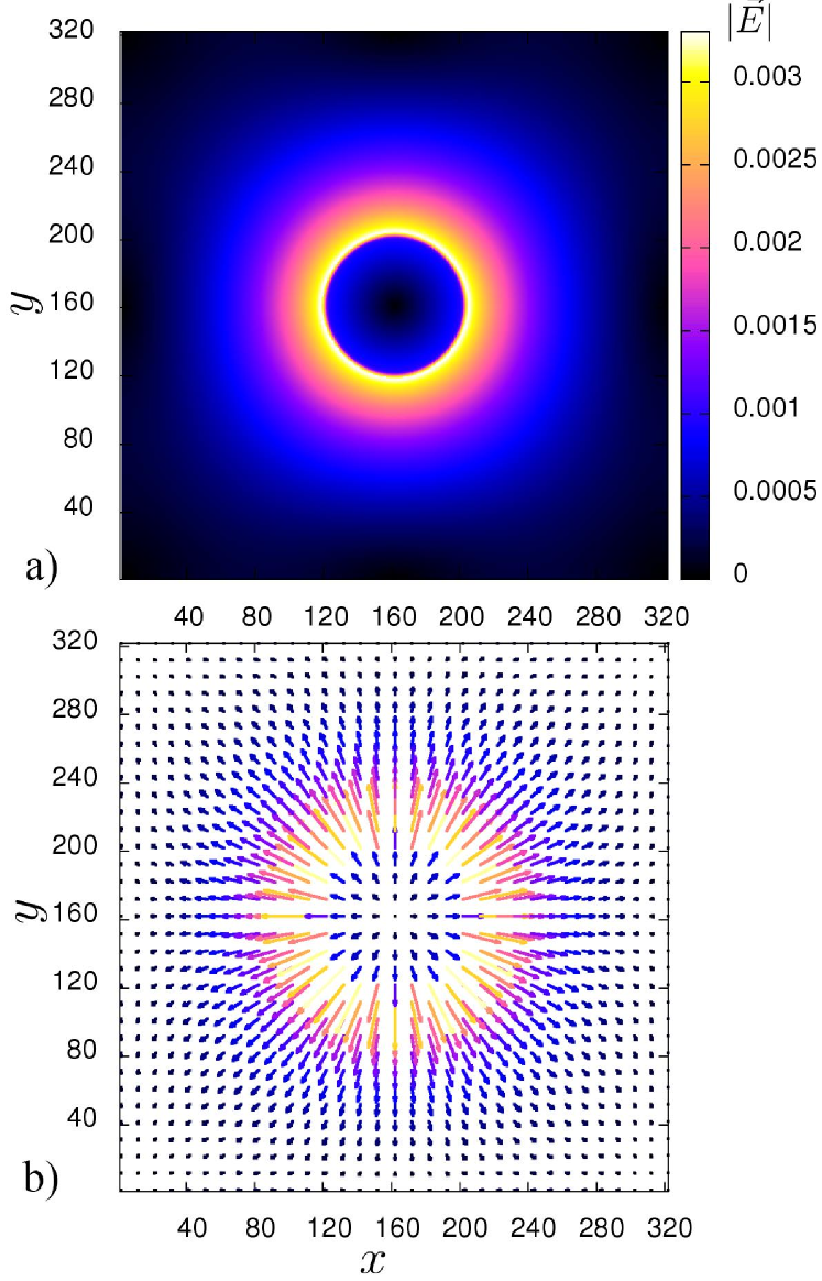
Figure 1: Profile of the electric field magnitude $|\vec{E}|$ (panel a), and its vectorial representation (panel b). Both quantities refer to the charged drop at rest.

It is of interest to estimate the various forces which concur to provide a stable configuration of the droplet. The mechanical balance reads as follows:

$$p_{L}+p_{el}=p_{V}+p_{cap}$$ (20)

where $p_{L}$ and $p_{V}$ are the liquid and vapour pressure, respectively, $p_{cap}=\sigma/R$ is the capillary pressure (given the surface tension $\sigma$ and the drop radius $R$), and $p_{el}$ is the repulsive electrostatic pressure. The latter can be estimated by standard considerations in electrostatics, namely:

$$p_{el}=\frac{Q_{s}\vec{E_{s}}\cdot\vec{n}}{2\pi R}$$ (21)

where $E_{s}$ is the electric field at the surface.

$$\frac{p_{el}}{p_{cap}}=\frac{Q_{s}E_{s}}{2\pi\sigma}$$ (22)

In actual numbers with $\sigma=5.8\cdot 10^{-2}$, this ratio is equal to $1/50$. This shows that electrostatic forces act as a small perturbation on top of the neutral multiphase physics.

Next, we investigate the effects of a uniform external electric field $E_{ext}$ of magnitude pointing along the $x$ axis. Using the previous configuration at the equilibrium as the starting point of our simulation, we set $E_{ext}$ at two different values equal to 0.1 and $0.5$. For each one of the two cases, we report a snapshot of the fluid density $\rho$ taken as soon as the liquid drop touches the point of coordinates (280,160) in lattice units. The set in Fig. 2 highlights the significant motion of the charged drop to the right in accordance with the direction of the electric field. In the figure, we note that a sizable change in the drop shape is present only for the case $E_{ext}=0.5$. In order to elucidate this effect, it is instructive to assess the strength of the electrostatic field in units of capillary forces, namely:

$$\tilde{E}\equiv\frac{QE_{ext}}{2\pi R}\frac{R}{\sigma}=\frac{QE_{ext}}{2\pi\sigma}$$ (23)

In actual numbers, this ratio is equal to 0.5 and 3 for the case at lower and higher $E_{ext}$, respectively. This shows that the electric force magnitude is sufficiently large to provide an alteration of its shape only in the case at higher $E_{ext}$. In particular, the shape shows an elongation towards the direction of the electric field $E_{ext}$, which results from the effect of the curvature on the surface charge.

In Fig. 3, we report the alteration of charge density due to the mean curvature term $K$ of Eq. 14. The alteration is estimated as $\delta_{q}=q-q_{K=0}$, where $q_{K=0}$ is computed with Eq. 14 with $K=0$ everywhere, corresponding to a constant surface charge model without curvature effect correction. Here, we note an accumulation of charge on the rightest part of the drop, where the mean curvature $K$ shows a maximum value equal to $5.17\cdot 10^{-2}$, which corresponds to a charge accumulation $\delta_{q}$ equal to $1\cdot 10^{-3}$, in the following denoted $\delta_{q}^{+}$. The accumulation of charge is counterbalanced by a negative charge $\delta_{q}^{-}$ distributed over the almost straight surface part of the drop (just behind the rightest protrusion in Fig. 3). Both partial charges $\delta_{q}^{+}$ and $\delta_{q}^{-}$ favour the presence of a protrusion in the drop shape. In order to analyze this effect, we report in Fig. 4 the mean curvature computed at the same time $t=1250\delta t$ for two simulations, both at $E_{ext}=0.5$ differing for the inclusion of the curvature effects in the constant surface charge model of Eq. 14. Even though the circular shape of the drop is deformed by the external electric field in both cases, the curvature effects increase the protrusion on the drop shape (see Fig. 4 panel b). Further, the charge differences provide a shift in the electric force acting on the drop surface, the effect of which accumulates in time, so that the alteration in the drop shape increases in time.

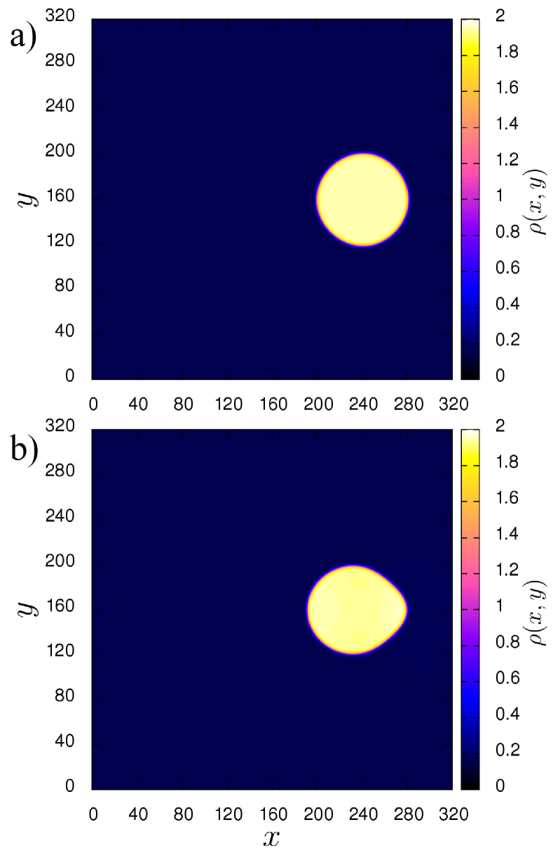
Figure 2: Two snapshots of density $\rho$ for a charged drop under an external electric field $E_{ext}$ equal to $0.1$ (panel a) and $0.5$ (panel b) taken as soon as the drop reaches the point of coordinates $(280,160)$.

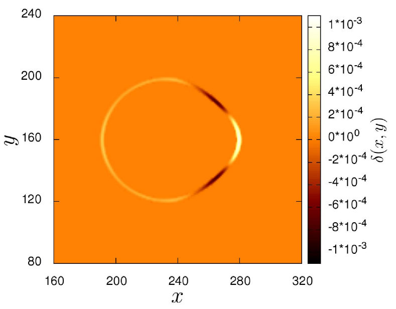
Figure 3: Alteration of charge density $q$ due to the mean curvature $K$. The alteration is estimated as $\delta_{q}=q-q_{K=0}$, where $q_{K=0}$ is computed with Eq. 14 with $K=0$ everywhere.

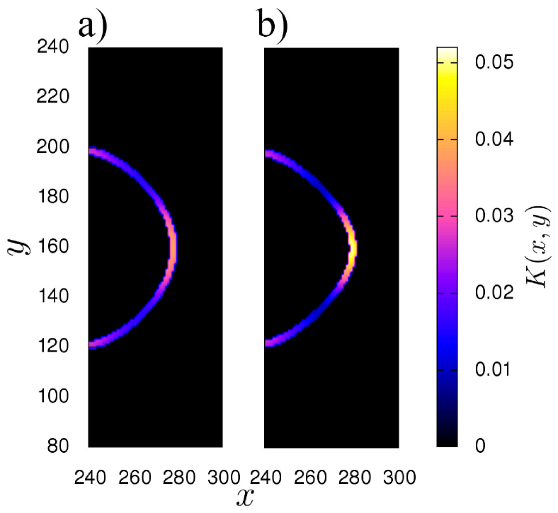
Figure 4: Mean curvature $K(x,y,)$ computed at the same time $t=1250\;\delta t$ with same surface charge $Q_{s}$ at $E_{ext}=0.5$ with two constant surface charge models: without the curvature effect (panel a), and with the curvature effect (panel b).

III.2 Charged multiphase jet in electrospinning setup

We set up a system modelling the electrospinning process, containing a charged Shan-Chen fluid. The system is a mesh made of 320 x 320 nodes (see Fig. 5). The system geometry presents, on the left side, a nozzle of diameter $D=40$, providing an initial jet radius $a_{0}=20$, that reproduces the needle of the actual electrospinning apparatus where the charged fluid is injected, while on the up and bottom sides we impose the bounce back boundary condition. As a consequence, the system is open with the inlet nodes located inside (left side) the nozzle (at $x=1$). Similarly, we set outlet nodes on the right side (at $x=320$) where the jet will impinge under the effect of the external electric field. Such electric field is chosen to mimic the potential difference that is normally applied between the nozzle and a conductive collector in the real electrospinning setup Montinaro et al. (2015). The computational setup is quite sensitive to the choice of the simulation parameters, and numerical stability has to be guaranteed by finely tuning several parameters, in particular: the density and velocity of inlet and outlet nodes, the Shan-Chen coupling constants of fluid-fluid and fluid-wall interactions, the charge constant and the magnitude of the external electric field. After preliminary simulations, we obtain a consistent set of parameters that guarantees a stable and well-shaped charged jet ejected from the nozzle.

The initial density of the two phases is $2.0$ and $0.16$ for the liquid and gaseous phase, respectively. The initial configuration consists of the liquid phase filling the inner space of nozzle with a liquid drop just outside the needle (see Fig. 5 panel a). All remaining fluid nodes are initialized to gaseous density.

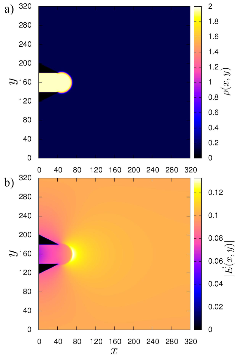
Figure 5: In panel a, the density distribution $\rho$ of the initial configuration for the electrospinning setup. In panel b, the electric field magnitude $|\vec{E}|$.

Both the Shan-Chen constants for the fluid-fluid $G$ and fluid-wall $G_{w}$ interaction are set to $-5$. As in the previous section, for the resolution of the Poisson equation, a uniform negative charge is added to the system in order to counterbalance the positive charge and obtain a system with net charge zero. Further, we impose Dirichlet boundary condition in the following form: we impose the electric potential $\phi_{l}=0$ on the left side ($x=0$), while the electric potential on the right side ($x=321$) was set equal to $\phi_{r}=-32.2$, providing a background electric field $E_{back}=(\phi_{r}-\phi_{l})/322$, which is imposed between the two opposite sides (left-right) of the system. On the upper and bottom sides, the Dirichlet boundary conditions are set equal to the $\phi_{u}(x)=\phi_{b}(x)=x(\phi_{r}-\phi_{l})/322$. Note that the last condition is equivalent to impose an electric field $\vec{E}$ of magnitude $0.1$ oriented along the x-axis.

Since in a typical electrospinning setup the liquid phase is always connected to a generator addressing a charge, it is reasonable to assume that, whenever the stretching of the liquid jet increases the jet interface, extra charge rapidly reaches the liquid boundary in order preserve the value of charge surface density. As a consequence, the charge conservation condition cannot be applied (the liquid jet is not insulated). Instead, we assume the conservation condition of the surface charge density value for the same mean curvature, so that Eq. 14 is rewritten as

$$q(\vec{r})=\xi_{b}\rho(\vec{r})\,\theta(\rho(\vec{r});\rho_{0})+\xi_{s}|\nabla\rho(\vec{r})|^{2}[1+(K/K_{d})^{\frac{1}{4}}],$$ (24)

where we have adopted a similar condition also for the bulk charge term, being $\xi_{b}$ and $\xi_{s}$ two proportionality constants, in the following taken equal to $1\cdot 10^{-4}$ and $6\cdot 10^{-2}$, respectively. Note that the two proportionality constants were tuned in order to obtain a mean ratio $Q_{s}/Q_{b}$ between the surface and bulk charge close to the target value 10, as in the previous case.

At the inlet, we set the fluid velocity in accordance with the Poiseuille velocity profile, while the density is set to $2.0$. In particular, at each time step, we compute the mean velocity of the fluid inside the nozzle, then we used this value to set up the Poiseuille profile. As a consequence, the velocities at the inlet nodes are not fixed but can change during the simulation according to the actual mean velocity measured inside the nozzle. The outlet nodes (on the right edge) are put in contact with a gas reservoir with $\rho=0.16$, so that the liquid exits by diffusion/advection.

We run three different simulations, all starting from the same initial configuration. In the first simulation the liquid is Newtonian with kinematic viscosity $\nu=1/6$, in the following denoted $case\;1$. In the other two, we employ the Carreau model (see Subsec. II.1) with zero shear kinematic viscosity $\nu_{0}=1/6$, and infinite viscosity $\nu_{\infty}=0.001$. The flow index $n$ is taken equal to 0.75, and 0.5, for the case labeled $b$, and $c$, respectively, while the relaxation time $\lambda$ was set equal to $1000$ for all the two last cases.

The internal electric field computed by the Poisson solver (see Section 2) is computed on-the-fly during the simulation. In panel b of Fig. 5 we report the electric field magnitude $|\vec{E}|$ for the initial configuration. Here, we note a maximum value of $|\vec{E}|$ close to the drop interface, which is due to the higher surface charge density. Further, a lower value of $|\vec{E}|$ is observed in the nozzle as a consequence of the larger dielectric constant $\varepsilon\simeq 3$ in the liquid phase (versus $\varepsilon\simeq 1$ in the gaseous phase).

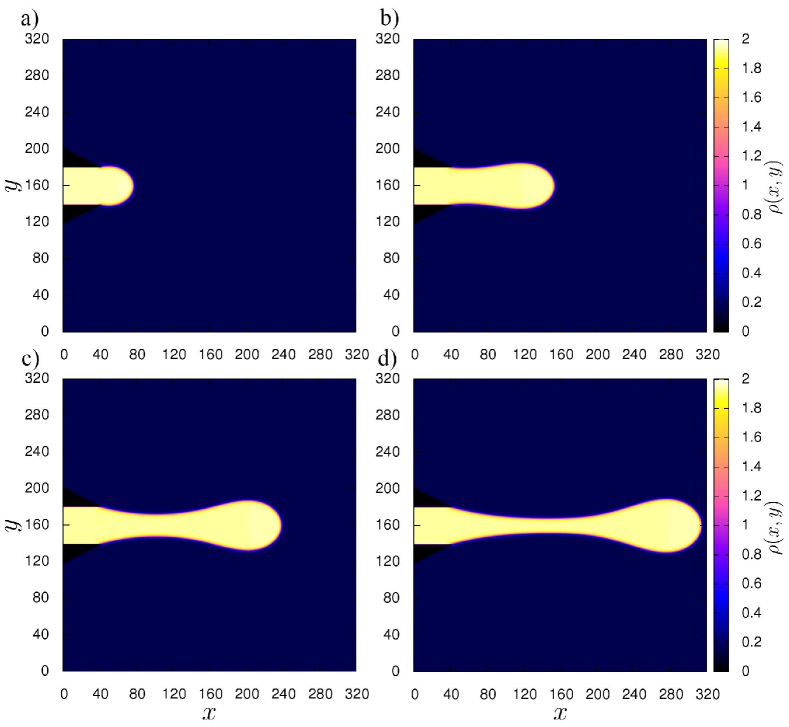
Figure 6: Series of snapshots of the fluid density $\rho$ for the electrospinning simulation $case\;b$ with index flow $n=0.75$ and relaxation time $\lambda=1000$ taken at timesteps 600(a), 5000(b), 7500(d), and 8800(d).

We now report in Fig. 6 several snapshots taken over the time evolution of the system labelled $case\;b$. In all the cases, we observe the formation of a liquid charged jet, which is ejected from the nozzle. Further, we show in Fig. 7 the velocity component $u_{x}$ measured at the extreme (rightest) point of the drop surface versus time $t$. Here, for all cases under investigation, we note that the velocity trend show the presence of a quasi-stationary point (see Fig. 6 panel a), where the viscous forces balances the external electric force in agreement with previous theoretical investigations Lauricella et al. (2015b, c, 2017); Reneker et al. (2000). In particular, such quasi-stationary point is dependent on the rheology via the viscous stress, since a different viscosity alters the balance point with the electric forces, providing a time shift of such regime. Indeed, the simulation $case\;c$ reaches the quasi-stationary condition in a shorter time (as shown in Fig. 7), since the viscous stress is weaker in sustaining the expanding electrostatic pressure in the liquid phase.

After the jet touches the collector, the jet shape fluctuates around a mean profile, providing a stationary regime. In particular, at this stage the jet shows a hyperbolic profile (see Fig. 8 panel b) which appears to be in qualitative agreement with the characteristic shape of the jet experimentally observed close to the injecting nozzle by the Rafailovich and Zussman groups Greenfeld et al. (2011) (see Fig. 8 panel a) and in consistency with previous theoretical results on the jet conical shape Reznik and Zussman (2010); Feng (2003); Higuera (2003); Hohman et al. (2001b); Hartman et al. (1999); Cherney (1999).

In Fig. 9, the effects of the local charge density and the Carreau model terms in the present ELBM are investigated. Here, we note that the jet diameter is quite sensitive to the inclusion of such effects. In particular, we observe a larger jet diameter (see right panel of Fig. 9), whenever these terms are not included in the model, showing a model failure in minimizing the jet width.

To better compare our results with experimental data from the literature, we report the Ohnesorge number, which describes the inertial, elastic and the capillary force balance. Similarly, we exploit the Deborah number, which relates the elastic stress relaxation time to the Rayleigh timescale for the inertial-capillary breakup of an inviscid jet.

In the context of the electrospinning process Arinstein (2017), the Ohnesorge and Deborah numbers are

$$Oh=\nu_{0}\sqrt{\frac{\rho}{\sigma a_{0}}},$$

$$De=\lambda\sqrt{\frac{\sigma}{\rho a^{3}_{0}}},$$ (25)

where $\rho$ is the mass density of the jet, $\sigma$ is the surface tension, $\nu_{0}$ is the zero shear kinematic viscosity, $\lambda$ is the relaxation time (see Subsec. II.1), and $a_{0}$ is the initial radius of the jet.

In our simulation, we estimate $Oh\approx 0.22$, and $De\approx 1.93$ for the Ohnesorge and Deborah number, respectively, while these two dimensionless numbers are in the value ranges $Oh\approx 0.1\--5.0$ and $De\approx 0.1\--30$ for a typical electrospinning scenario Thompson et al. (2007); Christanti and Walker (2001).

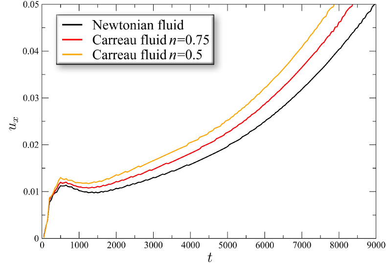
Figure 7: Velocity component $u_{x}$ registered at the extreme point (rightest point) of the drop surface versus time for all the three cases under investigation.

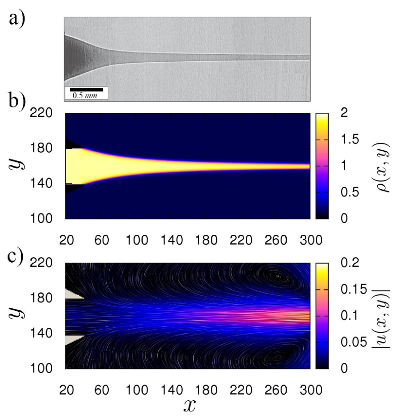
Figure 8: In panel (a), a rectilinear section of a jet in an electrospinning experiment of a solution of 5 wt% polyethylene oxide in water. Figure adapted with permission from Ref. Greenfeld et al. (2011). Copyrighted by the American Physical Society. In panel (b), a snapshot of the fluid density $\rho$ in the stationary regime after the jet has touched the right side of the simulation box in the $case\;b$. In panel (c), the corresponding velocity field magnitude $|u(x,y)|$ and the LIC representation of the velocity field.

In order to characterize the stationary regime, we report the mean values of several observables measured at the inlet. We take as a reference point the Cartesian coordinate $(x=1,z=160)$, which corresponds to the centre of the nozzle diameter. Here, we measure the velocity along $\vec{x}$ equal to $2.8\cdot 10^{-2}$ , $5.3\cdot 10^{-2}$, and $6.1\cdot 10^{-2}$ in lattice units, for the cases labeled $a$, $b$, and $c$, respectively. Further, we observe in all the three cases almost the same values in the electric field along $\vec{x}$ equal to $5\cdot 10^{-2}$ in lattice units, so we explain the velocity trend as a consequence of the lower viscosity depending on the different rheology in the three cases.

In particular, we observe a drag effect that is not depending on the local kinematic viscosity value at the inlet ($\nu_{inlet}\approx 1/6$ in all the three cases). Instead, this is due to the lower viscous force acting along the jet path outside the nozzle (as shown in panel b of Fig. 10).

Figure 9: Two sections of the jet profile $\rho(x,y)$ at timestep 10000 for the case $b$ (left panel 1), and for a simulation without the local charge density and the Carreau model terms included in the ELBM (right panel 2).

In order to characterize the stationary regime, we report in panel c of Fig. 8 the magnitude of the velocity field, and the line integral convolution (LIC) visualization technique Cabral and Leedom (1993), highlighting the fine details of the flow field. As expected, we observe a higher value of $u(x,z)$ along the jet towards the collector. In particular, we analyze the profile of the velocity in a jet cross section along what is generally observed in the experimental process.

We investigate the effect of pseudoplastic rheology on the stress tensor $\mathbf{\Pi}$. In panel a of Fig. 10 we report the mean value of the stress $\Pi$ measured along the central axis of the jet $y=160$, and averaged over a time interval of $15000$ steps in the stationary regime for the three cases under investigation.

For all cases shown in Fig. 10, we observe the presence of a drift in the $\mathbf{\Pi}$ profile starting from $x=240$. This is mainly due to the larger magnitude of the external electric force, which is originated by an increase in the surface-to-volume ratio. Since in a leaky dielectric the charge density lies mainly on the surface, such increase in the surface-to-volume ratio provides a growth of the charge-to-mass ratio. As a consequence, the jet undergoes a further stretching.

In Fig. 10, we also note a decreasing trend of the stress $\mathbf{\Pi}$ by increasing the pseudoplasticity of the fluid (decreasing the flow index $n$). Nonetheless, we observe a small shift in the stress magnitude. This is essentially due to the low value of relaxation time $\lambda$ in the Carreau model adopted in our simulation, which provides a small decrease in the kinematic viscosity $\nu$. In order to clarify this point, we report in panel b of Fig. 10 the mean value of the kinematic viscosity $<\nu>$ again assessed along the central axis of the jet $y=160$, and averaged over the stationary regime time, where we observe a small decrease of $<\nu>$ along the stretching direction as a function of the pseudoplastic behavior in the fluid. These results look promising, and we plan to investigate systematically the effect of the rheological parameters on the jet dynamics in a future work.

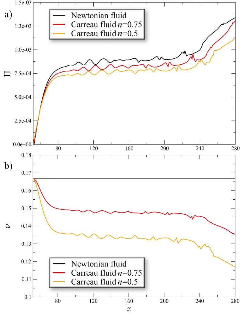
Figure 10: In panel (a), the mean value of the stress $\Pi$ computed as matrix 2-norm $<||\mathbf{\Pi}||_{2}>_{t}$ of the stress tensor measured along the central axis of the jet $y=160$ averaged over a time interval of $15000$ steps. In panel (b), the mean value of the kinematic viscosity $\nu$ computed with Eq. 19 along the central axis of the jet $y=160$, and averaged over a time interval of $15000$ steps.

IV Summary

Summarizing, we developed a Shan-Chen model for charged leaky dielectric fluids mainly aimed in modelling the electrospinning process. The curvature effects on the charged surface were included in our theoretical treatment, and we generalized the model to non-Newtonian flows in order to account for the peculiar rheological behaviour. Different scenarios were investigated to test the model. We initially investigated the effect of strong electric fields on the droplet shape evolution. We also probed the jet formation under electrospinning-like conditions, obtaining a good agreement with both experimental results and previous theoretical works present in literature. At first glance, the pseudoplastic behaviour alters the jet dynamics, although a more systematic investigation requires an extensive test of the rheological parameters. Work along these lines is currently underway.

The preliminary applications of the presented ELBM look promising, although more systematic numerical investigations, as well as theoretical analysis, need to be undertaken. Nonetheless, the actual effort can be regarded as a significant forward step to extend the applicability of the ELBM to the context of electrospinning systems, providing a useful computational tool in the completion of the others presently available in the literature.

Appendix A Units Conversion Table

Symbol	Definition	2-d lattice units	3-d cgs units
$\rho$	Mass density	$1\;\Delta m\,\Delta l^{-2}$	$0.5\;\text{g}\,\text{cm}^{-3}$
$u$	Velocity	$1\;\Delta l\,\Delta t^{-1}$	$1200\;\text{cm}\,\text{s}^{-1}$
$\nu$	Kinematic viscosity	$1\;\Delta l^{2}\,\Delta t^{-1}$	$1.2\;\text{cm}^{2}\,\text{s}^{-1}$
$q$	Charge	$1\;\Delta l^{3/2}\,\Delta m^{1/2}\,\Delta t^{-1}$	$8.5\cdot 10^{-4}\,\text{statC}$
$E$	Electric field	$1\;\Delta l^{-1/2}\,\Delta m^{1/2}\,\Delta t^{-1}$	$848.5\;\text{statV}\,\text{cm}^{-1}$
$\phi$	Electric potential	$1\;\Delta l^{1/2}\,\Delta m^{1/2}\,\Delta t^{-1}$	$8.485\cdot 10^{-1}\;\text{statV}$
$\varepsilon$	Relative permittivity	$-$	$-$
$a_{0}$	Initial jet radius	$1\;\Delta l$	$10^{-3}\text{cm}$
$K$	Mean curvature	$1\;\Delta l^{-1}$	$1000\;\text{cm}^{-1}$
$\dot{\gamma}$	Shear rate	$1\;\Delta t^{-1}$	$1.2\cdot 10^{6}\,\text{s}^{-1}$
$\Pi$	Stress	$1\;\Delta m\,\Delta t^{-2}$	$7.2\cdot 10^{5}\,\text{g}\,\text{cm}^{-1}\,\text{s}^{-2}$
$\lambda$	Relaxation time	$1\;\Delta t$	$8.3\cdot 10^{-7}\;\text{s}$
$n$	Index flow	$-$	$-$
$p$	Pressure	$1\;\Delta m\,\Delta t^{-2}$	$7.2\cdot 10^{5}\,\text{g}\,\text{cm}^{-1}\,\text{s}^{-2}$
$\sigma$	Surface tension	$1\;\Delta l\,\Delta m\,\Delta t^{-2}$	$720\;\text{g}\,\text{s}^{-2}$

Table 1: Symbols employed in order of appearance, their definitions, relative dimensions in 2-d lattice units, and conversion values in 3-d Gaussian centimetre-gram-second (cgs) system of units. The conversion to 3-d dimension units is obtained by multiplying the 2-d square area $\Delta l^{2}$ for an extra node $\Delta l$ along the z-axis. Note that $\Delta m$ denotes the mass unit equal to $5\cdot 10^{-10}$ g (water density), $\Delta l$ the length unit equal to $10^{-3}\text{cm}$, and time step $\Delta t$ is the time unit equal to $8.3\cdot 10^{-7}$ s. The last number was tuned in order to set the kinematic viscosity $\nu=1/6\;\Delta l^{2}\,\Delta t^{-1}=0.2\;\text{cm}^{2}\text{s}^{-1}$ in similarity with the viscosity value adopted in the Lagrangian model of Ref. Lauricella et al. (2015a).

References

- Yarin et al. (2014) A. L. Yarin, B. Pourdeyhimi, and S. Ramakrishna, Fundamentals and applications of micro-and nanofibers (Cambridge University Press, 2014).
- Wendorff et al. (2012) J. H. Wendorff, S. Agarwal, and A. Greiner, Electrospinning: materials, processing, and applications (John Wiley & Sons, 2012).
- Pisignano (2013) D. Pisignano, Polymer Nanofibers: Building Blocks for Nanotechnology, Vol. 29 (Royal Society of Chemistry, 2013).
- Frenot and Chronakis (2003) A. Frenot and I. S. Chronakis, Current opinion in colloid & interface science 8, 64 (2003).
- Huang et al. (2003) Z.-M. Huang, Y.-Z. Zhang, M. Kotaki, and S. Ramakrishna, Composites science and technology 63, 2223 (2003).
- Li et al. (2004) D. Li, Y. Wang, and Y. Xia, Advanced Materials 16, 361 (2004).
- Greiner and Wendorff (2007) A. Greiner and J. H. Wendorff, Angewandte Chemie International Edition 46, 5670 (2007).
- Carroll et al. (2008) C. P. Carroll, E. Zhmayev, V. Kalra, Y. L. Joo, et al., Korea-Australia Rheology Journal 20, 153 (2008).
- Persano et al. (2013) L. Persano, A. Camposeo, C. Tekmen, and D. Pisignano, Macromolecular Materials and Engineering 298, 504 (2013).
- Reneker et al. (2000) D. H. Reneker, A. L. Yarin, H. Fong, and S. Koombhongse, Journal of Applied physics 87, 4531 (2000).
- Feng (2003) J. Feng, Journal of Non-Newtonian Fluid Mechanics 116, 55 (2003).
- Lauricella et al. (2015a) M. Lauricella, G. Pontrelli, I. Coluzza, D. Pisignano, and S. Succi, Computer Physics Communications 197, 227 (2015a).
- Lauricella et al. (2016a) M. Lauricella, G. Pontrelli, D. Pisignano, and S. Succi, Journal of Computational Science 17, 325 (2016a).
- Lauricella et al. (2016b) M. Lauricella, D. Pisignano, and S. Succi, The journal of physical chemistry. A 120, 4884 (2016b).
- Ganan-Calvo (1997) A. M. Ganan-Calvo, Journal of Fluid Mechanics 335, 165 (1997).
- Hohman et al. (2001a) M. M. Hohman, M. Shin, G. Rutledge, and M. P. Brenner, Physics of fluids 13, 2201 (2001a).
- Yarin et al. (2001a) A. L. Yarin, S. Koombhongse, and D. H. Reneker, Journal of applied physics 89, 3018 (2001a).
- Li and Kwok (2003) B. Li and D. Y. Kwok, Physical review letters 90, 124502 (2003).
- Kupershtokh and Medvedev (2006) A. Kupershtokh and D. Medvedev, Journal of electrostatics 64, 581 (2006).
- Huang et al. (2007) W. Huang, Y. Li, and Q. Liu, Chinese Science Bulletin 52, 3319 (2007).
- Gong et al. (2010) S. Gong, P. Cheng, and X. Quan, International Journal of Heat and Mass Transfer 53, 5863 (2010).
- Medvedev (2010) D. Medvedev, Procedia Computer Science 1, 811 (2010).
- Bararnia and Ganji (2013) H. Bararnia and D. Ganji, Advanced Powder Technology 24, 992 (2013).
- Kupershtokh (2014) A. L. Kupershtokh, Computers & Mathematics with Applications 67, 340 (2014).
- Landau et al. (2013) L. D. Landau, J. Bell, M. Kearsley, L. Pitaevskii, E. Lifshitz, and J. Sykes, Electrodynamics of continuous media, Vol. 8 (elsevier, 2013).
- Taylor (1964) G. Taylor, Proceedings of the Royal Society of London A: Mathematical, Physical and Engineering Sciences, 280, 383 (1964).
- Taylor (1966) G. Taylor, Proceedings of the Royal Society of London A: Mathematical, Physical and Engineering Sciences, 291, 159 (1966).
- Taylor (1969) G. Taylor, Proceedings of the Royal Society of London A: Mathematical, Physical and Engineering Sciences, 313, 453 (1969).
- Saville (1997) D. Saville, Annual review of fluid mechanics 29, 27 (1997).
- Karlin et al. (1999) I. Karlin, A. Ferrante, and H. C. Öttinger, EPL (Europhysics Letters) 47, 182 (1999).
- Hua et al. (2008) J. Hua, L. K. Lim, and C.-H. Wang, Physics of Fluids 20, 113302 (2008).
- Li et al. (2011) Z.-T. Li, G.-J. Li, H.-B. Huang, and X.-Y. Lu, International Journal of Modern Physics C 22, 729 (2011).
- Ansumali and Karlin (2002) S. Ansumali and I. V. Karlin, Physical Review E 65, 056312 (2002).
- Chikatamarla et al. (2006) S. S. Chikatamarla, S. Ansumali, and I. V. Karlin, Physical review letters 97, 010201 (2006).
- Dorschner et al. (2016) B. Dorschner, F. Bösch, S. S. Chikatamarla, K. Boulouchos, and I. V. Karlin, Journal of Fluid Mechanics 801, 623 (2016).
- Ansumali et al. (2003) S. Ansumali, I. V. Karlin, and H. C. Öttinger, EPL (Europhysics Letters) 63, 798 (2003).
- Kupershtokh et al. (2009) A. Kupershtokh, D. Medvedev, and D. Karpov, Computers & Mathematics with Applications 58, 965 (2009).
- Quarteroni and Valli (2008) A. Quarteroni and A. Valli, Numerical approximation of partial differential equations, Vol. 23 (Springer Science & Business Media, 2008).
- Gañán-Calvo (2004) A. M. Gañán-Calvo, Journal of fluid mechanics 507, 203 (2004).
- McAllister (1990) I. McAllister, Journal of Physics D: Applied Physics 23, 359 (1990).
- Spencer et al. (2010) T. J. Spencer, I. Halliday, and C. M. Care, Physical Review E 82, 066701 (2010).
- Yarin et al. (2001b) A. L. Yarin, S. Koombhongse, and D. H. Reneker, Journal of applied physics 90, 4836 (2001b).
- Chikatamarla et al. (2015) A. Mazloomi M,S. S. Chikatamarla, I. V. Karlin, Physical review letters 114, 174502 (2015).
- Huang et al. (2015) H. Huang, M. Sukop, and X. Lu, Multiphase lattice Boltzmann methods: Theory and application (John Wiley & Sons, 2015).
- Falcucci et al. (2010) G. Falcucci, S. Ubertini, and S. Succi, Soft Matter 6, 4357 (2010).
- Shan and Chen (1993) X. Shan and H. Chen, Physical Review E 47, 1815 (1993).
- Pontrelli et al. (2009) G. Pontrelli, S. Ubertini, and S. Succi, Journal of Statistical Mechanics: Theory and Experiment 2009, P06005 (2009).
- Gabbanelli et al. (2005) S. Gabbanelli, G. Drazer, and J. Koplik, Physical review E 72, 046312 (2005).
- Aharonov and Rothman (1993) E. Aharonov and D. H. Rothman, Geophysical Research Letters 20, 679 (1993).
- Ouared and Chopard (2005) R. Ouared and B. Chopard, Journal of statistical physics 121, 209 (2005).
- Agarwal et al. (2016) S. Agarwal, M. Burgard, A. Greiner, and J. Wendorff, Electrospinning: A Practical Guide to Nanofibers (Walter de Gruyter GmbH & Co KG, 2016).
- Johnson (2016) R. W. Johnson, Handbook of fluid dynamics (Crc Press, 2016).
- Montinaro et al. (2015) M. Montinaro, V. Fasano, M. Moffa, A. Camposeo, L. Persano, M. Lauricella, S. Succi, and D. Pisignano, Soft matter 11, 3424 (2015).
- Lauricella et al. (2015b) M. Lauricella, G. Pontrelli, D. Pisignano, and S. Succi, Molecular Physics 113, 2435 (2015b).
- Lauricella et al. (2015c) M. Lauricella, G. Pontrelli, I. Coluzza, D. Pisignano, and S. Succi, Mechanics Research Communications 69, 97 (2015c).
- Lauricella et al. (2017) M. Lauricella, F. Cipolletta, G. Pontrelli, D. Pisignano, and S. Succi, Physics of Fluids 29, 082003 (2017).
- Greenfeld et al. (2011) I. Greenfeld, A. Arinstein, K. Fezzaa, M. H. Rafailovich, and E. Zussman, Physical Review E 84, 041806 (2011).
- Reznik and Zussman (2010) S. N. Reznik and E. Zussman, Physical Review E 81, 026313 (2010).
- Higuera (2003) F. Higuera, Journal of Fluid Mechanics 484, 303 (2003).
- Hohman et al. (2001b) M. M. Hohman, M. Shin, G. Rutledge, and M. P. Brenner, Physics of fluids 13, 2221 (2001b).
- Hartman et al. (1999) R. P. A. Hartman, D. Brunner, D. Camelot, J. Marijnissen, and B. Scarlett, Journal of Aerosol science 30, 823 (1999).
- Cherney (1999) L. T. Cherney, Journal of Fluid Mechanics 378, 167 (1999).
- Arinstein (2017) A. Arinstein, Electrospun Polymer Nanofibers: A physicist’s point of view (CRC Press, 2017).
- Thompson et al. (2007) C. Thompson, G. G. Chase, A. Yarin, and D. Reneker, Polymer 48, 6913 (2007).
- Christanti and Walker (2001) Y. Christanti and L. M. Walker, Journal of Non-Newtonian Fluid Mechanics 100, 9 (2001).
- Cabral and Leedom (1993) B. Cabral and L. C. Leedom, in Proceedings of the 20th annual conference on Computer graphics and interactive techniques (ACM, 1993) pp. 263–270.