Cumulant-based formulation of higher-order fluorescence correlation spectroscopy
Abstract
Extended derivations regarding the cumulant-based formulation of higher-order fluorescence correlation spectroscopy (FCS) are presented. First, we review multivariate cumulants and their relation to photon counting distributions in single and multi-detector experiments. Then we derive the factorized correlation functions which describe system of diffusing and reacting molecules using two independent approaches. Finally, we calculate the variance of these correlation functions up to the fourth order.
1 Introduction
Fluorescence correlation spectroscopy (FCS) is a powerful technique for a time-resolved analysis of reaction, diffusion, and flow properties of individual fluorescent molecules moving through a laser-illuminated probe region[4, 7, 16]. Conventional FCS is based on second-order correlation functions only, hence insufficient for measuring the parameters which describe molecular reactions or mixtures[1, 19] such as species populations and brightness values and the kinetic rate constants. Higher-order correlation functions can provide the necessary information for a complete measurement of the underlying reaction or mixture parameters. Previous work to define higher-order correlations based on higher moments of the fluorescence signal lead to complex expressions for mixtures of diffusing molecules[11, 13, 12], thus no extension of such approach to include reactions has been proposed. More recently, a formulation based on the cumulants of the fluorescence intensity or the factorial cumulants of the detected photon counts has been published, which results in correlation functions incorporating reaction and diffusion properties in a simple factorized form[9]. To experimentally apply the technique to the study of fast molecular kinetics, difficulties due to shot noise and detector artifacts have been recently overcome[1, 2].
Theoretically, the formulation of correlation functions based on multi-variate cumulants utilizes a variety of concepts not commonly covered in the available literature on FCS. A detailed description of the theoretical basis and derivations can make the underlying work for some earlier publications[1, 2, 9] more accessible. This document has been produced with such purpose in mind, and presents no further results and findings.
The material in this document appears in developmental order. That is, some introductory content is presented first and a continuous forward flow of reading is assumed. However, informed reader may skip to the desired section. Effort has been made to facilitate independent reading of this document by including the necessary preliminary information, derivations, and relations.
2 Mathematical introduction and notation
In this section we review the definitions, notation, and relations between multivariate moments, central moments, cumulants, and their factorial counterparts. For a more thorough treatment, the reader may refer to [3, 15].
In what follows, we use to denote and use to denote . Also, we will use the differential operators
We will occasionally exchange the order of product and summation in the following way:
For simplicity, we assume the moments, etc. exist and the expansions converge.
2.1 (Central) moments and cumulants
Let be a multivariate random vector. For the th moment of is defined as
where denotes the expectation operator. In particular,
where has only the th element equal to 1.
The th central moment of is defined as
| (1) |
We denote the moment generating function of by
| (2) | ||||
and the central moment generating function of by
| (3) | ||||
| (4) |
where
and is the th central moment (or moment about the mean) of .
The cumulant generating function of is defined as
| (5) | ||||
| (6) |
which also defines , the th cumulant of , through multiple differentiation of
One can proceed to substitute the expansions (6) and (4) into relation (5), or into , then expand the or the function and set the terms of equal order in equal to each other to obtain the relationship between the cumulants and the moments . Then setting all the first order moments equal to zero in the resultant expressions and dropping the primes will yield the relations between the cumulants and the central moments . Alternatively, one can write, using (3),
| (7) |
and expand to obtain the relations between and . The central moments, and therefore , do not depend on the mean values . In other words, , thus terms of individual do not appear in the expansion of . Thus (7) immediately shows that the first cumulant of each is equal to its mean,
Also, all higher order central moments are independent of mean in the sense that they are invariant under translation of origin. Therefore (7) shows that all higher order cumulants are also independent of mean, i.e. invariant under change of origin.
Cumulants share the described invariance property with central moments. However, cumulants also have another property which makes them unique: Each cumulant of a sum of independent random variables is equal to the sum of the corresponding cumulants of those random variables. To see this, consider two independent random vectors and . Directly from definition (2) we have for the moment generating function of their sum,
| (indep. , ) | ||||
Now from (5)
Expanding and setting the coefficients equal we get:
| (8) |
This property makes cumulants particularly useful in the study of single molecules in solution, where each molecule can be considered as an independent emitter of photons. Fluorescence Cumulant Analysis (FCA) [10, 18] and Higher Order Fluorescence Correlation Spectroscopy [9] are examples of such applications.
To obtain relations between multivariate cumulants and central moments, it will be more convenient to use recursive formulas rather than the expansion method mentioned above. Such formulas are obtained through successive differentiation of the relevant moment generating function, as presented by Balakrishnan et al [3]. For let us find the central moment in terms of the cumulants of order and less (i.e. for all ), and the central moments of order and less:
| (9) |
It is easy to see for multiple derivatives of a product
From there,
Applying this to (9) with and we obtain
| (10) |
We write the first few relations up to a total order of four. For a univariate distribution, we have directly from definition (1):
Then from (5)
The recursive formula (10) now generates the rest:
which equals zero, thus
Again from (10),
And for :
For example,
conversely,
and so forth.
For a bivariate distribution, we have directly from the definitions, (1):
and from (5):
The recursive formula (10) now yields
which vanishes, thus
also follows the univariate relation:
As evident from basic definitions, , , and are identical to univariate cases and follow their relations:
and so forth.
A useful symmetry property also follows from the definitions: exchanging the subscripts in any valid relation between s and s will produce a valid relation. Thus we can find the expression for (or ) from the that of (or ).
Once again our recursive formula (10) can be applied:
By symmetry,
In general, for ,
For example,
Conversely,
As other examples,
which could also be obtained by swapping the subscripts. Conversely,
and so forth.
2.2 Factorial moments and factorial cumulants
The tools developed in this section are particularly useful for discreet random variables. In what follows, suppose can take only non-negative integer values .
The th (descending) factorial moment of is defined as
where
denotes the th (falling) factorial power of . Because , for . The constants are called the Stirling numbers of the first kind. Conversely,
defines the Stirling numbers of the second kind, .
Thus we have
| (11) |
which gives factorial moments in terms of moments. Similarly,
| (12) |
giving moments in terms of factorial moments.
The probability generating function of is defined as
| (13) | ||||
where
is the probability that takes the value .
Now we define through a change of variable in the probability generating function, :
| (14) | ||||
| Since for | ||||
| Now we can switch the summation order | ||||
Therefore, is in fact the factorial moment generating function of .
The factorial cumulant generating function of is then defined as
| (15) | ||||
which also defines , the th factorial cumulant of , through multiple differentiation of :
As with ordinary moments and cumulants, one can proceed to expand and in (15) and compare term by term to obtain the relations between and . This procedure is identical to that of finding the relations between and , noting the similarity between (15) and . Therefore the relations between factorial moments and factorial cumulants are formally similar to those between moments and cumulants, obtained in section 2.1.
It remains to determine the relations between cumulants and factorial cumulants. To this purpose, we first examine the relation between the moment generating function, , and the factorial moment generating function, , of . Using the change of variables in (13) and comparing with (2) we can write
On the other hand, (14) gives , thus we have
| (16) |
Taking the natural logarithm of both sides we also have
| (17) |
as the relation between the cumulant generating function, , and the factorial cumulant generating function, , of . Expanding both sides of (16) and equating terms of equal order in yields the relations between moments and factorial moments, which were previously found in (11) and (12) through direct use of definitions. Noting the similarity between (16) and (17), formally similar relations are then obtained through expansion of (17) between cumulants and factorial cumulants:
It will be instructive to actually expand (16) and equate the corresponding coefficients of on the two sides. Expanding the right hand side gives:
| while the left hand side is equal to | ||||
Therefore,
| (18) |
Let us rewrite (12) as:
| Since for and for | ||||
Comparing with (18) we get
an explicit expression for the Stirling numbers of the second kind.
We finish this section by tabulating the relations between cumulants and factorial cumulants up to 4th order for future reference.
| (23) | ||||
| (28) | ||||
| Conversely | ||||
| (32) | ||||
| (36) | ||||
3 The relation between fluorescence intensity and photon counting distributions
Consider a fluorescence detection experiment involving channels and denote the fluorescence light intensity in channel at time by . Typically, different channels consist of different detectors and/or signals at different lag times.
Let us for the time being limit our discussion to a single channel and drop the subscript in the relevant quantities. Consider a time interval (bin) of size and set the origin at its beginning: . Absorbing all efficiency parameters into , or assuming perfect efficiency, the probability of detecting a photon in the infinitesimal interval is given by . The probability of detecting no photons in the interval is given by the product of the probabilities of detecting no photons in each infinitesimal interval in that interval:
Let us also define and . For the probability of detecting exactly photons at infinitesimal intervals where is given by
Now considering various placements of subject to the condition , the probability of detecting exactly photons in the whole bin given a particular becomes
The integrand is symmetric: it has the same value at any permutation of the s. Any permutation of s in covers a separate block of the parameter space, and the integration yields the same value over each block. The union of all such blocks, or permutations of the s, covers the entire span of for all . There are blocks, therefore we have
| (37) |
Now we take the fluctuations of into account. Let denote the probability that the fluorescence intensity takes a value within an infinitesimal variation around defined over . Assuming a stationary process, binning a long experimental time and averaging a quantity over all such bins, as done in an FCS experiment, is equivalent to averaging that quantity over an ensemble of (ergodicity). The probability of detecting photons in each bin is therefore
| (38) |
where is given by (37). A more useful random variable is the integrated intensity within the bin time , defined as
| (39) |
The probability of detecting photons in the bin, (38), can be written as
where, by (37),
Thus we obtain Mandel’s formula[8]:
We can now consider the case of multiple channels, and a common bin size . The fluorescence intensities at different channels are not necessarily independent. Neither are the integrated intensities, . However, given particular the occurrence probabilities of photons in distinct channels are, by definition, independent:
| (40) | ||||
”Distinct” channels in practice can be bins (overlapping with no cross-talk, or non-overlapping) in independent detector signals, or non-overlapping bins in a single detector signal. Denoting the joint probability of integrated intensities taking the values by and integrating (40) we obtain for the joint probability of detecting photons in channel :
| (41) |
which is the multivariate form of Mandel’s formula.
To abbreviate notation, we define and using boldface symbols in our general treatment of multiple channels, to be distinguished from vectors introduced later specific to two-time correlation experiments.
Let us now examine the relations between moments (or cumulants) of and moments (or cumulants) of . The probability generating function of is
where the shorthand notation
has been used. The factorial moment generating function of is
| using Mandel’s formula, (41), | ||||
| (42) | ||||
the moment generating function of . This shows that the factorial moments of are equal to the (ordinary) moments of .
Taking the natural logarithm of (42) we also obtain:
| (43) |
That is, the factorial cumulants of are equal to the (ordinary) cumulants of .
Alternatively, we can calculate the factorial moments of directly:
| and since for | ||||
Then we can argue that the f.m.g.f. of is equal to m.g.f. of . From there, (43) and the equality of the factorial cumulants of with the corresponding cumulants of follow:
| (44) |
3.1 Two-time correlations***The content of this section is available in reference [1] and is brought here for the sake of continuity.
We can now use Equation (44) to describe the correlation functions between two lag times, and . A number of methods have been proposed due to the experimental limitations which arise from detector artifacts, namely dead-time, after-pulsing, and cross-talk. The effects of these artifacts in higher-order correlations extend to all time scales, beyond the better-known effects in second-order FCS which occur at short lag times only. Multi-detector and/or “sub-binning” approaches have been proposed to overcome these issues in higher-order FCS. These methods have been described in another article[1] along with the advantages and disadvantages of each method.
In brief, a single-detector method with no modification usually suffers most severely from detector artifacts. Earlier work tried to estimate and account for these artifacts[9, 5, 17], however, the extra modeling, approximations, and calibrations can make such analysis more complicated and less versatile. Using two or more detectors may avoid dead-time and after-pulsing artifacts, however, cross-talk between the detectors may become an issue if not experimentally prevented. Sub-binning refers to using smaller, non-overlapping intervals (sub-bins) within the larger sampling intervals (bins). The independent sub-bins virtually convert a single-detector experiment to a multi-detector one with no cross-talk issue. In a true multi-detector experiment, sub-binning also helps avoid the cross-talk artifact. Therefore, sub-binning yields artifact-free results in both single-detector and multi-detector experiments.[1]
The discussion below assumes no sub-binning. For sub-binning we can employ the multi-detector formulation without sub-binning; no separate formulation is needed.
3.1.1 Single-Detector Experiment
When only one detector is used in the experiment (without sub-binning), we can denote the fluorescence intensity at the detection point at zero lag time by and at lag time by . Take and to denote the corresponding integrated intensities over some binning time , that is
Also, and denote the number of photons detected in the corresponding bins. The random vectors , , and are then defined accordingly. Relation (44) then directly yields
| (45) |
3.1.2 Multi-Detector Experiment
We can use independent detectors (without sub-binning) to obtain correlations of order with . We assume that the beamsplitters and the detection efficiencies are adjusted such that the light intensity is equal for all detectors at any moment. Then take to denote the fluorescence light intensity arriving at any detector at lag time zero, and to denote that intensity at lag time . Correspondingly, and are defined by integration over a sampling interval (bin) of size , as in the single-detector case. The random vectors and are also defined accordingly. The photon count in the th detector during a bin is a distinct random variable for each detector, . Therefore we define the vector
| (46) |
Relation (44) directly yields
| (47) |
where has elements.
In particular, for the case of two detectors named and we have:
4 Modeling correlations for diffusing and reacting molecules
In this section we derive the relations describing higher order fluorescence correlations for molecules of a single-species which simultaneously diffuse and undergo reaction between multiple states. We assume the molecules have the same diffusion constant in all the ration states. This multi-state system reduces to a multi-species non-interacting system when the reaction rates are set to zero, with identical diffusion constant for all species assumed. A mixture of reacting and non-reacting species can also be described by setting only a subset of the reaction rates equal to zero.
Palmer and Thompson [11] defined higher-order correlations using higher-order moments of intensity. For mixtures of diffusing molecules, the moment-based definition of correlation functions leads to complex expressions that depend on lower-order correlation functions. No such expression has been proposed to include reactions of diffusing molecules due to the increased complexity of formulation. Later, Melnykov and Hall[9], following the approach developed by Müller in the study of Fluorescence Cumulant Analysis [10], presented a definition of higher-order correlations based on higher-order cumulants. In their derivation, Melnykov and Hall used the additive property of cumulants to arrive at simple factorized expressions for the cumulant-based higher-order correlation functions describing systems of diffusing molecules with reactions.
In comparison to moments, the computation of cumulants from the experimental photon stream is only slightly more complicated: moments are first computed, then converted to cumulants using tabulated relations. However, with the cumulant-based formulation, the theoretical relations which describe systems of diffusing and reacting molecules are much simpler than with the moment-based formulation. Most importantly, with the cumulant-based formulation, the expressions factorize into pure reaction and diffusion parts for systems with independent reaction and diffusion processes. This allows for the experimental removal of any dependence on the molecular detection function (MDF, defined as the combination of laser intensity distribution, collection point-spread function, and pinhole aperture[14]) and on the diffusion constant by using a reference measurement[2].
In this section, before presenting the derivation reported by Melnykov and Hall, we present an alternative derivation starting from simpler premises and use a reverse reasoning process: we start from the explicit integrals following the definition of higher-order moments, (50), and find conversion relations by only demanding simple final expressions which are factorized into reaction and diffusion parts, (77), without assuming any knowledge about cumulants, their properties, and their relation to moments. Only then, we show that such conversion relations are in general equivalent to the well-known conversion relations between moments and cumulants. We label this approach the Palmer-Thompson approach because the explicit expression of integrals using Dirac and Kronecker delta functions was inspired by the work of those authors. On the other hand, Melnykov and Hall used the well-known additive property of cumulants to directly derive the simple factorized expressions for a multi-particle system based on the moments for a single particle. While the approach by Melnykov and Hall is more concise and elegant, the Palmer-Thompson approach is more elaborate and instructive therefore it is discussed first. The two derivations are formally independent and the reader may skip to the second approach if desired (after the introductory discussion below).
Some preliminary discussion comes first. Take the random vector , where, following (39),
The general dependence of non-correlated higher moments of on the bin size, , has been studied by Wu and Müller [18] for non-interacting diffusing molecules through the introduction of “binning functions”. In this report, however, we limit our attention to the case of small bin sizes. For a short bin size over which the variations of intensity can be neglected, we have
| (48) |
which becomes exact in the limit .
Absorbing any detection efficiency factors into , we can write
| (49) |
where is the laser illumination profile normalized to its peak value, is the number of molecular states, is the brightness of state at illumination peak in counts per unit time per molecule, is the concentration of the particles in state at position and time , and is an integration volume that includes the illuminated region. can be taken to be the entire sample volume containing a fixed number of molecules, .
Therefore we have, in the limit ,
| (50) | ||||
where
| (51) | ||||
The concentration of particles in state at position at time is given by
| (52) |
where and are the state and position of the th particle at time , respectively. and denote the Kronecker and the Dirac delta functions, respectively. is the total number of molecules in the large sample volume . We will later take the limit .
Assuming a stationary (ergodic) system, the expected value of concentration of particles in state at position can be obtained by averaging over and as they vary over time:
where
| (53) | ||||
| (54) |
Here, denotes the probability that a given particle is in state and
is a uniform probability density that the particle is found anywhere in the solution. Denoting the expected number of particles in state by
we get
| (55) |
Also, assuming ergodicity,
Taking the expectation of (49) and using (55), the mean detection count rate is found to be
| (56) |
where we have defined
| (57) |
and
| (58) |
In the limit , approaches the volume of the molecular detection function (observation volume, or probe region), and approaches the average number of molecules in state in the observation volume.
Consider a single particle, for example the th one. We define and evaluate
| (59) |
For brevity, take , , , and . Then
where denotes the joint probability that the particle is at state and position at time , and at state and position at time . It can be expressed in terms of conditional probabilities,
where denotes the probability that the particle is found in state at time given it was in state at time , and is [obtained by solving linear rate equations, Appendix D]:
Similarly, the probability density function of the particle being at position at time given it was at position at time is [obtained from solving the diffusion equation]
Therefore for a single molecule we obtain
| (60) |
Next, it will be helpful to define and evaluate
| (61) |
Immediately from (59), (60), and (55) we get:
| (62) | ||||
| (63) |
Setting we have:
4.1 Palmer-Thompson approach
This method follows the work of Palmer and Thompson [11] where they directly evaluate . We have modified the notation to incorporate multiple states, and will show that this method is equivalent to the cumulant-based formulation.
Using (52) we have
We break the summation according to the following cases:
-
•
When two or more particle indices are different (at any lag time) the expectation operator of product of independent random variables factorizes. As a special case, when all particles at both lag times are different:
To justify this approximation, notice that according to (54) each term in the sum is of order . The summation on the left has exactly terms, and the right hand side, written as products of sums and expanded, has exactly terms. The sum of the extra terms on the right hand side (pertaining to two or more equal indices) is then of order . In the thermodynamic limit these extra terms become negligible and the relation becomes exact.
-
•
When two or more particles indices are the same at the same lag time, the expectation operator factorizes into products of delta functions and a single concentration. As a special case, when all particle indices at lag time are identical:
This can be justified by writing the expectation operator in the explicit form of (53) and using the change of variables for the spatial part. The discrete part is nonzero only when all indices are identical.
-
•
When two or more particle indices are the same at different lag times, the expectation operator factorizes into products of delta functions and a single propagator. As a special case, when all indices at lag time and are identical:
(64) where is defined in (61).
Let us start with calculating the simpler cases of and . We have by definition (51)
For moments of order , the summation in runs over two particle indices. Therefore, it can be broken into two cases where the two indices are either equal or not equal:
A similar result is obtained for , in a similar fashion.
For correlation of order , the summation in is also over two particle indices only, and it can be broken in a similar way:
| (65) | |||||
For order , there are three particle indices:
| and we break the sum into five categories: | ||||
| (66) | ||||
The categorization of the terms in the summation above corresponds to partitioning of a set of items. A partition of a set is defined as a set of nonempty, pairwise disjoint subsets of whose union is . There is a one-to-one correspondence between the terms in (66) and the partitions of a set of items shown in Figure 1, left.
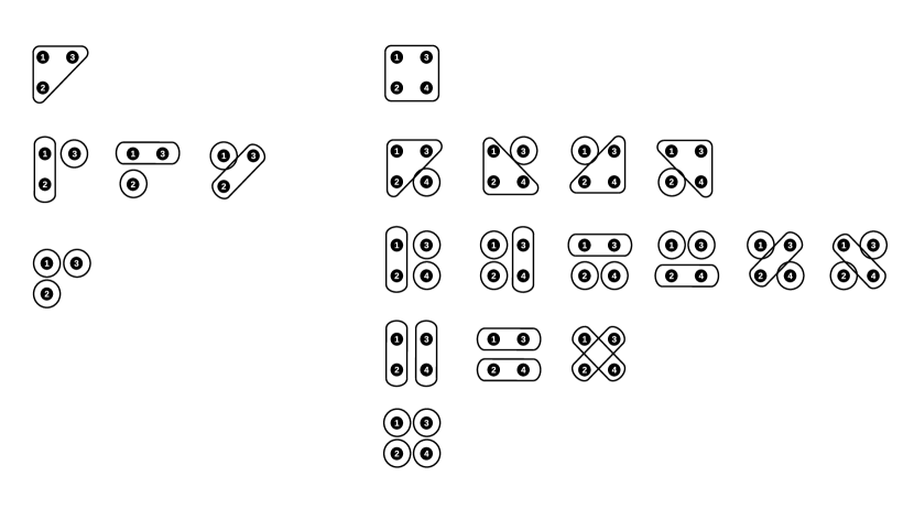
For order we have:
Once again, we break the summation depending on which particle indices are equal. This will correspond to partitioning a set of elements as shown in Figure 1, right. If all indices are equal, corresponding to the first row in the figure, we have a single term
Corresponding to the second row in the figure, we have four terms of the form
Corresponding to the third row, we have two terms of the form
and four terms of the form
Corresponding to the fourth row we have a term of the form
and two terms of the form
Finally, corresponding to the last row we have a single term
Putting all these terms together, we get, in the order presented above,
| (67) | ||||
It is now time to revisit the relations between the moments and the cumulants of distribution. To better illustrate the point, we start with a univariate distribution . Following the notation developed in section 2.1, we have from the relation between the moment generating function and the cumulant generating function of :
Multiplying both sides by and picking out the terms in the exponential expansions which, when multiplied together, give a power of we have
| (68) |
In the summation, each term corresponds to a set of distinct integers and their associated multiplicities such that
and the summation runs over all such sets. The summation can be limited to and , because , and zero multiplicities are not significant. Each term then represents an “integer partition” of the number into positive integer summands.
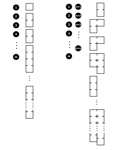
Now consider a partition of a set of distinct objects, as shown in Figure 2, left, that includes blocks of size , blocks of size , , and blocks of size . The number of all possible partitions with those given blocks and their sizes is exactly equal to the coefficient of in (68):
This can be understood by first considering all the permutations of the objects in and among the blocks. The order of placement of the objects within each block does not matter, therefore the division by appears. Finally, the blocks themselves are not ordered, that is, exchanging all the members of a block with all the members of another block of the same size does not create a new partition. Therefore, a division by is necessary.
As a result, a one-to-one correspondence (bijection) exists between each factor that appears in the expansion of and each partition of a set of distinct elements. The mapping is unique in the sense that identical factors of are indistinguishable therefore their permutation yields the same mapping.
There is a parallel situation in the case of a bivariate distribution . Once again, we have from the relation between the moment generating function and the cumulant generating function of :
Multiplying both sides by and picking out the terms in the exponential expansions which, when multiplied together, give a power of we get
| (69) |
Each term in the summation corresponds to a set of distinct ordered pairs with multiplicities subject to the conditions
| (70) |
and
| (71) |
and the summation runs over all such sets. The summation can be limited to (while either or can be zero), and nonzero multiplicities . This will correspond to integer partitioning the ordered pair of positive integers into ordered pairs of positive integers. By ordered, we mean and are different pairs.
Now consider a partition of a set of distinct elements, as shown in Figure 2, right. The set, denoted by , is divided into two complementary subsets and of sizes and respectively. Each block of an arbitrary partition of consists of elements in and elements in , and there are such blocks. Notice that the a block of size is considered to have a different size than a block of size . We claim that the total number of partitions with a given set of blocks and their sizes, that is a given integer partition of , is equal to the coefficient of in (69):
| (72) |
To show this, we argue that only by permuting the members of within and the members of within , all the set partitions of relevant to the given integer partition of are generated. Consider exchanging a member of with a member of . If the exchange happens within the same block, no new partition is created. Therefore it is not counted. If the exchange happens between two distinct blocks, the sizes of the blocks have changed by definition and the resultant set partition of is counted under a different integer partition of . Coefficient (72) then gives the number of all the set partitions relevant to a given number partition, by arguments similar to the univariate case. Each and every partition of is constructed by a partition of together with a permutation of the members of and within their home subsets.
As a result, there is a one-to-one correspondence between the partitions of a set of distinct elements and the products of bivariate cumulants appearing in the expansion of . For each partition there is a product term in the expansion, and for each block of size in the partition there is a in the product term.
On the other hand, we saw that the partitions of a set of distinct elements corresponds uniquely to the terms appearing in the expansion of . Each term in the expansion corresponds to a partition of the set. In each term, groups of equal particle indices, corresponding to the blocks of the partition, break the summation into products of some factors; each factor being of the form:
and in general, for ,
| (73) | ||||
and, for ,
For example, we write the first few in terms of :
and
| (74) |
| (75) |
| (76) | ||||
The functions and are not yet in the form of bivariate moments and cumulants, respectively. They are in fact -variate moments and cumulants of order of the local concentration variables on which they depend. However, consider summation and integration of both sides of the following form; and define
| (77) |
Since each in each term of the expansion of corresponds to a separate block of variables, the integral of their product factorizes into the product of integrals, . Each product term corresponds to an integer partition of the number , and the number of occurrences of such terms is equal to the number of partitions consisting of those block sizes, of a set of distinct objects. All such partitions are constructed by permuting the two groups of and particle indices among themselves, and all such permutations yield the same integration result. Therefore, the relations between and are exactly those between moments and cumulants of a bivariate distribution. Finally, noting that is indeed the th moment of the bivariate distribution (see (50)),
we conclude that are indeed the cumulants of :
| (78) |
We can simply write the first few moments of in terms of its cumulants using (76):
| (79) |
The advantage of cumulant functions, , is that the integrals yield simple analytical forms, and the advantage of functions is that they are simply related to observable intensities. Since the collection of all nonzero cumulants also gives a complete description of the distribution, we can primarily define higher order correlations based on cumulants. To experimentally compute cumulants based on the observed moments of intensity, the inverse relations can be found from (79):
| (80) |
Notice that e.g. can be found by exchanging the subscripts in the relation for , and similarly for and . As a general rule, the coefficients in (80) are obtained from the coefficients in (79) multiplied by where is the total number of blocks in the partition (To see this, compare (68) and (85)).
Conversion to central moments
The relations involving central moments rather than moments are significantly simpler to write and handle. We define
where
We first explain the method suggested by Palmer and Thompson, then explain an easier method of shifting the origin. They write
Comparing with (74) we obtain
Similarly,
For order we have
Then substituting the already calculated and with and respectively and comparing with (75) we obtain
and the procedure can continue to all higher orders.
However, one can see that this procedure is equivalent to shifting the origin such that
for all , also
Therefore, the relations for central moments instead of moments are obtained simply by dropping the terms that contain any (any ) in (65)–(67), the terms that contain any or in (74)–(76), the terms that contain any or in (79), and the terms that contain any or in (80), and removing the primes on any remaining and letters. The latter two sets of relations then become the known relations between the central moments and the cumulants of the bivariate distribution :
and
4.2 Melnykov-Hall approach
This derivation exploits the additive property of cumulants. It was first presented by Melnykov and Hall [9] to derive higher order correlations, following the work of Müller [10] in the context of Fluorescence Cumulant Analysis. We review the derivation in the context of multi-state reacting and diffusing particles.
For a single particle we have (similar to (64) but without summation)
| (81) | ||||
where is given by (60). Substituting this into (50) we obtain, after summation and integration of delta functions, the th moment of the intensity vector for a single particle:
| (82) |
where we have defined:
| (83) |
the single-molecule reaction factor:
and the spatial factor:
| (84) |
The volume of the molecular detection function, , is defined in (58).
Now consider the relation between the cumulant generating function and the moment generating function of a bivariate distribution (see (5)):
where we have used . Through multinomial expansion of the last expression and equating the powers of on the two sides, we obtain:
| (85) |
where the summation is subject to the conditions (70) and (71), corresponding to integer partitioning of the ordered pair into blocks of size and multiplicity , and is the number of blocks in each partition:
This shows that for the intensity vector arising from one particle, we have
where denotes a linear combination of the products of the moments of lower order. Now we use the additive property of cumulants, (8), to write the cumulant of the sum of independent intensity vectors, , arising from independent molecules in the sample volume :
In the thermodynamic limit , this becomes
| (86) |
which, upon substitution from (82), yields
| (87) |
and, using (48),
| (88) |
where we have defined
| (89) |
and
(also defined in (57)) is the expected number of molecules in state in the observation volume.
4.3 Normalized higher order correlations***The content of this section is available in references [1, 2] and is brought here for the sake of continuity.
Given the simpler analytical form of cumulants to study a system of diffusing molecules in solution, we define normalized higher order correlations, with , as
which, in a multi-detector experiment (and/or sub-binning approach) with defined in (46), becomes
| (90) |
and in a single-detector experiment, with , becomes, as obtained by Melnykov and Hall[9],
| (91) |
The two forms follow directly from (45) and (47):
| (92) |
Using (88) in the limit , we obtain the simple analytical form
| (93) |
for the normalized correlation functions, where
is defined in (83),
and is defined in (84).
In practice, one of the parameters can be found from the mean channel count rate, (56):
Without loss of generality, it can be taken to be the first brightness level . Thus a set of and remain to be determined, as well as the reaction relaxation times which result from .
Alternatively, we can define
as the total number of molecules in the probe region regardless of their state. Then we have
where
and
are the concentration (equilibrium constant) and brightness of state relative to state 1. Obviously, and . Thus the number of independent parameters has not changed: and (again, plus the relaxation times). In practice, the rate constants constructing may be more desirable to find. In that case, the system is inversely solved to find the rate constants using the relations that link and relaxation times to the rate constants, and possibly the detailed balance relations.
Here, the usefulness of the factorized form of (93) for obtaining information on multi-state reactions becomes evident. The factors and depend only on the illumination profile and the diffusion constant. Therefore, if the reaction parameters, including rates, relative concentrations, and the relative brightness values are of interest only, then higher order correlations from a “reference” sample with identical diffusional properties can be used to extract the relative reaction function
This eliminates the need to characterize the illumination profile and calibrate the beam shape and diffusion parameters, greatly simplifying the technique and making it more accurate. In practice, the reference sample can consist of non-reacting molecules, or reacting molecules labeled such as to remains in a single brightness state. In this case, we simply have and we get
| (94) |
where
The ratio of the concentration of the sample of interest (“test” sample) to that of the reference sample, , can be obtained either as a fitting parameter in higher-order FCS, or, if possible, through independent techniques such as UV-Vis to reduce the number of higher order correlations required. The values of the absolute parameters , , and are usually of no general interest since they depend on the experimental setup. However, they can be determined using , measured for example by second-order FCS, and the mean detector count, .
5 Variance of correlations
In a multi-detector (and/or sub-binning) approach we have
in a population, and
in a sample.
Using (144), the sampling variance of is related to sampling moments of -statistics:
| (95) |
Unless specified otherwise, the cumulants and -statistics are of random vector (the multi-channel photon count) defined as
The signal-to-noise ratio is defined as
5.1 Order (1,1)
We need to find
By definition
and as shown in (146)
Thus
Now we can add a zero subscript to both sides:
| (97) | ||||
Here we will use the formulae written in “tensor notation” by Kaplan[6] (also listed in [15]). In tensor notation,
and so forth.
As a simple formula in this notation (see (152)),
which means
| (98) |
As another useful formula (see (153)):
meaning
Merging (adding and replacing) the first two rows (i.e. the first two variates are identical) we get
| (99) |
Multivariate cumulants are symmetric functions, thus we can exchange the matrix columns.
In a similar way we have:
which means
| (100) |
Merging the last two rows
| (101) |
We could also obtain this by exchanging the subscripts in (99), however, the intermediate relation will be useful (100) later.
Kaplan’s Equation (3) reads:
In the summation, and indicate whichever of the first two subscripts that are nonzero. and indicate whichever of the last two subscripts that are nonzero. All other subscripts in each must be zero. , , and must be non-identical. The summation superscript indicates that there are two distinct terms of such kind. Thus we have:
| (102) |
Merging row with row , and row with row , we get
| (103) |
The right hand side is in terms of cumulants of (the multi-channel photon count) which have not been calculated, while the cumulants of (the underlying integrated intensity) have been calculated in (88):
| (104) |
To simplify matters, we only consider the shot-noise-dominant limit in which and
and to further simplify, we only consider a single species, thus:
Therefore (104) becomes
| (105) |
where is the average number of photons per bin. Here, we assume the shot-noise-dominant regime, that is
On the other hand, factorial cumulants of are equal to cumulants of , by (44):
| (106) |
where can have elements greater than , and is constructed by merging the elements of that are at identical lag times (i.e. identical ). Therefore, to calculate the cumulants of , as in (103), we express them in terms of factorial cumulants of . The conversion relations are formally similar to those between moments and factorial moments, and are given in (36). Using those, and (103) in the limit , we write
| then using (105) and (106) | ||||
having used .
Following a similar approach, one can show that the order difference between the denominator and the numerator does not exceed in any other term in (96) when written in the form of factorial cumulants, thus they can all be neglected, and the SNR becomes
| (107) |
5.2 Order (2,1)
For the sampling variance of
we need to calculate
Extending the univariate case by adding a neutral subscript, as in (97),
| (108) |
and extending the bivariate case (103)
| (109) |
where we have kept the lowest-order term(s) in conversion to factorial cumulants for later use.
Using the rule of Appendix C again we have:
meaning
Merging the last two rows:
| (113) | ||||
| (114) |
And, is already calculated in (100).
Kaplan’s Equation (4) reads:
which is a shorthand notation for
where the matrix in front of the summation lists the summed terms. To obtain , we merge the rows according to a “subscript identicality pattern” of the form , which means the first and the third rows (subscripts) are merged together and used as the new first row, the second and the fourth rows are merged together to form the new second row, and the fifth row forms the new third row as is. This yields
| (124) | ||||
| (125) |
Upon conversion to factorial cumulants, a with a subscript of, say, breaks down to plus , and we care about the lowest-order terms in only.
Using Kaplan’s Equation (7):
which becomes
The procedure can be computerized to produce all terms of a particular form. The program is included in Supporting Information.
Using the identicality pattern , then converting to factorial cumulants and keeping the lowest-order terms:
| (135) | ||||
| (139) | ||||
| (140) |
We are now ready to evaluate the following terms:
From (108):
From (109):
From (140):
From (114):
From (125):
From (100):
Therefore the largest oder in is the term which dominates the relative uncertainty. This was expected, as the -statistics of higher order have larger relative uncertainties in the shot-noise-dominated regime. Thus, using (140)
Finally,
| (141) |
Comparing with the single-detector result reported by Melnykov and Hall [9],
we see that the presence of two independent channels contributes positively by a factor of . This is intuitive by considering the fact that if are independent random variables with identical distribution, we have
However, it should also be noted that splitting the beam among detectors is equivalent to reducing the brightness by a factor of . The SNR has a power of for each higher order. Also, sub-binning reduces the effective bin size, . Combining multiple ways to selection sub-bins partially makes up for the loss. Therefore, comparing the overall single-detector and multi-detector SNR requires more detailed analysis for each order. An optimally large bin size usually ensures sufficient SNR in each method.
Before we finish this section, we point out that the single-detector can be obtained from
where the random variables are . The denominator is the same as in multi-detector case. To calculate the numerator, we use
which yields
We can obtain by merging the first two subscripts in the result for (Equation (139)). Similarly, is obtained by merging the last two subscripts in (Equation (124)) and swapping the subscripts. The result then has to be converted back to factorial cumulants and the lowest-order terms kept to obtain .
5.3 Order (2,2)
Now for the sampling variance of
we need to calculate
Simply by rewriting (109) with a neutral 4th subscript, we have
and is obtained by swapping the first two and last two indices.
Also, is already given in (102), which has the same factorial form.
We invoke Kaplan’s Equation (5)
which yields
With subscript identicality pattern we get
Similarly, is of order .
To calculate we use Kaplan’s Equation (10), (with a correction in the number of terms of ):
This directly yields
With the identicality pattern ,
Converting to factorial cumulants and keeping the lowest-order terms
Assuming and using (105),
| (142) | ||||
Now we can verify,
Therefore has the lowest order in as expected.
The SNR results, (107), (141), and (143), are consistent with
reported by Melnykov and Hall (they have not reported specifically, and we have not calculated it yet either; it is, as one might expect, a tedious task). “In the high-concentration limit, a fluorescence signal becomes Gaussian and therefore correlations other than tend to 0. When SNR is independent of the number of molecules in the high concentration limit and is proportional to N in the low concentration limit.” In our current report and experiments, the highest order studied is which has our limiting uncertainty. Therefore, assuming a Gaussian illumination profile which yields
we estimate the optimal value of that maximizes (143) to be , with half maxima at , corresponding to correlation amplitudes of
or ( is a more common definition of the number of molecules in the probe region in conventional FCS.) The numbers in parentheses indicate the values at half maxima of .
To examine the validity of the assumption at large lag times, consider the lag time and , with and channel count rate . We then have then . But this is about the limit in our experiments. As long as is not true, and , the truncated formulas above give the right order of magnitude.
In our program implementation, we estimate using , with (ideally, ) being the mean photon count per bin, and calculated using the inverse of :
This result assumes not reaction. For reactions, further analysis is needed.
Appendix A Variance and covariance of a function
The following derivation is described in [15]. Suppose for we have
(usually ) then as . For example, can be statistics.
Consider
Through Taylor expansion we have
Since we have
Now
| assuming not all | ||||
| (144) | ||||
Permutation is allowed in the second summation.
In particular, if is a linear function of random variables: then
Similarly, one can show
Appendix B Some sampling moments
There are three types of moments:
-
•
Population moments (moments of the population), such as , , etc.
-
•
Sample moments (moments of the sample), such as , , etc.
-
•
Sampling moments (moments of the sampling distribution), such as , , , , etc.
Similarly we have population cumulants, sample cumulants, and sampling cumulants.
Specifically, the th moment is , the th moment statistic is
and the th central moment statistic (moment about the sample mean) is
| (145) |
Here, we aim to find to the first few sampling moments. The material is adopted from [15].
The expectation of is
The sampling variance of is
| The second summation has terms with and independent | ||||
| (146) | ||||
which is an exact result.
The expectation of is
Since and are independent, and
we get
Thus, asymptotically,
To calculate the sampling variance of , we shall generalize this approach for higher moments. Recall e.g.
has terms. To simplify the notation, we define the following variants of symmetric functions. A symmetric function remains unchanged if we permute the s.
-
•
Augmented symmetric functions: (all subscripts different)
(147) E.g.
-
•
Monomial symmetric functions:
-
•
Unitary functions (no two indices equal):
-
•
One-part functions or power sums:
From (147)
| (148) |
where and is the “weight” of the symmetric function.
For example, the sample variance (145) for becomes
We have,
(or from table). Hence,
| (149) |
Now using (148)
| (150) |
For a shortcut to calculate such expectation values, notice that statistic is independent of the origin. Therefore, we can take the population mean to be zero: . Then ignore any containing a unit and (149) immediately gives (150).
Similarly,
From table or directly
since
and
because
Ignoring ’s containing a unit:
| and using (148) | ||||
Using this and (150) we get
| (151) | ||||
where indicates asymptotic equality at large .
Also, if in (151) we put and and
Appendix C A tensor notation rule
In Kaplan’s formulae in tensor notation for cumulants of -statistics[6], to insert a single subscript, we affix the subscript in every possible position and divide by . For example, given
we can construct
Other examples:
| (152) |
| (153) |
Appendix D Two-state transition factors
Consider a fluorescent particle alternating between two states:
where “state 1” is usually the brighter (unfolded) state, “state 2” is usually the darker (folded) state, and and are the forward and backward (reverse) rates respectively. Denote the probability that the particle is found in state at time time with , and similarly for state . The following equations describe the reaction:
The solutions are
| (154) | ||||
where and are the initial probabilities at time . We have defined
with being the number of molecules in state in the ensemble, and
as the overall reaction time constant. Also, defining
as the probability of finding the particle in state independent of initial conditions, we have
The transition factor , denoting the probability that the particle is found in state at time given it was in state at time , can be found by setting the initial probabilities in (154) equal to or :
References
- [1] Farshad Abdollah-Nia, Martin P. Gelfand, and Alan Van Orden. Artifact-free and detection-profile-independent higher-order fluorescence correlation spectroscopy for microsecond-resolved kinetics. 1. multidetector and sub-binning approach. The Journal of Physical Chemistry B, 121(11):2373–2387, 2017. PMID: 28230994.
- [2] Farshad Abdollah-Nia, Martin P. Gelfand, and Alan Van Orden. Artifact-free and detection-profile-independent higher-order fluorescence correlation spectroscopy for microsecond-resolved kinetics. 2. mixtures and reactions. The Journal of Physical Chemistry B, 121(11):2388–2399, 2017. PMID: 28182427.
- [3] N Balakrishnan, Norman L Johnson, and Samuel Kotz. A note on relationships between moments, central moments and cumulants from multivariate distributions. Statistics & probability letters, 39(1):49–54, 1998.
- [4] Elliot L Elson and Douglas Magde. Fluorescence correlation spectroscopy. i. conceptual basis and theory. Biopolymers, 13(1):1–27, 1974.
- [5] Lindsey N Hillesheim and Joachim D Müller. The dual-color photon counting histogram with non-ideal photodetectors. Biophysical Journal, 89(5):3491–3507, 2005.
- [6] E. L. Kaplan. Tensor notation and the sampling cumulants of -statistics. Biometrika, 39(3/4):319–323, 1952.
- [7] Oleg Krichevsky and Grégoire Bonnet. Fluorescence correlation spectroscopy: the technique and its applications. Reports on Progress in Physics, 65(2):251, 2002.
- [8] L Mandel. Fluctuations of photon beams and their correlations. Proceedings of the Physical Society, 72(6):1037, 1958.
- [9] Artem V Melnykov and Kathleen B Hall. Revival of high-order fluorescence correlation analysis: generalized theory and biochemical applications. The Journal of Physical Chemistry B, 113(47):15629–15638, 2009.
- [10] Joachim D Müller. Cumulant analysis in fluorescence fluctuation spectroscopy. Biophysical Journal, 86(6):3981–3992, 2004.
- [11] A.G. Palmer and N.L. Thompson. Molecular aggregation characterized by high order autocorrelation in fluorescence correlation spectroscopy. Biophysical Journal, 52(2):257 – 270, 1987.
- [12] Arthur G Palmer and Nancy L Thompson. High-order fluorescence fluctuation analysis of model protein clusters. Proceedings of the National Academy of Sciences, 86(16):6148–6152, 1989.
- [13] Arthur G Palmer III and Nancy L Thompson. Intensity dependence of high-order autocorrelation functions in fluorescence correlation spectroscopy. Review of Scientific Instruments, 60(4):624–633, 1989.
- [14] Perry G. Schiro, Christopher L. Kuyper, and Daniel T. Chiu. Continuous-flow single-molecule ce with high detection efficiency. ELECTROPHORESIS, 28(14):2430–2438, 7 2007.
- [15] Alan Stuart and Keith Ord. Kendall’s advanced theory of statistics, volume 1. Arnold, a member of the Hoddder Headline Group, 4th edition, 1994.
- [16] Alan Van Orden, Keir Fogarty, and Jaemyeong Jung. Fluorescence fluctuation spectroscopy: a coming of age story. Applied spectroscopy, 58(5):122A–137A, 2004.
- [17] Bin Wu, Yan Chen, and Joachim D Müller. Dual-color time-integrated fluorescence cumulant analysis. Biophysical Journal, 91(7):2687–2698, 2006.
- [18] Bin Wu and Joachim D Müller. Time-integrated fluorescence cumulant analysis in fluorescence fluctuation spectroscopy. Biophysical Journal, 89(4):2721–2735, 2005.
- [19] Zhenqin Wu, Huimin Bi, Sichen Pan, Lingyi Meng, and Xin Sheng Zhao. Determination of equilibrium constant and relative brightness in fluorescence correlation spectroscopy by considering third-order correlations. The Journal of Physical Chemistry B, 120(45):11674–11682, 2016. PMID: 27775360.