Utility Change Point Detection in Online Social Media: A Revealed Preference Framework

Abstract

This paper deals with change detection of utility maximization behaviour in online social media. Such changes occur due to the effect of marketing, advertising, or changes in ground truth. First, we use the revealed preference framework to detect the unknown time point (change point) at which the utility function changed. We derive necessary and sufficient conditions for detecting the change point. Second, in the presence of noisy measurements, we propose a method to detect the change point and construct a decision test. Also, an optimization criteria is provided to recover the linear perturbation coefficients. Finally, to reduce the computational cost, a dimensionality reduction algorithm using Johnson-Lindenstrauss transform is presented. The results developed are illustrated on two real datasets: Yahoo! Tech Buzz dataset and Youstatanalyzer dataset. By using the results developed in the paper, several useful insights can be gleaned from these data sets. First, the changes in ground truth affecting the utility of the agent can be detected by utility maximization behaviour in online search. Second, the recovered utility functions satisfy the single crossing property indicating strategic substitute behaviour in online search. Third, due to the large number of videos in YouTube, the utility maximization behaviour was verified through the dimensionality reduction algorithm. Finally, using the utility function recovered in the lower dimension, we devise an algorithm to predict total traffic in YouTube.

I Introduction

The interaction of humans on social media platforms mimic their interactions in the real world [1]. Hence, as in the real world, “utility maximization” underpins human interaction on social media platforms. Utility maximization is the fundamental problem humans face, wherein humans maximize utility given their limited resources of money or attention. Detection of utility maximization behaviour is therefore useful in online social media. However, a key difference for agents in online social media is the absence of economic incentives. For example, the majority of content in Facebook, YouTube and Twitter are user-generated with limited or no economic incentives. Hence, as explained in [2], incentives such as “fun” and “fame” are some of the major attributes of the utility function of online social behaviour. It is therefore difficult to analytically characterize the utility function and hence any detection of utility maximization behaviour in online social media needs to be necessarily nonparametric in nature. Another key difference is that the utility function in online social media is “content-aware”, i.e. the quality of content affects the utility function. Due to the content-aware nature of the utility function and the availability of large amount of user generated content, data from online social media is high-dimensional. For example, utility maximization in YouTube depends on all the user generated video content available at any point of time.

The problem of nonparametric detection of utility maximizing behaviour is the central theme in the area of revealed preferences in microeconomics. This is fundamentally different to the theme used widely in the signal processing literature, where one postulates an objective function (typically convex) and then develops optimization algorithms. In contrast, the revealed preference framework, considered in this paper, is data centric: Given a dataset, $\mathcal{D}$, consisting of probe, $p_{t}\in\mathbb{R}_{+}^{m}$, and response, $x_{t}\in{\rm IR}_{+}^{m}$, of an agent for $T$ time instants:

$$\mathcal{D}=\left\{(p_{t},x_{t}),t=1,2,\dots,T\right\}.$$ (1)

Revealed preference aims to answer the following question: Is the dataset $\mathcal{D}$ in (1) consistent with utility-maximization behaviour of an agent? A utility-maximization behaviour (or utility maximizer) is defined as follows:

Definition I.1.

An agent is a utility maximizer if, at each time $t$, for input probe $p_{t}$, the output response, $x_{t}$, satisfies

$$x_{t}=x(p_{t})\in\underset{\left\{p_{t}^{\prime}x\leq I_{t}\right\}}{\operatorname{argmax}u(x)}.$$ (2)

Here, $u(x)$ denotes a locally non-satiated utility function. Also, $I_{t}\in\mathbb{R}_{+}$, is the budget of the agent. The linear constraint, $p_{t}^{\prime}x\leq I_{t}$ imposes a budget constraint on the agent, where $p_{t}^{\prime}x$ denotes the inner product between $p_{t}$ and $x$.

Major contributions to the area of revealed preferences are due to Samuelson [3], Afriat [4], Varian [5], and Diewert [6] in the microeconomics literature. Afriat [4] devised a nonparametric test (called Afriat’s theorem), which provides necessary and sufficient conditions to detect utility maximizing behaviour for a dataset. For an agent satisfying utility maximization, Afriat’s theorem [4] (stated below in Theorem II.1) provides a method to reconstruct a utility function consistent with the data. The utility function, so obtained, can be used to predict future response of the agent. Varian [7] provides a comprehensive survey of revealed preference literature.

Despite being originally developed in economics, there has been some recent work on application of revealed preference to social networks and signal processing. In the signal processing literature, revealed preference framework was used for detection of malicious nodes in a social network in [8, 9] and in demand estimation in smart grids in [10]. [11] analyzes social behaviour and friendship formation using revealed preference among high school friends. In online social networks, [12] uses revealed preference to obtain information about products from bidding behaviour in eBay or similar bidding networks.

I-A The Problem: Utility Change Point Detection in Online Social Media.

In this paper, we consider an extension of the classical revealed preference framework of [4] to agents with “dynamic utility function”. The utility function jump changes at an unknown time instant by a linear perturbation. Given the dataset of probe and responses of an agent, the objective is to develop a nonparametric test to detect the change point and the utility functions before and after the change, which is henceforth referred to as the change point detection problem.

Such change point detection problems arise in online search in social media. The online search is currently the most popular method for information retrieval [13]. The online search process can be seen as an example of an agent maximizing the information utility, i.e. the amount of information consumed by an online agent given the limited resource on time and attention. There has been a gamut of research which links internet search behaviour to ground truths such as symptoms of illness, political election, or major sporting events [14, 15, 16, 17, 18, 19]. Detection of utility change in online search, therefore, is helpful to identify changes in ground truth and useful, for example, for early containment of diseases [15] or predicting changes in political opinion [20, 21]. Also, the intrinsic nature of the online search utility function motivates such a study under a revealed preference setting.

The problem of studying agents with dynamic utility functions, with a linear perturbation change in the utility function is motivated by several reasons. First, it provides sufficient selectivity such that the non-parametric test is not trivially satisfied by all datasets but still provides enough degrees of freedom. Second, the linear perturbation can be interpreted as the change in the marginal rate of utility relative to a “base” utility function. In online social media, the linear perturbation coefficients measure the impact of marketing or the measure of severity of the change in ground truth on the utility of the agent. This is similar to the linear perturbation models used to model taste changes [22, 23, 24, 25] in microeconomics. Finally, in social networks, linear change in the utility is usually used to model the change in utility of an agent based on the interaction with the agent’s neighbours [26]. Compared to the taste change model, our model is unique in that we allow the linear perturbation to be introduced at an unknown time. To the best of our knowledge, this is the first time in the literature that change point detection problem has been studied in the revealed preference setting.

A related important practical issue that we also consider in this paper is the high dimensionality of data arising in online social media. As an example of high dimensional data arising in online social media, we investigate the detection of the utility maximization process inherent in one of the most common social media interactions: video sharing via YouTube. Detecting utility maximization behaviour with such high dimensional (big) data is computationally demanding.

The organization of the paper is as follows: In Sec. II, we derive necessary and sufficient conditions for change point detection, for dynamic utility maximizing agents under the revealed preference framework. In Sec. III, we study the change point detection problem in the presence of noise. Section IV address the problem of high dimensional data arising in the context of revealed preference. Section V presents numerical results. First, we compare the proposed approach with the popular CUSUM test and corresponding ROC curves are presented. Second, we illustrate the result developed on two real world datasets: Yahoo! Tech Buzz dataset and Youstatanalyzer dataset.

II Utility Change Point Detection (Deterministic case)

In this section, we consider agents with a dynamic utility function. For completeness, we start with Afriat’s theorem, in the classical static setting. Afriat’s Theoremis one of the big results in revealed preferences in micro-economics theory.

Theorem II.1 (Afriat’s Theorem [4]).

Given the dataset $\mathcal{D}$ in (1), the following statements are equivalent:

1. The agent is a utility maximizer and there exists a monotonically increasing and concaveutility function that satisfies (2).

2. For $u_{t}$ and $\lambda_{t}>0$ the following set of inequalities has a feasible solution:

   $$u_{s}-u_{t}-\lambda_{t}p_{t}^{\prime}(x_{s}-x_{t})\leq 0\;\forall t,s\in\{1,2,\dots,T\}.\$$ (3)

3. A monotonic and concave utility function that satisfies (2) is given by:

   $$u(x)=\underset{t\in\{1,2,\dots,T\}}{\operatorname{min}}\{u_{t}+\lambda_{t}p_{t}^{\prime}(x-x_{t})\}$$ (4)

4. The dataset $\mathcal{D}$ satisfies the Generalized Axiom of Revealed Preference (GARP), namely for any $t\leq T$, $p_{t}^{\prime}x_{t}\geq p_{t}^{\prime}x_{t+1}\quad\forall t\leq k-1\implies p_{k}^{\prime}x_{k}\leq p_{k}^{\prime}x_{1}.\qed$

The remarkable property of Afriat’s Theorem is that it gives necessary and sufficient conditions for the dataset to satisfy utility maximization (2). The feasibility of the set of inequalities can be checked using a linear programming solver or by using Warshall’s algorithm with $O(T^{3})$ computations [7] [5]. A utility function consistent with the data can be constructed using (4). The recovered utility is not unique since any monotonic transformation of (4) also satisfy Afriat’s Theorem.

II-A System Model

In this paper, we consider an agent that maximizes a utility function that jump changes by a linear perturbation at a time that is unknown to the observer. The aim is to estimate the utility before and after the change, and the change point. Consider an agent that selects a response $x$ at time $t$ to maximize the utility function given by:

$$u(x,\alpha;t)=v(x)+\alpha^{\prime}x\mathds{1}\{t\geq\tau\},$$ (5)

subject to the following budget constraint $p_{t}^{\prime}x\leq I_{t}$. Here, $\mathds{1}\{\cdot\}$ denotes the indicator function. The utility function, $u(x,\alpha;t)$ consists of two components: a base utility function, $v(x)$, and a linear perturbation, $\alpha^{\prime}x$, which occurs at an unknown time $\tau$. The base utility function, $v(x)$ is assumed to be monotonic and concave. We will restrict the components of the vector $\alpha$ to be (strictly) greater than 0, so that the utility function, $u$, conditioned on $\alpha$ is monotonic and concave. The objective is to derive necessary and sufficient conditions to detect the time, $\tau$ at which linear perturbation is introduced to the base utility function. Theorem II.2 summarizes the necessary and sufficient conditions to detect the change in utility function according to the model in (5) and the proof is in Appendix A-A.

Theorem II.2.

The dataset $\mathcal{D}$ in (1) is consistent with the model in (5) if we can find set of scalars $\{v_{t}\}_{t=1,\dots,T}$, $\{\lambda_{t}>0\}_{t=1,\dots,T}$, $\{\alpha_{k}\}_{k=1,\dots,m}$, such that there exists a feasible solution to the following inequalities:

$$v_{t}+\lambda_{t}p_{t}^{\prime}(x_{s}-x_{t}) \geq v_{s} (t<\tau)$$ (6)

$$v_{t}+\lambda_{t}p_{t}^{\prime}(x_{s}-x_{t})-\alpha^{\prime}(x_{s}-x_{t}) \geq v_{s} (t\geq\tau)$$ (7)

$$\alpha_{i} \leq\lambda_{t}p_{t}^{i} (\forall i,t\geq\tau),$$ (8)

where $p_{t}^{i}$ is the $i$^th component of the probe $p_{t}$.

The inequalities in eqs. 6, 7 and 8 closely resemble the Afriat inequalities (3). The time instant $\tau$ at which the inequalities are satisfied is the time at which the linear perturbation is introduced.

II-B Recovery of minimum perturbation of $\alpha$ and the base utility function

Computing the linear perturbation coefficients in (5) gives an indication of the severity of the ground truth or the effect of marketing and advertising in social media. The solution to the following convex optimization provides the minimum value of the perturbation coefficients:

min $$\lVert\alpha\rVert_{2}^{2}$$ (9)

s.t.

$$\geq\scalebox{0.95}{$v_{s}\phantom{p_{t}^{i}}\phantom{\forall i,}(t\geq\tau)$}$$ (11)

$$\leq\scalebox{0.95}{$\lambda_{t}p_{t}^{i}(\forall i,t\geq\tau)$}$$ (12)

(13)

where, $\beta$ and $\delta$ are arbitrary constants.

The equations (10) to (12) correspond to the revealed preference inequalities eqs. 6, 7 and 8. The normalization conditions eq. 13 are required because of the ordinalityof the utility function. This is because for any set of feasible values of $\{v_{t}\}_{t=1,\dots,T}$, $\{\lambda_{t}\}_{t=1,\dots,T}$, $\{\alpha_{k}\}_{k=1,\dots,m}$ satisfying the constraints in Theorem II.2 the following relation also holds

$$\beta(v_{s}+\delta)-\beta(v_{t}+\delta)-\beta\lambda_{t}{p}_{t}^{\prime}(x_{s}-x_{t})+\beta\alpha^{\prime}(x_{s}-x_{t})\leq 0.$$

Recall that the base utility function $v(x)$, is the utility function before the linear change.

Corollary II.1.

The recovered base utility function is

$$\hat{v}(x)=\underset{t}{\min}\{v_{t}+\lambda_{t}\tilde{p}_{t}^{\prime}(x-x_{t})\},$$ (14)

where

$$\tilde{p}_{t}^{i}=\begin{cases}p_{t}^{i}&t<\tau,\\ p_{t}^{i}-\alpha_{i}/\lambda_{t}&t\geq\tau.\end{cases}$$ (15)

In eqs. 14 and 15 $\{v_{t}\}$, $\{\lambda_{t}\}$, $\{\alpha_{k}\}$ are the solution of eqs. 9, 10, 11, 12 and 13.

II-C Comparison with classical change detection algorithms

Method	Data model	Change model	Reference
CUSUM	$x_{t}\overset{i.i.d}{\sim}p_{\theta}$	$\theta=\begin{cases}\theta_{0}&t<\tau\\ \theta_{1}&t\geq\tau\end{cases}$	[27]
Semi-supervised/Supervised	$\mathcal{D}=\left\{\left((p_{1},I_{1}),U(p_{1},I_{1})\right),\dots,\left((p_{T},I_{T}),U(p_{T},I_{T})\right)\right\}$	Not Applicable	[28, 29, 30]
Learning	$\left(p_{i},I_{i}\right)\sim P$, $U(p_{i},x_{i})$: Optimal response for utility $U$		[31]
Revealed Preference	$x_{t}=\underset{p_{t}^{\prime}x_{t}\leq I_{t}}{\operatorname{argmax}\;}u(x_{t})$	$u(x)=\begin{cases}v(x)&t<\tau\\ v(x)+\alpha^{\prime}x&t\geq\tau\end{cases}$	This paper

TABLE I: Comparison of Revealed Preference with classical change detection algorithm.

Table I compares the revealed preference framework of our paper with classical change detection algorithms. The key difference is that the revealed preference framework considers a system with maximization of a utility function subject to linear constraints (the budget constraint). In comparison, a classical CUSUM type change detection algorithm requires knowledge of a parametrized utility function (see Sec. V-A for a numerical example when $v(x)$ is a Cobb-Douglasutility function). The revealed preference framework for change detection makes no such assumptions. The revealed preference problem is related to the supervised learning literature when the parametric class of functions for empirical risk minimization (ERM) is limited to concave and monotone functions [28, 29, 30]. The change detection problem can be thought of as a multi-class learning problem with the first class being the utility function before the change and the second class being the utility function after the change. However, this paper provides an algorithmic approach to detect change points by deriving necessary and sufficient conditions.

III Utility change point detection in noise

Sec. II dealt with utility change point detection in the deterministic case. In this section, we consider the change point detection problem when the response of the agent is measured in noise.

III-A Classical revealed preference in a noisy setting

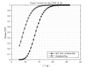
Figure 1: Comparison of analytical expression with M.C. simulation: Upper bound on the CDF of $M$, as defined in (21). (Lower bound on the false alarm probability.)

Afriat’s theorem (Theorem II.1) assumes perfect observation of the probe and response. However, when the response of the agents are measured in noise, the failure of Afriat test could be either due to measurement noise or absence of utility maximization. Below, we assume the additive noise model for measurement errors given by:

$$y_{t}=x_{t}+w_{t},$$ (16)

where $y_{t}$ is the noisy measurement of response $x_{t}$ and $w_{t}\in\mathbb{R}^{m}$ is the independent and identically distributed (i.i.d) standard Gaussian noise.

Given the noisy dataset

$$\mathcal{D}_{\text{obs}}=\left\{\left(p_{t},y_{t}\right):t\in\left\{1,\dots,T\right\}\right\},$$ (17)

[8] proposes the following statistical test for testing utility maximization (2) in a dataset due to measurement errors. Let $H_{0}$ denote the null hypothesis that the dataset $\mathcal{D}_{\text{obs}}$ in (17) satisfies utility maximization. Similarly, let $H_{1}$ denote the alternative hypothesis that the dataset does not satisfy utility maximization. There are two possible sources of error:

Type-I errors:   Reject $$H_{0} H_{0}$$ when is valid.

Type-II errors:   Accept $$H_{0} H_{0}$$ when is invalid. (18)

The following statistical test can be used to detect if an agent is seeking to maximize a utility function.

$$\boxed{\phantom{\text{\hskip 0.56905pt}}\int\limits_{\Phi^{*}(\bf y)}^{+\infty}f_{M}(\psi)\mathrm{d}\psi\overset{H_{0}}{\underset{H_{1}}{\gtrless}}\gamma}.$$ (19)

In the statistical test, (19):
(i) $\gamma$ is the “significance level” of the statistical test.
(ii) The “test statistic” $\Phi^{*}(\bf y)$, with ${\bf y}=\left[y_{1},y_{2},\dots,y_{T}\right]$ is the solution of the following constrained optimization problem :

$$\begin{array}[]{rl}\min&\Phi\\ \mbox{s.t.}&u_{s}-u_{t}-\lambda_{t}p_{t}^{\prime}(y_{s}-y_{t})-\lambda_{t}\Phi\leq 0\\ &\lambda_{t}>0\quad\Phi\geq 0\quad\text{for}\quad t,s\in\{1,2,\dots,T\}.\end{array}$$ (20)

(iii) $f_{M}$ is the pdf of the random variable $M$ where

$$M\triangleq\underset{\underset{t\neq s}{t,s}}{\max}\left[p_{t}^{\prime}(w_{t}-w_{s})\right].$$ (21)

The probability of false alarm or Type-I error, the probability of rejecting $H_{0}$, when true, is given by $\mathbb{P}\left\{M\geq\Phi^{*}(\bf y)\right\}$.

Below, we derive an analytical expression for the lower bound for the false alarm probability of the statistical test in (19). The motivation comes from the following fact: Given the significance level of the statistical test in (19), a Monte Carlo (M.C.) simulation is required to compute the threshold. However, from an analytical expression for the lower bound on false alarm probability, we can obtain an upper bound of the test statistic, denoted by $\overline{\Phi^{*}(\bf y)}$. Hence, for any dataset $\mathcal{D}_{\text{obs}}$ in (17), if the solution to the optimization problem (20) is such that $\Phi>\overline{\Phi^{*}(\bf y)}$, then the dataset does not satisfy utility maximization, for the desired false alarm probability.

Theorem 22 provides the lower bound on the false alarm probability and the proof is provided in Appendix A-C.

Theorem III.1.

If the noise components have a standard Gaussian distribution, then the probability of false alarm is lower bounded by

$$1-\underset{t}{\prod}\left\{1-\sqrt{\frac{2}{\pi}}\frac{\sqrt{2{\lVert p_{t}\rVert}^{2}}\exp{(-{\Phi^{*}({\bf y})}^{2}/4{\lVert p_{t}\rVert}^{2})}}{{\Phi^{*}({\bf y})}+\sqrt{{\Phi^{*}({\bf y})}^{2}+8{\lVert p_{t}\rVert}^{2}}}\right\}.$$ (22)

The key idea is to bound $M$ in (21) by the highest order statistic of a carefully chosen set of random variables which are negatively dependent. Refer to Appendix A-B for the definition of negative dependence.

Figure 1 shows the comparison of the upper bound of the cdf (and correspondingly the lower bound on the false alarm probability) and the M.C. simulation of actual density of $M$. As can be seen from Fig 1 that the upper bound of the cdf (lower bound on false alarm probability) is tight at all regimes. The upper bound of the test statistic, $\overline{\Phi^{*}(\bf y)}$, can be obtained by setting the analytical expression in (22) to be equal to the desired false alarm probability.

III-B Dynamic Revealed Preference in a noisy setting

In this section, we consider the case of dynamic utility maximizing agents, satisfying the model in (5), in the presence of noise. In Sec. III-B1, we propose a procedure to detect the unknown change point time in presence of noise. In Sec. III-B2, similar to Sec. III-A, we formulate a hypothesis test to check whether the dataset satisfy the model in (5). As in Sec. III-A, we bound the false alarm probability and obtain a criteria for recovering the linear perturbation coefficient, corresponding to minimum false alarm probability. Once the unknown change point time and the linear perturbation coefficients have been recovered, the base utility function can be recovered similar to that in Sec. II-B.

III-B1 Estimation of unknown change point

In the presence of noise, the inequalities in (6) to (8) may not be satisfied for any value of $\tau$. Hence, we consider the following linear programming problem, to find the minimum error or “adjustment” such that the inequalities in (6) to (8) are satisfied.

$${\Phi_{\tau}}= \text{ min }\Phi$$ (23)

s.t.

$$\leq\scalebox{0.95}{$0\quad\phantom{\forall i,}(t\geq\tau)$}$$

$$\leq\scalebox{0.95}{$0\quad(\forall i,t\geq\tau)$}$$

$$\hskip 60.00009pt\Phi\geq 0,\quad\lambda_{t}>0$$

The solution of the linear program (23) depends on the choice of the change point variable $\tau$. When the data is measured without noise, the equations are satisfied with zero error at the correct change point. The estimated change point, $\hat{\tau}$, corresponds to time point with minimum adjustment.

$$\hat{\tau}=\underset{1\leq\tau\leq T}{\operatorname{argmin}\;}\Phi_{\tau}$$ (24)

The intuition for (24) is if ${\tau}$ is the true change point, then the perturbation $\Phi$ needs to compensate only for the noise.

III-B2 Recovering the linear perturbation coefficients for minimum false alarm probability

As in (18), define the null hypothesis $H_{0}$, that the dataset satisfies utility maximization under the model in (5), and the alternative hypothesis $H_{1}$ that the dataset does not satisfy utility maximization under the model in (5). Type-I errors and Type-II errors are defined, similarly, as in Sec. III-A.

Consider the following hypothesis test:

$$\boxed{\phantom{\text{\hskip 0.56905pt}}\int\limits_{\Phi^{*}(\bf y)}^{+\infty}f_{M}(\psi)\mathrm{d}\psi\overset{H_{0}}{\underset{H_{1}}{\gtrless}}\gamma}.$$ (25)

In (25):

1. $\gamma$ is the significance level of the test.

2. The test statistic “$\Phi^{*}({\bf y})$”, is the solution of the following constrained optimization problem with $\tau=\hat{\tau}\text{ (from Sec.\@~{}\ref{subsubsec:detect:changepoint:noise})}$.

   min $$\Phi$$ (26)

   s.t.

   $$\leq\scalebox{0.95}{$0\;(\forall i,t\geq\tau)$}$$

   $$\hskip 60.00009pt\Phi\geq 0,\quad\lambda_{t}>0$$

   The optimization problem above (26) is similar to the optimization problem (23) but is introduced for simplicity of analysis of the error probability in the subsequent sections.

3. $f_{M}$ is the pdf of the random variable, $M$, where

   $$M\triangleq M_{1}+M_{2},$$ (27)

   where $M_{1}$ and $M_{2}$ are defined as:

   $$M_{1} \triangleq\underset{\underset{s\neq t}{s,t}}{\max}\left[p_{t}^{\prime}(w_{t}-w_{s})\right],$$ (28)

   $$M_{2} \triangleq\underset{\underset{s\neq t,t\geq\tau}{s,t}}{\max}\left[\alpha^{\prime}{(w_{t}-w_{s})}/\lambda_{t}\right],$$ (29)

where $\alpha$ and $\lambda$ are the solution of (26). The set of inequalities in (26) can be re-written using (16) as:

$$(v_{s}-v_{t})/\lambda_{t}-{p}_{t}^{\prime}(x_{s}-x_{t})\leq p_{t}^{\prime}{\left(w_{t}-w_{s}\right)} \quad(t<\tau),$$

$$(v_{s}-v_{t})/\lambda_{t}-{p}_{t}^{\prime}(x_{s}-x_{t})+\alpha^{\prime}(x_{s}-x_{t})/\lambda_{t}\hfil\hfil$$

$$\quad\leq p_{t}^{\prime}{\left(w_{t}-w_{s}\right)}-\alpha^{\prime}{\left(w_{t}-w_{s}\right)}/\lambda_{t}\; \quad(t\geq\tau).$$

Therefore for the dataset satisfying the model in (5) it should be the case that the test statistic “$\Phi^{*}({\bf y})\leq M$”.

The pdf of the random variable $M$ can be computed using Monte Carlo simulation. As in Sec. III-A, we bound the probability of false alarm and obtain a criteria to recover the linear perturbation coefficients corresponding to minimum false alarm probability. Theorem III.2 provides the criteria and the proof is provided in Appendix A-D.

Theorem III.2.

Assume that the noise components are iid zero mean unit variance Gaussian. Suppose $\tau={O}(\log{1/\varepsilon})$ and $T-\tau={O}(\log{1/\varepsilon})$, where $\varepsilon>0$. Then the optimization criterion to recover $\alpha$ with minimum probability of Type-I error is to minimize $\|\alpha\|_{2}$ (i.e., the Euclidean norm).

The recovery of the linear perturbation coefficients and the base utility function are similar to that in Sec. II-B.

IV Dimensionality reduction in Revealed Preference

Classical revealed preference deals with the case $m<T$ (recall $m$ is the dimension of the probe vector and $T$ is the number of observations). Below, we consider the “big data” domain: $m\gg T$. Checking whether a dataset, $\mathcal{D}$, satisfies utility maximization (2) can be done by verifying whether GARP (statement 4 of Theorem II.1) is satisfied. For $m\gg T$, the computational cost for checking GARP is dominated by the number of computations required to evaluate the inner product in GARP, given by $mT^{2}$. The computational cost for computing the inner product can be reduced by embedding the $m$-dimensional probe and observation vector into a lower dimensional subspace, of dimension $k$, and checking GARP on the lower dimensional subspace. We use Johnson-Lindenstrauss Lemma (JL Lemma) to achieve this.

Lemma IV.1 (Johnson-Lindenstrauss (JL) [32]).

Suppose $x_{1},x_{2},\dots,x_{n}\in{\rm IR}^{m}$ are $n$ arbitrary vectors. For any $\varepsilon\in(0,\frac{1}{2})$, there exists a mapping $f:{\rm IR}^{m}\rightarrow{\rm IR}^{k}$, $k=O(\log n/\varepsilon^{2})$, such that the following conditions are satisfied:

$$(1-\varepsilon){\lVert x_{i}\rVert}^{2} \leq{\lVert f(x_{i})\rVert}^{2}\leq(1+\varepsilon){{\lVert x_{i}\rVert}}^{2}\quad\forall i$$ (30)

$$(1-\varepsilon){\lVert x_{i}-x_{j}\rVert}^{2} \leq{\lVert f(x_{i})-f(x_{j})\rVert}^{2}$$

$$\leq(1+\varepsilon){{\lVert x_{i}-x_{j}\rVert}}^{2}\quad\forall i,j.$$ (31)

To implement JL efficiently, one possible method of [33] is summarized in Theorem IV.1. This method utilizes a linear map for $f$ and hence can be represented by a projection matrix $R$. The key idea in [33] is to construct the projection matrix $R$ with elements $+1$ or $-1$ so that the computing the projection involves no multiplications (only additions).

Theorem IV.1 ([33]).

Let $A=[x_{1},x_{2},\dots,x_{n}]^{\prime}$ denote the $n\times m$ data matrix. Given $\varepsilon,\beta>0$, let $R$ be a $m\times k$ random binary matrix, with independent and equiprobable elements $+1$ and $-1$, where

$$k>\frac{4+2\beta}{\varepsilon^{2}/2-\varepsilon^{3}/3}\log n.$$ (32)

The projected data matrix, $B$ of dimension $n\times k$, is given by $B=\frac{1}{\sqrt{k}}AR$. Then with probability at least $1-\delta$, where $\delta=\frac{1}{n^{\beta}}$, the inequalities eqs. 30 and 31 holds, where $f:{\rm IR}^{m}\rightarrow{\rm IR}^{k}$ maps the $i$^th row of $A$ to the $i$^th row of $B$. ∎

The inequalities in eqs. 30 and 31 hold in a probabilistic sense (with probability $1-\delta$), with the parameter $\beta$ controlling the corresponding probability.

Checking the GARP conditions (statement 4 of Theorem II.1) depends only on the relative value of the inner product between the probe and response vectors. Hence, we can scale both the probe and response vector such that their norms are less that one. In this case, as a consequence of preservation of the norms of the vector, the Johnson-Lindenstrauss embedding also preserves the inner product.

Corollary IV.1.

Let $x_{i},x_{j}\in{\rm IR}^{m}$ and $\lVert x_{i}\rVert\leq 1,\lVert x_{j}\rVert\leq 1$ be such that (31) is satisfied with probability at least $1-\delta$. Then,

$$\mathbb{P}\left(\left(x_{i}^{\prime}x_{j}-f(x_{i})^{\prime}f(x_{j})\right)\geq\varepsilon\right)\leq\delta.$$

The proof is available, for example, in [34]. The JL embedding of the vectors preserves the inner product to within a $\varepsilon$ fraction of the original value.

Therefore, to check for utility maximization behaviour, we first project the high dimensional probe and response vector to a lower dimension using JL (using Theorem IV.1). The inner products in the lower dimensional space is then used for checking the GARP condition for detecting utility maximization giving $\frac{m}{k}$ savings in computation.

V Numerical Results

The aim of this section is three fold. First, we illustrate the change point detection algorithm in Sec. III and show how the revealed preference framework considered in this paper is fundamentally different from classical change detection algorithms. Second, we show that the theory developed in Sec. II and Sec. III, for utility change point detection, can successfully predict the change in ground truths through online search behaviour. Also, the recovered utility functions satisfy the single crossing condition indicating strategic substitution behaviour in online search. Third, we show user behaviour in YouTube satisfies utility maximization. To reduce the computational cost associated with checking the utility maximization behaviour, we use dimensionality reduction techniques discussed in Sec. IV. In addition, in Sec. V-C, we provide an algorithm to predict total traffic in YouTube.

V-A Detection of unknown change point in the presence of noise

In this section, we present simulation results on change point detection in the presence of noise. For the simulation study, assume that the probe and response vector is of dimension $2$, i.e. $m=2$. Assume that the system follows the model given by (33). The base utility function $v(x)$ is a Cobb-Douglas utility function with parameter $a_{1}$ and $a_{2}$.

$$v(x) =x_{1}^{a_{1}}x_{2}^{a_{2}}$$ (33)

$$u(x) =\begin{cases}v(x)&t<\tau\\ v(x)+\alpha^{\prime}x&t\geq\tau\end{cases}$$

Let the response be measured in noise as defined in (16).

Fig. 2(a) shows the simulation results for $\Phi_{\tau}$ in (23) as a function of $\tau$. The estimated change point ($\hat{\tau}$) is the point at which $\Phi_{\tau}$ attains minimum. Fig. 2(b) compares the ROC plot for the revealed preference framework and the CUSUM algorithm for change detection. The details of the CUSUM algorithm for change detection are provided in Appendix A-G. The CUSUM algorithm is used as a reference for comparing the performance of the revealed preference framework presented in this paper. The CUSUM algorithm in Appendix A-G makes two critical assumptions: (i) Knowledge of the utility function before change (ii) Knowledge of the linear perturbation coefficients, and hence the utility function after the change . The only unknown is the change point at which the utility changed. However, if the linear perturbation coefficients are also unknown, then the CUSUM algorithm in Appendix A-G can be modified to search over ${\rm IR}^{m}_{+}$ and select the parameter with the highest likelihood. The critical assumption is the knowledge of the utility function before the change point. One heuristic solution is to estimate the utility function using some initial data, assuming no change point, utilizing the Afriat’s Theorem and then applying the CUSUM algorithm. Such a procedure is clearly suboptimal. In comparison, the revealed preference procedure in Sec. III-B makes no assumption about the base utility function or the linear perturbation coefficients. As can be gleaned from Fig. 2(b), the performance of the revealed preference algorithm is comparable to the CUSUM algorithm, given the non-parametric assumptions.

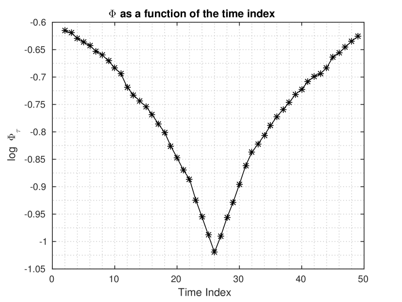
(a) $\Phi_{\tau}$ (as defined in (23)) as a function of the change point $\tau$.

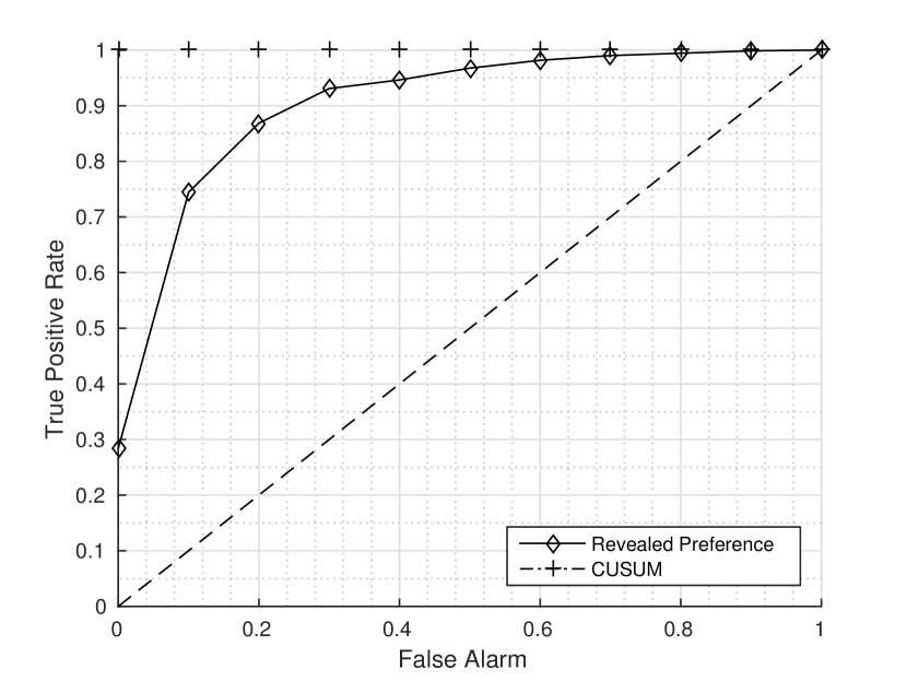
(b) ROC plot.

Figure 2: Estimation of the utility change point using the revealed preference framework (Fig. 2(a)). Fig. 2(b) compares the ROC plots of the revealed preference framework with the CUSUM algorithm. The CUSUM algorithm in Appendix A-G assumes knowledge of the utility function before and after the change point. However, the revealed preference framework considered in this paper assumes no parametric knowledge of the utility function. The plots were generated with $1000$ independent simulations. The parameters of Cobb-Douglas utility $v(x)$ equal to $(a_{1},a_{2})=(0.6,0.4)$ and $\alpha=(1,1)$ with the change point set as $26$. The budget is set to $5$. The noise variance is $0.50$.

V-B Yahoo! Buzz Game

In this section, we present an example of a real dataset of online search process. The objective is to investigate the utility maximization of the online search process and to detect change points at which the utility has changed. The change points give useful information on when the ground truths have changed.

The dataset that we use in our study is the Yahoo! Buzz Game Transactions from the Webscope datasets available from Yahoo! Labs. In 2005, Yahoo! along with O’Reilly Media started a fantasy market where the trending technologies at that point where pitted against each other. For example, in the browser market there were “Internet Explorer”, “Firefox”, “Opera”, “Mozilla”, “Camino”, “Konqueror”, and “Safari”. The players in the game have access to the “buzz”, which is the online search index, measured by the number of people searching on the Yahoo! search engine for the technology. The objective of the game is to use the buzz and trade stocks accordingly. The interested reader is referred to [35] for an overview of the Buzz game. An empirical study of the dataset [36] reveal that most of the traders in the Buzz game follow utility maximization behaviour. Hence, the dataset falls within the revealed preference framework, if we consider the buzz as the probe and the “trading price” as the response to the utility maximizing behaviour.

We consider a subset of the dataset containing only the “WIRELESS” market which contained two main competing technologies: “WIFI” and “WIMAX”. Figure 3 shows the buzz and the “trading price” of the technologies starting from April 1 to April 29. The buzz is published by Yahoo! at the start of each day and the “trading price” was computed as the average of the trading price of the stock for each day.

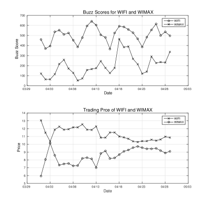
Figure 3: Buzz scores and trading price for WIFI and WIMAX in the WIRELESS market from April 1 to April 29. The change point was estimated as April 18. This corresponds to a new WIFI product announcement. The change can also be observed due to the sudden peak of interest in WIFI around April 18.

Chose the probe and response vector for this dataset as follows

$$p_{t} =\left[\text{Buzz(WIFI)}\quad\text{Buzz(WIMAX)}\right]$$

$$x_{t} =\left[\text{Trading price(WIFI)}\quad\text{Trading price(WIMAX)}\right].$$

Checking the GARP condition or the Afriat inequalities (3), we find that the dataset does not satisfy utility maximization for the entire duration from April 1 to April 29. However, we find that the dataset satisfies utility maximization from April 1 to April 17. Using the inequalities eqs. 6, 7 and 8, that we derived in Sec II, for the model in (5), we see that utility has changed with change point, $\tau$, set to April 18. This correspond to a change in the ground truth which affected the utility of the agents. Indeed, we find that the change point corresponds to Intel’s announcement of WIMAX chip.

Also, by minimizing the 2-norm of the linear perturbation, which we derived in Sec. III, and using the optimization problem, postulated in Sec. II-B, we find that the recovered linear coefficients which correspond to minimum perturbation is $\alpha=[0\;5.9]$. This is inline with what we expect, a positive change in the WIMAX utility, due to the change in ground truth. Furthermore, the recovered utility function, $v(x)$, is shown in Fig. 4(a) and the indifference curve (contour plot) of the base utility is shown in Fig. 4(b).

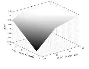
(a)

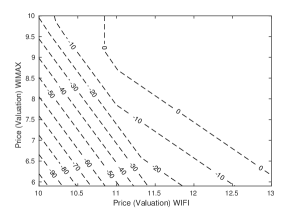
(b)

Figure 4: Fig. 4(a) shows the recovered utility function $v(x)$ using eq. 14. Indifference curve of the recovered utility function, is shown in Fig. 4(b). The indifference curve suggests the substitution behaviour in online search.

The recovered base utility function in Fig. 4(a) satisfy the single crossing conditionindicating strategic substitute behaviour in online search. The substitute behaviour in online search can also be noticed from the indifference curve in Fig. 4(b). This is due to the fact that WIFI and WIMAX were competing technologies for the problem of providing wireless local area network.

V-C Youstatanalyzer Database

We now analyze the utility maximizing behaviour of users engaged in the popular online platform for videos, YouTube. YouTube is an example of a content-aware utility maximization, where the utility depends on the quality of the video present at any point. We measure the quality of the video using two measurable metrics: the number of subscribers and the number of views. The YouTube database that we use for our study is the Youstatanalyzer database. The Youstatanalyzer database is built using the Youstatanalyzer tool [37], which collects statistics of YouTube videos using web scrapping technology. The database is particularly suited for our study of dimensionality reduction in revealed preference, since the entire database contains statistics of 1000K videos.

From the database, we aggregated the statistics of all popular videos existing from start of 08 July, 2012 to end of 07 Sept, 2013, having at least $2$ subscribers. The entire duration was divided into 15 time periods, corresponding to each month of the duration, giving us a total of $15$ observations ($T=15$). The entire duration need to be split into sub-time periods since the statistics of all the videos are not sampled each day. For the revealed preference analysis, each of the dimension of the probe and the response is associated with a unique video ID. The probe for the revealed preference analysis is the number of subscribers and the response is the number of views during the time period. The objective is to investigate utility maximizing behaviour between the number of people subscribed to a particular video and the number of views that the video received. Formally, the probe and the response is chosen as follows:

$$p_{t} =\left[1/\text{\#Subscriber}(\text{Video}{1}),\dots,1/\text{\#Subscriber}(\text{Video}N)\right],$$

$$x_{t} =\left[\text{\#Views}(\text{Video}1),\dots,\text{\#Views}(\text{Video}N)\right].$$

The motivation for this definition is that as the number of subscribers to a video increases, the number of views also increase [38]. The inner product of the probe and the response vector gives the sum of the “view focus” of all videos [39]. Also, a recent study shows that $90\%$ of the YouTube views are due to $20\%$ of the videos uploaded [40]. Hence, if we restrict attention to popular videos, the view focus tend to remain constant during a time period which correspond to the linear constraint in the revealed preference setting.

The number of videos satisfying the above requirements is $7605$, and therefore, the dimension of the probe and response, $m=7605$. The number of inner product computations required for checking the GARP conditions is given by $mT^{2}$. Hence, we apply Johnson-Lindenstrauss lemma to the data using the “database friendly” transform that we presented in Sec IV. We choose $\varepsilon=0.1$, so that the inner product are within 90% of the accuracy. Also, we choose $\beta=0.65$, such that the above condition on the inner products hold with probability at least $0.9$. Substituting the values of $T$, $\varepsilon$ and $\beta$ in (32) we find that the dimension of the embedded subspace is $k=3800$. From the simulations, we see that the GARP is satisfied with probability $0.9$, which is inline with what we expect. For this example, the number of inner product computations required to compute GARP condition in the lower dimensional subspace is given by $kT^{2}$, which is less than the number of computations required to compute the GARP in the original space by a factor of $2$. Note from Lemma IV.1 and Theorem IV.1 that the dimension of the embedding is independent of the dimension of the probe and the response and hence higher computational savings can be obtained when the dimension of the probe and the response are higher.

The utility function obtained in the lower dimension is useful for visualization, and gives a sparse representation of the original utility function. Below, we use the utility function obtained in the lower dimension to predict total traffic to YouTube when the number of subscribers to a particular video changes or when popular YouTube users (people with large number of subscribers) upload new videos. The above approach of predicting total number of views complements the findings in [38], where the authors claim that individual views to YouTube video or channel cannot be predicted. This predicted total traffic serves as an useful benchmark for allocating server resources without compromising the user experience.

Predicting total traffic in YouTube

Based on the utility function recovered in the lower dimension, one can predict the total traffic in YouTube. As before, let $p_{t}\in{\rm IR}^{m}$ and $x_{t}\in{\rm IR}^{m}$ be the number of subscribers and the number of views at time $t$, respectively. Let $\tilde{p_{t}}\in{\rm IR}^{k}$ and $\tilde{x_{t}}\in{\rm IR}^{k}$ be the lower dimensional embedding of $p_{t}$ and $x_{t}$, respectively. The total traffic, or the number of views, at time $t$, is given by $T_{t}=\sum_{i=1}^{m}x_{t}^{i}$.

We can estimate the total traffic using the lower dimension utility function. Given $p$, the number of subscribers at time $t+1$, let $\tilde{p}$ denote the lower dimensional embedding of $p$. The corresponding value of $\tilde{x}$ that rationalizes the data can be obtained by solving the following optimization problem:

$$\tilde{x}=\underset{\{\tilde{p}^{\prime}x\leq I\}}{\operatorname{argmax}}\underset{i\in\left\{1,2,\dots,t\right\}}{\operatorname{min}}\{u_{i}+\lambda_{i}\tilde{p_{i}}^{\prime}(x-\tilde{x_{i}})\},$$ (34)

The values of $\left\{u_{i},\lambda_{i}\right\}$ are such that the GARP condition (3) is satisfied for the dataset $\left\{(\tilde{p_{i}},\tilde{x_{i}})_{i=1,2,\dots,t}\right\}$. The budget $I$, is assumed to be known or estimated independently of the above optimization problem. The estimated traffic due to the probe $\tilde{p}$ is given by $\tilde{T}=\sum_{i=1}^{k}\tilde{x}^{i}$.

VI Conclusion

This paper derived a revealed preference based approach for change point detection in the utility function. The main result (Theorem II.2) provided necessary and sufficient conditions for the existence of the change point at which the utility function jump changes by a linear perturbation. In addition, in the presence of noise, we provided a procedure for detecting the unknown change point and a hypothesis test for testing the dataset for dynamic utility maximization. The results were applied on the Yahoo! Tech Buzz dataset and the estimated change point corresponds to the change in ground truth.

The application of results developed in this paper provided novel insights into the utility maximizing behaviour of agents in online social media. Extension of the current work could involve analytically characterizing the GARP failure rate due to dimensionality reduction, or considering multiple change points, or considering higher order perturbation functions.

References

- [1] B. Reeves and C. Nass, How people treat computers, television, and new media like real people and places. CSLI Publications and Cambridge university press, 1996.
- [2] O. Toubia and A. T. Stephen, “Intrinsic vs. image-related utility in social media: Why do people contribute content to twitter?” Marketing Science, vol. 32, no. 3, pp. 368–392, 2013.
- [3] P. Samuelson, “A note on the pure theory of consumer’s behaviour,” Economica, vol. 5, no. 17, pp. 61–71, 1938.
- [4] S. Afriat, “The construction of utility functions from expenditure data,” International economic review, vol. 8, no. 1, pp. 67–77, 1967.
- [5] H. Varian, “The nonparametric approach to demand analysis,” Econometrica, vol. 50, no. 1, pp. 945–973, 1982.
- [6] W. Diewert, “Afriat and revealed preference theory,” The Review of Economic Studies, vol. 40, no. 3, pp. 419–425, 1973.
- [7] H. Varian, “Revealed preference,” Samuelsonian economics and the twenty-first century, pp. 99–115, 2006.
- [8] V. Krishnamurthy and W. Hoiles, “Afriat’s test for detecting malicious agents,” IEEE Signal Processing Letters, vol. 19, no. 12, pp. 801–804, 2012.
- [9] M. Barni and F. Pérez-González, “Coping with the enemy: Advances in adversary-aware signal processing,” in IEEE Conf. on Acoustics, Speech and Signal Processing, 2013, pp. 8682–8686.
- [10] W. Hoiles and V. Krishnamurthy, “Nonparametric demand forecasting and detection of energy aware consumers,” IEEE Transactions on Smart Grid, vol. 6, no. 2, pp. 695–704, March 2015.
- [11] S. Currarini, M. O. Jackson, and P. Pin, “Identifying the roles of race-based choice and chance in high school friendship network formation,” Proc. of the National Academy of Sciences, vol. 107, no. 11, pp. 4857–4861, 2010.
- [12] R. K.-X. Jin, D. C. Parkes, and P. J. Wolfe, “Analysis of bidding networks in eBay: aggregate preference identification through community detection,” in Proc. of AAAI workshop on PAIR, 2007.
- [13] J. Strebel, T. Erdem, and J. Swait, “Consumer search in high technology markets: exploring the use of traditional information channels,” Journal of Consumer Psychology, vol. 14, no. 1, pp. 96–104, 2004.
- [14] J. Ginsberg, M. H. Mohebbi, R. S. Patel, L. Brammer, M. S. Smolinski, and L. Brilliant, “Detecting influenza epidemics using search engine query data,” Nature, vol. 457, no. 7232, pp. 1012–1014, 2009.
- [15] H. A. Carneiro and E. Mylonakis, “Google trends: A web-based tool for real-time surveillance of disease outbreaks,” Clinical Infectious Diseases, vol. 49, no. 10, pp. 1557–1564, 2009.
- [16] X. Zhou, J. Ye, and Y. Feng, “Tuberculosis surveillance by analyzing google trends,” IEEE Trans. on Biomedical Engineering, vol. 58, no. 8, pp. 2247–2254, Aug 2011.
- [17] A. Seifter, A. Schwarzwalder, K. Geis, and J. Aucott, “The utility of “google trends” for epidemiological research: Lyme disease as an example,” Geospatial Health, vol. 4, no. 2, pp. 135–137, 2010.
- [18] J. A. Doornik, “Improving the timeliness of data on influenza-like illnesses using google trends,” Tech. Rep., 2010.
- [19] L. Wu and E. Brynjolfsson, The Future of Prediction: How Google Searches Foreshadow Housing Prices and Sales. University of Chicago Press, 2009, p. 147.
- [20] A. Tumasjan, T. Sprenger, P. Sandner, and I. Welpe, “Predicting elections with twitter: What 140 characters reveal about political sentiment,” in Int. AAAI Conference on Web and Social Media, 2010, pp. 178–185.
- [21] B. K. Kaye and T. J. Johnson, “Online and in the know: Uses and gratifications of the web for political information,” Journal of Broadcasting & Electronic Media, vol. 46, no. 1, pp. 54–71, 2002.
- [22] A. Adams, R. Blundell, M. Browning, and I. Crawford, “Prices versus preferences: taste change and revealed preference,” Mar 2015. [Online]. Available: /uploads/publications/wps/WP201511.pdf
- [23] D. L. McFadden and M. Fosgerau, “A theory of the perturbed consumer with general budgets,” National Bureau of Economic Research, Tech. Rep., 2012.
- [24] D. J. Brown and R. L. Matzkin, “Estimation of nonparametric functions in simultaneous equations models, with an application to consumer demand,” 1998.
- [25] D. Fudenberg, R. Iijima, and T. Strzalecki, “Stochastic choice and revealed perturbed utility,” Econometrica, vol. 83, no. 6, pp. 2371–2409, 2015.
- [26] G. C. Chasparis and J. Shamma, “Control of preferences in social networks,” in Decision and Control (CDC), IEEE Conf. on, Dec 2010, pp. 6651–6656.
- [27] M. Basseville and I. Nikiforov, Detection of Abrupt Changes — Theory and Applications, ser. Information and System Sciences Series. New Jersey, USA: Prentice Hall, 1993.
- [28] M.-F. Balcan, A. Daniely, R. Mehta, R. Urner, and V. V. Vazirani, “Learning economic parameters from revealed preferences,” in Int. Conf. on Web and Internet Economics. Springer, 2014, pp. 338–353.
- [29] M. Zadimoghaddam and A. Roth, “Efficiently learning from revealed preference,” in Internet and Network Economics. Springer, 2012, pp. 114–127.
- [30] E. Beigman and R. Vohra, “Learning from revealed preference,” in Proc. of the 7th ACM Conference on Electronic Commerce, ser. EC ’06, 2006, pp. 36–42.
- [31] O. Chapelle, B. Schlkopf, and A. Zien, Semi-Supervised Learning, 1st ed. The MIT Press, 2010.
- [32] W. B. Johnson and J. Lindenstrauss, “Extensions of Lipschitz mappings into a Hilbert space,” Contemporary mathematics, vol. 26, pp. 189–206, 1984.
- [33] D. Achlioptas, “Database-friendly random projections: Johnson-lindenstrauss with binary coins,” Journal of Computer and System Sciences, vol. 66, pp. 671–687, 2003.
- [34] S. S. Vempala, The random projection method. American Mathematical Soc., 2005, vol. 65.
- [35] B. Mangold, M. Dooley, G. Flake, H. Hoffman, T. Kasturi, D. Pennock, and R. Dornfest, “The Tech Buzz Game,” Computer, vol. 38, no. 7, pp. 94–97, July 2005.
- [36] Y. Chen, D. M. Pennock, and T. Kasturi, “An empirical study of dynamic pari-mutuel markets: Evidence from the tech buzz game,” in Proc. of WebKDD, 2008.
- [37] M. Zeni, D. Miorandi, and F. D. Pellegrini, “Youstatanalyzer: A tool for analysing the dynamics of YouTube content popularity,” in Proc. of the 7th Intn. Conf. on Performance Evaluation Methodologies and Tools, 2013, pp. 286–289.
- [38] X. Cheng, M. Fatourechi, X. Ma, C. Zhang, L. Zhang, and J. Liu, “Insight data of YouTube from a partner’s view,” in Proc. of NOSSDAV Workshop. ACM, 2014, pp. 73–78.
- [39] A. Brodersen, S. Scellato, and M. Wattenhofer, “YouTube around the world: Geographic popularity of videos,” in Proc. of the 21st Int. Conf. on World Wide Web, ser. WWW ’12. ACM, 2012, pp. 241–250.
- [40] Y. Ding, Y. Du, Y. Hu, Z. Liu, L. Wang, K. Ross, and A. Ghose, “Broadcast yourself: Understanding YouTube uploaders,” in Proc. of SIGCOMM Conf. on Internet Measurement Conference, 2011, pp. 361–370.
- [41] M. Gerasimov, V. Kruglov, and A. Volodin, “On negatively associated random variables,” Lobachevskii Journal of Mathematics, vol. 33, no. 1, pp. 47–55, 2012.
- [42] K. Joag-Dev and F. Proschan, “Negative association of random variables with applications,” The Annals of Statistics, pp. 286–295, 1983.