Semi-classical analysis of black holes in Loop Quantum Gravity:
Modelling Hawking radiation with volume fluctuations

Abstract

We introduce the notion of fluid approximation of a quantum spherical black hole in the context of Loop Quantum Gravity. In this limit, the microstates of the black hole are intertwiners between “large” representations $s_{i}$ which typically scale as $s_{i}\sim\sqrt{a_{H}}$ where $a_{H}$ denotes the area of the horizon in Planck units. The punctures with large colors are, for the black hole horizon, similar to what are the fluid parcels for a classical fluid. We dub them puncels. Hence, in the fluid limit, the horizon is composed by puncels which are themselves interpreted as composed (in the sense of the tensor product) by a large number of more fundamental intertwiners. We study the spectrum of the euclidean volume acting on puncels and we compute its quantum fluctuations. Then, we propose an interpretation of black holes radiation based on the properties of the quantum fluctuations of the euclidean volume operator. We estimate a typical temperature of the black hole and we show that it scales as the Hawking temperature.

I Introduction

The last twenty years, several approaches have been developed in the framework of Loop Quantum Gravity to describe black hole microstates which are responsible for their huge entropy and to explain more generally their famous thermodynamical properties Bekenstein ; Hawking . After the first heuristic but seminal model of black holes in Loop Quantum Gravity Rovelli , one introduced the idea of isolated horizons Ash0 ; Ash1 ; Ash2 ; Ash3 which allowed for a very clear description of the black hole microstates in terms of a Chern-Simons theory Ash4 ; Ash5 ; BHentropy8 ; BHentropy6 . Most of these models have in common that counting the microstates leads to recovering the Bekenstein-Hawking law only when the Barbero-Immirzi parameter $\gamma$ is fixed to a special value. The fact that $\gamma$ plays such an important role has raised some doubts and criticisms about the way we describe black holes in Loop Quantum Gravity. However, a new perspective has been opened the last years BHentropy8 ; BHentropy6 showing that it is possible to fix $\gamma=\pm i$ to compute black holes entropy which reproduces exactly the Bekenstein-Hawking law at the semi-classical limit. This result suggests that the quantum theory, when described in terms of self dual variables Ashtekar:1986yd , might automatically account for a right description of quantum black holes. See Alereview for a complete recent review on black holes in Loop Quantum Gravity.

If the entropy and the microstates of black holes has been studied a lot, very few models about Hawking radiation in Loop Quantum Gravity were developed. The quasi-local approach GhoshAle1 ; GhoshAle2 allowed to introduce the notion of temperature; in Bianchi rad , one made used of this temperature to develop a model of radiation in the context of Spin-Foam models; in radiation radiation has been explained from a group theoretical point of view in canonical Loop Gravity. However, none of these models really propose a full and dynamical fundamental explanation of the Hawking radiation. We propose and explore an idea to make progress in this direction. It consists in assuming that the black hole radiation originates from quantum fluctuations of its horizon. Hence, we study some properties of these fluctuations at the semi-classical level from the properties of the spectrum of the euclidean volume operator acting on the space of black hole microstates. Then, we show that they could be interpreted in terms of defects spread on the horizon, and the typical length $\lambda$ between two such defects scales as $\sqrt{a_{H}}$ where $a_{H}$ is the area of the horizon. Then, we argue that $\lambda$ could be viewed as a fundamental wavelength of the black hole and one shows that it corresponds to a temperature $T$ which naturally scales as the Hawking temperature.

To construct this model, first we introduce the concept of fluid approximation for a black hole in Loop Quantum Gravity. This approximation consists in considering only a particular class of “semi-classical” states for the black hole. This class is such that the representations coloring the punctures which cross the horizon are semi-classical (they scale as $\sqrt{a_{H}}$ in Planck units according to Noui2 ), and the intertwiners describing the microstates are restricted to a particular cathegory. These intertwiners are associated to a graph $\Gamma$ dual to a triangulation $\Delta$ of the ball as shown in figure 1. Hence, they are obtained by contracting together $n$ 4-valent intertwiners between large representations. These 4-valent intertwiners are for the black hole what parcels are for a fluid, and we dub them puncels. To understand thermodynamical aspects of the black hole in the fluid limit, we proceed as one usually does for the calculation of black holes path integral: we transform the lorentzian geometry into a euclidean one, hence the black hole is transformed into a 3-ball whose boundary is the horizon. We show that the properties of the quantum geometry of this 3-ball allows us to interpret the Hawking radiation from the point of view of Loop Quantum Gravity. Indeed, we compute the semi-classical spectrum of the euclidean volume operator acting on the semi-classical states, and we interpret volume fluctuations in terms of deformations of the black hole horizon. Finally, as we said above, we can easily interpret these deformations as defects which are spread on the horizon with a typical length $\lambda\sim\sqrt{a_{H}}$. Note that we mostly work in the model where $\gamma=\pm i$ (the representations are continuous) but our analysis could be adapted to the case $\gamma\in\mathbb{R}$.

The paper is organized as follows. Section II is devoted to define the fluid approximation of the black hole. In Section III, we compute the spectrum of the volume operator in the fluid approximation, and we relate the volume fluctuations to the Hawking radiation. We conclude in Section IV with a discussion on this model.

II Black Holes in the fluid approximation

In this section, we introduce the concept of fluid limit of a spherical black hole. We first recall some fundamental properties of $SU(2)$ black holes in the context of Loop Quantum Gravity. Then, we define their fluid approximation.

II.1 Black Holes and $SU(2)$ Chern-Simons theory

It is well-known that the quantum microstates of a spherical black hole are those of an $SU(2)$ Chern-Simons theory on a punctured 2-sphere $S^{2}$ BHentropy8 ; BHentropy6 ; BHentropy7 . Let us quickly recall how this works.

II.1.1 Microstates are intertwiners

Even though $S^{2}$ is a topological sphere (with no geometrical structure), it represents the horizon of the black hole from a classical point of view. The punctures have a quantum nature and originate from those edges of quantum geometry states which cross the horizon. They are a priori colored with spins $j$ and they carry quanta of area $a_{j}=8\pi\gamma\ell_{p}^{2}\sqrt{j(j+1)}$ where $\gamma$ is the Barbero-Immirzi parameter and $\ell_{p}$ the Planck length. Hence, the Hilbert space of quantum black hole microstates is given by

$$\bigoplus_{(n_{j})\in\,{\cal C}(a_{H})}\text{Int}(\bigotimes_{j=1}^{\infty}V_{j}^{\otimes n_{j}})$$ (1)

where $V_{j}$ denotes the (modulus of the) spin $j$ representation of dimension $d_{j}=2j+1$, $n_{j}$ is the number of punctures colored with $j$, and we have introduced the constraint ${\cal C}(a_{H})$

$$a_{H}-8\pi\ell_{p}^{2}\gamma\sum_{j}n_{j}\sqrt{j(j+1)}=0$$ (2)

which ensures that the area of the horizon is fixed to $a_{H}$. In fact, this description of the space of microstates has already taken into account that the black hole is semi-classical in the sense that $a_{H}\gg\ell_{p}^{2}$. When the black hole is “smaller”, we must consider quantum corrections. In fact, classical $SU(2)$ intertwiners are replaced by quantum intertwiners, more precisely by intertwiners of the quantum group $U_{q}(su(2))$ where $q$ is a root of unity. Details can be found in BHentropy7 .

II.1.2 Number of microstates and semi-classical limit: $\gamma\in\mathbb{R}$

The dimension ${\cal N}(a_{H})$ of the space of states (1) can be computed easily from group theory techniques. It is formally given by

$${\cal N}(a_{H})=\sum_{{\cal C}(a_{H})}\text{dim}[\text{Int}(\bigotimes_{j=1}^{\infty}V_{j}^{\otimes n_{j}})]$$ (3)

where the sum runs over the configurations of spins $(n_{j})$ which satisfy ${\cal C}(a_{H})$ and

$$\text{dim}[\text{Int}(\bigotimes_{j=1}^{\infty}V_{j}^{\otimes n_{j}})]\;=\;\frac{2}{\pi}\int_{0}^{\pi}d\theta\,\sin^{2}\theta\,\prod_{j}\left(\frac{\sin(d_{j}\theta)}{\sin\theta}\right)^{n_{j}}$$ (4)

is the number of invariant tensors in the tensor product $\otimes_{j}(V_{j}^{\otimes n_{j}})$. Many different methods have been developed to compute the first terms of the semi-classical expansion ($a_{H}\gg\ell_{p}^{2}$) of ${\cal N}(a_{H})$ Rovelli ; kaulma1 ; kaulma2 ; kaulma3 ; counting1 ; counting2 ; counting3 ; counting4 ; counting5 ; BHentropy3 ; Liv1 ; Bianchi . One shows that it reproduces the Bekenstein-Hawking law at the leading order provided that $\gamma$ is fixed to a particular numerical value $\gamma_{0}$, i.e.

$$S(a_{H})\equiv\ln{\cal N}(a_{H})=\frac{\gamma_{0}}{\gamma}\frac{a_{H}}{4\ell_{p}^{2}}-\frac{3}{2}\ln\left(\frac{a_{H}}{\ell_{p}^{2}}\right)+\cdots$$ (5)

The explicit value of $\gamma_{0}$ can be computed numerically (see BHentropy7 for example). Note that the punctures are assumed to behave as distinguishable particles to obtain the Bekenstein-Hawking law. Furthermore, the semi-classical limit can be shown to be dominated by configurations where the spins are small in the sense that the mean color and then the mean number of punctures when the black hole is macroscopic are given by:

$${1}/{2}<\langle j\rangle<1\qquad\text{and}\qquad\langle n\rangle=n_{0}\frac{a_{H}}{\ell_{p}^{2}}\,,$$ (6)

where $n_{0}$ is a constant. The means are computed in the microcanonical ensemble according to the partition function (3).

II.1.3 Analytic continuation to $\gamma=\pm i$

It goes without saying that the strong dependence of the black hole entropy computation on $\gamma$ has remained a controversial aspect. The first reason is that the Barbero-Immirzi parameter plays no role at the semi-classical level whereas it is crucial at the quantum level, at least in the understanding of black holes entropy. Second, the value of $\gamma_{0}$ (5) for some models of rotating black holes is different from the one computed in the case of spherical black holes Ale2 ; rotating . All these results strongly suggest to look at alternative methods to understand thermodynamical properties of black holes in Loop Quantum Gravity.

A first promising perspective on the issue of the dependence of black holes entropy in $\gamma$ was put forward thanks to the availability of the canonical ensemble formulation of the entropy calculation making use of the quasi-local description of black holes GhoshAle1 ; GhoshAle2 ; GhoshAle3 . Before, most of the calculations had been performed in the microcanonical ensemble and then, they were reduced to a calculation of number of microstates. The introduction of a notion of quasi-local energy $E(n_{j})$ for black holes microstates enabled us to compute a canonical (and eventually a grand canonical) partition function ${\cal Z}(\beta)$ where $\beta$ is the inverse temperature GhoshAle3 . It is formally defined by

$${\cal Z}(\beta)=\sum_{(n_{j})}\mu(n_{j})\exp[-\beta E(n_{j})]$$ (7)

where the sum runs over all possible microscopic configurations $(n_{j})$ satisfying ${\cal C}(a_{H})$. The measure $\mu$ takes into account the matter sector and the symmetrisation factors. It was shown in GhoshAle3 that the semi-classical analysis of the partition function allows to recover the right semi-classical behavior for all values of $\gamma$. The semi-classical limit occurs at the vicinity of the Unruh temperature $\beta_{u}$ (defined for the “quasi-local” observer in the context of the “quasi-local” description of black holes) where the entropy behaves as

$$S(\beta_{u})=\ln{\cal Z}(\beta_{u})-\beta_{u}\frac{\partial\ln{\cal Z}}{\partial\beta}(\beta_{u})=\frac{a_{H}}{4\ell_{p}^{2}}+\cdots$$ (8)

More precisely, the entropy of large semiclassical black holes coincides with the Bekenstein-Hawking law at the leading order, while the dependence on the Immirzi-Barbero parameter is shifted to sub-leading quantum corrections. In this approach, the semi-classical limit is dominated by large spins in the sense that the mean color and the mean number of punctures generically scale as

$$\langle j\rangle\approx\sigma\frac{\sqrt{a_{H}}}{\ell_{p}}\,\qquad\text{and}\qquad\langle n\rangle\approx\nu\frac{\sqrt{a_{H}}}{\ell_{p}}\,.$$ (9)

Here $\sigma$ and $\nu$ are constant, and the means are computed in the grand canonical ensemble. We assumed that the punctures satisfy the Bose-Einstein or the Maxwell-Boltzmann statistic in the semi-classical regime. A similar result exists for the Fermi-Dirac statistic GhoshAle3 .

Another perspective to understand the semi-classical limit of spherical black holes which relies on analytic continuation techniques was originally proposed in Noui1 . This idea was developed further in Noui2 ; Noui0 ; JBA1 . It was adapted to three-dimensional BTZ black holes in BTZ , it was recently generalized to models of rotating black holes in rotating , and it was also applied to explain Hawking radiation radiation from group theory arguments. Note that this idea is strongly supported by different complementary approaches in different contexts J1 ; J2 ; Pranz1 ; Pranz2 ; Pranz3 ; Ale1 ; Yasha1 ; Yasha2 ; BN ; Muxin . In all these cases, the number of microstates (viewed as a function of the parameter $\gamma$) is analytically continued from $\gamma\in\mathbb{R}$ to $\gamma\in\mathbb{C}$ and then evaluated at the special complex values $\gamma=\pm i$. A simple analysis shows that it grows asymptotically as $\exp(a_{H}/(4\ell_{p}^{2}))$ for large areas. The result is striking in that these values of the Immirzi parameter are special in the connection formulations of gravity: they lead to the simplest covariant parametrization of the phase space of general relativity in terms of the so-called Ashtekar variables Ashtekar:1986yd . Moreover, this suggests that the quantum theory, when defined in terms of self dual variables, might automatically account for a holographic degeneracy of the area spectrum of the black hole horizon. The main differences with the real $\gamma$ description of black holes is that, first, the horizon area has now a continuous spectrum, and second the semi-classical limit is dominated by large representations. Indeed, each spin $j$ coloring the punctures are mapped into the complex number $j\mapsto 1/2(-1+is)$ which depends on the real parameter $s$. In that way, quanta of area remain real when $\gamma$ takes the values $\gamma=\pm i$

$$a_{j}=8\pi\gamma\ell_{p}^{2}\sqrt{j(j+1)}\longmapsto a_{j}=4\pi\ell_{p}^{2}\sqrt{s^{2}+1}\qquad\text{with}\quad\gamma=\pm i\,,\,\,j=\frac{1}{2}(-1+is)\,.$$ (10)

Generically (when the particles satisfy the Maxwell-Boltzmann statistics at the semi-classical limit), the mean representation and the mean number of punctures were shown to scale exactly as (9) in the semi-classical regime Noui2 . Hence, these conclusions coincide with the analysis of the partition function using the quasi-local energy GhoshAle3 (briefly recalled above) with the difference that discrete spins are replaced by continuous representations. It is interesting to emphasize once more that the analytic continuation method was successfully adapted to models of rotating black holes rotating : the entropy of a rotating black hole reproduces the expected semi-classical law when $\gamma=\pm i$ whereas this is clearly not the case when $\gamma$ is real.

II.2 Fluid approximation and fluid “puncels”

From now on, we consider the model based on the analytic continuation where the semi-classical limit is dominated by large continuous representations. This model is more satisfying than the others mainly because it leads to a $\gamma$-independent semi-classical behavior of the black hole entropy (at least at the leading order). Furthermore, contrary to the model based on the quasi-local approach, no assumption on the matter sector is required to recover the Bekenstein-Hawking formula. Note however that adapting the notion of fluid approximation to the quasi-local formulation of black holes is straightforward.

II.2.1 The fluid approximation

It is therefore natural to expect that black holes microstates are more likely described as intertwiners between large representations when the black hole is macroscopic. Hence, we will assume that only these “large” intertwiners play an important role to understand and to explain some semi-classical properties of black holes. As a consequence, we will restrict ourselves to the subspace of such microstates (with large representations) to describe semi-classical black holes. We dub these states fluid “puncels” in analogy with fluid mechanics where a fluid, in the hydrodynamic regime, is understood as a system of interacting fluid parcels. A fluid parcel is a small amount of fluid which contains a large number of molecules. This is very similar to fluid puncels for black holes which are a small amount of horizon which can be understood as a tensor product of a large amount of more fundamental representations. Studying the black hole in terms of fluid puncels instead of more fundamental intertwiners defines what we call the fluid approximation.

II.2.2 Puncels

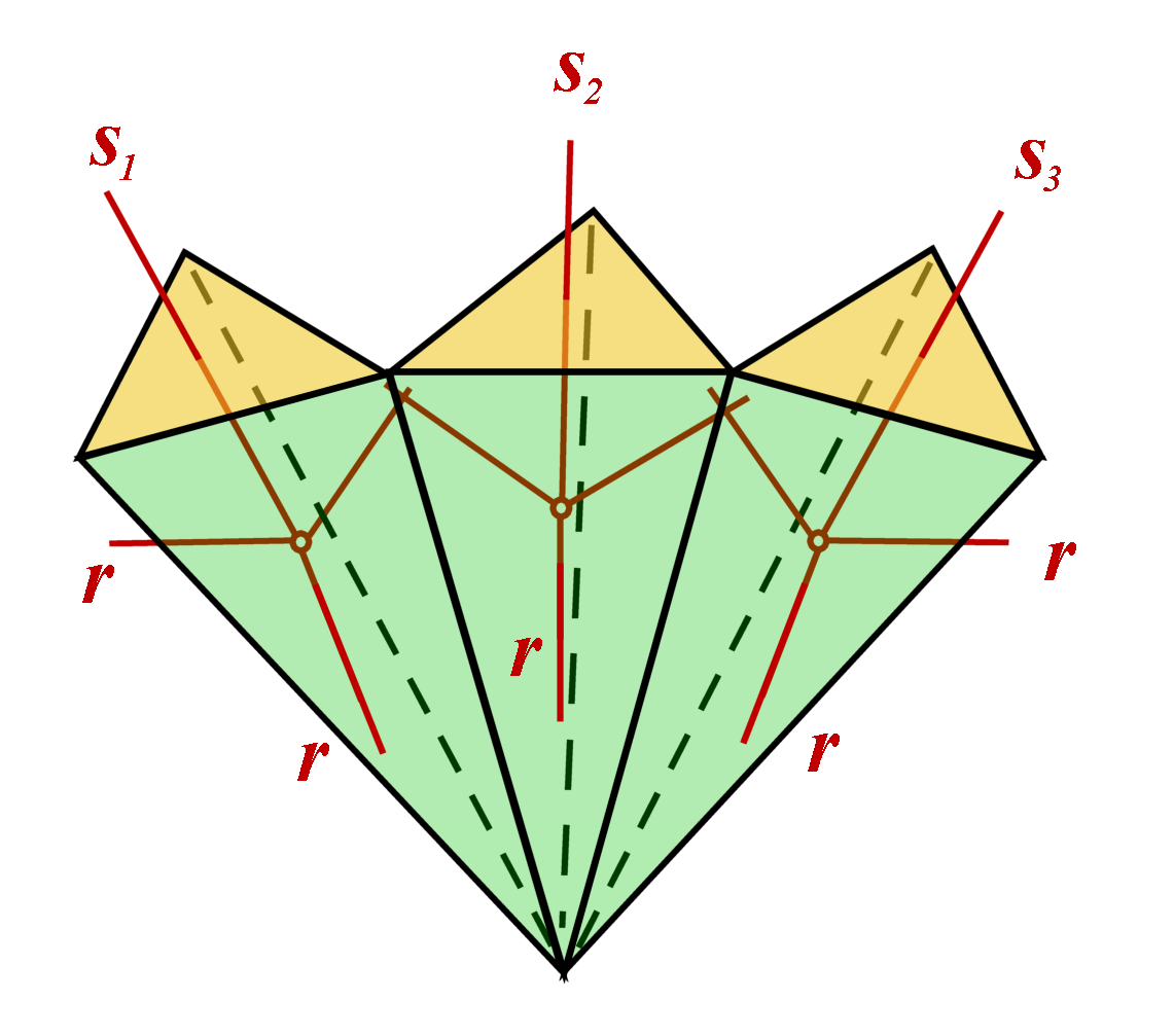
Figure 1: Representation of three puncels of a black hole in fluid approximation. Each tetrahedron is composed by 3 (green) triangles inside the horizon ($\tau^{I}$) and 1 (yellow) traingle on the horizon $\tau^{H}$. Only a part of the triangulation $\Delta$ (black lines) and the corresponding dual graph $\Gamma$ (red lines) are represented here. The dual graph is associated to an intertwiner between the representations $s_{1},s_{2},s_{3},\cdots$.

Let us propose a more precise definition of the black hole in the fluid representation. Its microstates satisfy the following properties.

1. They are intertwiners between $n$ large representations $s_{i}\propto\sqrt{a_{H}}/\ell_{p}$ (or $j_{i}\propto\sqrt{a_{H}}$ in the quasi-local approach). Hence they belong to the space $\text{Int}(\otimes_{i}V_{s_{i}})$.

2. They are decomposed into $4$-valent intertwiners (inside the horizon) in a way that they are associated to a 4-valent complex $\Gamma$ which is assumed to be dual to a triangulation $\Delta=\Gamma^{*}$ of a three dimensional ball whose boundary is the horizon.

3. Each tetrahedron $T$ of the triangulation $\Delta$ is associated to a 4-valent intertwiner of the form

   $$\iota:V_{s}\otimes V_{r_{1}}\otimes V_{r_{2}}\otimes V_{r_{3}}\rightarrow\mathbb{C}$$ (11)

   where $s$ colors the face on the horizon and $r_{i}$ color all the faces inside the hole.

Puncels are represented in the picture 1. As a consequence, a semi-classical state of a black hole (in the fluid approximation) with horizon $a_{H}$ is determined by a family of representations $(s_{\ell},r_{\ell_{1}},r_{\ell_{2}},r_{\ell_{3}})$ and by a family of $n$ intertwiners of the type (11). The colors $(s_{\ell},r_{\ell_{1}},r_{\ell_{2}},r_{\ell_{3}})$ represent the area of the triangles $\tau_{\ell}^{H}$ on the horizon and $\tau_{\ell j}^{I}$ ($j=1,2,3$) inside the hole which are boundaries of the tetrahedron $T_{\ell}$ according to

$$\text{Area}(\tau_{\ell}^{H})=4\pi\ell_{p}^{2}s_{\ell}\,\qquad\text{and}\qquad\text{Area}(\tau_{\ell_{j}}^{I})=4\pi\ell_{p}^{2}r_{\ell j}\,.$$ (12)

When all the representations $s_{\ell}$ are equal to $s$ and $r_{\ell j}=r$, we say that the decomposition of the black hole in terms of puncels is fully symmetric. In that case, the number $n$ of fully symmetrized puncels of the black hole is trivially given by

$$n=\frac{1}{4\pi\sigma}\,\frac{\sqrt{a_{H}}}{\ell_{p}^{2}}\,.$$ (13)

When we study the semi-classical properties of the black hole, we will limit ourselves to semi-classical microstates which are close to fully symmetric states. Only those states which are close to being fully symmetric allow to understand semi-classical properties of black holes. In that case, we will assume that the colors $r_{\ell i}$ inside the hole are all identical to the same value denoted $r$ with no index in the sequel. From now on, we will only consider such states.

III Black Hole spectrum and volume fluctuations

This part is devoted to introduce and study a model of Hawking radiation using the fluid approximation of black holes. In this model, the radiation is closely linked to quantum fluctuations of the euclidean volume operator associated to the black hole. Indeed, we proceed as in the approaches based on a calculation of the path integral: we transform lorentzian metrics into euclidean ones. In the path integral context, this is done using a Wick rotation. In our context, we transform the geometry inside the horizon by an euclidean geometry. Hence, the euclidean black hole appears as a euclidean three-ball whose boundary is the horizon. This (kind of) Wick transformation allows us to interpret the puncels as quantum tetrahedra and the fluid approximation as a discretization of the black hole in terms of quantum tetrahedra. We will make use of this euclidean transformation to understand some aspects of black holes radiation in the context of Loop Quantum Gravity.

For this reason, we study, in the first subsection, the action of the volume operator on black hole microstates in the fluid approximation. Then, in a second subsection, we deduce the spectrum of the volume in this limit. Finally, in the last subsection, we relate the volume fluctuations to the black hole radiation. In particular, we develop a simple model for the radiation based on the fluid approximation of black holes. This model enables us to show that, if we assume that black holes radiate a thermal spectrum, its temperature $T$ scales necessarily as the Hawking temperature.

III.1 Volume of the Euclidean black hole

At the quantum level, microstates in the fluid approximation are $n$-valent intertwiners $\iota(s_{1},\cdots,s_{n})$ between the representations $s_{\ell}$ which is decomposed as the (tensorial) contraction between $n$ puncels (11). We can formally write it as

$$\iota(s_{1},\cdots,s_{n})=\langle\!\langle\otimes_{\ell=1}^{n}\iota_{\ell}(s_{\ell},r,r,r)\rangle\!\rangle_{\Gamma}$$ (14)

where the notation $\langle\!\langle\cdot\rangle\!\rangle_{\Gamma}$ means that internal indices are contracted according to the graph $\Gamma$ depicted in figure 1.

III.1.1 Volume operator: definition and matrix elements in the fluid approximation

A priori, only $\iota(s_{1},\cdots,s_{n})$, such that $j_{k}=1/2(-1+is_{k})$ and $\ell=1/2(-1+ir)$ are integers, are well-defined because they correspond to $SU(2)$ intertwiners. When $s_{k}$ and $\ell$ are real, one could interpret $\iota(s_{1},\cdots,s_{n})$ as an $SU(1,1)$ intertwiner between representations in the principal series. However, such intertwiners need a regularization to be well-defined due to the non-compactness of $SU(1,1)$. Moreover, it is not clear how to compute for instance the action of the volume operator $\hat{V}$ (which is intrinsically an $SU(2)$ operator) on $SU(1,1)$ intertwiners. For these reasons, we define the state (14) in an indirect way: for any operator $\hat{O}$ acting on the space of intertwiners (1) endowed with the scalar product $\langle\cdot|\cdot\rangle$, the matrix elements

$$\langle\iota(s^{\prime}_{1},\cdots,s^{\prime}_{n})|\hat{O}|\iota(s_{1},\cdots,s_{n})\rangle$$ (15)

is defined as the analytic continuation of the corresponding $SU(2)$ matrix element according to the analytic continuation rules (10).

The action of the volume operator on the space of $SU(2)$ $n$-valent intertwiners has been deeply studied in thiemann . Its matrix elements which involve (6j)-symbols are very complicated coefficients. A part from numerical analysis, such a general formula would be totally useless for our purposes. It is even not obvious that the analytic continuation of these coefficients makes sense. Fortunately, as we are going to argue, we expect the action of the volume operator to simplify in the fluid approximation.

At first sight, the space of black holes intertwiners (14) in the fluid limit is clearly not stable under the action of the volume operator $\hat{V}$ and we have

$$\hat{V}|\iota\rangle=\sum_{\iota^{\prime}}\langle\iota^{\prime}|\hat{V}|\iota\rangle\,|\iota^{\prime}\rangle+\sum_{\omega}\langle\omega|\hat{V}|\iota\rangle\,|\omega\rangle$$ (16)

where the first sum runs over an orthonormal basis of (14) and the second one runs over intertwiners $\omega$ orthogonal to (14). However, we expect that the second term in (16) to be negligible compared to the first one in the fluid approximation. The reason is that, as we are going to see, the first term in (16) contains itself the right classical limit for the volume operator. Then the rest are only quantum corrections to the volume in the fluid approximation. We will neglect them. Furthermore, we conjecture that the action of the volume operator simplifies further and can be reduced to the following form

$$\hat{V}\iota(s_{1},\cdots,s_{n})=\sum_{j=1}^{n}\langle\!\langle\iota_{1}(s_{1})\otimes\cdots\otimes[\hat{V}\iota_{j}(s_{j})]\otimes\cdots\otimes\iota_{n}(s_{n})\rangle\!\rangle_{\Gamma}+\,\varepsilon$$ (17)

where $\varepsilon$ stands for terms which are also negligible in the fluid approximation. The reason is the same as the previous one. Indeed, the semi-classical of the first term in the expression of the volume operator

$$\hat{V}{}^{(sc)}=\sum_{j=1}^{n}\mathbb{I}\otimes\cdots\otimes\hat{V}_{4}\otimes\cdots\otimes\mathbb{I}$$ (18)

acting on (14) can be shown to lead to the right classical limit. We used the notation $\mathbb{I}$ for the identity and $\hat{V}_{4}$ for the 4-valent volume operator acting on one puncel only.

As a conclusion, we will decompose the volume operator as a direct sum of independent 4-valent volume operators $\hat{V}_{4}$ acting on each puncel of the black hole. Obviously, this approximation drastically simplifies the analysis of the volume operator on the black hole microstates in the fluid limit.

III.1.2 Volume operator acting on a puncel

It remains to compute the action of the 4-valent volume operator $\hat{V}_{4}$ on a puncel $\iota(s_{j})$. Instead of starting with the general expression, we first simplify the expression of the classical volume of a puncel, then we quantize it and only then we compute its action. Notice that, in the following subsection, we will start with the general expression of $\hat{V}_{4}$ and we will show how its action on puncels is related to the calculation of this subsection.

It is immediate to show that the classical volume $V(s)$ of a flat puncel is given by

$$V(s)={\frac{\sqrt{a_{H}}}{3\sqrt{4\pi}}}J(s)\sqrt{1-\frac{16\pi}{3\sqrt{3}}\frac{J(s)}{a_{H}}}$$ (19)

where $J(s)=4\pi\ell_{p}^{2}s$ is the area of the face on the horizon. We obtained this expression from the Cayley-Menger determinant which gives the volume tetrahedron $V(s)$ from the formula

$$[12V(s)]^{2}=\frac{1}{2}\det\left(\begin{array}[]{ccccc}0&1&1&1&1\\ 1&0&x^{2}&x^{2}&R^{2}\\ 1&x^{2}&0&x^{2}&R^{2}\\ 1&x^{2}&x^{2}&0&R^{2}\\ 1&R^{2}&R^{2}&R^{2}&0\end{array}\right)$$ (25)

where $4\pi R^{2}=a_{H}$ and $x$ is the length of the equilateral triangle of area $J(s)$, hence $4J(s)=\sqrt{3}x^{2}$. In the fluid approximation, $J(s)=4\pi\ell_{p}^{2}s\sim\ell_{p}\sqrt{a_{H}}\ll a_{H}$, and then (26) simplifies to

$$V(s)\simeq\frac{\sqrt{a_{H}}}{3\sqrt{4\pi}}J(s)-\frac{2\sqrt{4\pi}}{9\sqrt{3a_{H}}}J(s)^{2}\,.$$ (26)

The quantization is immediate. Summing over all the puncels leads to the following expression of the semi-classical volume operator

$$\hat{V}{}^{(sc)}=\sum_{j=1}^{n}\frac{1}{3}\sqrt{\frac{{a_{H}}}{4{\pi}}}\hat{J}_{j}-\frac{4}{9}\sqrt{\frac{{\pi}}{{3a_{H}}}}\hat{J}_{j}^{2}$$ (27)

where $\hat{J}_{j}$ is the area operator acting on the horizon face of the puncel associated to $\iota_{j}(s_{j})$. As expected the states $\iota(s_{1},\cdots,s_{n})$ diagonalize the volume operator $\hat{V}{}^{(sc)}$ in the fluid approximation, and the corresponding eigenvalues are

$$V^{(sc)}(s_{1},\cdots,s_{n})=\frac{1}{3\sqrt{4\pi}}a_{H}^{3/2}-\frac{64\pi^{2}\sqrt{\pi}}{9\sqrt{3}}\frac{\ell_{p}^{4}}{\sqrt{a_{H}}}\sum_{j=1}^{n}s_{j}^{2}\,.$$ (28)

This eigenvalue gives the volume of the euclidean flat polyhedron inside the horizon whose faces on the horizon have area $a(s_{j})=4\pi\ell_{p}^{2}s_{j}$. It is given by the volume of the ball of area $a_{H}$ given by the first term in the formula (28) minus some corrections represented by the second term in the l.h.s. of (28).

Note that, if we do not make any analytic continuation, we obtain a formula for $V^{(sc)}$ which depends on the spins $j_{k}$ instead of the continuous representations $s_{k}$. This formula is easily obtained from the previous one (28) by the replacement $s_{k}\rightarrow 2\gamma j_{k}$:

$$V^{(sc)}(j_{1},\cdots,j_{n})=\frac{1}{3\sqrt{4\pi}}a_{H}^{3/2}-\frac{256\pi^{2}\sqrt{\pi}}{9\sqrt{3}}\frac{\gamma^{2}\ell_{p}^{4}}{\sqrt{a_{H}}}\sum_{k=1}^{n}j_{k}^{2}\,.$$ (29)

Only the expression of the fluctuations is affected by the analytic continuation.

III.1.3 Starting from the full volume operator

We have just constructed a volume operator in the fluid approximation which is trivially diagonalized by the set of intertwiners (14). However, we know that the full volume operator is a priori a non-diagonal operator acting on intertwiners even in the “simple” case of 4-valent nodes. Hence, in this subsection, we make a contact between the eigenvalues (28) and the semi-classical limit of the full volume operator. Because of the decomposition (18), we concentrate only on the 4-valent case. We will first show how to define the analytic continuation of the volume operator. Then we will show how it simplifies in the fluid approximation.

The $SU(2)$ 4-valent volume operator $\hat{V}$ (acting on the space of interwtiners $\iota(j_{1},\cdots,j_{4})$ between finite dimensional $SU(2)$ representations) can be represented as a finite-dimensional matrix. It is simpler to write down formally the matrix $\hat{Q}$ such that $\hat{V}=|\hat{Q}|^{1/2}$ (see thiemann for a more precise definition of $\hat{Q}$). The operator $\hat{Q}$ is hermitian and its non-vanishing matrix elements are

$$a_{k}\equiv Q_{k-1}^{k}=-Q_{k}^{k-1}=2i\,(8\pi\gamma\ell_{p}^{2})^{3}\,\frac{\Delta(k,A_{1},A_{2})\Delta(k,A_{3},A_{4})}{\sqrt{k^{2}-1/4}}$$ (30)

with $A_{l}=j_{l}+1/2$ and the function $\Delta(a,b,c)$ is the area of a flat triangle of lengths $(a,b,c)$ given by the Heron formula

$$\Delta(a,b,c)=\frac{1}{4}\sqrt{(a+b+c)(a+b-c)(a-b+c)(-a+b+c)}\,.$$ (31)

The dimension of the matrix $\hat{Q}$ and the range of $k$ depend on the spins $j_{1},\cdots,j_{4}$. We want to apply the analytic continuation defined by (10) keeping $\hat{Q}$ hermitian. This can be done if one maps the integer $k$ to a pure imaginary number $k\rightarrow i\kappa$ where $\kappa\in\mathbb{R}$. Indeed, with this rule, the functions $\Delta$ in (30) remain real and the ratio $\gamma^{3}/{\sqrt{k^{2}-1/4}}$ is also real. Hence $\hat{Q}$ is still an hermitian operator after the analytic continuation. At this point, the problem is that it is not clear at all whether $\kappa$ is an integer or a real number. Unfortunately, the analytic continuation is too weak an approach to conclude about this aspect. It is necessary to understand fully the quantization of gravity in terms of complex Ashtekar variables to know deeper how the volume operator acts when $\gamma=\pm i$.

For our purpose, it is not necessary to understand the analytic continuation of the volume operator in detail. We first simplify its expression in the fluid limit before performing the analytic continuation. For a regular puncel, $A_{1}=A_{2}=A_{3}=l$ and $A_{4}=j$ where $l$ and $j$ are large and scale as

$$j\sim\frac{\text{Area}(\tau_{i}^{H})}{\ell_{p}^{2}}\sim\left(\ell_{p}^{2}a_{H}^{-1}\right)^{-1/2}\,,\qquad l\sim\frac{\text{Area}(\tau^{I}_{i})}{\ell_{p}^{2}}\sim\left(\ell_{p}^{2}a_{H}^{-1}\right)^{-3/4}$$ (32)

where $\tau^{H}_{i}$ and $\tau^{I}_{i}$ are the triangles at the boundary of the puncel $T_{i}$ which lie respectively on the horizon and inside the horizon (12). Hence,

$${j}/{l}\sim\left({\ell_{p}^{2}}{a_{H}^{-1}}\right)^{1/4}\ll 1\,,$$ (33)

and then the label $k$ in (30) belongs to $[l-j;l+j]$. As a consequence, the matrix elements $a_{k}$ given in (30) are, up to quantum corrections, all identical and given by $a_{k}\simeq a_{l}$ even if the dimension of $\hat{Q}$ tends to infinity. Finally, one can approximate the matrix $\hat{Q}$ at the semi-classical limit around its maximal eigenvalue by the scalar matrix

$$\hat{Q}^{sc}\simeq 2a_{l}\mathbb{I}\,,$$ (34)

where $\mathbb{I}$ is the identity acting on the vector space of intertwiners. One obtains immediately the expression of the volume operator in the fluid approximation. It is also a diagonal and scalar operator whose unique eigenvalue is

$$\sqrt{2a_{l}}={\frac{\sqrt{a_{H}}}{3\sqrt{4\pi}}}(8\pi\gamma j\ell_{p}^{2})\left(1-c\frac{8\pi}{3\sqrt{3}}\frac{(8\pi\gamma j\ell_{p}^{2})}{a_{H}}\right)$$ (35)

where $c$ is a numerical constant. Now we perform the analytic continuation ($\gamma=\pm i$ and $j=is/2$ in the fluid approximation), one finds

$${\frac{\sqrt{a_{H}}}{3\sqrt{4\pi}}}J(s)\left(1-c\frac{8\pi}{3\sqrt{3}}\frac{J(s)}{a_{H}}\right)$$ (36)

As expected, we obtain the same leading order term as in the previous subsection (26), but the two expressions differ at the subleading order. Note however that a precise calculation shows that $c$ is very close to $c=1$. This makes a clear contact between the two different derivations of the volume operator in the fluid approximation. In the sequel, we will consider the expression (26) for the volume, i.e. we take $c=1$ in (36).

III.2 Semi-classical spectrum of the volume

In a first part, we study the spectrum of the volume operator for a macroscopic black hole of fixed horizon area $a_{H}$. This analysis will be very useful to model back hole radiation as proposed in section (III.3).

We can easily notice from (26) and with the constraint (2) that for a given number of representations $s_{i}$ the volume is maximal when all the representations are equal $s_{i}=s$. This configuration corresponds to the quantum state which approximates the best the classical black hole. It is the most symmetric state, hence the closest to the spherical symmetry. In such case, the volume eigenvalue depends only on $n$ and simplifies to

$$V^{(sc)}(s)\>=\>\frac{a_{H}^{3/2}}{6\sqrt{\pi}}\left(1\>-\>\frac{8{\pi}}{3\sqrt{3}n}\right)\,\qquad\text{with}\qquad s=\frac{a_{H}}{4\pi\ell_{p}^{2}n}.$$ (37)

We can now study the quantum fluctuations of the black hole in term of its euclidean volume around the most symmetric configuration. More precisely, we will slightly change the microscopic configuration from the most symmetric one and we compute the change of the volume eigenvalue keeping the area fixed. This will provide us with the volume spectrum at the semi-classical limit.

To do so, we will distinguish the cases where the spins are discrete from the cases where the spins are continuous. In the primer situation, it makes sense to consider a transformation of configuration such that the number of spins is constant but their values change from a fundamental $\pm 1/2$ unit. In the later case, we will consider a transformation between most symmetric configurations where the number of representations changes. As the spin is continuous and can take any real value, such a transformation is allowed.

III.2.1 Transformations with constant number of spins

We assume that the spins are discrete. We consider the transformation with constant number of spins defined by the map

$$(j,\cdots,j)\mapsto(j+\epsilon_{1},\cdots,j+\epsilon_{n})\qquad\text{with}\qquad\epsilon_{i}\in\mathbb{N}/2\,.$$ (38)

A direct calculation shows that

$$V^{(sc)}(j+\epsilon_{1},...,j+\epsilon_{n})\>=\>V^{sc}(j)\>-\>\frac{256\pi^{2}\sqrt{\pi}\gamma^{2}\ell_{p}^{4}}{9\sqrt{3a_{H}}}\left[\left(2j+1\right)\sum\limits_{i=1}^{n}\epsilon_{i}\>+\>\sum\limits_{i=1}^{n}\epsilon_{i}^{2}\right]\,.$$ (39)

For the area to be fixed, we impose the condition $\sum_{i}\epsilon_{i}=0$. Hence, the first gap in the volume is obtained when only two $\epsilon_{i}$ is non zero and equal to $\pm\frac{1}{2}$. By permutation symmetry we can choose $\epsilon_{1}$ and $\epsilon_{2}$ as the two non zero transformations. The gap in the volume is simply given by

$$\Delta V_{n}^{(1)}\>=\>V^{(sc)}{(j+\frac{1}{2},j-\frac{1}{2},j,...,j)}-V^{sc}(j)=-\frac{64\pi^{2}\sqrt{\pi}\gamma^{2}}{9\sqrt{3}}\frac{\ell_{p}^{4}}{\sqrt{a_{H}}}\,.$$ (40)

When all the spins are changed by $\pm\frac{1}{2}$, we obtain a second gap of volume of a different order of magnitude

$$\Delta V_{n}^{(2)}\>=\>-\frac{64\pi^{2}\sqrt{\pi}\gamma^{2}}{9\sqrt{3}}\frac{\ell_{p}^{4}}{\sqrt{a_{H}}}n\>\propto\>\ell_{p}^{3}\,.$$ (41)

As a result, the transformations which keep the number of spins constant change the volume by steps of order ${\ell_{p}^{4}}/{\sqrt{a_{H}}}$ until reaching steps of order $\ell_{p}^{3}$.

To conclude that the area is fixed in the transformation (38), we used the linear spectrum $a_{j}=8\pi\gamma\ell_{p}^{2}j$. However, as we are considering small changes in the area, the linear approximation might not be available anymore. Let us see how the area changes when we start with the exact spectrum $a_{j}=8\pi\gamma\ell_{p}^{2}\sqrt{j(j+1)}$ for the faces. A direct calculation shows that

$$\Delta(a_{H}) = a_{H}(j+\epsilon_{1},\cdots,j+\epsilon_{n})-a_{H}(j)$$ (42)

$$= 8\pi\gamma\,\ell_{p}^{2}\left(\frac{1}{j}-\frac{1}{2j^{2}}+\frac{1}{2j^{3}}-\frac{1}{2j^{4}}\right)\sum\limits_{i=1}^{n}\epsilon_{i}\>-\>\frac{\pi\gamma\,\ell_{p}^{2}}{j^{4}}\sum\limits_{i=1}^{n}\epsilon_{i}^{2}\>+\>O\left(\frac{\ell_{p}^{2}}{j^{5}}\right)\,.$$

Obviously, we recover the condition $\sum_{i}\epsilon_{i}\>=\>0$ to have a constant area up to the first order. Although, we don’t really need to impose $\sum_{i}\epsilon_{i}^{2}\>=\>0$. Indeed if we compute the coefficient in front of $\sum\limits_{i}\epsilon_{i}^{2}$ in $\Delta a_{H}/a_{H}$, the coefficient is in order of magnitude ${\ell_{p}^{6}}/{a_{H}^{3}}$, whereas the same coefficient in $\Delta V/V$ is in order of magnitude $\ell_{p}^{4}/{a_{H}^{2}}$. Then, it is correct to claim that the transformation (38) keeps the horizon area unchanged.

III.2.2 Transformations with a change of the number of spins

Now, we start studying transformations from one most symmetric configuration $(s,\cdots,s)_{n}$ with $n$ representations $s$ to another symmetric one $(s^{\prime},\cdots,s^{\prime})_{n+1}$ with one more representation denoted $s^{\prime}$. The representation $s^{\prime}$ is changed in such a way that the area $a_{H}$ remains fixed in this transformation. We first suppose that $s$ are continuous such that it is always possible to have such a transformation with $a_{H}$ fixed. From (28), we directly compute the induced gap of volume and we obtain

$$\Delta V_{n\rightarrow n+1}\>=\>\frac{4\sqrt{\pi}}{9\sqrt{3}}\>\frac{a_{H}^{3/2}}{n\left(n+1\right)}\,.$$ (43)

As expected, the volume with $n+1$ representation is larger than the volume with one less representation. To be more exhaustive we could consider different transformations which change also the number of spins. For instance, $(s,\cdots,s)_{n}\rightarrow(s,\cdots s,s^{\prime},\cdots,s^{\prime})_{n+1}$ where only $k$ representations ($s^{\prime}$) are homogeneously changed. In this case we can show that the expression of the gap of volume generalizes the previous formula and is given by

$$\Delta V_{k,n\rightarrow n+1}\>=\>\left(1+\frac{1}{k}\right)\frac{4\sqrt{\pi}}{9\sqrt{3}}\>\frac{a_{H}^{3/2}}{n\left(n+1\right)}\,.$$ (44)

We can conclude that the gap is in the same order of magnitude as when $k\>=\>n$ and that the minimum of gap is obtained when $k\>=\>n$. We arrive to the same result when the addition of a representation is not homogeneously distributed. Finally, in the fluid approximation and using the relations (9), we conclude that the transformations which change the number of representations composing the black hole create a difference of volume $\Delta V_{n}^{(3)}$ with order of magnitude $\,\ell_{p}^{2}\sqrt{a_{H}}$ as shown in

$$\Delta V_{n}^{(3)}=\frac{4\sqrt{\pi}}{9\nu^{2}\sqrt{3}}\>\ell_{p}^{2}\sqrt{a_{H}}\,.$$ (45)

If the representation are discrete (spin $j$), there is in general no transformation that sends $n$ spins $j$ to $n+1$ spins $j^{\prime}$ where both $j$ and $j^{\prime}$ are integer with the condition that $a_{H}$ remains fixed. A part from particular cases, the area of the horizon cannot be fixed and fluctuates. Its fluctuations $\Delta a_{H}$ can be easily bounded from above according to ${\Delta a_{H}}/{a_{H}}\leq\ell_{p}/\sqrt{a_{H}}$. Hence, these fluctuations can be larger than the volume fluctuations $\Delta V_{n}^{(3)}/V^{(sc)}\sim(\ell_{p}/\sqrt{a_{H}})^{2}$. As a result, the calculation of (45) makes sense only when the representations are continuous, otherwise one cannot assume that the area is unchanged during the transformation.

III.2.3 Summary

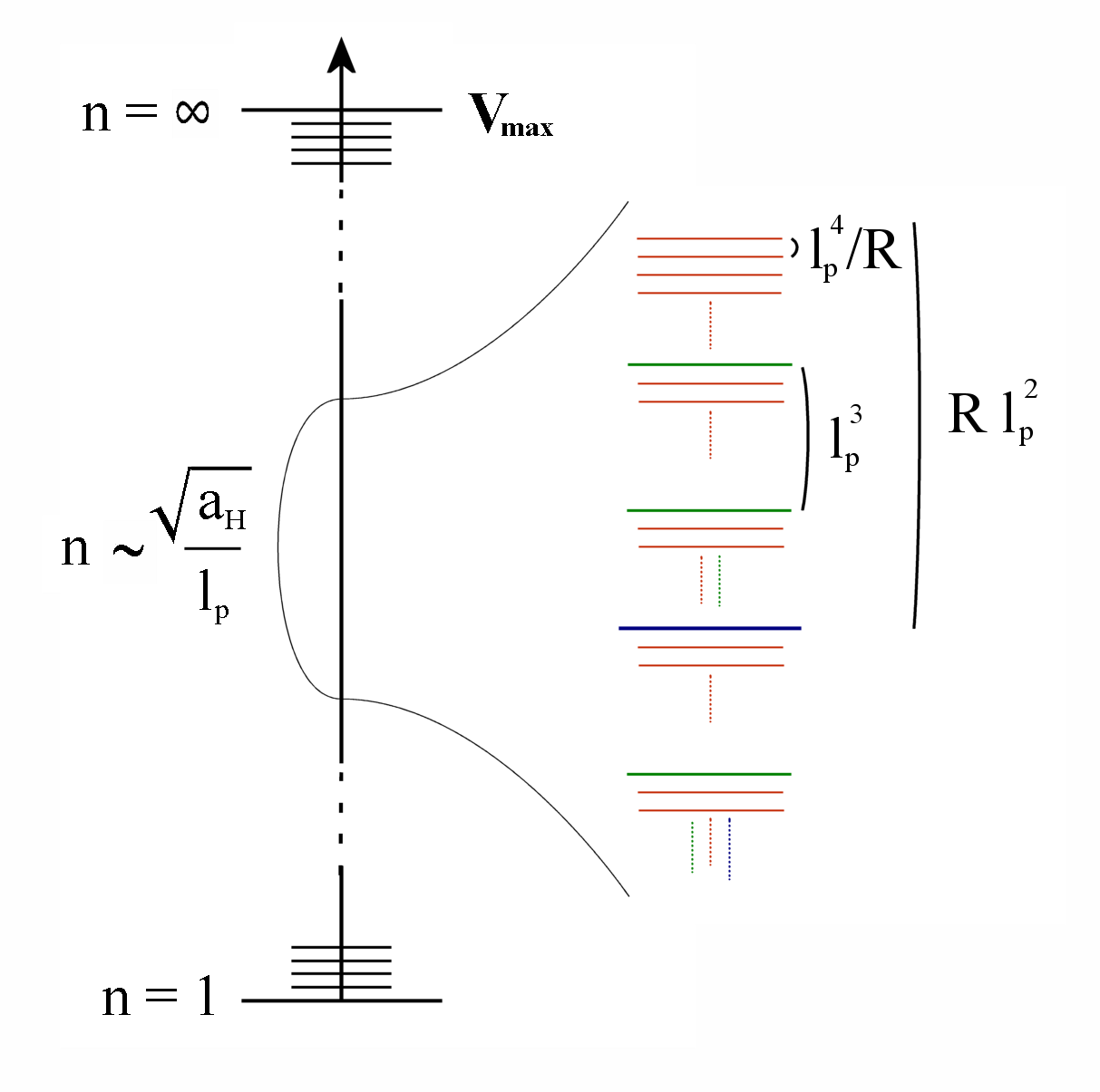
Figure 2: Representation of the spectrum of volume of a black hole in fluid approximation where $n\sim\sqrt{a_{H}}/\ell_{p}$. We represented in the same graph fluctuations of the discrete spins model and those (which are larger) of the continuous representations model. The notation $R$ is for the Schwarzchild radius.

We gather all the quantum fluctuations of the volume together in the figure 2. This graph is instructive because it shows the different scales in the fluctuations even though (40) and (41) concern models where faces are colored with discrete spins whereas (43) concerns models with a continuous representation.

We could also have studied the same type of transformations in the case of an initial configuration where all the representations are not equal. The computations are heavier but we could arrive to the same conclusions: there are three kinds of gap in the volume, the orders of magnitude are the same as the homogeneous case and only the numerical coefficients in the different $\Delta V$ differ.

Note that the black hole spectrum in the deep quantum regime (when $n$ is small) has been studied numerically in spectro1 ; spectro2 for instance.

III.3 Black Hole radiation and Hawking temperature

In this last section, we consider the model of the black hole in the fluid approximation where the puncels are colored with continuous representations. As we have just seen, even when the black hole has a fixed area $a_{H}$, its euclidean volume fluctuates. We suppose that its fluctuations are due to creation/destruction of puncels which rearrange themselves spontaneously according to the transformations $(s,\cdots,s)_{n}\rightarrow(s,\cdots s,s^{\prime},\cdots,s^{\prime})_{n+1}$ described above in subsection (III.2.2). The volume fluctuations are then given by (44) or (43) when all representations rearrange themselves to the same color. We are going to show how the expressions of these fluctuations can be used to propose a model of black hole radiation in the framework of Loop Quantum Gravity.

When the black hole is isolated (interacting with nothing), its area is fixed and nothing could enable us to probe its volume fluctuations. One could mesure these fluctuations only if the black hole interacts with a field whose coupling is sensitive to the volume (in the euclidean picture). In that case, one can access to a measurement of the fluctuations of the volume measuring changes in the field states. When such a field is coupled to the black hole geometry, it excites the internal structure of the quantum black hole and then the typical energy of the field should be closely related to the volume fluctuation of the geometry. We are going to show that it is possible to make such a scenario more precise and we will argue that it could lead us towards a simple fundamental explanation of the Hawking radiation from the point of view of Loop Quantum Gravity.

We start with the expression of the volume fluctuation (43). From a semi-classical point of view, this volume fluctuation can be understood as resulting from a quantum deformation of the horizon of the black hole, and more precisely from a local and quantum deformation of its radius (and the area, hence the total energy is kept fixed). Due to the quantum fluctuations, the black hole is no more spherical and the typical length scale of its mean radius fluctuations (with respect to Schwarzchild radius) is given by

$$\overline{\delta R}\equiv\ell_{v}=\frac{\Delta V_{n}^{(3)}}{a_{H}}\;\sim\;\frac{\ell_{p}^{2}}{\sqrt{a_{H}}}\,.$$ (46)

This length scale is very tiny in the sense that it is much smaller than the Planck length itself. It is supposed to give the mean deformation of the radius on the whole horizon. Because it is small, it can only be explained by a semi-classical configuration of the black hole where the horizon is globally spherical but at some locations there are some defects. These defects have a quantum origine and they slightly modify locally the radius of the black hole. The typical amplitude of these fluctuations is the Planck length $\ell_{p}$ itself which is the smallest (hence the more fundamental) possible length. From the description in terms of puncels, this means that most of the puncels are totally identical but some of them have a defect which locally modify the radius of the horizon with a scale length $\ell_{p}$. More precisely, they should correspond in the fluid approximation to a configuration $(s,\cdots,s,s^{\prime},\cdots,s^{\prime},s^{\prime\prime},\cdots,s^{\prime\prime},\cdots)$ where different “small” paquets of puncels acquire a representation $s^{\prime},s^{\prime\prime},\cdots$ different from $s$.

Let us estimate how many defects are spread on the horizon to reach the mean fluctuation (46). If we denote by $x$ their number, it satisfies the condition

$$\delta R\,\sim\,\frac{x\ell_{p}}{n}\,\sim\,\ell_{v}\,,$$ (47)

This formula is easily interpreted as we compute on the l.h.s. the mean of the radius deformation $\delta R$. As $n\sim\sqrt{a_{H}}/\ell_{p}$, we immediately see that $x$ is necessarily of order $x\sim 1$. As a result, there are few defects (number of order 1) spread of the horizon. This has been illustrated in picture (3). Because of the spherical symmetry, we suppose that the defects form a regular pattern on the horizon. The typical distance between two defects define a wavelength $\lambda$ which characterizes the deformation wave on the horizon. Equivalently, when a field interacts with the black hole, it might be a scattering of the field on these defects, hence the field might excite the “volume” modes when its wavelength scales as $\lambda$. Here $\lambda\sim\sqrt{a_{H}}$ because $x\sim 1$ and the corresponding temperature is given by

$$T\,=\,\frac{h}{\lambda k_{B}}\,\sim\,\frac{h}{GMk_{B}}$$ (48)

where $h$ is the Planck constant, $M$ the mass of the black hole, $G$ the Newton constant and $k_{B}$ the Boltzmann constant. We recover the scaling of the Hawking temperature $T_{H}$

$$T_{H}=\frac{1}{8\pi}\frac{h}{GMk_{B}}\,.$$ (49)

The model is not sufficiently precise to obtain the exact expression of the black hole temperature.

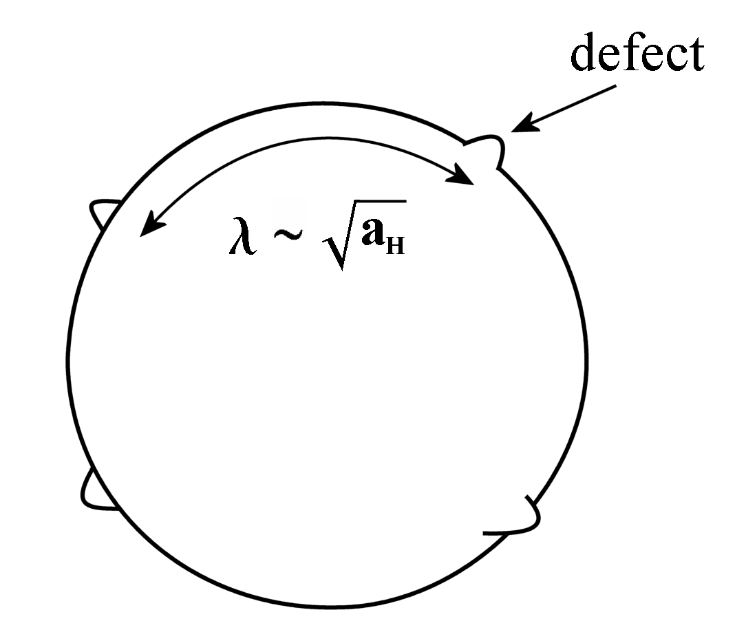
Figure 3: Semi-classical graphical representation of the quantum fluctuation of a black hole. Everything happens as if there were some defects spread on the horizon. These defects form a pattern of typical length $\lambda$. The defects break the spherical symmetry as would do any classical perturbation of the Schwarzchild metric. This length $\lambda$ is supposed to give the typical wavelength of the Hawking radiation of the black hole.

We conclude this Section with one remark. At the semi-classical limit, we have shown that the volume spectrum is linear and then there is a large number of wavelength $\lambda_{p}$ (or equivalently frequencies $\omega_{p}$) labelled by an integer $p$ associated to the different volume gaps and given by $\lambda_{p}=\lambda/p$ or $\omega_{p}=p\,\omega$. In the context of black holes, this reminds us some aspects of quasi-normal modes QNM which, at some classical limit, have been shown to behave in the same way with the difference that they possess also an imaginary part, responsible for the decay of the modes. The real part of quasi-normal modes frequencies scale exactly as the frequencies we found here. Furthermore, quasi-normal modes are also associated to a deformation (from the spherical symmetry) of the black hole horizon. Hence, it would be very interesting to understand whether the analogy between these quantum deformations and quasi-normal modes is deeper.

IV Discussion

In this article, we propose an idea which could help understanding Hawking radiation from the point of view of Loop Quantum Gravity. It is based on some physical arguments and interpretations. But it clearly needs to be studied deeper for us to claim that the scenario we are proposing is indeed realistic. We considered an isolated spherical black hole of fixed area $a_{H}$. Its microstates are intertwiners and they are obviously all eigenstates of the horizon area operator with the same eigenvalue $a_{H}$. Hence, we need another operator (different from the area) to probe the quantum structure of the black hole. We used the euclidean volume operator which indeed raises the degeneracy and allows to probe the internal structure of the microstates. We studied its spectrum in the fluid approximation and we interpreted the volume fluctuations in terms of a quantum deformation of the horizon. We argued that this deformation are described in terms of defects which are regularly spread on the horizon. As the typical length of the defects pattern is $\lambda\sim\sqrt{a_{H}}$, there is a natural temperature associated to the quantum deformation of the black hole which scales as the Hawking temperature. We conclude that Hawking radiation might originate from quantum fluctuations of the horizon.

However, our model is based on many hypothesis and we made used of the euclidean volume to define quantum fluctuations of the horizon. Many points remain to be clarified and we hope to study these aspects in the future. In particular, it would be interesting to have a robust description of the interaction of a field with the black hole in the framework of loop quantum gravity. This could enable us to provide a law energy effective description of the quantum fluctuations and to write a wave equation where the typical length $\lambda$ would appear explicitely. It would also be very instructive to describe the fluid approximation in terms of coherent states, or twisted geometry. We hope to develop these ideas in the future.

References

- (1) J. Bekenstein, Black holes and entropy, Phys. Rev. D 9 2333 (1973).
- (2) S. Hawking, Particle creation by black holes, Comm. Math. Phys. 43 199 (1975).
- (3) C. Rovelli, Black hole entropy from loop quantum gravity, Phys. Rev. Lett. 77 3288 (1996), arXiv: 9603063 [gr-qc].
- (4) A. Ashtekar, C. Beetle and S. Fairhurst, Isolated horizons: A Generalization of black hole mechanics Class.Quant.Grav. 16 (1999) L1-L7, arXiv: 9812065 [gr-qc].
- (5) A. Ashtekar, A. Corichi and K. Krasnov, Isolated horizons: The Classical phase space, Adv.Theor.Math.Phys. 3 (1999) 419-478 , arXiv:9905089 [gr-qc].
- (6) A. Ashtekar, C. Beetle and S. Fairhurst, Mechanics of isolated horizons, Class.Quant.Grav. 17 (2000) 253-298, arXiv: 9907068 [gr-qc].
- (7) A. Ashtekar, S. Fairhurst and B. Krishnan Isolated horizons: Hamiltonian evolution and the first law, Phys.Rev. D62 (2000) 104025, arXiv: 0005083[gr-qc] .
- (8) A. Ashtekar, J. Baez, A. Corichi and K. Krasnov, Quantum geometry and black hole entropy, Phys.Rev.Lett. 80 (1998) 904-907 , arXiv: 9710007 [gr-qc]
- (9) A. Ashtekar, J. C. Baez and K. Krasnov, Quantum geometry of isolated horizons and black hole entropy, Adv.Theor.Math.Phys. 4 (2000) 1-94, arXiv: 0005126 [gr-qc]
- (10) J. Engle, A. Perez and K. Noui, Black hole entropy and SU(2) Chern–Simons theory, Phys. Rev. Lett. 105 031302 (2010), arXiv:0905.3168 [gr-qc].
- (11) J. Engle, K. Noui, A. Perez and D. Pranzetti, Black hole entropy from an SU(2)-invariant formulation of type I isolated horizons, Phys. Rev. D 82 044050 (2010), arXiv:1006.0634 [gr-qc].
- (12) A. Ashtekar, New variables for classical and quantum gravity, Phys. Rev. Lett. 57 2244 (1986).
- (13) J.F. Barbero and A. Perez, Quantum Geometry and Black Holes, arXiv:1501.02963 [gr-qc].
- (14) A. Ghosh and A. Perez, Black hole entropy and isolated horizons thermodynamics, Phys. Rev. Lett. 107 241301 (2011) arXiv: 11071320 [gr-qc].
- (15) E. Frodden, A. Gosh and A. Perez, Quasilocal first law for black hole thermodynamics, Phys. Rev. D 87 121503 (2013), arXiv:1110.4055 [gr-qc].
- (16) E. Bianchi, Entropy of Non-Extremal Black Holes from Loop Gravity, arXiv: 1204.5122 [gr-qc].
- (17) M. Geiller and K. Noui, Near-Horizon Radiation and Self-Dual Loop Quantum Gravity, Europhys. Lett. 105 (2014) 60001, arXiv:1402.4138 [gr-qc].
- (18) J. Ben Achour, A. Mouchet and K. Noui, Analytic continuation of black hole entropy in loop quantum gravity, JHEP 1506 (2015) 145, arXiv:1406.6021 [gr-qc]
- (19) J. Engle, K. Noui, A. Perez and D. Pranzetti, The black hole entropy revisited, JHEP 1105 (2011), arXiv:1103.2723 [gr-qc].
- (20) R. K. Kaul and P. Majumdar, Quantum black hole entropy, Phys. Lett. B 439 (1998) 267 arXiv: 9801080 [gr-qc]
- (21) R. K. Kaul and P. Majumdar, “Logarithmic correction to the Bekenstein-Hawking entropy,” Phys. Rev. Lett. 84 (2000) 5255 arXiv: 0002040 [gr-qc].
- (22) S. Das, R. K. Kaul and P. Majumdar, “A new holographic entropy bound from quantum geometry,” Phys. Rev. D 63 (2001) 044019 arXiv: 0006211 [hep-th/].
- (23) I. Agullo, J. Fernando Barbero, E. F. Borja, J. Diaz-Polo and E. J. S. Villasenor, Detailed black hole state counting in loop quantum gravity, Phys. Rev. D 82 (2010) 084029 arXiv:1101.3660 [gr-qc].
- (24) I. Agullo, G. J. Fernando Barbero, E. F. Borja, J. Diaz-Polo and E. J. S. Villasenor, The combinatorics of the SU(2) black hole entropy in loop quantum gravity, Phys. Rev. D 80 (2009) 084006 arXiv:0906.4529 [gr-qc].
- (25) J. F. Barbero G. and E. J. S. Villasenor, On the computation of black hole entropy in loop quantum gravity, Class. Quant. Grav. 26 (2009) 035017 arXiv:0810.1599 [gr-qc].
- (26) J. F. Barbero G. and E. J. S. Villasenor, Generating functions for black hole entropy in Loop Quantum Gravity, Phys. Rev. D 77 (2008) 121502 arXiv:0804.4784 [gr-qc].
- (27) I. Agullo, J. F. Barbero G., J. Diaz-Polo, E. Fernandez-Borja and E. J. S. Villasenor, Black hole state counting in LQG: A number theoretical approach, Phys. Rev. Lett. 100 (2008) 211301 arXiv:0802.4077 [gr-qc].
- (28) K. A. Meissner, Black hole entropy in loop quantum gravity, Class. Quant. Grav. 21 5245 (2004), arXiv: 0407052 [gr-qc].
- (29) E. R. Livine and D. R. Terno, Entropy in the Classical and Quantum Polymer Black Hole Models, Class.Quant.Grav. 29 (2012) 224012, arXiv:1205.5733 [gr-qc]
- (30) E. Bianchi, Black Hole Entropy, Loop Gravity, and Polymer Physics, Class.Quant.Grav. 28 (2011) 114006, arXiv:1011.5628 [gr-qc]
- (31) E. Frodden, A. Perez, D. Pranzetti and C. Ro ken, Modelling black holes with angular momentum in loop quantum gravity, Gen. Rel. Grav. 46 (2014) 1828. arXiv:1011.2961 [gr-qc]
- (32) J. Ben Achour, K. Noui and A. Perez, Analytic continuation of the rotating black hole state counting, JHEP 1608 (2016) 149, arXiv:1607.02380 [gr-qc].
- (33) A. Ghosh, K. Noui and A. Perez, Statistics, holography, and black hole entropy in loop quantum gravity, Phys. Rev. D (2014), arXiv:1309.4563 [gr-qc].
- (34) E. Frodden, M. Geiller, K. Noui and A. Perez, Black hole entropy from complex Ashtekar variables, accepted to Eur. Phys. Lett. (2014), arXiv:1212.4060 [gr-qc].
- (35) J. Ben Achour and K. Noui, Analytic continuation of real Loop Quantum Gravity : Lessons from black hole thermodynamics, PoS FFP14 (2015) 158, arXiv:1501.05523 [gr-qc]
- (36) J. Ben Achour, Towards self dual Loop Quantum Gravity, (2015), arXiv:1511.07332 [gr-qc]
- (37) E. Frodden, M. Geiller, K. Noui and A. Perez, Statistical entropy of a BTZ black hole from loop quantum gravity, JHEP 5 139 (2013), arXiv:1212.4473 [gr-qc].
- (38) J. Ben Achour, M. Geiller, K. Noui and C. Yu, Testing the role of the Barbero–Immirzi parameter and the choice of connection in loop quantum gravity, (2013), arXiv:1306.3241 [gr-qc].
- (39) J. Ben Achour, M. Geiller, K. Noui and C. Yu, Spectra of geometric operators in three-dimensional LQG: From discrete to continuous, accepted to Phys. Rev. D (2013), arXiv:1306.3246 [gr-qc].
- (40) D. Pranzetti, Geometric temperature and entropy of quantum isolated horizons, Phys.Rev. D89 (2014) no.10, 104046, arXiv:1305.6714 [gr-qc]
- (41) D. Pranzetti, H. Sahlmann, Horizon entropy with loop quantum gravity methods, Phys.Lett. B746 (2015) 209-216, arXiv:1412.7435 [gr-qc]
- (42) D. Pranzetti, Black hole entropy from KMS-states of quantum isolated horizons, arXiv:1305.6714 [gr-qc].
- (43) A. Perez and D. Pranzetti, Static isolated horizons: SU(2) invariant phase space, quantization, and black hole entropy, Entropy 13 (2011) 744-777, arXiv: arXiv:1011.2961 [gr-qc]
- (44) Y. Neiman, The imaginary part of the gravity action and black hole entropy, JHEP 71 (2013), arXiv:1212.2922 [gr-qc].
- (45) Y. Neiman, The imaginary part of the gravity action at asymptotic boundaries and horizons, Phys. Rev. D88 024037 (2013), arXiv:1305.2207 [gr-qc].
- (46) N. Bodendorfer and Y. Neiman, Imaginary action, spinfoam asymptotics and the ‘transplanckian’ regime of loop quantum gravity, Class. Quant. Grav. 30 195018 (2013), arXiv:1303.4752 [gr-qc].
- (47) M. Han, Black hole entropy in loop quantum gravity, analytic continuation, and dual holography, (2014), arXiv:1402.2084 [gr-qc].
- (48) J. Brunnemann and T. Thiemann, Simplication of the spectral analysis of the volume operator in loop quantum gravity, Class. Quant. Grav. 23, 1289, 2006, arXiv:gr-qc/0405060.
- (49) A. Barrau, T. Cailleteau, X. Cao, J. Diaz-Polo, and J. Grain, Probing Loop Quantum Gravity with Evaporating Black Holes, Phys.Rev.Lett., 107:251301, 2011.
- (50) A. Barrau, X. Cao, K. Noui and A. Perez, Black Hole spectroscopy from Loop Quantum Gravity models, Phys. Rev. D92, 124046, 2015, arXiv:1504.05352 [gr-qc].
- (51) K. Kokkotas and B. Schmidt, Quasi-Normal modes of stars and black holes, LivingRev.Rel.2:2 (1999), arXiv:gr-qc/9909058.