Non-parabolic diffusion problems in one space dimension

Abstract.

We study some non-parabolic diffusion problems in one-space dimension, where the diffusion flux exhibits forward and backward nature of the Perona-Malik, Höllig or non-Fourier type. Classical weak solutions to such problems are constructed in a way to capture some expected and unexpected properties, including anomalous asymptotic behaviors and energy dissipation or allocation. Specific properties of solutions will depend on the type of the diffusion flux, but the primary method of our study relies on reformulating diffusion equations involved as an inhomogeneous partial differential inclusion and on constructing solutions from the differential inclusion by a combination of the convex integration and Baire’s category methods. In doing so, we introduce the appropriate notion of subsolutions of the partial differential inclusion and their transition gauge, which plays a pivotal role in dealing with some specific features of the constructed weak solutions.

1. Introduction

In this paper, we study the initial-boundary value problem of quasilinear diffusion equations in one space dimension:

(1.1) $$\left\{\begin{array}[]{ll}u_{t}=(\sigma(u_{x}))_{x}&\mbox{in $\Omega\times(0,T)$,}\\ u=u_{0}&\mbox{on $\Omega\times\{t=0\}$,}\\ \sigma(u_{x})=0&\mbox{on $\partial\Omega\times(0,T)$.}\end{array}\right.$$

Here, $\Omega=(0,L)\subset\mathbb{R}$ with $L>0$, $T\in(0,\infty]$ is given, $\sigma=\sigma(s)$ is the diffusion flux function on $\mathbb{R}$, $u_{0}=u_{0}(x)$ is a given initial function on $\Omega,$ and $u=u(x,t)$ is a solution to the problem.

The diffusion equation in (1.1) becomes a formal gradient flow of the energy functional $\mathcal{E}$ defined by

$$\mathcal{E}(p)=\int_{0}^{L}W(p_{x})\,dx,$$

where $W=W(s)$ is an antiderivative of the diffusion flux $\sigma.$ When the diffusion flux $\sigma$ is smooth with $\sigma^{\prime}>0$ in $\mathbb{R}$, problem (1.1) is parabolic so that by the classical parabolic theory [15, 16], it possesses a unique global classical solution that belongs to the parabolic Hölder space $C^{2+\alpha,1+\frac{\alpha}{2}}(\bar{\Omega}\times[0,\tau])$ with $\alpha\in(0,1)$ for all $0<\tau<\infty$ if the initial datum $u_{0}$ is in $C^{2+\alpha}(\bar{\Omega})$ and satisfies the compatibility condition (1.3).

However, in many applications and models of diffusion process, the diffusion fluxes $\sigma$ are not increasing on $\mathbb{R}$, as have been studied in phase transition problems in thermodynamics [5, 6], mathematical models of stratified turbulent flows [1], ecological models of population dynamics [17, 18], image processing [19], and gradient flows associated with nonconvex energy functionals [20]. Therefore, in such cases, problem (1.1) becomes non-parabolic, and the standard methods of parabolic theory are not applicable to study existence and uniqueness or non-uniqueness of solutions for arbitrary initial data $u_{0}\in C^{2+\alpha}(\bar{\Omega})$ satisfying the compatibility condition (1.3).

For a general flux function $\sigma$, the equation in (1.1) is in divergence form and hence a natural generalized solution to problem (1.1) can be defined in the usual variational sense. In the following, we use $W^{1,\infty}_{loc}(\Omega\times[0,T))$ to denote the set of functions $u\in C(\bar{\Omega}\times[0,T))$ such that $u\in W^{1,\infty}(\Omega\times(0,\tau))$ for all $\tau\in(0,T)$. A function $u\in W^{1,\infty}_{loc}(\Omega\times[0,T))$ is called a weak solution to (1.1) provided that equality

(1.2) $$\int_{0}^{L}\big{(}u(x,\tau)\zeta(x,\tau)-u_{0}(x)\zeta(x,0)\big{)}\,dx=\int_{0}^{\tau}\int_{0}^{L}\big{(}u\zeta_{t}-\sigma(u_{x})\zeta_{x}\big{)}\,dxdt$$

holds for each $\zeta\in C^{\infty}(\bar{\Omega}\times[0,T))$ and each $\tau\in[0,T).$ In case of $T=\infty$, such a solution $u$ is said to be global. Upon taking $\zeta\equiv 1$ in (1.2), it is immediate that every weak solution $u$ to (1.1) fulfills the conservation of total mass at all times:

$$\int_{0}^{L}u(x,t)\,dx=\int_{0}^{L}u_{0}(x)\,dx\;\;\forall t\in[0,T).$$

In this paper, we focus on the three main types of non-increasing diffusion flux functions $\sigma$: the Höllig type in [5], the Perona-Malik type in [19], and the non-Fourier type with double-well potential $W(s)$. Therefore, the diffusion fluxes $\sigma\in C(\mathbb{R})$ under consideration have potential $\mathbb{R}\ni s\mapsto\int_{0}^{s}\sigma(l)\,dl$ that attains an absolute minimum; throughout the paper, we let $W\in C^{1}(\mathbb{R})$ denote the antiderivative of $\sigma$ whose absolute minimum value is $0$. The initial datum $u_{0}$ will always be in the class $C^{2+\alpha}(\bar{\Omega})$ for a fixed $0<\alpha<1$ and satisfy the compatibility condition

(1.3) $$u_{0}^{\prime}(0)=u_{0}^{\prime}(L)=0.$$

We remark that for diffusion equations of the Perona-Malik type and certain specific initial data $u_{0}$ with $u_{0}^{\prime}$ exhibiting backward phases, the classical solutions were constructed in the works [3, 4]. For such equations with general initial data, it has been known that the Neumann problem may not have a classical solution [7, 8].

The main purpose of this paper is to construct weak solutions to problem (1.1) with diffusion fluxes $\sigma$ of the three types above that capture some expected and unexpected properties, including anomalous asymptotic behaviors and energy dissipation or allocation. Our construction relies on the important technique by Zhang [21, 22] of reformulating diffusion equations involved as an inhomogeneous partial differential inclusion; such a technique has been recently generalized by the authors to handle more general problems, including the high-dimensional ones, through a combination of the convex integration and Baire’s category methods; see [11, 12, 13, 14].

However, to construct weak solutions with certain specific features, as in [14], we need to introduce appropriate subsolutions of the associated partial differential inclusion and their transition gauge and to iterate some constructions while controlling the gauge. The controllable gauge, combined with the result on a one-dimensional parabolic problem [10], will enable us to iterate the constructions and eventually lead us to extract energy dissipation for the Perona-Malik type diffusions and energy allocation for the non-Fourier type diffusions as well as the blow-up or concentration of the spatial derivative of weak solutions.

Our main results will be introduced in Section 2, where we fix the hypothesis on the diffusion flux $\sigma$ of the Höllig, Peorna-Malik and non-Fourier types respectively, state the main results corresponding to each type, and discuss some interesting features of those results.

Other than the statements of the main results, the rest of the paper is organized as follows. In Section 3, we prepare all the essential ingredients needed to prove our main results, some of which may be of independent interest; in this section (see Subsection 3.2), we also provide the easy proofs for Theorems 2.1 and 2.3. In Section 4, the proof of Theorem 2.2 is given to obtain global weak solutions to (1.1) that are smooth after a finite time when $\sigma$ is of the Höllig type. For the same type of solutions to (1.1) when $\sigma$ is of the Perona-Malik type, the proof of Theorems 2.4 and 2.5 is given in Section 5. Section 6 is devoted to the proof of Theorem 2.6 on the weak solutions to (1.1) with anomalous blow-up and vanishing energy when $\sigma$ is of the Perona-Malik type. In Section 7, global weak solutions to (1.1) with energy allocation are constructed when $\sigma$ is of the non-Fourier type to prove Theorem 2.7. In the last part of the paper, Section 8, the key density lemma, Lemma 3.5, is proved.

2. Statement of main results

We begin this section by fixing some notation. We denote by $\mathbb{M}^{m\times n}$ the space of $m\times n$ real matrices. We write $\Omega_{\tau}=\Omega\times(0,\tau)$ for each $\tau\in(0,\infty]$ and $\|\cdot\|_{\infty}=\|\cdot\|_{L^{\infty}(\Omega)}$. We let $\bar{u}_{0}$ denote the mean value of the initial datum $u_{0}$ over $\Omega$; that is, $\bar{u}_{0}=\frac{1}{L}\int_{0}^{L}u_{0}(x)\,dx\in\mathbb{R}.$ We also write

$$M_{0}=\max_{\bar{\Omega}}u_{0}^{\prime}\;\;\mbox{and}\;\;m_{0}=\min_{\bar{\Omega}}u_{0}^{\prime};$$

so $m_{0}\leq 0\leq M_{0}$. For a bounded open set $U\subset\mathbb{R}^{n}$ with its coordinates $(z_{1},\cdots,z_{n})$, $W^{1,\infty}(U)$ denotes the space of functions $f\in L^{\infty}(U)$ with $f_{z_{i}}\in L^{\infty}(U)$ $(i=1,\cdots,n)$ and norm $\|f\|_{W^{1,\infty}(U)}:=\|f\|_{L^{\infty}(U)}+\sum_{i=1}^{n}\|f_{z_{i}}\|_{L^{\infty}(U)}$, and $W^{1,\infty}_{0}(U)$ consists of the functions $f\in W^{1,\infty}(U)$ with zero trace on $\partial U.$ For integers $k,l\geq 0$ with $2l\leq k$, we denote by $C^{k,l}(\bar{\Omega}_{\tau})$, with $0<\tau\leq\infty$, the space of functions $u\in C(\bar{\Omega}_{\tau})$ such that $D^{i}_{x}D^{j}_{t}u\in C(\bar{\Omega}_{\tau})$ for all integers $0\leq i\leq k$ and $0\leq j\leq l$ with $i+2j\leq k$. For other function spaces, we mainly follow the notations in the book [15], with one exception that the letter $C$ is used instead of $H$ regarding suitable parabolic Hölder spaces.

2.1. Höllig type equations

In this subsection, we consider a class of flux functions $\sigma$ that includes piecewise linear ones, studied by Höllig [5], and present the results on large time behaviors of global weak or classical solutions to problem (1.1).

To be precise, we impose the following conditions on the flux function $\sigma\in C(\mathbb{R})$ (see Figure 1): there exist three numbers $\bar{s}_{2}>s_{2}>s_{1}>0$ such that

• $\sigma\in C^{3}((-\infty,s_{1})\cup(s_{2},\infty)),$

• $\sigma>0$ on $(s_{1},s_{2})$, $\sigma^{\prime}>0$ in $(-\infty,s_{1})\cup(s_{2},\infty)$, and

• $\sigma(\bar{s}_{2})=\sigma(s_{1})>\sigma(s_{2})>\sigma(0)=0$.

Let $\bar{s}_{1}\in(0,s_{1})$ denote the unique number with $\sigma(\bar{s}_{1})=\sigma(s_{2})$. For each $r\in(\sigma(s_{2}),\sigma(s_{1}))$, let $s^{+}_{r}\in(s_{2},\bar{s}_{2})$ and $s^{-}_{r}\in(\bar{s}_{1},s_{1})$ be the unique numbers such that $\sigma(s^{\pm}_{r})=r$.

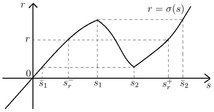
Figure 1. Diffusion flux $\sigma(s)$ of the Höllig type

2.1.1. Global classical solution

The following is a result on the global classical solution $u$ to problem (1.1) when the maximum $M_{0}$ of $u_{0}^{\prime}$ on $\bar{\Omega}$ is less than the threshold $s_{1}$.

Theorem 2.1 (Global classical solution).

Assume

$$M_{0}<s_{1}.$$

Then there exists a unique global solution $u\in C^{2,1}(\bar{\Omega}_{\infty})$ to problem (1.1) satisfying the following properties:

• for each $\tau>0$, $u\in C^{2+\alpha,1+\alpha/2}(\bar{\Omega}_{\tau})$,

• for all $t_{2}>t_{1}\geq 0,$

  $$\min_{\bar{\Omega}}u(\cdot,t_{1})\leq\min_{\bar{\Omega}}u(\cdot,t_{2})\leq\bar{u}_{0}\leq\max_{\bar{\Omega}}u(\cdot,t_{2})\leq\max_{\bar{\Omega}}u(\cdot,t_{1}),$$

• for all $t_{2}>t_{1}\geq 0,$

  $$\min_{\bar{\Omega}}u_{x}(\cdot,t_{1})\leq\min_{\bar{\Omega}}u_{x}(\cdot,t_{2})\leq 0\leq\max_{\bar{\Omega}}u_{x}(\cdot,t_{2})\leq\max_{\bar{\Omega}}u_{x}(\cdot,t_{1}),$$

• $\|u(\cdot,t)-\bar{u}_{0}\|_{W^{1,\infty}(\Omega)}\leq Ce^{-\gamma t}$ for all $t\geq 0$, where $C>0$ and $\gamma>0$ are some constants depending only on $u_{0}$, $\sigma$ and $L$.

2.1.2. Global weak solutions that are smooth after a finite time

When $M_{0}$ is greater than the threshold $\bar{s}_{1}$, we can get infinitely many global weak solutions $u$ to problem (1.1) that become identical and smooth after a finite time.

Theorem 2.2 (Eventual smoothing).

Assume

$$M_{0}>\bar{s}_{1}$$

so that $\bar{s}_{1}<u_{0}^{\prime}(x_{0})<\bar{s}_{2}$ for some $x_{0}\in\Omega.$ Let $\sigma(s_{2})<r_{1}<r_{2}<\sigma(s_{1})$ be any two numbers such that $s^{-}_{r_{1}}<u_{0}^{\prime}(x_{0})<s^{+}_{r_{2}}$. Then there exists a function $u^{*}\in C^{2,1}(\bar{\Omega}_{\infty})$ such that for each $\epsilon>0$, there are infinitely many global weak solutions $u$ to problem (1.1) satisfying the following properties: letting

$$\begin{split}Q_{1}&=\big{\{}(x,t)\in\Omega_{\infty}\,|\,s^{-}_{r_{1}}<u^{*}_{x}(x,t)<s^{+}_{r_{2}}\big{\}},\\ Q_{2}&=\big{\{}(x,t)\in\Omega_{\infty}\,|\,u^{*}_{x}(x,t)>s^{+}_{r_{2}}\big{\}},\\ F^{+}&=\big{\{}(x,t)\in\Omega_{\infty}\,|\,u^{*}_{x}(x,t)=s^{+}_{r_{2}}\big{\}},\\ F^{-}&=\big{\{}(x,t)\in\Omega_{\infty}\,|\,u^{*}_{x}(x,t)=s^{-}_{r_{1}}\big{\}},\end{split}$$

we have

• $u=u^{*}$ in $\bar{\Omega}_{\infty}\setminus Q_{1}$, $\|u-u^{*}\|_{L^{\infty}(Q_{1})}<\epsilon$, $\|u_{t}-u_{t}^{*}\|_{L^{\infty}(Q_{1})}<\epsilon$,

• $u_{x}\in[s^{-}_{r_{1}},s^{-}_{r_{2}}]\cup[s^{+}_{r_{1}},s^{+}_{r_{2}}]$ a.e. in $Q_{1}$, $u_{x}=s^{+}_{r_{2}}$ a.e. in $F^{+}$, $u_{x}=s^{-}_{r_{1}}$ a.e. in $F^{-}$,

• $\big{|}\big{\{}(x,t)\in Q_{1}\,|\,u_{x}(x,t)\in[s^{\pm}_{r_{1}},s^{\pm}_{r_{2}}]\big{\}}\big{|}>0$,

• $Q_{1}\cup Q_{2}\cup F^{+}\cup F^{-}$ is a bounded set whose closure is contained in $\Omega\times[0,\infty)$,

• $0\leq\underset{(x,t)\in Q_{2}}{\sup}t<\underset{(x,t)\in Q_{1}}{\sup}t<\infty$,

• for each $\tau>0$, $u^{*}\in C^{2+\alpha,1+\alpha/2}(\bar{\Omega}_{\tau})$,

• for all $t_{2}>t_{1}\geq 0,$

  $$\min_{\bar{\Omega}}u^{*}(\cdot,t_{1})\leq\min_{\bar{\Omega}}u^{*}(\cdot,t_{2})\leq\bar{u}_{0}\leq\max_{\bar{\Omega}}u^{*}(\cdot,t_{2})\leq\max_{\bar{\Omega}}u^{*}(\cdot,t_{1}),$$

• for all $t_{2}>t_{1}\geq 0,$

  $$\min_{\bar{\Omega}}u^{*}_{x}(\cdot,t_{1})\leq\min_{\bar{\Omega}}u^{*}_{x}(\cdot,t_{2})\leq 0\leq\max_{\bar{\Omega}}u^{*}_{x}(\cdot,t_{2})\leq\max_{\bar{\Omega}}u^{*}_{x}(\cdot,t_{1}),$$

• $\|u^{*}(\cdot,t)-\bar{u}_{0}\|_{W^{1,\infty}(\Omega)}\leq Ce^{-\gamma t}$ for all $t\geq 0$, where $C>0$ and $\gamma>0$ are some constants depending only on $u_{0}$, $\sigma$, $r_{1}$, $r_{2}$ and $L$.

2.1.3. Remarks

Depending on the maximum value $M_{0}$ of $u_{0}^{\prime}$ on $\bar{\Omega}$, we may have several possible scenarios on the existence of classical solutions to problem (1.1).

• (Coexistence) When $\bar{s}_{1}<M_{0}<s_{1}$, from Theorems 2.1 and 2.2, we have the coexistence of a unique global classical solution and infinitely many global weak (but eventually classical) solutions to problem (1.1). This pathological feature of the existence theory seems to arise from forward and backward nature of the diffusion flux $\sigma$ of the Höllig type although, in this case, the classical solution may be the most natural representative.

• (Critical case) The case $M_{0}=s_{1}$ is rather subtle. If, in addition, $\sigma\in C^{3}((-\infty,s_{1}])$ and $\sigma^{\prime}(s_{1})>0$, we can get a unique global classical solution $u$ to problem (1.1) as in Theorem 2.1. On the other hand, if, in addition, $\sigma\in C^{3}((-\infty,s_{1}])$ and $\sigma^{\prime}(s_{1})=0$, one may have to rely on the degenerate parabolic theory, which we will not address here. However, no matter what we assume for the diffusion flux $\sigma$ at $s=s_{1}$, by Theorem 2.2, we still have infinitely many global weak solutions to (1.1) that are smooth after a finite time.

• (Nonexistence of classical solution) If $M_{0}>s_{1}$, there can be no classical solution to problem (1.1) at all for a large class of initial data $u_{0}$. For example, let us assume in addition that $\sigma\in C^{\infty}(\mathbb{R})$ and that $\sigma^{\prime}<0$ in $(s_{1},s_{2})$. Since $M_{0}>s_{1}$ and $u_{0}^{\prime}=0$ on $\partial\Omega$, there is a nonempty open interval $I\subset\Omega$ on which $u_{0}^{\prime}$ falls into the backward regime $(s_{1},s_{2})$. So one can readily check as in [8] that there is no classical solution (not even a local $C^{1}$ solution) to (1.1) unless $u_{0}$ were infinitely differentiable from the start. Even in the case that $u_{0}$ is infinitely differentiable, it is not at all obvious if there is a local or global classical solution to (1.1); in this regard, see [3, 4]. Regardless of such possible nonexistence of a classical solution, Theorem 2.2 still guarantees the existence of global weak solutions to (1.1) that are smooth after a finite time.

• (Breakdown of uniqueness) From the first discussion above, one may expect that if $M_{0}\leq\bar{s}_{1}$, there exists a unique global weak (and necessarily classical) solution to problem (1.1). Regarding this, we define the number

  $$s_{cr}=\sup\left\{s\geq 0\,\bigg{|}\,\begin{array}[]{l}\mbox{$\forall u_{0}\in C^{2+\alpha}(\bar{\Omega})$ with $u_{0}^{\prime}=0$ on $\partial\Omega$}\\ \mbox{and $\max_{\bar{\Omega}}u_{0}^{\prime}\leq s,$ there exists a unique }\\ \mbox{global weak solution to (\ref{main-ibP})}\end{array}\right\}.$$

  From Theorem 2.2, it is easy to see that $s_{cr}\leq\bar{s}_{1}$. Following [6, 13], one can also check that $s_{cr}>0$. Nonetheless, it seems not simple to answer if $s_{cr}=\bar{s}_{1}$ or not.

2.2. Perona-Malik type equations

Here, we consider a class of flux functions $\sigma$ that contains the Perona-Malik functions in [19]:

$$\sigma(s)=\frac{s}{1+s^{2}}\;\;\mbox{and}\;\;\sigma(s)=se^{-s^{2}/2}.$$

Specifically, we assume the following conditions on the flux function $\sigma\in C(\mathbb{R})$ (see Figure 2): there exist two numbers $s_{1}<0<s_{2}$ such that

• $\sigma\in C^{3}(s_{1},s_{2}),$

• $\sigma^{\prime}>0$ in $(s_{1},s_{2})$, $\sigma(0)=0$,

• $\sigma$ is strictly decreasing on $(-\infty,s_{1}]\cup[s_{2},\infty)$, and

• $\underset{s\to\pm\infty}{\lim}\sigma(s)=0.$

For each $r\in(0,\sigma(s_{2}))$, let $s^{+}_{r}\in(s_{2},\infty)$ and $s^{-}_{r}\in(0,s_{2})$ denote the unique numbers with $\sigma(s^{\pm}_{r})=r$. Similarly, for each $r\in(\sigma(s_{1}),0)$, let $s^{+}_{r}\in(s_{1},0)$ and $s^{-}_{r}\in(-\infty,s_{1})$ be the unique numbers such that $\sigma(s^{\pm}_{r})=r$.

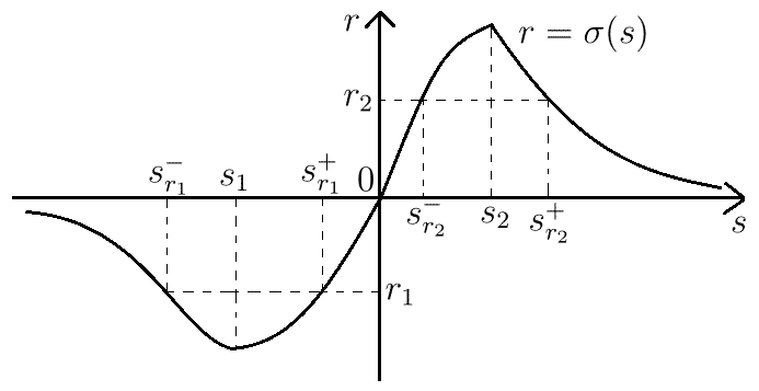
Figure 2. Diffusion flux $\sigma(s)$ of the Perona-Malik type

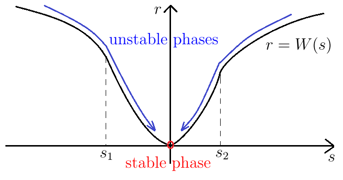
Figure 3. Potential function $W(s)$ of the Perona-Malik type

2.2.1. Global classical solution

Since the flux function $\sigma(s)$ has a positive derivative for values $s$ near $0$, similarly as in Theorem 2.1, we have a global classical solution $u$ to problem (1.1) for initial data $u_{0}$ with sufficiently small $M_{0}$ and $m_{0}$.

Theorem 2.3 (Global classical solution).

Assume

$$s_{1}<m_{0}\leq 0\leq M_{0}<s_{2}.$$

Then there exists a unique global solution $u\in C^{2,1}(\bar{\Omega}_{\infty})$ to problem (1.1) satisfying the following properties:

• for each $\tau>0$, $u\in C^{2+\alpha,1+\alpha/2}(\bar{\Omega}_{\tau})$,

• for all $t_{2}>t_{1}\geq 0,$

  $$\min_{\bar{\Omega}}u(\cdot,t_{1})\leq\min_{\bar{\Omega}}u(\cdot,t_{2})\leq\bar{u}_{0}\leq\max_{\bar{\Omega}}u(\cdot,t_{2})\leq\max_{\bar{\Omega}}u(\cdot,t_{1}),$$

• for all $t_{2}>t_{1}\geq 0,$

  $$\min_{\bar{\Omega}}u_{x}(\cdot,t_{1})\leq\min_{\bar{\Omega}}u_{x}(\cdot,t_{2})\leq 0\leq\max_{\bar{\Omega}}u_{x}(\cdot,t_{2})\leq\max_{\bar{\Omega}}u_{x}(\cdot,t_{1}),$$

• $\|u(\cdot,t)-\bar{u}_{0}\|_{W^{1,\infty}(\Omega)}\leq Ce^{-\gamma t}$ for all $t\geq 0$, where $C>0$ and $\gamma>0$ are some constants depending only on $u_{0}$, $\sigma$ and $L$.

2.2.2. Global weak solutions that are smooth after a finite time

For any nonconstant smooth initial datum $u_{0}$, we have multiple global weak solutions $u$ to problem (1.1) that are classical after a finite time as in the following theorems. Note that $\{0\}\subsetneq[m_{0},M_{0}]$ when $u_{0}$ is nonconstant.

The first one deals with the case that none of $M_{0}$ and $m_{0}$ are equal to $0$.

Theorem 2.4 (Eventual smoothing: Case 1).

Assume

$$m_{0}<0<M_{0}.$$

Let $\sigma(s_{1})<r_{1}<0<r_{2}<\sigma(s_{2})$ be any two numbers such that

$$s^{-}_{r_{1}}<m_{0}<s^{+}_{r_{1}}<0<s^{-}_{r_{2}}<M_{0}<s^{+}_{r_{2}},$$

and let $r_{1}^{\prime}\in(\sigma(s_{1}),r_{1})$, $r_{2}^{\prime}\in(r_{2},\sigma(s_{2}))$ be any two numbers. Then there exists a function $u^{*}\in C^{2,1}(\bar{\Omega}_{\infty})$ such that for each $\epsilon>0$, there are infinitely many global weak solutions $u$ to problem (1.1) satisfying the following properties: letting

$$\begin{split}Q_{1}&=\big{\{}(x,t)\in\Omega_{\infty}\,|\,s^{-}_{r_{1}}<u^{*}_{x}(x,t)<s^{+}_{r_{1}}\big{\}},\\ Q_{2}&=\big{\{}(x,t)\in\Omega_{\infty}\,|\,s^{-}_{r_{2}}<u^{*}_{x}(x,t)<s^{+}_{r_{2}}\big{\}},\\ F_{1}&=\big{\{}(x,t)\in\Omega_{\infty}\,|\,u^{*}_{x}(x,t)=s^{+}_{r_{1}}\big{\}},\\ F_{2}&=\big{\{}(x,t)\in\Omega_{\infty}\,|\,u^{*}_{x}(x,t)=s^{-}_{r_{2}}\big{\}},\end{split}$$

we have

• $u=u^{*}$ in $\bar{\Omega}_{\infty}\setminus(Q_{1}\cup Q_{2})$, $\|u-u^{*}\|_{L^{\infty}(Q_{1}\cup Q_{2})}<\epsilon$, $\|u_{t}-u_{t}^{*}\|_{L^{\infty}(Q_{1}\cup Q_{2})}<\epsilon$,

• $\left\{\begin{array}[]{l}\mbox{$u_{x}\in[s^{-}_{r_{1}},s^{-}_{r_{1}^{\prime}}]\cup[s^{+}_{r_{1}^{\prime}},s^{+}_{r_{1}}]$ a.e. in $Q_{1}$, $u_{x}=s^{+}_{r_{1}}$ a.e. in $F_{1}$,}\\ \mbox{$u_{x}\in[s^{-}_{r_{2}},s^{-}_{r_{2}^{\prime}}]\cup[s^{+}_{r_{2}^{\prime}},s^{+}_{r_{2}}]$ a.e. in $Q_{2}$, $u_{x}=s^{-}_{r_{2}}$ a.e. in $F_{2}$,}\end{array}\right.$

• $\left\{\begin{array}[]{l}\mbox{$\big{|}\big{\{}(x,t)\in Q_{1}\,|\,u_{x}(x,t)\in[s^{-}_{r_{1}},s^{-}_{r_{1}^{\prime}}]\big{\}}\big{|}>0$,}\\ \mbox{$\big{|}\big{\{}(x,t)\in Q_{1}\,|\,u_{x}(x,t)\in[s^{+}_{r_{1}^{\prime}},s^{+}_{r_{1}}]\big{\}}\big{|}>0$,}\\ \mbox{$\big{|}\big{\{}(x,t)\in Q_{2}\,|\,u_{x}(x,t)\in[s^{-}_{r_{2}},s^{-}_{r_{2}^{\prime}}]\big{\}}\big{|}>0$,}\\ \mbox{$\big{|}\big{\{}(x,t)\in Q_{2}\,|\,u_{x}(x,t)\in[s^{+}_{r_{2}^{\prime}},s^{+}_{r_{2}}]\big{\}}\big{|}>0$,}\end{array}\right.$

• $Q_{1}\cup Q_{2}\cup F_{1}\cup F_{2}$ is a bounded set whose closure is contained in $\Omega\times[0,\infty)$,

• for each $\tau>0$, $u^{*}\in C^{2+\alpha,1+\alpha/2}(\bar{\Omega}_{\tau})$,

• for all $t_{2}>t_{1}\geq 0,$

  $$\min_{\bar{\Omega}}u^{*}(\cdot,t_{1})\leq\min_{\bar{\Omega}}u^{*}(\cdot,t_{2})\leq\bar{u}_{0}\leq\max_{\bar{\Omega}}u^{*}(\cdot,t_{2})\leq\max_{\bar{\Omega}}u^{*}(\cdot,t_{1}),$$

• for all $t_{2}>t_{1}\geq 0,$

  $$\min_{\bar{\Omega}}u^{*}_{x}(\cdot,t_{1})\leq\min_{\bar{\Omega}}u^{*}_{x}(\cdot,t_{2})\leq 0\leq\max_{\bar{\Omega}}u^{*}_{x}(\cdot,t_{2})\leq\max_{\bar{\Omega}}u^{*}_{x}(\cdot,t_{1}),$$

• $\|u^{*}(\cdot,t)-\bar{u}_{0}\|_{W^{1,\infty}(\Omega)}\leq Ce^{-\gamma t}$ for all $t\geq 0$, where $C>0$ and $\gamma>0$ are some constants depending only on $u_{0}$, $\sigma$, $r_{1}$, $r_{1}^{\prime}$, $r_{2}$, $r_{2}^{\prime}$ and $L$.

Unlike Case 1 above, when $m_{0}=0$, our global weak solutions $u$ to problem (1.1) have no negative spatial derivative at all times as follows.

Theorem 2.5 (Eventual smoothing: Case 2).

Assume

$$0=m_{0}<M_{0}.$$

Let $0<r_{0}<\sigma(s_{2})$ be any number such that

$$s^{-}_{r_{0}}<M_{0}<s^{+}_{r_{0}},$$

and let $r_{0}^{\prime}\in(r_{0},\sigma(s_{2}))$ be any number. Then there exists a function $u^{*}\in C^{2,1}(\bar{\Omega}_{\infty})$ such that for each $\epsilon>0$, there are infinitely many global weak solutions $u$ to problem (1.1) satisfying the following properties: letting

$$\begin{split}Q_{0}&=\big{\{}(x,t)\in\Omega_{\infty}\,|\,s^{-}_{r_{0}}<u^{*}_{x}(x,t)<s^{+}_{r_{0}}\big{\}},\\ F_{0}&=\big{\{}(x,t)\in\Omega_{\infty}\,|\,u^{*}_{x}(x,t)=s^{-}_{r_{0}}\big{\}},\end{split}$$

we have

• $u=u^{*}$ in $\bar{\Omega}_{\infty}\setminus Q_{0}$, $\|u-u^{*}\|_{L^{\infty}(Q_{0})}<\epsilon$, $\|u_{t}-u_{t}^{*}\|_{L^{\infty}(Q_{0})}<\epsilon$,

• $u_{x}\in[s^{-}_{r_{0}},s^{-}_{r_{0}^{\prime}}]\cup[s^{+}_{r_{0}^{\prime}},s^{+}_{r_{0}}]$ a.e. in $Q_{0}$, $u_{x}=s^{-}_{r_{0}}$ a.e. in $F_{0}$,

• $\left\{\begin{array}[]{l}\mbox{$\big{|}\big{\{}(x,t)\in Q_{0}\,|\,u_{x}(x,t)\in[s^{-}_{r_{0}},s^{-}_{r_{0}^{\prime}}]\big{\}}\big{|}>0$,}\\ \mbox{$\big{|}\big{\{}(x,t)\in Q_{0}\,|\,u_{x}(x,t)\in[s^{+}_{r_{0}^{\prime}},s^{+}_{r_{0}}]\big{\}}\big{|}>0$,}\end{array}\right.$

• $Q_{0}\cup F_{0}$ is a bounded set whose closure is contained in $\Omega\times[0,\infty)$,

• for each $\tau>0$, $u^{*}\in C^{2+\alpha,1+\alpha/2}(\bar{\Omega}_{\tau})$,

• for all $t_{2}>t_{1}\geq 0,$

  $$\min_{\bar{\Omega}}u^{*}(\cdot,t_{1})\leq\min_{\bar{\Omega}}u^{*}(\cdot,t_{2})\leq\bar{u}_{0}\leq\max_{\bar{\Omega}}u^{*}(\cdot,t_{2})\leq\max_{\bar{\Omega}}u^{*}(\cdot,t_{1}),$$

• for all $t_{2}>t_{1}\geq 0,$

  $$0=\min_{\bar{\Omega}}u^{*}_{x}(\cdot,t_{1})=\min_{\bar{\Omega}}u^{*}_{x}(\cdot,t_{2})\leq\max_{\bar{\Omega}}u^{*}_{x}(\cdot,t_{2})\leq\max_{\bar{\Omega}}u^{*}_{x}(\cdot,t_{1}),$$

• $\|u^{*}(\cdot,t)-\bar{u}_{0}\|_{W^{1,\infty}(\Omega)}\leq Ce^{-\gamma t}$ for all $t\geq 0$, where $C>0$ and $\gamma>0$ are some constants depending only on $u_{0}$, $\sigma$, $r_{0}$, $r_{0}^{\prime}$ and $L$.

We skip the details for Case 3: $M_{0}=0$ as those are similar to Theorem 2.5 in a symmetric way; in this case, our global weak solutions $u$ to problem (1.1) do not have any positive spatial derivative at all times.

2.2.3. Blow-up solutions with vanishing energy

We now present rather surprising weak solutions $u$ to problem (1.1) that exhibit abnormal behaviors of evolution. Such a solution $u$ as we can see below shares some similar properties of a global classical solution to the strictly parabolic problem in Theorem 3.1: the solution $u$ stabilizes to $\bar{u}_{0}$ in terms of the $L^{\infty}(\Omega)$-norm as $t$ increases to some number $T\in(0,\infty]$, and its energy $\mathcal{E}(u)$ vanishes in a certain sense at the same time (see Figure 3). On the other hand, the spatial derivative $u_{x}$ blows up in some sense as $t$ increases to $T$.

Theorem 2.6 (Anomalous blow-up with vanishing energy).

Let $u_{0}$ be nonconstant; then there exist a time $T\in(0,\infty]$, an open set $G$ in $\mathbb{R}^{2}$ with $\partial\Omega\times[0,T)\subset G$, a strictly increasing sequence $t_{j}\in(0,T)$ converging to $T$, and infinitely many weak solutions $u$ to problem (1.1) satisfying the following properties:

• for each $\tau\in(0,T)$, $u\in C^{2+\alpha,1+\alpha/2}(\overline{G\cap\Omega_{\tau}})$,

• $\|u(\cdot,t)-\bar{u}_{0}\|_{\infty}\to 0$ as $t\nearrow T,$

• $\|u_{x}\|_{L^{\infty}(\Omega\times(t_{j},t_{j+1}))}\to\infty$ as $j\to\infty$,

• $\frac{1}{t_{j+1}-t_{j}}\int_{t_{j}}^{t_{j+1}}\mathcal{E}(u(\cdot,t))\,dt\to 0$ as $j\to\infty$.

Remark 2.1.

It should be noted from Theorems 2.4, 2.5 and 2.6 that for any nonconstant initial datum $u_{0}\in C^{2+\alpha}(\bar{\Omega})$ with $u^{\prime}_{0}=0$ on $\partial\Omega$, there are global weak solutions to problem (1.1) that are smooth after a finite time and weak solutions to (1.1) whose spatial derivative blows up at some time $0<T\leq\infty$. Despite of this discrepancy, solutions of each type uniformly converge to $\bar{u}_{0}$ and have a vanishing energy in a certain sense as time increases to the terminal value. Moreover, if $M_{0}$ and $m_{0}$ are close enough to $0$, it follows from Theorem 2.3 that (1.1) also possesses a unique global classical solution; thus, in this case, there are at least three types of solutions to the problem for the common initial datum $u_{0}$.

2.3. Non-Fourier type equations

In this last subsection, we consider a class of flux functions $\sigma$ that violate the Fourier inequality: $s\sigma(s)\geq 0$ $\forall s\in\mathbb{R}$.

More precisely, we assume the following conditions on the flux function $\sigma\in C(\mathbb{R})$ (see Figure 4): there exist four numbers $\bar{s}_{1}<s_{1}<0<s_{2}<\bar{s}_{2}$ such that

• $\sigma\in C^{3}((-\infty,s_{1})\cup(s_{2},\infty)),$

• $\sigma^{\prime}>0$ in $(-\infty,s_{1})\cup(s_{2},\infty)$,

• $\sigma(\bar{s}_{1})=\sigma(s_{2})<\sigma(0)=0<\sigma(s_{1})=\sigma(\bar{s}_{2})$, and

• $\sigma$ has exactly three zeros.

For each $r\in(\sigma(s_{2}),\sigma(s_{1}))$, let $s^{+}_{r}\in(s_{2},\bar{s}_{2})$ and $s^{-}_{r}\in(\bar{s}_{1},s_{1})$ denote the unique numbers with $\sigma(s^{\pm}_{r})=r$. Note that the Fourier inequality is violated by $\sigma$ as follows:

$$s\sigma(s)\left\{\begin{array}[]{l}\mbox{$=0$ on $\{s^{+}_{0},0,s^{-}_{0}\}$},\\ \mbox{$>0$ in $(-\infty,s^{-}_{0})\cup(s^{+}_{0},\infty)$},\\ \mbox{$<0$ in $(s^{-}_{0},s^{+}_{0})\setminus\{0\}$}.\end{array}\right.$$

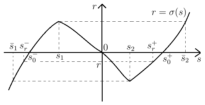
Figure 4. Diffusion flux $\sigma(s)$ of the non-Fourier type

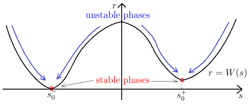
Figure 5. Double-well potential $W(s)$ of the non-Fourier type

We now formulate the result on global weak solutions $u$ to problem (1.1). An interesting feature of such a solution $u$ is that while it stabilizes to $\bar{u}_{0}$ in terms of the $L^{\infty}(\Omega)$-norm as $t\to\infty$, its spatial derivative $u_{x}$ concentrates on the set $\{s^{+}_{0},s^{-}_{0}\}$ in such a way that the energy $\mathcal{E}(u)$ converges in some sense to a specific number reflecting the allocation of double-well energy by the nonzero roots $s^{\pm}_{0}$ of $\sigma$ (see Figure 5).

Theorem 2.7 (Allocation of double-well energy).

There exist a strictly increasing sequence $0<t_{j}\to\infty$ and infinitely many global weak solutions $u$ to problem (1.1) satisfying the following properties:

• $\|u(\cdot,t)-\bar{u}_{0}\|_{\infty}\to 0$ as $t\to\infty,$

• $\big{\|}\mathrm{dist}\big{(}u_{x}(\cdot,t),\{s_{0}^{+},s_{0}^{-}\}\big{)}\big{\|}_{\infty}\to 0$ as $t\to\infty$ outside a null set in $(0,\infty)$,

• $\frac{1}{t_{j+1}-t_{j}}\int_{t_{j}}^{t_{j+1}}\mathcal{E}(u(\cdot,t))\,dt\to L\big{(}\lambda_{0}W(s^{+}_{0})+(1-\lambda_{0})W(s^{-}_{0})\big{)}$ as $j\to\infty$, where $\lambda_{0}:=\frac{-s^{-}_{0}}{s^{+}_{0}-s^{-}_{0}}\in(0,1)$.

Note that every constant function in $\Omega$ is a steady state solution to problem (1.1), which is unstable since its energy $LW(0)$ involves the local maximum value $W(0)>\max\{W(s^{+}_{0}),W(s^{-}_{0})\}$. However, by the above result, even for any constant initial datum, we still have global weak solutions to (1.1) with energy converging to a more stable level $L\big{(}\lambda_{0}W(s^{+}_{0})+(1-\lambda_{0})W(s^{-}_{0})\big{)}.$

3. Preliminaries and easy proofs

In this section, we prepare some useful results that are essential ingredients for proving our main results, and some of which may be of independent interest. In particular, as an easy consequence of the result in Subsection 3.1, we provide the proof of Theorems 2.1 and 2.3 in Subsection 3.2 concerning the existence and asymptotic behaviors of a unique global classical solution $u$ to problem (1.1) for suitable initial data $u_{0}$ when the diffusion flux $\sigma$ is either of the Höllig type or of the Perona-Malik type.

3.1. Parabolic equations

Here, we consider large time behaviors of a global classical solution to problem (1.1) when the problem is strictly parabolic. The following theorem will play the role of a major building block for constructing weak solutions of interest in our main results. Since it can be proved easily with the help of [10], we include its proof here.

Theorem 3.1.

Let $\sigma\in C^{3}(\mathbb{R})$ satisfy that $\sigma^{\prime}>0\;\;\mbox{in $\mathbb{R}$}.$ Then there exists a unique global solution $u\in C^{2,1}(\bar{\Omega}_{\infty})$ to problem (1.1) satisfying the following properties:

• for each $\tau>0$, $u\in C^{2+\alpha,1+\alpha/2}(\bar{\Omega}_{\tau})$,

• for all $t_{2}>t_{1}\geq 0,$

  $$\min_{\bar{\Omega}}u(\cdot,t_{1})\leq\min_{\bar{\Omega}}u(\cdot,t_{2})\leq\bar{u}_{0}\leq\max_{\bar{\Omega}}u(\cdot,t_{2})\leq\max_{\bar{\Omega}}u(\cdot,t_{1}),$$

• for all $t_{2}>t_{1}\geq 0,$

  $$\min_{\bar{\Omega}}u_{x}(\cdot,t_{1})\leq\min_{\bar{\Omega}}u_{x}(\cdot,t_{2})\leq 0\leq\max_{\bar{\Omega}}u_{x}(\cdot,t_{2})\leq\max_{\bar{\Omega}}u_{x}(\cdot,t_{1}),$$

• $\|u(\cdot,t)-\bar{u}_{0}\|_{W^{1,\infty}(\Omega)}\leq Ce^{-\gamma t}$ for all $t\geq 0$, where $0<\kappa<1$, $\lambda>0$, $m>1$,

  $$\theta:=\min_{[-\|u_{0}^{\prime}\|_{\infty}\frac{m}{m-1},\|u_{0}^{\prime}\|_{\infty}\frac{m}{m-1}]}\sigma^{\prime},\;\;\tilde{\theta}:=\max_{[-\|u_{0}^{\prime}\|_{\infty}\frac{m}{m-1},\|u_{0}^{\prime}\|_{\infty}\frac{m}{m-1}]}|\sigma^{\prime\prime}|,$$

  $$\gamma:=\frac{\kappa\theta\lambda^{2}e^{-\lambda L}}{\max\Big{\{}\frac{\|u_{0}^{\prime}\|_{\infty}\tilde{\theta}}{(1-\kappa)\theta}+1,m\Big{\}}-e^{-\lambda L}},$$

  and $C>0$ is some constant depending only on $u_{0}$, $\sigma$, $L$, $\kappa$, $\lambda$ and $m$.

Proof.

To start the proof, let us fix any numbers $0<\kappa<1$, $\lambda>0$ and $m>1$. Set $s_{0}=\|u_{0}^{\prime}\|_{\infty}\frac{m}{m-1}+1$, and choose a function $\tilde{\sigma}\in C^{3}(\mathbb{R})$ such that

(3.1) $$\left\{\begin{array}[]{l}\tilde{\sigma}(s)=\sigma(s)\;\;\forall s\in[-s_{0},s_{0}],\\ \lambda\leq\tilde{\sigma}^{\prime}(s)\leq\Lambda\;\;\forall s\in\mathbb{R},\\ \mbox{$\tilde{\sigma}^{\prime\prime\prime}$ is bounded in $\mathbb{R}$},\end{array}\right.$$

where $\Lambda\geq\lambda>0$ are some constants. Then it follows from [16, Theorem 13.24] that there exists a global solution $u\in C^{2,1}(\bar{\Omega}_{\infty})$ to problem (1.1), with $\sigma$ replaced by $\tilde{\sigma}$, such that $u\in C^{2+\alpha,1+\alpha/2}(\bar{\Omega}_{\tau})$ for each $\tau>0$.

We now check that $u$ is a unique global solution to problem (1.1), with original $\sigma$, satisfying (1)–(4).

Note first that (1) is satisfied as above. Next, according to [9, Lemma 2.2], we have an improved interior regularity of $u$ as $u\in C^{3+\beta,\frac{3+\beta}{2}}(\Omega\times(0,\tau])$ for all $\tau>0$, where $\beta\in(0,1)$ is some number. In particular, $\rho:=u_{x}\in C^{1,0}(\bar{\Omega}_{\infty})\cap C^{2,1}(\Omega_{\infty})$ solves the initial-boundary value problem:

(3.2) $$\left\{\begin{array}[]{ll}\rho_{t}=(\tilde{\sigma}(\rho))_{xx}&\mbox{in $\Omega\times(0,\infty)$,}\\ \rho=\rho_{0}&\mbox{on $\Omega\times\{t=0\}$,}\\ \rho=0&\mbox{on $\partial\Omega\times(0,\infty)$},\end{array}\right.$$

where $\rho_{0}:=u_{0}^{\prime}\in C^{1}(\bar{\Omega})$. So [10, Lemma 2.1] implies (3). Thanks to (3.1), it now follows from (3) that $u$ is a global solution to problem (1.1) with original $\sigma$. Also, from (3.1) and (3.2), it is easy to see that [10, Theorem 1.1] together with Poincaré’s inequality yields (4). Finally, uniqueness of such a solution $u$ to (1.1) and (2) are a consequence of [13, Propositions 2.3 and 2.4], respectively. ∎

3.2. Proof of Theorems 2.1 and 2.3

We first begin with the proof of Theorem 2.1. Fix a number $\bar{s}\in(M_{0},s_{1})$. We then choose a function $\tilde{\sigma}\in C^{3}(\mathbb{R})$ such that

$$\left\{\begin{array}[]{l}\mbox{$\tilde{\sigma}(s)=\sigma(s)$ $\forall s\in(-\infty,\bar{s}]$,}\\ \mbox{$\tilde{\sigma}^{\prime}>0$ in $\mathbb{R}$}.\end{array}\right.$$

Thanks to Theorem 3.1, there exists a unique global solution $u\in C^{2,1}(\bar{\Omega}_{\infty})$ to the problem

$$\left\{\begin{array}[]{ll}u_{t}=(\tilde{\sigma}(u_{x}))_{x}&\mbox{in $\Omega_{\infty}$,}\\ u=u_{0}&\mbox{on $\Omega\times\{t=0\}$,}\\ u_{x}=0&\mbox{on $\partial\Omega\times(0,\infty)$,}\end{array}\right.$$

satisfying (1)–(3). Moreover, by the validity of (3) and the choice of $\tilde{\sigma}$, $u$ is also a global solution to (1.1). Finally, (4) follows easily from (4) of Theorem 3.1

The proof of Theorem 2.3 is similar; the only difference is that we fix two numbers $\bar{s}_{1}\in(s_{1},m_{0})$, $\bar{s}_{2}\in(M_{0},s_{2})$ and choose a function $\tilde{\sigma}\in C^{3}(\mathbb{R})$ such that

$$\left\{\begin{array}[]{l}\mbox{$\tilde{\sigma}(s)=\sigma(s)$ $\forall s\in[\bar{s}_{1},\bar{s}_{2}]$,}\\ \mbox{$\tilde{\sigma}^{\prime}>0$ in $\mathbb{R}$}.\end{array}\right.$$

Then the rest can be finished as in the proof of Theorem 2.1 above; we do not repeat the details.

3.3. Baire’s category theorem

In this subsection, we prepare a suitable functional tool for solving a partial differential inclusion introduced in Subsection 3.5. We begin with the definition of a related terminology.

Definition 3.1.

Let $\mathfrak{X}$ and $\mathfrak{Y}$ be metric spaces. A map $f:\mathfrak{X}\to\mathfrak{Y}$ is called Baire-one if it is the pointwise limit of some sequence of continuous maps from $\mathfrak{X}$ into $\mathfrak{Y}$.

A version of Baire’s category theorem, regarding Baire-one maps, is the following.

Theorem 3.2 (Baire’s category theorem).

Let $\mathfrak{X}$ and $\mathfrak{Y}$ be metric spaces with $\mathfrak{X}$ complete. If $f:\mathfrak{X}\to\mathfrak{Y}$ is a Baire-one map, then the set of points of discontinuity for $f$, say $\mathfrak{D}_{f}$, is of the first category. Therefore, the set of points in $\mathfrak{X}$ at which $f$ is continuous, that is, $\mathfrak{C}_{f}:=\mathfrak{X}\setminus\mathfrak{D}_{f}$, is dense in $\mathfrak{X}$.

Our Baire-one maps to be used later are the gradient operators as follows.

Proposition 3.3.

Let $m$ and $n$ be any two positive integers. Let $U\subset\mathbb{R}^{n}$ be a bounded open set, and let $\mathfrak{X}\subset W^{1,\infty}(U;\mathbb{R}^{m})$ be equipped with the $L^{\infty}(U;\mathbb{R}^{m})$-metric. Then the gradient operator $\nabla:\mathfrak{X}\to L^{p}(U;\mathbb{M}^{m\times n})$ is a Baire-one map for each $p\in[1,\infty)$.

Since the proof of Theorem 3.2 and Proposition 3.3 can be found in [2, Chapter 10], we do not reproduce it here.

3.4. Rank-one smooth approximation

Here, we equip with an important but technical tool for local patching to be used in the proof of the density lemma, Lemma 3.5, stated in the next subsection. The following result is a refinement of the $(1+1)$-dimensional version of a combination of [12, Theorem 2.3 and Lemma 4.5], and its proof can be found in our recent paper [14, Theorem 6.1].

Lemma 3.4.

Let $Q=(x_{1},x_{2})\times(t_{1},t_{2})\subset\mathbb{R}^{2}$ be an open rectangle, where $x_{2}>x_{1}$ and $t_{2}>t_{1}$ are fixed reals. Given any $\lambda_{1}>0$, $\lambda_{2}>0$ and $\epsilon>0$, there exists a function $\omega=(\varphi,\psi)\in C^{\infty}_{c}(Q;\mathbb{R}^{2})$ such that

• $\|\omega\|_{L^{\infty}(Q)}<\epsilon$, $\|\varphi_{t}\|_{L^{\infty}(Q)}<\epsilon$, $\|\psi_{t}\|_{L^{\infty}(Q)}<\epsilon$,

• $-\lambda_{1}\leq\varphi_{x}\leq\lambda_{2}$ in $Q$,

• $\left\{\begin{array}[]{l}\big{|}|\{(x,t)\in Q\,|\,\varphi_{x}(x,t)=-\lambda_{1}\}|-\frac{\lambda_{2}}{\lambda_{1}+\lambda_{2}}|Q|\big{|}<\epsilon,\\ \big{|}|\{(x,t)\in Q\,|\,\varphi_{x}(x,t)=\lambda_{2}\}|-\frac{\lambda_{1}}{\lambda_{1}+\lambda_{2}}|Q|\big{|}<\epsilon,\end{array}\right.$

• $\psi_{x}=\varphi$ in $Q$, and

• $\int_{x_{1}}^{x_{2}}\varphi(x,t)\,dx=0$ for all $t_{1}<t<t_{2}$.

3.5. Phase transition as a differential inclusion

In proving Theorems 2.2, 2.4, 2.5, 2.6 and 2.7, we will keep repeatedly solving a certain partial differential inclusion in the framework of Baire’s category method. To avoid an unnecessary repetition, we separate a germ of common analysis into this subsection and make use of it whenever it is needed.

3.5.1. Initial definitions

Let $r_{1}<r_{2}$ be any two fixed numbers, and let $g^{\pm}=g^{\pm}_{r_{1},r_{2}}\in C([r_{1},r_{2}])$ be functions such that

$$g^{-}(r)<g^{+}(r)\;\;\forall r\in[r_{1},r_{2}].$$

Let $\tilde{K}^{\pm}=\tilde{K}_{g^{\pm}}$ denote the graph of $g^{\pm}$; that is,

$$\tilde{K}^{\pm}=\big{\{}(g^{\pm}(r),r)\in\mathbb{R}^{2}\,|\,r_{1}\leq r\leq r_{2}\big{\}}.$$

Set $\tilde{K}=\tilde{K}_{g^{+},g^{-}}=\tilde{K}^{+}\cup\tilde{K}^{-}$. Let $\tilde{U}=\tilde{U}_{g^{+},g^{-}}$ be the bounded domain in $\mathbb{R}^{2}$ given by

$$\tilde{U}=\big{\{}(\lambda g^{-}(r)+(1-\lambda)g^{+}(r),r)\,|\,r_{1}<r<r_{2},0<\lambda<1\big{\}}.$$

For each $u\in\mathbb{R}$, define the matrix sets

$$\begin{split}K(u)=K_{g^{+},g^{-}}(u)&=\left\{\begin{pmatrix}s&c\\ u&r\end{pmatrix}\in\mathbb{M}^{2\times 2}\,\Big{|}\,(s,r)\in\tilde{K},c\in\mathbb{R}\right\},\\ U(u)=U_{g^{+},g^{-}}(u)&=\left\{\begin{pmatrix}s&c\\ u&r\end{pmatrix}\in\mathbb{M}^{2\times 2}\,\Big{|}\,(s,r)\in\tilde{U},c\in\mathbb{R}\right\}.\end{split}$$

3.5.2. Related differential inclusion

We consider the inhomogeneous partial differential inclusion

(3.3) $$\nabla w(x,t)\in K(u(x,t)),\;\;\mbox{a.e. $(x,t)\in Q$},$$

where $Q\subset\mathbb{R}^{2}$ is a bounded open set, $w=(u,v):Q\to\mathbb{R}^{2}$ is a Lipschitz function, and $\nabla w=\begin{pmatrix}u_{x}&u_{t}\\ v_{x}&v_{t}\end{pmatrix}$ is the Jacobian matrix of $w$.

We say that a Lipschitz function $w:Q\to\mathbb{R}^{2}$ is a subsolution of differential inclusion (3.3) if

$$\nabla w(x,t)\in K(u(x,t))\cup U(u(x,t)),\;\;\mbox{a.e. $(x,t)\in Q$},$$

and it is a strict subsolution of (3.3) if

$$\nabla w(x,t)\in U(u(x,t)),\;\;\mbox{a.e. $(x,t)\in Q$}.$$

Let $w=(u,v):Q\to\mathbb{R}^{2}$ be a subsolution of differential inclusion (3.3). For a.e. $(x,t)\in Q$, we can define the quantity

$$Z_{w}(x,t)=Z^{Q}_{g^{+},g^{-};w}(x,t)=\frac{u_{x}(x,t)-g^{-}(v_{t}(x,t))}{g^{+}(v_{t}(x,t))-g^{-}(v_{t}(x,t))}\in[0,1].$$

For each non-null subset $E$ of $Q$, we then define the transition gauge of $w$ over $E$ by

$$\Gamma_{w}^{E}=\Gamma^{E}_{g^{+},g^{-};w}=\frac{1}{|E|}\int_{E}Z_{w}(x,t)\,dxdt\in[0,1].$$

This gauge measures the inclination of the diagonal $(u_{x},v_{t})$ of $\nabla w$ over $E$ towards the right branch $\tilde{K}^{+}$ of $\tilde{K}$; for instance, it is easy to see that

$$\Gamma_{w}^{E}=1 \Longleftrightarrow (u_{x},v_{t})\in\tilde{K}^{+} E$$ a.e. in

and that

$$\mbox{$\Gamma_{w}^{E}=0$ $\Longleftrightarrow$ $(u_{x},v_{t})\in\tilde{K}^{-}$ a.e. in $E$}.$$

Note also that if $w$ is a strict subsolution of (3.3), then $0<\Gamma_{w}^{E}<1$ for every non-null subset $E$ of $Q$.

3.5.3. Generic setup and density lemma

Let $b>0$ be any fixed number. For each $u\in\mathbb{R}$, define the matrix sets

$$\begin{split}K_{b}(u)&=K_{g^{+},g^{-};b}(u)=\left\{\begin{pmatrix}s&c\\ u&r\end{pmatrix}\in\mathbb{M}^{2\times 2}\,\Big{|}\,(s,r)\in\tilde{K},|c|\leq b\right\},\\ U_{b}(u)&=U_{g^{+},g^{-};b}(u)=\left\{\begin{pmatrix}s&c\\ u&r\end{pmatrix}\in\mathbb{M}^{2\times 2}\,\Big{|}\,(s,r)\in\tilde{U},|c|<b\right\}.\end{split}$$

Let $Q\subset\mathbb{R}^{2}$ be a bounded open set, and let $w^{*}=(u^{*},v^{*})\in(C^{2,1}\times C^{3,1})(\bar{Q}):=C^{2,1}(\bar{Q})\times C^{3,1}(\bar{Q})$ be a Lipschitz function such that

$$\nabla w^{*}\in U_{b}(u^{*})\;\;\mbox{in $Q$};$$

then $w^{*}$ is a strict subsolution of differential inclusion (3.3) so that $0<\Gamma_{w^{*}}^{E}<1$ for each non-null subset $E$ of $Q$.

Let $\epsilon>0$ be any fixed number. We define a class $\mathcal{A}=\mathcal{A}_{g^{+},g^{-},b,w^{*},Q,\epsilon}$ of strict subsolutions of (3.3) by

$$\mathcal{A}=\left\{\begin{array}[]{l}w=(u,v)\in\\ (C^{2,1}\times C^{3,1})(\bar{Q})\end{array}\,\Bigg{|}\,\begin{array}[]{l}\mbox{$w$ is Lipschitz in $Q$, $w=w^{*}$ in $Q\setminus\bar{Q}^{w}$}\\ \mbox{for some open set $Q^{w}\subset\subset Q$ with $|\partial Q^{w}|=0$,}\\ \mbox{$\|u-u^{*}\|_{L^{\infty}(Q)}<\epsilon/2$, $\|u_{t}-u_{t}^{*}\|_{L^{\infty}(Q)}<\epsilon/2$,}\\ \mbox{$\nabla w\in U_{b}(u)$ in $Q$, $|\Gamma^{Q}_{w}-\Gamma^{Q}_{w^{*}}|<\epsilon/2$}\end{array}\right\};$$

then $w^{*}\in\mathcal{A}$ so that $\mathcal{A}\neq\emptyset$. Next, for each $\delta>0$, we define a subclass $\mathcal{A}_{\delta}=\mathcal{A}_{g^{+},g^{-},b,w^{*},Q,\epsilon;\delta}$ of $\mathcal{A}$ by

$$\mathcal{A}_{\delta}=\left\{w\in\mathcal{A}\,\Big{|}\,\int_{Q}\mathrm{dist}\big{(}\nabla w(x,t),K_{b}(u(x,t))\big{)}\,dxdt\leq\delta|Q|\right\}.$$

We now state the pivotal density lemma that will be used throughout the rest of the paper.

Lemma 3.5.

For each $\delta>0$, $\mathcal{A}_{\delta}$ is dense in $\mathcal{A}$ under the $L^{\infty}(Q)$-norm.

The proof of this lemma is so long and complicated that we postpone it to the last section, Section 8.

4. Eventual smoothing for Höllig type equations

This section is devoted to proving Theorem 2.2, that is, the existence of eventually smooth global weak solutions $u$ to problem (1.1) for all initial data $u_{0}$ with $M_{0}>\bar{s}_{1}$ when the diffusion flux $\sigma$ is of the Höllig type.

Following the notation and setup in Subsection 3.5, we divide the proof into several steps.

Setup and subsolution

Let

$$g^{\pm}=g^{\pm}_{r_{1},r_{2}}=(\sigma|_{[s^{\pm}_{r_{1}},s^{\pm}_{r_{2}}]})^{-1}:[r_{1},r_{2}]\to[s^{\pm}_{r_{1}},s^{\pm}_{r_{2}}];$$

then $g^{-}\leq g^{-}(r_{2})=s^{-}_{r_{2}}<s^{+}_{r_{1}}=g^{+}(r_{1})\leq g^{+}$ on $[r_{1},r_{2}]$. Next, we choose a function $\tilde{\sigma}=\tilde{\sigma}_{r_{1},r_{2}}\in C^{3}(\mathbb{R})$ (see Figure 6) such that

(4.1) $$\left\{\begin{array}[]{l}\tilde{\sigma}=\sigma\;\;\mbox{on $(-\infty,s^{-}_{r_{1}}]\cup[s^{+}_{r_{2}},\infty)$},\\ \tilde{\sigma}<\sigma\;\;\mbox{on $(s^{-}_{r_{1}},s^{-}_{r_{2}}]$},\;\tilde{\sigma}>\sigma\;\;\mbox{on $[s^{+}_{r_{1}},s^{+}_{r_{2}})$},\\ \tilde{\sigma}^{\prime}>0\;\;\mbox{in $\mathbb{R}$.}\end{array}\right.$$

Thanks to Theorem 3.1, there exists a unique global solution $u^{*}\in C^{2,1}(\bar{\Omega}_{\infty})$ to problem (1.1), with $\sigma$ replaced by $\tilde{\sigma}$, satisfying (6)–(9), where the constants $\kappa$, $\lambda$ and $m$ are fixed as in (4) of Theorem 3.1 to yield (9).

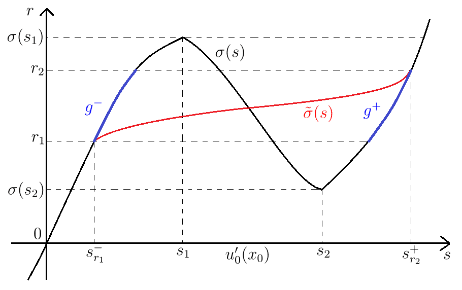
Figure 6. Modified flux $\tilde{\sigma}(s)$

Now, let $Q_{1}$, $Q_{2}$ and $F^{\pm}$ be defined as in the statement of the theorem. It then follows from (9) that $Q_{1}\cup Q_{2}\cup F^{+}\cup F^{-}$ is bounded. Also, this set has a positive distance to the vertical boundary $\partial\Omega\times[0,\infty)$ since $u^{*}_{x}$ vanishes on $\partial\Omega\times[0,\infty)$ and is continuous on $\bar{\Omega}_{\infty};$ thus (4) holds. Since $s^{-}_{r_{1}}<u_{0}^{\prime}(x_{0})<s^{+}_{r_{2}}$, we have $Q_{1}\neq\emptyset$ so that $0<\sup_{(x,t)\in Q_{1}}t=:t_{1}<\infty$ by (4). This together with (8) and (9) implies (5).

Let $Q=Q_{1}$ and $b=\|u^{*}_{t}\|_{L^{\infty}(Q)}+1.$ With the functions $g^{\pm}$ defined above, for each $u\in\mathbb{R}$, let $K_{b}(u)=K_{g^{+},g^{-};b}(u)$ and $U_{b}(u)=U_{g^{+},g^{-};b}(u)$ be given as in Subsection 3.5. Define an auxiliary function $v^{*}$ by

$$v^{*}(x,t)=\int_{0}^{t}\tilde{\sigma}(u_{x}^{*}(x,\tau))\,d\tau+\int_{0}^{x}u_{0}(y)\,dy\;\;\forall(x,t)\in\Omega_{\infty};$$

then

(4.2) $$\left\{\begin{array}[]{l}v^{*}_{t}=\tilde{\sigma}(u^{*}_{x})\\ v^{*}_{x}=u^{*}\end{array}\right.\mbox{in $\Omega_{\infty}$},$$

and so $w^{*}:=(u^{*},v^{*})\in(C^{2,1}\times C^{3,1})(\bar{\Omega}_{\infty})$. From this, (4.1) and the definition of $b$, we have

$$\nabla w^{*}\in U_{b}(u^{*})\;\;\mbox{in $Q$};$$

thus $w^{*}|_{Q}$ becomes a strict subsolution of differential inclusion (3.3) so that $0<\Gamma^{Q}_{w^{*}}<1$, where the gauge operator $\Gamma^{Q}_{\cdot}=\Gamma^{Q}_{g^{+},g^{-};\cdot}$ is given as in Subsection 3.5.

Admissible class

Fix any $\epsilon>0$. Following the above, let $\mathcal{A}=\mathcal{A}_{g^{+},g^{-},b,w^{*},Q,\epsilon}$ and $\mathcal{A}_{\delta}=\mathcal{A}_{g_{+},g_{-},b,w^{*},Q,\epsilon;\delta}$ $(\delta>0)$ be defined as in Subsection 3.5. Set $t_{2}=t_{1}+1$, where $t_{1}>0$ is as above; then $Q\subset\Omega_{t_{2}-1}\subset\Omega_{t_{2}}$. We now define a class $\mathfrak{A}$ of admissible functions by

$$\mathfrak{A}=\left\{\begin{array}[]{l}w=(u,v)\in\\ (C^{2,1}\times C^{3,1})(\bar{\Omega}_{t_{2}})\end{array}\,\Big{|}\,\begin{array}[]{l}\mbox{$w=w^{*}$ in $\Omega_{t_{2}}\setminus Q$,}\\ w|_{Q}\in\mathcal{A}\par\end{array}\right\};$$

then $w^{*}\in\mathfrak{A}$ so that $\mathfrak{A}\neq\emptyset$. Next, for each $\delta>0$, let $\mathfrak{A}_{\delta}$ be the subclass of functions $w\in\mathfrak{A}$ such that $w|_{Q}\in\mathcal{A}_{\delta}$.

Baire’s category method

Let $\mathfrak{X}$ denote the closure of $\mathfrak{A}$ in the space $L^{\infty}(\Omega_{t_{2}};\mathbb{R}^{2})$; then $(\mathfrak{X},L^{\infty})$ becomes a nonempty complete metric space. From the definition of $\mathfrak{A}$, it is easily checked that

$$\mathfrak{X}\subset w^{*}+W^{1,\infty}_{0}(\Omega_{t_{2}};\mathbb{R}^{2}).$$

By Proposition 3.3, the space-time gradient operator $\nabla:\mathfrak{X}\to L^{1}(\Omega_{t_{2}};\mathbb{M}^{2\times 2})$ is a Baire-one map, and thus it follows from the Baire category theorem, Theorem 3.2, that the set of points at which $\nabla$ is continuous, say $\mathfrak{C}_{\nabla}$, is dense in $\mathfrak{X}$.

Solutions from $\mathfrak{C}_{\nabla}$

Let $w=(u,v)\in\mathfrak{C}_{\nabla},$ and extend it from $\Omega_{t_{2}}$ to $\Omega_{\infty}$ by setting $w=w^{*}$ in $\Omega_{\infty}\setminus\Omega_{t_{2}}$. We now show that $u$ is a global weak solution to problem (1.1) satisfying (1)–(3).

Note first that from Lemma 3.5 and the density of $\mathfrak{A}$ in $\mathfrak{X}$, $\mathfrak{A}_{1/j}$ is dense in $\mathfrak{X}$ for each $j\in\mathbb{N}$. So we can take a sequence $w_{j}=(u_{j},v_{j})\in\mathfrak{A}_{1/j}$ such that $\|w_{j}-w\|_{L^{\infty}(\Omega_{t_{2}})}\to 0$ as $j\to\infty$. By the continuity of the operator $\nabla$ at $w$, we have $\nabla w_{j}\to\nabla w$ in $L^{1}(\Omega_{t_{2}};\mathbb{M}^{2\times 2})$ and hence pointwise a.e. in $\Omega_{t_{2}}$ after passing to a subsequence if necessary.

We state some properties of the function $w_{j}=(u_{j},v_{j})$ inherited from its membership $w_{j}\in\mathfrak{A}_{1/j}$:

(4.3) $$\left\{\begin{array}[]{l}w_{j}=(u_{j},v_{j})\in(C^{2,1}\times C^{3,1})(\bar{\Omega}_{t_{2}}),\\ \mbox{$w_{j}=w^{*}$ in $\Omega_{t_{2}}\setminus\bar{Q}^{w_{j}}$ for some open set $Q^{w_{j}}\subset\subset Q$ with $|\partial Q^{w_{j}}|=0$},\\ \|u_{j}-u^{*}\|_{L^{\infty}(Q)}<\epsilon/2,\;\|(u_{j})_{t}-u_{t}^{*}\|_{L^{\infty}(Q)}<\epsilon/2,\;|\Gamma^{Q}_{w_{j}}-\Gamma^{Q}_{w^{*}}|<\epsilon/2,\\ \mbox{$\nabla w_{j}\in U_{b}(u_{j})$ in $Q$, and}\\ \int_{Q}\mathrm{dist}\big{(}\nabla w_{j}(x,t),K_{b}(u_{j}(x,t))\big{)}\,dxdt\leq\frac{1}{j}|Q|.\end{array}\right.$$

We now check that $u$ satisfies (1)–(3). Letting $j\to\infty$ in (4.3), we get

$$\left\{\begin{array}[]{l}\mbox{$w=w^{*}$ in $\bar{\Omega}_{t_{2}}\setminus Q$,}\\ \|u-u^{*}\|_{L^{\infty}(Q)}\leq\epsilon/2,\;\|u_{t}-u_{t}^{*}\|_{L^{\infty}(Q)}\leq\epsilon/2;\end{array}\right.$$

thus (1) holds. We also have

$$\begin{split}\int_{Q}\mathrm{dist}\big{(}\nabla w_{j}&(x,t),K_{b}(u_{j}(x,t))\big{)}\,dxdt\\ &\to\int_{Q}\mathrm{dist}\big{(}\nabla w(x,t),K_{b}(u(x,t))\big{)}\,dxdt=0\end{split}$$

so that $\nabla w\in K_{b}(u)$ a.e. in $Q$. This inclusion implies that a.e. in $Q$,

(4.4) $$\left\{\begin{array}[]{l}v_{t}=\sigma(u_{x}),\\ u_{x}\in[s^{-}_{r_{1}},s^{-}_{r_{2}}]\cup[s^{+}_{r_{1}},s^{+}_{r_{2}}].\end{array}\right.$$

From (4.3), we have $(u_{j})_{x}=s^{+}_{r_{2}}$ in $F^{+}$ and $(u_{j})_{x}=s^{-}_{r_{1}}$ in $F^{-}$. Letting $j\to\infty$, we have $u_{x}=s^{+}_{r_{2}}$ a.e. in $F^{+}$ and $u_{x}=s^{-}_{r_{1}}$ a.e. in $F^{-}$; this and (4.4) yield (2). Also, letting $j\to\infty$ in (4.3), we have $|\Gamma^{Q}_{w}-\Gamma^{Q}_{w^{*}}|\leq\epsilon/2<\epsilon$. Without loss of generality, we can assume $0<\epsilon<\min\{\Gamma^{Q}_{w^{*}},1-\Gamma^{Q}_{w^{*}}\}$ so that $0<\Gamma^{Q}_{w}<1$. This and (4.4) thus imply (3).

For a later use, note from (4.3) that $(v_{j})_{t}=v^{*}_{t}$ and $(u_{j})_{x}=u^{*}_{x}\not\in(s^{-}_{r_{1}},s^{+}_{r_{2}})$ in $\Omega_{t_{2}}\setminus Q$, and so by (4.1) and (4.2),

(4.5) $$v_{t}=v^{*}_{t}=\tilde{\sigma}(u^{*}_{x})=\sigma(u^{*}_{x})=\sigma(u_{x})\;\;\mbox{a.e. in $\Omega_{t_{2}}\setminus Q$}.$$

By (4.2) and (4.3), we get $(v_{j})_{x}=u_{j}$ in $\Omega_{t_{2}}$; thus we have

(4.6) $$v_{x}=u\;\;\mbox{a.e. in $\Omega_{t_{2}}$}.$$

Let us now check that $u$ is a global weak solution to problem (1.1). To do this, let $\zeta\in C^{\infty}(\bar{\Omega}_{\infty})$ and $\tau\in[0,\infty)$. Assume first that $\tau\leq t_{2}$. From (4.2) and (4.3), we then have

$$\begin{split}&\int_{0}^{\tau}\int_{0}^{L}u_{j}\zeta_{t}\,dxdt=\int_{0}^{\tau}\int_{0}^{L}(v_{j})_{x}\zeta_{t}\,dxdt\\ &=-\int_{0}^{\tau}\int_{0}^{L}(v_{j})_{xt}\zeta\,dxdt+\int_{0}^{L}\big{(}(v_{j})_{x}(x,\tau)\zeta(x,\tau)-(v_{j})_{x}(x,0)\zeta(x,0)\big{)}\,dx\\ &=\int_{0}^{\tau}\int_{0}^{L}(v_{j})_{t}\zeta_{x}\,dxdt-\int_{0}^{\tau}\big{(}(v_{j})_{t}(L,t)\zeta(L,t)-(v_{j})_{t}(0,t)\zeta(0,t)\big{)}\,dt\\ &\;\;\;\;+\int_{0}^{L}\big{(}(v_{j})_{x}(x,\tau)\zeta(x,\tau)-(v_{j})_{x}(x,0)\zeta(x,0)\big{)}\,dx\\ &=\int_{0}^{\tau}\int_{0}^{L}(v_{j})_{t}\zeta_{x}\,dxdt-\int_{0}^{\tau}\big{(}v^{*}_{t}(L,t)\zeta(L,t)-v^{*}_{t}(0,t)\zeta(0,t)\big{)}\,dt\\ &\;\;\;\;+\int_{0}^{L}\big{(}u_{j}(x,\tau)\zeta(x,\tau)-u_{0}(x)\zeta(x,0)\big{)}\,dx.\end{split}$$

Let $j\to\infty$; then from (4.4), (4.5) and $v^{*}_{t}=\tilde{\sigma}(u^{*}_{x})=0$ on $\partial\Omega\times[0,\infty)$, we have

$$\begin{split}\int_{0}^{\tau}\int_{0}^{L}u\zeta_{t}&\,dxdt=\int_{0}^{\tau}\int_{0}^{L}v_{t}\zeta_{x}\,dxdt+\int_{0}^{L}\big{(}u(x,\tau)\zeta(x,\tau)-u_{0}(x)\zeta(x,0)\big{)}\,dx\\ &=\int_{0}^{\tau}\int_{0}^{L}\sigma(u_{x})\zeta_{x}\,dxdt+\int_{0}^{L}\big{(}u(x,\tau)\zeta(x,\tau)-u_{0}(x)\zeta(x,0)\big{)}\,dx;\end{split}$$

hence (1.2) holds.

Next, assume that $\tau>t_{2}.$ Since $u=u^{*}$ and $u^{*}_{x}\leq s^{-}_{r_{1}}$ on $\bar{\Omega}\times[t_{2},\infty)$ and $u^{*}$ is a global classical solution to problem (1.1) with $\sigma$ replaced by $\tilde{\sigma}$, it follows from (4.1) that

$$\begin{split}\int_{0}^{L}\big{(}&u(x,\tau)\zeta(x,\tau)-u(x,t_{2})\zeta(x,t_{2})\big{)}\,dx\\ &=\int_{0}^{L}\big{(}u^{*}(x,\tau)\zeta(x,\tau)-u^{*}(x,t_{2})\zeta(x,t_{2})\big{)}\,dx\\ &=\int_{t_{2}}^{\tau}\int_{0}^{L}\big{(}u^{*}\zeta_{t}-\tilde{\sigma}(u^{*}_{x})\zeta_{x}\big{)}\,dxdt=\int_{t_{2}}^{\tau}\int_{0}^{L}\big{(}u\zeta_{t}-\sigma(u_{x})\zeta_{x}\big{)}\,dxdt.\end{split}$$

Combining this with the previous case with $\tau=t_{2}$, we obtain (1.2); therefore, $u$ is a global weak solution to (1.1).

Infinitely many solutions

We have shown above that the first component $u$ of each function $w=(u,v)\in\mathfrak{C}_{\nabla}$ with common extension $u=u^{*}$ in $\Omega_{\infty}\setminus\Omega_{t_{2}}$ is a global weak solution to problem (1.1) satisfying (1)–(3). It only remains to verify that $\mathfrak{C}_{\nabla}$ contains infinitely many functions and that no two different functions in $\mathfrak{C}_{\nabla}$ have the first component that are identical. Suppose first on the contrary that $\mathfrak{C}_{\nabla}$ has only finitely many functions. Then

$$\mathfrak{C}_{\nabla}=\bar{\mathfrak{C}}_{\nabla}=\mathfrak{X}=\bar{\mathfrak{A}}=\mathfrak{A}\ni w^{*}=(u^{*},v^{*}),$$

where the closure is with respect to the $L^{\infty}(\Omega_{t_{2}};\mathbb{R}^{2})$-norm. By the above result, we now have that $u^{*}$ itself is a global weak solution to (1.1) satisfying (1)–(3); clearly, this is a contradiction. Thus, $\mathfrak{C}_{\nabla}$ contains infinitely many functions. Next, let $w_{1}=(u_{1},v_{1}),w_{2}=(u_{2},v_{2})\in\mathfrak{C}_{\nabla}.$ It is sufficient to show that

$$u_{1}=u_{2}\;\;\mbox{in $\Omega_{t_{2}}$}\;\;\Longleftrightarrow\;\;v_{1}=v_{2}\;\;\mbox{in $\Omega_{t_{2}}$}.$$

If $u_{1}=u_{2}$ in $\Omega_{t_{2}}$, then by (4.6), we have $(v_{1})_{x}=u_{1}=u_{2}=(v_{2})_{x}$ a.e. in $\Omega_{t_{2}}$. Since $v_{1}=v_{2}=v^{*}$ on $\partial\Omega_{t_{2}}$, we get $v_{1}=v_{2}$ in $\Omega_{t_{2}}.$ The converse is also easy to check; we skip this.

The proof of Theorem 2.2 is now complete.

5. Eventual smoothing for Perona-Malik type equations

In this section, we prove the existence of eventually smooth global weak solutions $u$ to problem (1.1) for all nonconstant initial data $u_{0}$ when the diffusion flux $\sigma$ is of the Perona-Malik type. We first provide the proof of Theorem 2.4, which handles Case 1: $m_{0}<0<M_{0}.$ Since the proof of Theorem 2.5 for Case 2: $0=m_{0}<M_{0}$ is very similar to and even simpler than that of Theorem 2.4, we only give a sketch for the proof at the end of the section. Likewise, for Case 3: $m_{0}<M_{0}=0$ that we do not state as a theorem, one can easily adapt the proof of Theorem 2.4 to deduce the expected result.

Proof of Theorem 2.4.

Following the notation and setup in Subsection 3.5, we divide the proof into several steps.

Setup and subsolution

Let

$$\begin{split}g_{1}^{+}&=g^{+}_{r_{1}^{\prime},r_{1}}=(\sigma|_{[s^{+}_{r_{1}^{\prime}},s^{+}_{r_{1}}]})^{-1}:[r_{1}^{\prime},r_{1}]\to[s^{+}_{r_{1}^{\prime}},s^{+}_{r_{1}}],\\ g_{1}^{-}&=g^{-}_{r_{1}^{\prime},r_{1}}=(\sigma|_{[s^{-}_{r_{1}},s^{-}_{r_{1}^{\prime}}]})^{-1}:[r_{1}^{\prime},r_{1}]\to[s^{-}_{r_{1}},s^{-}_{r_{1}^{\prime}}],\\ g_{2}^{+}&=g^{+}_{r_{2},r_{2}^{\prime}}=(\sigma|_{[s^{+}_{r_{2}^{\prime}},s^{+}_{r_{2}}]})^{-1}:[r_{2},r_{2}^{\prime}]\to[s^{+}_{r_{2}^{\prime}},s^{+}_{r_{2}}],\\ g_{2}^{-}&=g^{-}_{r_{2},r_{2}^{\prime}}=(\sigma|_{[s^{-}_{r_{2}},s^{-}_{r_{2}^{\prime}}]})^{-1}:[r_{2},r_{2}^{\prime}]\to[s^{-}_{r_{2}},s^{-}_{r_{2}^{\prime}}];\end{split}$$

then

$$\begin{split}g_{1}^{-}\leq g_{1}^{-}(r_{1}^{\prime})=s^{-}_{r_{1}^{\prime}}&<s^{+}_{r_{1}^{\prime}}=g_{1}^{+}(r_{1}^{\prime})\leq g_{1}^{+}\;\;\mbox{on $[r_{1}^{\prime},r_{1}]$},\\ g_{2}^{-}\leq g_{2}^{-}(r_{2}^{\prime})=s^{-}_{r_{2}^{\prime}}&<s^{+}_{r_{2}^{\prime}}=g_{2}^{+}(r_{2}^{\prime})\leq g_{2}^{+}\;\;\mbox{on $[r_{2},r_{2}^{\prime}]$}.\end{split}$$

Next, choose a function $\tilde{\sigma}=\tilde{\sigma}_{r_{1},r_{1}^{\prime},r_{2},r_{2}^{\prime}}\in C^{3}(\mathbb{R})$ (see Figure 7) such that

(5.1) $$\left\{\begin{array}[]{l}\mbox{$\tilde{\sigma}=\sigma$ on $[s^{+}_{r_{1}},s^{-}_{r_{2}}]$,}\\ \mbox{$\tilde{\sigma}<\min\{\sigma,r_{2}^{\prime}\}$ on $(s^{-}_{r_{2}},M_{0}]$,}\\ \mbox{$\tilde{\sigma}>\max\{\sigma,r_{1}^{\prime}\}$ on $[m_{0},s^{+}_{r_{1}})$,}\\ \mbox{$\tilde{\sigma}^{\prime}>0$ in $\mathbb{R}$.}\end{array}\right.$$

Owing to Theorem 3.1, there exists a unique global solution $u^{*}\in C^{2,1}(\bar{\Omega}_{\infty})$ to problem (1.1), with $\sigma$ replaced by $\tilde{\sigma}$, satisfying (5)–(8), where the constants $\kappa$, $\lambda$ and $m$ are fixed as in (4) of Theorem 3.1 to imply (8).

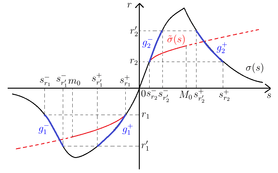
Figure 7. Modified flux $\tilde{\sigma}(s)$

Now, let $Q_{1}$, $Q_{2}$, $F_{1}$ and $F_{2}$ be defined as in the statement of the theorem. From (8), it follows that $Q_{1}\cup Q_{2}\cup F_{1}\cup F_{2}$ is bounded. This set also has a positive distance to the vertical boundary $\partial\Omega\times[0,\infty)$, since $u_{x}^{*}$ vanishes on $\partial\Omega\times[0,\infty)$ and is continuous on $\bar{\Omega}_{\infty}$; thus (4) is valid.

Let $b=\|u^{*}_{t}\|_{L^{\infty}(Q_{1}\cup Q_{2})}+1$. With the functions $g_{i}^{\pm}$ $(i=1,2)$ defined above, for each $u\in\mathbb{R},$ let $K_{i,b}(u)=K_{g_{i}^{+},g_{i}^{-};b}(u)$ and $U_{i,b}(u)=U_{g_{i}^{+},g_{i}^{-};b}(u)$ be given as in Subsection 3.5. Define an auxiliary function $v^{*}$ by

$$v^{*}(x,t)=\int_{0}^{t}\tilde{\sigma}(u^{*}_{x}(x,\tau))\,d\tau+\int_{0}^{x}u_{0}(y)\,dy\;\;\forall(x,t)\in\Omega_{\infty};$$

then

(5.2) $$\left\{\begin{array}[]{l}v^{*}_{t}=\tilde{\sigma}(u^{*}_{x})\\ v^{*}_{x}=u^{*}\end{array}\mbox{in $\Omega_{\infty}$,}\right.$$

so that $w^{*}:=(u^{*},v^{*})\in(C^{2,1}\times C^{3,1})(\bar{\Omega}_{\infty})$. From this, (5.1) and the definition of $b$, it follows that for $i=1,2$,

$$\nabla w^{*}\in U_{i,b}(u^{*})\;\;\mbox{in $Q_{i}$};$$

thus $w^{*}|_{Q_{i}}$ is a strict subsolution of differential inclusion (3.3) with $Q=Q_{i}$, and so $0<\Gamma^{Q_{i}}_{w^{*}}<1$, where the gauge operator $\Gamma^{Q_{i}}_{\cdot}=\Gamma^{Q_{i}}_{g_{i}^{+},g_{i}^{-};\cdot}$ is given as in Subsection 3.5.

Admissible class

Fix any $\epsilon>0$. Following the above notation, for $i=1,2$, let $\mathcal{A}_{i}=\mathcal{A}_{g_{i}^{+},g_{i}^{-},b,w^{*},Q_{i},\epsilon}$ and $\mathcal{A}_{i,\delta}=\mathcal{A}_{g_{i}^{+},g_{i}^{-},b,w^{*},Q_{i},\epsilon;\delta}$ $(\delta>0)$ be defined as in Subsection 3.5. Set $t_{1}=\sup_{(x,t)\in Q_{1}\cup Q_{2}}t+1$; then $Q_{1}\cup Q_{2}\subset\Omega_{t_{1}-1}\subset\Omega_{t_{1}}.$ We now define a class $\mathfrak{A}$ of admissible functions by

$$\mathfrak{A}=\left\{\begin{array}[]{l}w=(u,v)\in\\ (C^{2,1}\times C^{3,1})(\bar{\Omega}_{t_{1}})\end{array}\,\Big{|}\,\begin{array}[]{l}\mbox{$w=w^{*}$ in $\Omega_{t_{1}}\setminus(Q_{1}\cup Q_{2})$,}\\ \mbox{$w|_{Q_{i}}\in\mathcal{A}_{i}$ for $i=1,2$}\end{array}\right\};$$

then $w^{*}\in\mathfrak{A}$, and so $\mathfrak{A}\neq\emptyset.$ Also, for each $\delta>0$, let $\mathfrak{A}_{\delta}$ be the subclass of functions $w\in\mathfrak{A}$ such that $w|_{Q_{i}}\in\mathcal{A}_{i,\delta}$ for $i=1,2$.

Baire’s category method

Let $\mathfrak{X}$ denote the closure of $\mathfrak{A}$ in the space $L^{\infty}(\Omega_{t_{1}};\mathbb{R}^{2})$; then $(\mathfrak{X},L^{\infty})$ becomes a nonempty complete metric space. From the definition of $\mathfrak{A}$, it is easily checked that

$$\mathfrak{X}\subset w^{*}+W^{1,\infty}_{0}(\Omega_{t_{1}};\mathbb{R}^{2}).$$

As in the proof of Theorem 2.2, we know that the set of points of continuity for the space-time gradient operator $\nabla:\mathfrak{X}\to L^{1}(\Omega_{t_{1}};\mathbb{M}^{2\times 2})$, say $\mathfrak{C}_{\nabla},$ is dense in $\mathfrak{X}$.

Solutions from $\mathfrak{C}_{\nabla}$

Let $w=(u,v)\in\mathfrak{C}_{\nabla},$ and extend it from $\Omega_{t_{1}}$ to $\Omega_{\infty}$ by letting $w=w^{*}$ in $\Omega_{\infty}\setminus\Omega_{t_{1}}$. We now show that $u$ is a global weak solution to problem (1.1) satisfying (1)–(3).

Note first that by Lemma 3.5 and the density of $\mathfrak{A}$ in $\mathfrak{X}$, $\mathfrak{A}_{1/j}$ is dense in $\mathfrak{X}$ for each $j\in\mathbb{N}$. So we can take a sequence $w_{j}=(u_{j},v_{j})\in\mathfrak{A}_{1/j}$ such that $\|w_{j}-w\|_{L^{\infty}(\Omega_{t_{1}})}\to 0$ as $j\to\infty$. By the continuity of the operator $\nabla$ at $w$, we have $\nabla w_{j}\to\nabla w$ in $L^{1}(\Omega_{t_{1}};\mathbb{M}^{2\times 2})$ and hence pointwise a.e. in $\Omega_{t_{1}}$ after passing to a subsequence if necessary.

We now state some properties of the function $w_{j}=(u_{j},v_{j})$ inherited from its membership $w_{j}\in\mathfrak{A}_{1/j}$:

(5.3) $$\left\{\begin{array}[]{l}w_{j}=(u_{j},v_{j})\in(C^{2,1}\times C^{3,1})(\bar{\Omega}_{t_{1}}),\\ \mbox{$w_{j}=w^{*}$ in $\Omega_{t_{1}}\setminus(\bar{Q}_{1}^{w_{j}}\cup\bar{Q}_{2}^{w_{j}})$ for some open sets $Q_{1}^{w_{j}}\subset\subset Q_{1}$}\\ \mbox{\;\;\;\;\;and $Q_{2}^{w_{j}}\subset\subset Q_{2}$ with $|\partial Q_{1}^{w_{j}}|=|\partial Q_{2}^{w_{j}}|=0$},\\ \|u_{j}-u^{*}\|_{L^{\infty}(Q_{i})}<\epsilon/2,\;\|(u_{j})_{t}-u_{t}^{*}\|_{L^{\infty}(Q_{i})}<\epsilon/2,\\ \mbox{\;\;\;\, $|\Gamma^{Q_{i}}_{w_{j}}-\Gamma^{Q_{i}}_{w^{*}}|<\epsilon/2$ for $i=1,2$},\\ \mbox{$\nabla w_{j}\in U_{i,b}(u_{j})$ in $Q_{i}$ for $i=1,2$, and}\\ \mbox{$\int_{Q_{i}}\mathrm{dist}\big{(}\nabla w_{j}(x,t),K_{i,b}(u_{j}(x,t))\big{)}\,dxdt\leq\frac{1}{j}|Q_{i}|$ for $i=1,2$}.\end{array}\right.$$

Let us now check that $u$ satisfies (1)–(3). Letting $j\to\infty$ in (5.3), we get

$$\left\{\begin{array}[]{l}\mbox{$w=w^{*}$ in $\bar{\Omega}_{t_{1}}\setminus(Q_{1}\cup Q_{2})$,}\\ \|u-u^{*}\|_{L^{\infty}(Q_{1}\cup Q_{2})}\leq\epsilon/2,\;\|u_{t}-u_{t}^{*}\|_{L^{\infty}(Q_{1}\cup Q_{2})}\leq\epsilon/2;\end{array}\right.$$

thus (1) holds. For $i=1,2$, as $j\to\infty,$ we have

$$\begin{split}\int_{Q_{i}}\mathrm{dist}\big{(}\nabla w_{j}&(x,t),K_{i,b}(u_{j}(x,t))\big{)}\,dxdt\\ &\to\int_{Q_{i}}\mathrm{dist}\big{(}\nabla w(x,t),K_{i,b}(u(x,t))\big{)}\,dxdt=0\end{split}$$

so that $\nabla w\in K_{i,b}(u)$ a.e. in $Q_{i}$. These inclusions imply that for $i=1,2$, we have, a.e. in $Q_{i}$,

(5.4) $$\left\{\begin{array}[]{l}v_{t}=\sigma(u_{x}),\\ u_{x}\in[s^{-}_{r_{i}},s^{-}_{r_{i}^{\prime}}]\cup[s^{+}_{r_{i}^{\prime}},s^{+}_{r_{i}}].\end{array}\right.$$

From (5.3), we have $(u_{j})_{x}=s^{+}_{r_{1}}$ in $F_{1}$ and $(u_{j})_{x}=s^{-}_{r_{2}}$ in $F_{2}$. Letting $j\to\infty$, we have $u_{x}=s^{+}_{r_{1}}$ a.e. in $F_{1}$ and $u_{x}=s^{-}_{r_{2}}$ a.e. in $F_{2}$; this together with (5.4) yields (2). Also, letting $j\to\infty$ in (5.3), we have $|\Gamma^{Q_{i}}_{w}-\Gamma^{Q_{i}}_{w^{*}}|\leq\epsilon/2<\epsilon$ for $i=1,2$. Without loss of generality, we can assume $0<\epsilon<\min\{\Gamma^{Q_{1}}_{w^{*}},1-\Gamma^{Q_{1}}_{w^{*}},\Gamma^{Q_{2}}_{w^{*}},1-\Gamma^{Q_{2}}_{w^{*}}\}$ so that $0<\Gamma^{Q_{i}}_{w}<1$ $(i=1,2)$. This and (5.4) thus imply (3).

For a later use, note from (5.3) and (7) that $(v_{j})_{t}=v^{*}_{t}$ and $(u_{j})_{x}=u^{*}_{x}\in[s^{+}_{r_{1}},s^{-}_{r_{2}}]$ in $\Omega_{t_{1}}\setminus(Q_{1}\cup Q_{2})$, and so by (5.1) and (5.2),

(5.5) $$v_{t}=v^{*}_{t}=\tilde{\sigma}(u^{*}_{x})=\sigma(u^{*}_{x})=\sigma(u_{x})\;\;\mbox{a.e. in $\Omega_{t_{1}}\setminus(Q_{1}\cup Q_{2})$}.$$

By (5.2) and (5.3), we have $(v_{j})_{x}=u_{j}$ in $\Omega_{t_{1}}$ so that

(5.6) $$v_{x}=u\;\;\mbox{a.e. in $\Omega_{t_{1}}$}.$$

Let us now check that $u$ is a global weak solution to problem (1.1). To do this, let $\zeta\in C^{\infty}(\bar{\Omega}_{\infty})$ and $\tau\in[0,\infty)$. Assume first that $\tau\leq t_{1}$. From (5.2) and (5.3), as in the proof of Theorem 2.2, we have

$$\begin{split}\int_{0}^{\tau}\int_{0}^{L}&u_{j}\zeta_{t}\,dxdt\\ &=\int_{0}^{\tau}\int_{0}^{L}(v_{j})_{t}\zeta_{x}\,dxdt-\int_{0}^{\tau}\big{(}v^{*}_{t}(L,t)\zeta(L,t)-v^{*}_{t}(0,t)\zeta(0,t)\big{)}\,dt\\ &\;\;\;\;+\int_{0}^{L}\big{(}u_{j}(x,\tau)\zeta(x,\tau)-u_{0}(x)\zeta(x,0)\big{)}\,dx.\end{split}$$

Let $j\to\infty$; then from (5.4), (5.5) and $v^{*}_{t}=\tilde{\sigma}(u^{*}_{x})=0$ on $\partial\Omega\times[0,\infty)$, we have

$$\begin{split}\int_{0}^{\tau}\int_{0}^{L}u\zeta_{t}&\,dxdt=\int_{0}^{\tau}\int_{0}^{L}v_{t}\zeta_{x}\,dxdt+\int_{0}^{L}\big{(}u(x,\tau)\zeta(x,\tau)-u_{0}(x)\zeta(x,0)\big{)}\,dx\\ &=\int_{0}^{\tau}\int_{0}^{L}\sigma(u_{x})\zeta_{x}\,dxdt+\int_{0}^{L}\big{(}u(x,\tau)\zeta(x,\tau)-u_{0}(x)\zeta(x,0)\big{)}\,dx;\end{split}$$

hence (1.2) holds.

Next, assume that $\tau>t_{1}.$ Since $u=u^{*}$ and $u^{*}_{x}\in[s^{+}_{r_{1}},s^{-}_{r_{2}}]$ on $\bar{\Omega}\times[t_{1},\infty)$, it follows from (5.1) that

$$\begin{split}\int_{0}^{L}\big{(}&u(x,\tau)\zeta(x,\tau)-u(x,t_{1})\zeta(x,t_{1})\big{)}\,dx\\ &=\int_{0}^{L}\big{(}u^{*}(x,\tau)\zeta(x,\tau)-u^{*}(x,t_{1})\zeta(x,t_{1})\big{)}\,dx\\ &=\int_{t_{1}}^{\tau}\int_{0}^{L}\big{(}u^{*}\zeta_{t}-\tilde{\sigma}(u^{*}_{x})\zeta_{x}\big{)}\,dxdt=\int_{t_{1}}^{\tau}\int_{0}^{L}\big{(}u\zeta_{t}-\sigma(u_{x})\zeta_{x}\big{)}\,dxdt.\end{split}$$

Combining this with the previous case with $\tau=t_{1}$, we obtain (1.2); therefore, $u$ is a global weak solution to (1.1).

Infinitely many solutions

This part is identical to the corresponding one in the proof of Theorem 2.2; we thus skip this.

Theorem 2.4 is now proved. ∎

To prove Theorem 2.5, one can follow the above proof very closely in a way that the index $i=1$ and its related contents disappear but the index $i=2$ is replaced by the index $0$ in the statement of Theorem 2.5. This is mainly due to property (3) in Theorem 3.1.

6. Anomalous blow-up with vanishing energy for Perona-Malik type equations

This section aims to prove the most difficult result, Theorem 2.6, on the existence of weak solutions $u$ to problem (1.1) showing anomalous blow-up of $u_{x}$ and energy dissipation in a certain sense as $t$ approaches some final time $0<T\leq\infty$ for all nonconstant initial data $u_{0}$ when the diffusion flux $\sigma$ is of the Perona-Malik type.

We begin with the proof of Case 1: $0=m_{0}<M_{0}$. Then Case 2: $m_{0}<M_{0}=0$ follows in the same way by a symmetric argument; we skip the details. The remaining one, Case 3: $m_{0}<0<M_{0}$, will be elaborated after the proof of Case 1.

6.1. Case 1: $0=m_{0}<M_{0}$

For clarity, we divide the proof of this case into many steps.

Setup for iteration

Let $0<r_{0}<\min\{\sigma(s_{2}),1\}$ be any number such that

(6.1) $$s^{-}_{r_{0}}<M_{0}<s^{+}_{r_{0}},$$

and let $r_{0}^{\prime}\in(r_{0},\sigma(s_{2}))$ be close enough to $r_{0}$ so that

$$s^{+}_{r_{0}}-s^{+}_{r_{0}^{\prime}}<1.$$

Let $0<r_{1}<\min\{r_{0},2^{-1}\}$, and let $r_{1}^{\prime}\in(r_{1},r_{0})$ be sufficiently close to $r_{1}$ so that

$$s^{+}_{r_{1}}-s^{+}_{r_{1}^{\prime}}<2^{-1}.$$

Continuing this process indefinitely, we obtain two sequences $r_{j},r_{j}^{\prime}\in(0,\sigma(s_{2}))$ such that for each integer $j\geq 0,$

(6.2) $$\left\{\begin{array}[]{l}0<r_{j}<\min\{r_{j-1},2^{-j}\},\\ r_{j}<r_{j}^{\prime}<r_{j-1},\\ s^{+}_{r_{j}}-s^{+}_{r_{j}^{\prime}}<2^{-j},\end{array}\right.$$

where $r_{-1}:=\sigma(s_{2})$, and that (6.1) is satisfied.

Next, for each integer $j\geq 0$, choose a function $\sigma_{j}\in C^{3}(\mathbb{R})$ such that

(6.3) $$\left\{\begin{array}[]{l}\mbox{$\sigma_{j}=\sigma$ on $[0,s^{-}_{r_{j}}]$,}\\ \mbox{$\sigma_{0}<\min\{\sigma,r_{0}^{\prime}\}$ on $(s^{-}_{r_{0}},M_{0}]$ for $j=0$,}\\ \mbox{$\sigma_{j}<\min\{\sigma,r_{j}^{\prime}\}$ on $(s^{-}_{r_{j}},s^{-}_{r_{j-1}}]$ for $j\geq 1$,}\\ \mbox{$\sigma_{j}^{\prime}>0$ in $\mathbb{R}$}.\end{array}\right.$$

See Figure 8 for an illustration of the constructions so far.

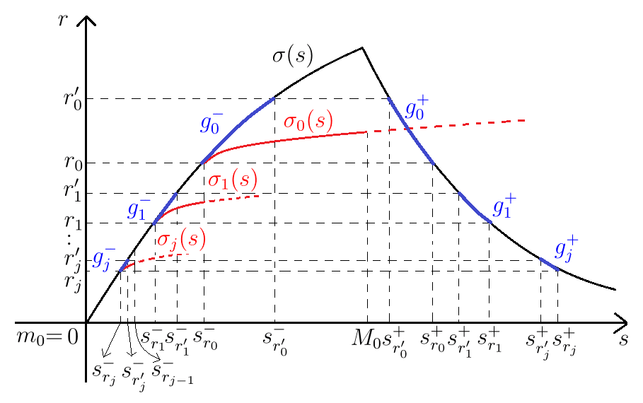
Figure 8. Iteration scheme for Case 1: $0=m_{0}<M_{0}$

By Theorem 3.1, there exists a solution $u^{(0)*}\in C^{2,1}(\bar{\Omega}\times[t_{0},\infty))$ to problem $(j=0)$

$$\left\{\begin{array}[]{ll}u^{(0)*}_{t}=(\sigma_{0}(u^{(0)*}_{x}))_{x}&\mbox{in $\Omega\times(t_{0},\infty)$,}\\ u^{(0)*}=u_{0}&\mbox{on $\Omega\times\{t=t_{0}\}$,}\\ u^{(0)*}_{x}=0&\mbox{on $\partial\Omega\times(t_{0},\infty)$,}\end{array}\right.$$

with $t_{0}:=0$, satisfying the properties in the statement of the theorem. By (3) and (4) of Theorem 3.1, we can choose the first time $t_{1}\in(t_{0},\infty)$ at which $\max_{\bar{\Omega}}u^{(0)*}_{x}(\cdot,t_{1})=s^{-}_{r_{0}}$. Also, from (3) of Theorem 3.1, it follows that $\min_{\bar{\Omega}}u^{(0)*}_{x}(\cdot,t)=0$ for all $t\in[t_{0},t_{1}]$. We define $u_{1}=u^{(0)*}(\cdot,t_{1})\in C^{2+\alpha}(\bar{\Omega})$ so that $u_{1}^{\prime}=0$ on $\partial\Omega$.

Again, by Theorem 3.1, there exists a solution $u^{(1)*}\in C^{2,1}(\bar{\Omega}\times[t_{1},\infty))$ to problem $(j=1)$

$$\left\{\begin{array}[]{ll}u^{(1)*}_{t}=(\sigma_{1}(u^{(1)*}_{x}))_{x}&\mbox{in $\Omega\times(t_{1},\infty)$,}\\ u^{(1)*}=u_{1}&\mbox{on $\Omega\times\{t=t_{1}\}$,}\\ u^{(1)*}_{x}=0&\mbox{on $\partial\Omega\times(t_{1},\infty)$,}\end{array}\right.$$

satisfying the properties in the statement of the theorem. By (3) and (4) of Theorem 3.1, we can choose the first time $t_{2}\in(t_{1},\infty)$ at which $\max_{\bar{\Omega}}u^{(1)*}_{x}(\cdot,t_{2})=s^{-}_{r_{1}}$. It also follows that $\min_{\bar{\Omega}}u^{(1)*}_{x}(\cdot,t)=0$ for all $t\in[t_{1},t_{2}]$. We define $u_{2}=u^{(1)*}(\cdot,t_{2})\in C^{2+\alpha}(\bar{\Omega})$ so that $u_{2}^{\prime}=0$ on $\partial\Omega$.

Repeating this process indefinitely, we obtain a sequence $0=t_{0}<t_{1}<t_{2}<\cdots<\infty$, a sequence $u_{j}\in C^{2+\alpha}(\bar{\Omega})$ with $u_{j}^{\prime}=0$ on $\partial\Omega$, and a sequence $u^{(j)*}\in C^{2+\alpha,1+\alpha/2}(\bar{\Omega}\times[t_{j},t_{j+1}])$ such that for each integer $j\geq 0$,

(6.4) $$\left\{\begin{array}[]{ll}\mbox{$u^{(j)*}_{t}=(\sigma_{j}(u^{(j)*}_{x}))_{x}$ in $\Omega\times(t_{j},t_{j+1})$,}\\ \mbox{$u^{(j)*}=u_{j}$ on $\Omega\times\{t=t_{j}\}$,}\\ \mbox{$u^{(j)*}=u_{j+1}$ on $\Omega\times\{t=t_{j+1}\}$,}\\ \mbox{$u^{(j)*}_{x}=0$ on $\partial\Omega\times(t_{j},t_{j+1})$,}\\ 0=\underset{\bar{\Omega}}{\min}u_{j}^{\prime}<\underset{\bar{\Omega}}{\max}u_{j}^{\prime}=\left\{\begin{array}[]{l}\mbox{$M_{0}$ if $j=0$,}\\ \mbox{$s^{-}_{r_{j-1}}$ if $j\geq 1$,}\end{array}\right.\\ \begin{split}0&=\min_{\bar{\Omega}}u^{(j)*}_{x}(\cdot,s)=\min_{\bar{\Omega}}u^{(j)*}_{x}(\cdot,t)\\ &<\max_{\bar{\Omega}}u^{(j)*}_{x}(\cdot,t)\leq\max_{\bar{\Omega}}u^{(j)*}_{x}(\cdot,s)\;\;\mbox{for all $t_{j}\leq s<t\leq t_{j+1}$.}\end{split}\end{array}\right.$$

We write $T=\underset{j\to\infty}{\lim}t_{j}\in(0,\infty]$.

Setup and subsolution in the $j^{th}$ step

We fix an index $j\geq 0$ here and below and carry out analysis on the $j^{th}$ step.

Let

$$\begin{split}g_{j}^{+}&=g^{+}_{r_{j},r_{j}^{\prime}}=(\sigma|_{[s^{+}_{r_{j}^{\prime}},s^{+}_{r_{j}}]})^{-1}:[r_{j},r_{j}^{\prime}]\to[s^{+}_{r_{j}^{\prime}},s^{+}_{r_{j}}],\\ g_{j}^{-}&=g^{-}_{r_{j},r_{j}^{\prime}}=(\sigma|_{[s^{-}_{r_{j}},s^{-}_{r_{j}^{\prime}}]})^{-1}:[r_{j},r_{j}^{\prime}]\to[s^{-}_{r_{j}},s^{-}_{r_{j}^{\prime}}];\end{split}$$

then $g_{j}^{-}\leq g_{j}^{-}(r_{j}^{\prime})=s^{-}_{r_{j}^{\prime}}<s^{+}_{r_{j}^{\prime}}=g_{j}^{+}(r_{j}^{\prime})\leq g_{j}^{+}$ on $[r_{j},r_{j}^{\prime}]$ (see Figure 8).

Define

$$Q_{j}=\big{\{}(x,t)\in\Omega\times(t_{j},t_{j+1})\,|\,s^{-}_{r_{j}}<u^{(j)*}_{x}(x,t)<s^{+}_{r_{j}}\big{\}};$$

then it follows from (6.4) that $\emptyset\neq\bar{Q}_{j}\subset\Omega\times[t_{j},t_{j+1}]$.

Let $b_{j}=\|u^{(j)*}_{t}\|_{L^{\infty}(Q_{j})}+1$. With the functions $g_{j}^{\pm}$ defined above, for each $u\in\mathbb{R}$, let $K_{b_{j}}(u)=K_{g_{j}^{+},g_{j}^{-};b_{j}}(u)$ and $U_{b_{j}}(u)=U_{g_{j}^{+},g_{j}^{-};b_{j}}(u)$ be defined as in Subsection 3.5. Define an auxiliary function $v^{(j)*}$ by

$$v^{(j)*}(x,t)=\int_{t_{j}}^{t}\sigma_{j}(u^{(j)*}_{x}(x,\tau))\,d\tau+\int_{0}^{x}u_{j}(y)\,dy\;\;\forall(x,t)\in\Omega\times(t_{j},t_{j+1});$$

then

(6.5) $$\left\{\begin{array}[]{l}v^{(j)*}_{t}=\sigma_{j}(u^{(j)*}_{x})\\ v^{(j)*}_{x}=u^{(j)*}\end{array}\right.\;\;\mbox{in $\Omega\times(t_{j},t_{j+1})$},$$

so that $w^{(j)*}:=(u^{(j)*},v^{(j)*})\in(C^{2,1}\times C^{3,1})(\bar{\Omega}\times[t_{j},t_{j+1}]).$ From this, (6.3) and the definition of $b_{j}$, it follows that

$$\nabla w^{(j)*}\in U_{b_{j}}(u^{(j)}_{*})\;\;\mbox{in $Q_{j}$;}$$

thus $w^{(j)*}|_{Q_{j}}$ is a strict subsolution of differential inclusion (3.3) with $Q=Q_{j}$, and so $0<\Gamma^{Q_{j}}_{w^{(j)*}}<1$, where the gauge operator $\Gamma^{Q_{j}}_{\cdot}=\Gamma^{Q_{j}}_{g_{j}^{+},g_{j}^{-};\cdot}$ is given as in Subsection 3.5.

Admissible class in the $j^{th}$ step

With $\epsilon=\min\{2^{-j},\Gamma^{Q_{j}}_{w^{(j)*}}\}$ and the above notation, let $\mathcal{A}_{j}=\mathcal{A}_{g_{j}^{+},g_{j}^{-},b_{j},w^{(j)*},Q_{j},\epsilon}$ and $\mathcal{A}_{j,\delta}=\mathcal{A}_{g_{j}^{+},g_{j}^{-},b_{j},w^{(j)*},Q_{j},\epsilon;\delta}$ $(\delta>0)$ be defined as in Subsection 3.5. We then define a class $\mathfrak{A}_{j}$ of admissible functions by

$$\mathfrak{A}_{j}=\left\{\begin{array}[]{l}w^{(j)}=(u^{(j)},v^{(j)})\in\\ (C^{2,1}\times C^{3,1})(\bar{\Omega}\times[t_{j},t_{j+1}])\end{array}\,\Big{|}\,\begin{array}[]{l}\mbox{$w^{(j)}=w^{(j)*}$ in}\\ \mbox{$(\Omega\times(t_{j},t_{j+1}))\setminus Q_{j}$,}\\ \mbox{$w^{(j)}|_{Q_{j}}\in\mathcal{A}_{j}$}\end{array}\right\};$$

then $w^{(j)*}\in\mathfrak{A}_{j},$ and so $\mathfrak{A}_{j}\neq\emptyset$. Also, for each $\delta>0,$ let $\mathfrak{A}_{j,\delta}$ be the subclass of functions $w^{(j)}\in\mathfrak{A}_{j}$ such that $w^{(j)}|_{Q_{j}}\in\mathcal{A}_{j,\delta}$.

Baire’s category method in the $j^{th}$ step

Let $\mathfrak{X}_{j}$ denote the closure of $\mathfrak{A}_{j}$ in the space $L^{\infty}(\Omega\times(t_{j},t_{j+1});\mathbb{R}^{2})$; then $(\mathfrak{X}_{j},L^{\infty})$ becomes a nonempty complete metric space. From the definition of $\mathfrak{A}_{j}$, it is easy to check that

$$\mathfrak{X}_{j}\subset w^{(j)*}+W^{1,\infty}_{0}(\Omega\times(t_{j},t_{j+1});\mathbb{R}^{2}).$$

As in the proof of Theorem 2.2, we also see that the set of points of continuity for the space-time gradient operator $\nabla_{j}=\nabla:\mathfrak{X}_{j}\to L^{1}(\Omega\times(t_{j},t_{j+1});\mathbb{M}^{2\times 2})$, say $\mathfrak{C}_{\nabla_{j}}$, is dense in $\mathfrak{X}_{j}$.

Solutions over $[t_{j},t_{j+1}]$ from $\mathfrak{C}_{\nabla_{j}}$

Let $w^{(j)}=(u^{(j)},v^{(j)})\in\mathfrak{C}_{\nabla_{j}}.$ From Lemma 3.5 and the density of $\mathfrak{A}_{j}$ in $\mathfrak{X}_{j}$, it follows that $\mathfrak{A}_{j,\frac{1}{k}}$ is dense in $\mathfrak{X}_{j}$ for each $k\in\mathbb{N}$. So we can take a sequence $w^{(j)}_{k}=(u^{(j)}_{k},v^{(j)}_{k})\in\mathfrak{A}_{j,\frac{1}{k}}$ such that $\|w^{(j)}_{k}-w^{(j)}\|_{L^{\infty}(\Omega\times(t_{j},t_{j+1}))}\to 0$ as $k\to\infty$. By the continuity of the operator $\nabla_{j}$ at $w^{(j)}$, we have $\nabla w^{(j)}_{k}\to\nabla w^{(j)}$ in $L^{1}(\Omega\times(t_{j},t_{j+1});\mathbb{M}^{2\times 2})$ and hence pointwise a.e. in $\Omega\times(t_{j},t_{j+1})$ after passing to a subsequence if necessary.

We now state some properties of the function $w^{(j)}_{k}=(u^{(j)}_{k},v^{(j)}_{k})$ inherited from its membership $w^{(j)}_{k}\in\mathfrak{A}_{j,\frac{1}{k}}$:

(6.6) $$\left\{\begin{array}[]{l}w^{(j)}_{k}=(u^{(j)}_{k},v^{(j)}_{k})\in(C^{2,1}\times C^{3,1})(\bar{\Omega}\times[t_{j},t_{j+1}]),\\ \mbox{$w^{(j)}_{k}=w^{(j)*}$ in $(\Omega\times(t_{j},t_{j+1}))\setminus\bar{Q}^{w^{(j)}_{k}}_{j}$ for some open set $Q^{w^{(j)}_{k}}_{j}\subset\subset Q_{j}$}\\ \mbox{\quad\quad with $|\partial Q^{w^{(j)}_{k}}_{j}|=0$,}\\ \|u^{(j)}_{k}-u^{(j)*}\|_{L^{\infty}(Q_{j})}<2^{-(j+1)},\;\|(u^{(j)}_{k})_{t}-u^{(j)*}_{t}\|_{L^{\infty}(Q_{j})}<2^{-(j+1)},\\ \quad\quad|\Gamma^{Q_{j}}_{w^{(j)}_{k}}-\Gamma^{Q_{j}}_{w^{(j)*}}|<\Gamma^{Q_{j}}_{w^{(j)*}}/2,\;\;\mbox{(by the choice of $\epsilon$ above)}\\ \mbox{$\nabla w^{(j)}_{k}\in U_{b_{j}}(u^{(j)}_{k})$ in $Q_{j}$, and}\\ \int_{Q_{j}}\mathrm{dist}\big{(}\nabla w^{(j)}_{k}(x,t),K_{b_{j}}(u^{(j)}_{k}(x,t))\big{)}\,dxdt\leq\frac{1}{k}|Q_{j}|.\end{array}\right.$$

Let $k\to\infty$ in (6.6); then we get

(6.7) $$\left\{\begin{array}[]{l}\mbox{$w^{(j)}=w^{(j)*}$ in $(\bar{\Omega}\times[t_{j},t_{j+1}])\setminus Q_{j}$,}\\ \mbox{$\nabla w^{(j)}=\nabla w^{(j)*}$ a.e. in $(\Omega\times(t_{j},t_{j+1}))\setminus Q_{j}$,}\\ \|u^{(j)}-u^{(j)*}\|_{L^{\infty}(Q_{j})}\leq 2^{-(j+1)},\\ \|u^{(j)}_{t}-u^{(j)*}_{t}\|_{L^{\infty}(Q_{j})}\leq 2^{-(j+1)},\\ |\Gamma^{Q_{j}}_{w^{(j)}}-\Gamma^{Q_{j}}_{w^{(j)*}}|\leq\Gamma^{Q_{j}}_{w^{(j)*}}/2,\\ \mbox{$\nabla w^{(j)}\in K_{b_{j}}(u^{(j)})$ a.e. in $Q_{j}$.}\end{array}\right.$$

The last part of this also implies that a.e. in $Q_{j}$,

(6.8) $$\left\{\begin{array}[]{l}v^{(j)}_{t}=\sigma(u^{(j)}_{x}),\\ u^{(j)}_{x}\in[s^{-}_{r_{j}},s^{-}_{r_{j}^{\prime}}]\cup[s^{+}_{r_{j}^{\prime}},s^{+}_{r_{j}}].\end{array}\right.$$

On the other hand, it follows from (6.4), (6.6) and the definition of $Q_{j}$ that $(v^{(j)}_{k})_{t}=v^{(j)*}_{t}$ and $(u^{(j)}_{k})_{x}=u^{(j)*}_{x}\in[0,s^{-}_{r_{j}}]$ in $(\Omega\times(t_{j},t_{j+1}))\setminus Q_{j}$. Here, let $k\to\infty$; then we have from (6.3) and (6.5) that a.e. in $(\Omega\times(t_{j},t_{j+1}))\setminus Q_{j}$,

(6.9) $$v^{(j)}_{t}=v^{(j)*}_{t}=\sigma_{j}(u^{(j)*}_{x})=\sigma(u^{(j)*}_{x})=\sigma(u^{(j)}_{x}).$$

Next, choose any $\zeta\in C^{\infty}(\bar{\Omega}\times[t_{j},t_{j+1}])$ and $\tau\in[t_{j},t_{j+1}]$. From (6.5) and (6.6), it follows as in the proof of Theorem 2.2 that

$$\begin{split}\int_{t_{j}}^{\tau}&\int_{0}^{L}u^{(j)}_{k}\zeta_{t}\,dxdt\\ =&\int_{t_{j}}^{\tau}\int_{0}^{L}(v^{(j)}_{k})_{t}\zeta_{x}\,dxdt-\int_{t_{j}}^{\tau}\big{(}v^{(j)*}_{t}(L,t)\zeta(L,t)-v^{(j)*}_{t}(0,t)\zeta(0,t)\big{)}\,dt\\ &+\int_{0}^{L}\big{(}u^{(j)}_{k}(x,\tau)\zeta(x,\tau)-u_{j}(x,t_{j})\zeta(x,t_{j})\big{)}\,dx.\end{split}$$

Let $k\to\infty$; then from (6.8), (6.9) and $v^{(j)*}_{t}=\sigma_{j}(u^{(j)*}_{x})=0$ on $\partial\Omega\times[t_{j},t_{j+1}]$, we have

(6.10) $$\begin{split}\int_{t_{j}}^{\tau}&\int_{0}^{L}u^{(j)}\zeta_{t}\,dxdt\\ &=\int_{t_{j}}^{\tau}\int_{0}^{L}v^{(j)}_{t}\zeta_{x}\,dxdt+\int_{0}^{L}\big{(}u^{(j)}(x,\tau)\zeta(x,\tau)-u_{j}(x,t_{j})\zeta(x,t_{j})\big{)}\,dx\\ &=\int_{t_{j}}^{\tau}\int_{0}^{L}\sigma(u^{(j)}_{x})\zeta_{x}\,dxdt+\int_{0}^{L}\big{(}u^{(j)}(x,\tau)\zeta(x,\tau)-u_{j}(x)\zeta(x,t_{j})\big{)}\,dx.\end{split}$$

Gauge estimate for $w^{(j)*}$

Observe from (6.3), (6.4) and the definition of $Q_{j}$ that for all $(x,t)\in Q_{j}$,

$$Z_{w^{(j)*}}(x,t)=\frac{u^{(j)*}_{x}(x,t)-g_{j}^{-}(v^{(j)*}_{t}(x,t))}{g_{j}^{+}(v^{(j)*}_{t}(x,t))-g_{j}^{-}(v^{(j)*}_{t}(x,t))}\leq\frac{s^{-}_{r_{j-1}}}{s^{+}_{r_{j}^{\prime}}-s^{-}_{r_{j}^{\prime}}}=:e_{j},$$

where $j\geq 1$ and $Z_{w^{(j)*}}=Z^{Q_{j}}_{g_{j}^{+},g_{j}^{-};w^{(j)*}}$ is as in Subsection 3.5. We thus have

(6.11) $$\Gamma^{Q_{j}}_{w^{(j)*}}=\frac{1}{|Q_{j}|}\int_{Q_{j}}Z_{w^{(j)*}}(x,t)\,dxdt\leq e_{j}\;\;(j\geq 1).$$

Note also that $\underset{j\to\infty}{\lim}e_{j}=0$.

Blow-up estimate in the $j^{th}$ step

From (6.11), it follows that $0<\Gamma^{Q_{j}}_{w^{(j)*}}\leq e_{j}\to 0$ as $j\to\infty;$ so there exists an index $j_{0}\geq 0$ such that $0<\Gamma^{Q_{j}}_{w^{(j)*}}<1/2$ for all integers $j\geq j_{0}$, and so $0<\Gamma^{Q_{j}}_{w^{(j)}}<1$ for all $j\geq j_{0}$ by the fifth of (6.7). Thus, for all $j\geq j_{0}$, we have

$$\left\{\begin{array}[]{l}|Q^{+}_{j}|:=\big{|}\big{\{}(x,t)\in Q_{j}\,|\,u^{(j)}_{x}(x,t)\in[s^{+}_{r_{j}^{\prime}},s^{+}_{r_{j}}]\big{\}}\big{|}>0,\\ |Q^{-}_{j}|:=\big{|}\big{\{}(x,t)\in Q_{j}\,|\,u^{(j)}_{x}(x,t)\in[s^{-}_{r_{j}},s^{-}_{r_{j}^{\prime}}]\big{\}}\big{|}>0.\end{array}\right.$$

From this, we have

(6.12) $$\|u^{(j)}_{x}\|_{L^{\infty}(\Omega\times(t_{j},t_{j+1}))}\geq s^{+}_{r^{\prime}_{j}}\;\;\forall j\geq j_{0}.$$

Note also that $\underset{j\to\infty}{\lim}s^{+}_{r^{\prime}_{j}}=\infty$.

Energy estimate in the $j^{th}$ step

We now consider the quantity

$$\begin{split}\frac{1}{t_{j+1}-t_{j}}&\int_{t_{j}}^{t_{j+1}}\mathcal{E}(u^{(j)}(\cdot,t))\,dt=\frac{1}{t_{j+1}-t_{j}}\int_{t_{j}}^{t_{j+1}}\int_{\Omega}W(u^{(j)}_{x}(x,t))\,dxdt\\ =&\frac{1}{t_{j+1}-t_{j}}\Big{(}\int_{Q^{+}_{j}}+\int_{Q^{-}_{j}}+\int_{(\Omega\times(t_{j},t_{j+1}))\setminus Q_{j}}\Big{)}W(u^{(j)}_{x})=:I_{1}^{+}+I_{1}^{-}+I_{2}.\end{split}$$

From the fifth of (6.7), (6.8), (6.11) and the definition of $\Gamma^{Q_{j}}_{\cdot}$, we have

$$\frac{|Q_{j}^{+}|}{|Q_{j}|}=\Gamma^{Q_{j}}_{w^{(j)}}\leq\frac{3}{2}\Gamma^{Q_{j}}_{w^{(j)*}}\leq\frac{3e_{j}}{2}\;\;(j\geq 1).$$

By the hypotheses on the diffusion flux $\sigma$ of the Perona-Malik type, there exists a number $c_{0}>0$ such that $0\leq W(s)\leq|s|$ for all $s\in\mathbb{R}$ with $|s|\geq c_{0}.$ Thus it follows from the definition of $Q^{+}_{j}$ and $e_{j}$ that for all sufficiently large $j\geq 1$,

$$I_{1}^{+}\leq\frac{1}{t_{j+1}-t_{j}}\int_{Q^{+}_{j}}u_{x}^{(j)}\,dxdt\leq\frac{s^{+}_{r_{j}}|Q^{+}_{j}|}{t_{j+1}-t_{j}}\leq\frac{3e_{j}s^{+}_{r_{j}}|Q_{j}|}{2(t_{j+1}-t_{j})}\leq\frac{3Ls^{+}_{r_{j}}s^{-}_{r_{j-1}}}{2(s^{+}_{r_{j}^{\prime}}-s^{-}_{r_{j}^{\prime}})}.$$

Also, we easily have from (6.4), the second of (6.7) and the definition of $Q^{-}_{j}$ that

$$I^{-}_{1}+I_{2}\leq\frac{W(s^{-}_{r_{j}^{\prime}})|\Omega\times(t_{j},t_{j+1})|}{t_{j+1}-t_{j}}=LW(s^{-}_{r_{j}^{\prime}}).$$

Combining these estimates, for all sufficiently large $j\geq 1$, we get

(6.13) $$\frac{1}{t_{j+1}-t_{j}}\int_{t_{j}}^{t_{j+1}}\mathcal{E}(u^{(j)}(\cdot,t))\,dt\leq\frac{3Ls^{+}_{r_{j}}s^{-}_{r_{j-1}}}{2(s^{+}_{r_{j}^{\prime}}-s^{-}_{r_{j}^{\prime}})}+LW(s^{-}_{r_{j}^{\prime}})=:d_{j}.$$

Note also from (6.2) that $\underset{j\to\infty}{\lim}d_{j}=0$.

Stability in the $j^{th}$ step

Recall the Poincaré inequality in 1-D: there exists a constant $C>0$, depending only on $\Omega=(0,L)$, such that

$$\|f-\bar{f}\|_{\infty}\leq C\|f^{\prime}\|_{\infty}\;\;\forall f\in W^{1,\infty}(\Omega),$$

where $\bar{f}:=\frac{1}{L}\int_{0}^{L}f(x)\,dx$. Using this, it follows from (6.4) that for all $t\in[t_{j},t_{j+1}]$,

$$\|u^{(j)*}(\cdot,t)-\bar{u}_{0}\|_{\infty}\leq C\|u^{(j)*}_{x}(\cdot,t)\|_{\infty}\leq Cs^{-}_{r_{j-1}}\;\;(j\geq 1);$$

thus by the first and third of (6.7), for all $t\in[t_{j},t_{j+1}]$,

(6.14) $$\|u^{(j)}(\cdot,t)-\bar{u}_{0}\|_{\infty}\leq Cs^{-}_{r_{j-1}}+2^{-(j+1)}\;\;(j\geq 1).$$

Solutions by patching

In this final step, we show that the set

$$\mathcal{S}:=\Bigg{\{}u=\sum_{j=0}^{\infty}u^{(j)}\chi_{\bar{\Omega}\times[t_{j},t_{j+1})}\,\Big{|}\,w^{(j)}=(u^{(j)},v^{(j)})\in\mathfrak{C}_{\nabla_{j}}\;\;\forall j\geq 0\Bigg{\}}$$

consists of infinitely many weak solutions $u$ to problem (1.1) satisfying (1)–(4).

Firstly, we check that $\mathcal{S}$ is an infinite set. For each $j\geq 0$, we can see as in the proof of Theorem 2.2 that $\mathfrak{C}_{\nabla_{j}}$ is an infinite set and that for $w^{(j)}_{1}=(u^{(j)}_{1},v^{(j)}_{1}),w^{(j)}_{2}=(u^{(j)}_{2},v^{(j)}_{2})\in\mathfrak{C}_{\nabla_{j}}$, we have $w^{(j)}_{1}=w^{(j)}_{2}\Longleftrightarrow u^{(j)}_{1}=u^{(j)}_{2}$. Thus $\mathcal{S}$ must be an infinite set.

Secondly, we construct a suitable open set $G$ in $\mathbb{R}^{2}$ with $\partial\Omega\times[0,T)\subset G$. By definition, we know that $\bar{Q}_{j}$ is a nonempty compact subset of $\Omega\times[t_{j},t_{j+1}]$ for each $j\geq 0$. So $F:=\underset{j\geq 0}{\bigcup}\bar{Q}_{j}$ is closed in $\mathbb{R}\times(-\infty,T)$. Let $G=(\mathbb{R}\times(-\infty,T))\setminus F;$ then $G$ is open in $\mathbb{R}^{2}$, and $\partial\Omega\times[0,T)\subset G.$

Choose any $u\in\mathcal{S}$ so that

$$u=\sum_{j=0}^{\infty}u^{(j)}\chi_{\bar{\Omega}\times[t_{j},t_{j+1})}$$

for some sequence $w^{(j)}=(u^{(j)},v^{(j)})\in\mathfrak{C}_{\nabla_{j}}$ $(j\geq 0)$. Finally, we verify that $u$ is a weak solution to problem (1.1) fulfilling (1)–(4).

To prove (1), it is equivalent to show that $u\in C^{2+\alpha,1+\alpha/2}(\overline{G\cap\Omega_{t_{j}}})$ for all $j\in\mathbb{N}$. We proceed it by induction on $j\in\mathbb{N}$. First, note from the first of (6.7) that

$$u=u^{(0)}=u^{(0)*}\in C^{2+\alpha,1+\alpha/2}\big{(}\overline{(\Omega\times(0,t_{1}))\setminus\bar{Q}_{0}}\big{)}=C^{2+\alpha,1+\alpha/2}(\overline{G\cap\Omega_{t_{1}}});$$

so the inclusion holds for $j=1$. Next, assume that the inclusion is valid for $j=m\in\mathbb{N}$. Note that $(\bar{Q}_{m-1}\cup\bar{Q}_{m})\cap(\Omega\times\{t=t_{m}\})$ is a compact subset of $\Omega\times\{t=t_{m}\}$. Fix any point $x_{0}\in\Omega$ such that $(x_{0},t_{m})\not\in\bar{Q}_{m-1}\cup\bar{Q}_{m}.$ Then choose an open rectangle $B$ in $\mathbb{R}^{2}$ with center $(x_{0},t_{m})$, parallel to the axes, so small that its closure $\bar{B}$ does not intersect with $\bar{Q}_{m-1}\cup\bar{Q}_{m}$, $\Omega\times\{t=t_{m\pm 1}\}$ and $\partial\Omega\times[t_{m-1},t_{m+1}]$. Let us write

$$\begin{split}B^{+}&=\{(x,t)\in B\,|\,t>t_{m}\},\\ B^{-}&=\{(x,t)\in B\,|\,t<t_{m}\},\\ B^{0}&=\{(x,t)\in B\,|\,t=t_{m}\}.\end{split}$$

We then have from the first of (6.7) that $u=u^{(m-1)*}\in C^{2+\alpha,1+\alpha/2}(\bar{B}^{-})$ and $u=u^{(m)*}\in C^{2+\alpha,1+\alpha/2}(\bar{B}^{+})$. Also, by (6.4), $u^{(m-1)*}$ and $u^{(m)*}$ are both equal to the function $u_{m}=u_{m}(x)$ on $\Omega\times\{t=t_{m}\},$ where $0\leq u_{m}^{\prime}\leq s^{-}_{r_{m}}$ on $\bar{B}^{0}$ by the definition of $Q_{m}$. From (6.3), we have $\sigma_{m-1}=\sigma=\sigma_{m}$ on $[0,s^{-}_{r_{m}}]$; thus, with the help of (6.4), we get $u\in C^{2+\alpha,1+\alpha/2}(\bar{B})$. On the other hand, also from the first of (6.7), we have $u=u^{(m)*}\in C^{2+\alpha,1+\alpha/2}\big{(}\overline{(\Omega\times(t_{m},t_{m+1}))\setminus\bar{Q}_{m}}\big{)}$. Using the induction hypothesis, we can now conclude that $u\in C^{2+\alpha,1+\alpha/2}(\overline{G\cap\Omega_{t_{m+1}}})$. Therefore, (1) holds.

Note that (2), (3) and (4) follow immediately from (6.14), (6.12) and (6.13), respectively. It is also a simple consequence of (6.10) by patching that $u$ is a weak solution to problem (1.1).

The proof of Case 1: $0=m_{0}<M_{0}$ is now complete.

6.2. Case 3: $m_{0}<0<M_{0}$

We now focus on the proof of Case 3: $m_{0}<0<M_{0}$, which requires a careful hierarchical iteration process.

Setup for iteration hierarchy

We describe an iteration scheme that shows a hierarchical pattern. In each of the steps of iteration, we encounter four possible outcomes among which the two make us stop the iteration and apply either the result of Case 1 or that of Case 2 to complete the proof. The other two possible outcomes keep us going further to the next step of iteration.

$0^{th}$ step of hierarchy

Let $\max\{\sigma(s_{1}),-1\}<r_{1,0}<0<r_{2,0}<\min\{\sigma(s_{2}),1\}$ be any two numbers such that

$$s^{-}_{r_{1,0}}<m_{0}<s^{+}_{r_{1,0}}<0<s^{-}_{r_{2,0}}<M_{0}<s^{+}_{r_{2,0}},$$

and let $r^{\prime}_{1,0}\in(\sigma(s_{1}),r_{1,0})$, $r^{\prime}_{2,0}\in(r_{2,0},\sigma(s_{2}))$ be close enough to $r_{1,0}$, $r_{2,0}$, respectively, so that

$$s^{-}_{r_{1,0}^{\prime}}-s^{-}_{r_{1,0}}<1\;\;\mbox{and}\;\;s^{+}_{r_{2,0}}-s^{+}_{r_{2,0}^{\prime}}<1.$$

Then choose a function $\sigma_{0}\in C^{3}(\mathbb{R})$ such that

$$\left\{\begin{array}[]{l}\mbox{$\sigma_{0}=\sigma$ on $[s^{+}_{r_{1,0}},s^{-}_{r_{2,0}}]$,}\\ \mbox{$\sigma_{0}>\max\{\sigma,r^{\prime}_{1,0}\}$ on $[m_{0},s^{+}_{r_{1,0}})$,}\\ \mbox{$\sigma_{0}<\min\{\sigma,r^{\prime}_{2,0}\}$ on $(s^{-}_{r_{2,0}},M_{0}]$,}\\ \mbox{$\sigma_{0}^{\prime}>0$ in $\mathbb{R}$}.\end{array}\right.$$

By Theorem 3.1, we have a solution $u^{(0)*}\in C^{2,1}(\bar{\Omega}\times[t_{0},\infty))$ to problem

$$\left\{\begin{array}[]{ll}u^{(0)*}_{t}=(\sigma_{0}(u^{(0)*}_{x}))_{x}&\mbox{in $\Omega\times(t_{0},\infty)$,}\\ u^{(0)*}=u_{0}&\mbox{on $\Omega\times\{t=t_{0}\}$,}\\ u^{(0)*}_{x}=0&\mbox{on $\partial\Omega\times(t_{0},\infty)$,}\end{array}\right.$$

with $t_{0}:=0$, satisfying the properties in the statement of the theorem. By (3) and (4) of Theorem 3.1, we can choose the first time $t_{1,1}\in(t_{0},\infty)$ at which $\min_{\bar{\Omega}}u^{(0)*}_{x}(\cdot,t_{1,1})=s^{+}_{r_{1,0}}$ and the first time $t_{2,1}\in(t_{0},\infty)$ at which $\max_{\bar{\Omega}}u^{(0)*}_{x}(\cdot,t_{2,1})=s^{-}_{r_{2,0}}$.

We now have $t_{2,1}\leq t_{1,1}$ or $t_{1,1}\leq t_{2,1}$. First, assume $t_{2,1}\leq t_{1,1}$; then we have the dichotomy:

$$m_{1,1}:=\max_{\bar{\Omega}}u^{(0)*}_{x}(\cdot,t_{1,1})=0\;\;\mbox{or}\;\;m_{1,1}>0.$$

In any case, we have $m_{1,1}\leq s^{-}_{r_{2,0}}$ by (3) of Theorem 3.1.

Second, assume $t_{1,1}\leq t_{2,1}$; then we have the dichotomy:

$$m_{2,1}:=\min_{\bar{\Omega}}u^{(0)*}_{x}(\cdot,t_{2,1})=0\;\;\mbox{or}\;\;m_{2,1}<0.$$

Likewise, we have $m_{2,1}\geq s^{+}_{r_{1,0}}$.

Here and below, without any ambiguity, whenever $m_{1,1}$ appears in the context, it will be understood that we assume $t_{2,1}\leq t_{1,1}$ in advance, and the same also applies to the case of $m_{2,1}$ with $t_{1,1}\leq t_{2,1}$.

In the case that $m_{1,1}=0$ or that $m_{2,1}=0$, we stop the hierarchical iteration. In the case that $m_{1,1}>0$ or that $m_{2,1}<0$, we continue to the next step of iteration hierarchy as below.

$1^{st}$ step of hierarchy

Assume $m_{1,1}>0$ or $m_{2,1}<0$. In the case that $m_{1,1}>0$, we set $t_{1}=t_{1,1}$. If $m_{2,1}<0$, then we take $t_{1}=t_{2,1}$. In both cases, we then let $u_{1}=u^{(0)*}(\cdot,t_{1})\in C^{2+\alpha}(\bar{\Omega})$ so that $u_{1}^{\prime}=0$ on $\partial\Omega$.

First, assume $m_{1,1}>0$. Since $m_{1,1}\leq s^{-}_{r_{2,0}}$, we have $0<\sigma(m_{1,1})\leq r_{2,0}$. Now, let $\max\{r_{1,0},-2^{-1}\}<r_{1,1}<0<r_{2,1}<\min\{\sigma(m_{1,1}),2^{-1}\}$ be any two numbers.

Second, assume $m_{2,1}<0$. Since $m_{2,1}\geq s^{+}_{r_{1,0}}$, we have $0>\sigma(m_{2,1})\geq r_{1,0}$. Here, let $\max\{\sigma(m_{2,1}),-2^{-1}\}<r_{1,1}<0<r_{2,1}<\min\{r_{2,0},2^{-1}\}$ be any two numbers.

In both cases, let $r^{\prime}_{1,1}\in(r_{1,0},r_{1,1})$, $r^{\prime}_{2,1}\in(r_{2,1},r_{2,0})$ be close enough to $r_{1,1}$, $r_{2,1}$, respectively, so that

$$s^{-}_{r_{1,1}^{\prime}}-s^{-}_{r_{1,1}}<2^{-1}\;\;\mbox{and}\;\;s^{+}_{r_{2,1}}-s^{+}_{r_{2,1}^{\prime}}<2^{-1}.$$

Then choose a function $\sigma_{1}\in C^{3}(\mathbb{R})$ such that

$$\left\{\begin{array}[]{l}\mbox{$\sigma_{1}=\sigma$ on $[s^{+}_{r_{1,1}},s^{-}_{r_{2,1}}]$,}\\ \mbox{$\sigma_{1}>\max\{\sigma,r^{\prime}_{1,1}\}$ on $[s^{+}_{r_{1,0}},s^{+}_{r_{1,1}})$,}\\ \mbox{$\sigma_{1}<\min\{\sigma,r^{\prime}_{2,1}\}$ on $(s^{-}_{r_{2,1}},s^{-}_{r_{2,0}}]$,}\\ \mbox{$\sigma_{1}^{\prime}>0$ in $\mathbb{R}$}.\end{array}\right.$$

By Theorem 3.1, we have a solution $u^{(1)*}\in C^{2,1}(\bar{\Omega}\times[t_{1},\infty))$ to problem

$$\left\{\begin{array}[]{ll}u^{(1)*}_{t}=(\sigma_{1}(u^{(1)*}_{x}))_{x}&\mbox{in $\Omega\times(t_{1},\infty)$,}\\ u^{(1)*}=u_{1}&\mbox{on $\Omega\times\{t=t_{1}\}$,}\\ u^{(1)*}_{x}=0&\mbox{on $\partial\Omega\times(t_{1},\infty)$,}\end{array}\right.$$

satisfying the properties in the statement of the theorem. By (3) and (4) of Theorem 3.1, we can choose the first time $t_{1,2}\in(t_{1},\infty)$ at which $\min_{\bar{\Omega}}u^{(1)*}_{x}(\cdot,t_{1,2})=s^{+}_{r_{1,1}}$ and the first time $t_{2,2}\in(t_{1},\infty)$ at which $\max_{\bar{\Omega}}u^{(1)*}_{x}(\cdot,t_{2,2})=s^{-}_{r_{2,1}}$.

We now have $t_{2,2}\leq t_{1,2}$ or $t_{1,2}\leq t_{2,2}$. First, assume $t_{2,2}\leq t_{1,2}$; then we have the dichotomy:

$$m_{1,2}:=\max_{\bar{\Omega}}u^{(1)*}_{x}(\cdot,t_{1,2})=0\;\;\mbox{or}\;\;m_{1,2}>0.$$

Note from (3) of Theorem 3.1 that $m_{1,2}\leq s^{-}_{r_{2,1}}$.

Second, assume $t_{1,2}\leq t_{2,2}$; then we have the dichotomy:

$$m_{2,2}:=\min_{\bar{\Omega}}u^{(1)*}_{x}(\cdot,t_{2,2})=0\;\;\mbox{or}\;\;m_{2,2}<0.$$

Likewise, we have $m_{2,2}\geq s^{+}_{r_{1,1}}$.

Here and below, as in the $0^{th}$ step of hierarchy, whenever $m_{1,2}$ appears in the context, it will be understood that we assume $t_{2,2}\leq t_{1,2}$ in advance, and the same also applies to the case of $m_{2,2}$ with $t_{1,2}\leq t_{2,2}$.

In the case that $m_{1,2}=0$ or that $m_{2,2}=0$, we stop the hierarchical iteration. In the case that $m_{1,2}>0$ or that $m_{2,2}<0$, we continue to the next step of iteration hierarchy.

For a better understanding, we remark that, up to the $1^{st}$ step of hierarchy, we have $2^{1+1}=4$ possible hierarchical scenarios of length 2: $(m_{1,1},m_{1,2})$, $(m_{1,1},m_{2,2})$, $(m_{2,1},m_{1,2})$ and $(m_{2,1},m_{2,2})$. In each of these cases, the second component depends on the first one; for instance, the $m_{1,2}$ in $(m_{1,1},m_{1,2})$ and $(m_{2,1},m_{1,2})$ are not necessarily equal. Also, if and only if the second component of a hierarchical scenario of length 2 is nonzero, we continue to the $2^{nd}$ step of hierarchy; otherwise, we stop here.

$j^{th}$ step of hierarchy

Assume that we are given a hierarchical scenario $(m_{a_{1},1},\cdots,m_{a_{j},j})$ of length $j\geq 1$ whose each component is nonzero, where $a_{1},\cdots,a_{j}\in\{1,2\}$. In the case that $m_{a_{j},j}=m_{1,j}>0$, we set $t_{j}=t_{1,j}$. If $m_{a_{j},j}=m_{2,j}<0$, then we take $t_{j}=t_{2,j}$. In both cases, we then set $u_{j}=u^{(j-1)*}(\cdot,t_{j})\in C^{2+\alpha}(\bar{\Omega})$ so that $u_{j}^{\prime}=0$ on $\partial\Omega$.

First, assume $m_{a_{j},j}=m_{1,j}>0$. Since $m_{1,j}\leq s^{-}_{r_{2,j-1}}$, we have $0<\sigma(m_{1,j})\leq r_{2,j-1}$. Now, let $r_{1,j}$ and $r_{2,j}$ be any two numbers with

$$\max\{r_{1,j-1},-2^{-j}\}<r_{1,j}<0<r_{2,j}<\min\{\sigma(m_{1,j}),2^{-j}\}.$$

Second, assume $m_{a_{j},j}=m_{2,j}<0$. Since $m_{2,j}\geq s^{+}_{r_{1,j-1}}$, we have $0>\sigma(m_{2,j})\geq r_{1,j-1}$. Here, let $r_{1,j}$ and $r_{2,j}$ be any two numbers with

$$\max\{\sigma(m_{2,j}),-2^{-j}\}<r_{1,j}<0<r_{2,j}<\min\{r_{2,j-1},2^{-j}\}.$$

In both cases, let $r^{\prime}_{1,j}\in(r_{1,j-1},r_{1,j})$, $r^{\prime}_{2,j}\in(r_{2,j},r_{2,j-1})$ be close enough to $r_{1,j}$, $r_{2,j}$, respectively, so that

$$s^{-}_{r_{1,j}^{\prime}}-s^{-}_{r_{1,j}}<2^{-j}\;\;\mbox{and}\;\;s^{+}_{r_{2,j}}-s^{+}_{r_{2,j}^{\prime}}<2^{-j}.$$

Then choose a function $\sigma_{j}\in C^{3}(\mathbb{R})$ such that

$$\left\{\begin{array}[]{l}\mbox{$\sigma_{j}=\sigma$ on $[s^{+}_{r_{1,j}},s^{-}_{r_{2,j}}]$,}\\ \mbox{$\sigma_{j}>\max\{\sigma,r^{\prime}_{1,j}\}$ on $[s^{+}_{r_{1,j-1}},s^{+}_{r_{1,j}})$,}\\ \mbox{$\sigma_{j}<\min\{\sigma,r^{\prime}_{2,j}\}$ on $(s^{-}_{r_{2,j}},s^{-}_{r_{2,j-1}}]$,}\\ \mbox{$\sigma_{j}^{\prime}>0$ in $\mathbb{R}$}.\end{array}\right.$$

By Theorem 3.1, we have a solution $u^{(j)*}\in C^{2,1}(\bar{\Omega}\times[t_{j},\infty))$ to problem

$$\left\{\begin{array}[]{ll}u^{(j)*}_{t}=(\sigma_{j}(u^{(j)*}_{x}))_{x}&\mbox{in $\Omega\times(t_{j},\infty)$,}\\ u^{(j)*}=u_{j}&\mbox{on $\Omega\times\{t=t_{j}\}$,}\\ u^{(j)*}_{x}=0&\mbox{on $\partial\Omega\times(t_{j},\infty)$,}\end{array}\right.$$

satisfying the properties in the statement of the theorem. By (3) and (4) of Theorem 3.1, we can choose the first time $t_{1,j+1}\in(t_{j},\infty)$ at which $\min_{\bar{\Omega}}u^{(j)*}_{x}(\cdot,t_{1,j+1})=s^{+}_{r_{1,j}}$ and the first time $t_{2,j+1}\in(t_{j},\infty)$ at which $\max_{\bar{\Omega}}u^{(j)*}_{x}(\cdot,t_{2,j+1})=s^{-}_{r_{2,j}}$.

We now have $t_{2,j+1}\leq t_{1,j+1}$ or $t_{1,j+1}\leq t_{2,j+1}$. First, assume $t_{2,j+1}\leq t_{1,j+1}$; then we have the dichotomy:

$$m_{1,j+1}:=\max_{\bar{\Omega}}u^{(j)*}_{x}(\cdot,t_{1,j+1})=0\;\;\mbox{or}\;\;m_{1,j+1}>0.$$

Note $m_{1,j+1}\leq s^{-}_{r_{2,j}}$.

Second, assume $t_{1,j+1}\leq t_{2,j+1}$; then we have the dichotomy:

$$m_{2,j+1}:=\min_{\bar{\Omega}}u^{(j)*}_{x}(\cdot,t_{2,j+1})=0\;\;\mbox{or}\;\;m_{2,j+1}<0.$$

Note $m_{2,j+1}\geq s^{+}_{r_{1,j}}$.

Here and below, as in the previous steps of hierarchy, whenever $m_{1,j+1}$ appears in the context, it will be understood that we assume $t_{2,j+1}\leq t_{1,j+1}$ in advance, and the same also applies to the case of $m_{2,j+1}$ with $t_{1,j+1}\leq t_{2,j+1}$.

In the case that $m_{1,j+1}=0$ or that $m_{2,j+1}=0$, we stop the hierarchical iteration. In the case that $m_{1,j+1}>0$ or that $m_{2,j+1}<0$, we continue to the next step of iteration hierarchy.

Case of an infinite hierarchical scenario

We first finish the proof of Case 3 for the case of an infinite hierarchical scenario $(m_{a_{1},1},m_{a_{2},2},\cdots)$ with $a_{j}\in\{1,2\}$ and $m_{a_{j},j}\neq 0$ for all $j\in\mathbb{N}$.

By our setup for iteration hierarchy, for each integer $j\geq 0$, we have the following: with $r_{1,-1}:=\sigma(s_{1})$ and $r_{2,-1}:=\sigma(s_{2})$,

$$\left\{\begin{array}[]{l}\max\{r_{1,j-1},-2^{-j}\}<r_{1,j}<0<r_{2,j}<\min\{r_{2,j-1},2^{-j}\},\\ \left\{\begin{array}[]{l}\mbox{$r_{2,j}<\sigma(m_{1,j})$ if $j\geq 1$ and $a_{j}=1$,}\\ \mbox{$r_{1,j}>\sigma(m_{2,j})$ if $j\geq 1$ and $a_{j}=2$,}\end{array}\right.\\ \mbox{$r_{1,j-1}<r^{\prime}_{1,j}<r_{1,j}$, $r_{2,j}<r^{\prime}_{2,j}<r_{2,j-1}$,}\\ \mbox{$s^{-}_{r^{\prime}_{1,j}}-s^{-}_{r_{1,j}}<2^{-j}$, $s^{+}_{r_{2,j}}-s^{+}_{r^{\prime}_{2,j}}<2^{-j}$,}\\ \mbox{$\sigma_{j}\in C^{3}(\mathbb{R})$, $\sigma^{\prime}_{j}>0$ in $\mathbb{R}$,}\\ \mbox{$\sigma_{j}=\sigma$ on $[s^{+}_{r_{1,j}},s^{-}_{r_{2,j}}]$,}\\ \mbox{$\sigma_{j}>\max\{\sigma,r^{\prime}_{1,j}\}$ on $\left\{\begin{array}[]{l}\mbox{$[m_{0},s^{+}_{r_{1,0}})$ if $j=0,$}\\ \mbox{$[s^{+}_{r_{1,j-1}},s^{+}_{r_{1,j}})$ if $j\geq 1,$}\end{array}\right.$}\\ \mbox{$\sigma_{j}<\min\{\sigma,r^{\prime}_{2,j}\}$ on $\left\{\begin{array}[]{l}\mbox{$(s^{-}_{r_{2,0}},M_{0}]$ if $j=0,$}\\ \mbox{$(s^{-}_{r_{2,j}},s^{-}_{r_{2,j-1}}]$ if $j\geq 1,$}\end{array}\right.$}\end{array}\right.$$

$$\left\{\begin{array}[]{l}u^{(j)*}\in C^{2+\alpha,1+\alpha/2}(\bar{\Omega}\times[t_{j},t_{j+1}]),\\ \mbox{$u^{(j)*}_{t}=(\sigma_{j}(u^{(j)*}_{x}))_{x}$ in $\Omega\times(t_{j},t_{j+1})$,}\\ \mbox{$u^{(j)*}=u_{j}$ on $\Omega\times\{t=t_{j}\}$,}\\ \mbox{$u^{(j)*}=u_{j+1}$ on $\Omega\times\{t=t_{j+1}\}$,}\end{array}\right.$$

and

$$\left\{\begin{array}[]{l}0<\underset{\bar{\Omega}}{\max}u^{\prime}_{j}=\left\{\begin{array}[]{l}\mbox{$M_{0}$ if $j=0$,}\\ \mbox{$m_{1,j}$ if $j\geq 1$ and $a_{j}=1$, where $0<m_{1,j}\leq s^{-}_{r_{2,j-1}}$,}\\ \mbox{$s^{-}_{r_{2,j-1}}$ if $j\geq 1$ and $a_{j}=2$,}\end{array}\right.\\ 0>\underset{\bar{\Omega}}{\min}u^{\prime}_{j}=\left\{\begin{array}[]{l}\mbox{$m_{0}$ if $j=0$,}\\ \mbox{$s^{+}_{r_{1,j-1}}$ if $j\geq 1$ and $a_{j}=1$,}\\ \mbox{$m_{2,j}$ if $j\geq 1$ and $a_{j}=2$, where $0>m_{2,j}\geq s^{+}_{r_{1,j-1}}$,}\end{array}\right.\\ \mbox{$\underset{\bar{\Omega}}{\min}u^{(j)*}_{x}(\cdot,s)\leq\underset{\bar{\Omega}}{\min}u^{(j)*}_{x}(\cdot,t)<0$}\\ \mbox{$\;\;\,<\underset{\bar{\Omega}}{\max}u^{(j)*}_{x}(\cdot,t)\leq\underset{\bar{\Omega}}{\max}u^{(j)*}_{x}(\cdot,s)$ for all $t_{j}\leq s<t\leq t_{j+1}$.}\end{array}\right.$$

Note also that $0=t_{0}<t_{1}=t_{a_{1},1}<t_{2}=t_{a_{2},2}<\cdots$. We write $T=\underset{j\to\infty}{\lim}t_{j}\in(0,\infty]$.

We now fix an index $j\geq 0$ here and below and setup the $j^{th}$ step in a way similar to the proof of Case 1. Due to the similarity, we only sketch some parts that are different from that of Case 1.

Let

$$\begin{split}g^{+}_{1,j}&=g^{+}_{r_{1,j}^{\prime},r_{1,j}}=(\sigma|_{[s^{+}_{r_{1,j}^{\prime}},s^{+}_{r_{1,j}}]})^{-1}:[r_{1,j}^{\prime},r_{1,j}]\to[s^{+}_{r_{1,j}^{\prime}},s^{+}_{r_{1,j}}],\\ g^{-}_{1,j}&=g^{-}_{r_{1,j}^{\prime},r_{1,j}}=(\sigma|_{[s^{-}_{r_{1,j}},s^{-}_{r_{1,j}^{\prime}}]})^{-1}:[r_{1,j}^{\prime},r_{1,j}]\to[s^{-}_{r_{1,j}},s^{-}_{r_{1,j}^{\prime}}],\\ g^{+}_{2,j}&=g^{+}_{r_{2,j},r_{2,j}^{\prime}}=(\sigma|_{[s^{+}_{r_{2,j}^{\prime}},s^{+}_{r_{2,j}}]})^{-1}:[r_{2,j},r_{2,j}^{\prime}]\to[s^{+}_{r_{2,j}^{\prime}},s^{+}_{r_{2,j}}],\\ g^{-}_{2,j}&=g^{-}_{r_{2,j},r_{2,j}^{\prime}}=(\sigma|_{[s^{-}_{r_{2,j}},s^{-}_{r_{2,j}^{\prime}}]})^{-1}:[r_{2,j},r_{2,j}^{\prime}]\to[s^{-}_{r_{2,j}},s^{-}_{r_{2,j}^{\prime}}].\end{split}$$

Define

$$Q_{i,j}=\big{\{}(x,t)\in\Omega\times(t_{j},t_{j+1})\,|\,s^{-}_{r_{i,j}}<u^{(j)*}_{x}(x,t)<s^{+}_{r_{i,j}}\big{\}}\;\;(i=1,2);$$

then it follows from the above observations that $\bar{Q}_{1,j}$ and $\bar{Q}_{2,j}$ are nonempty subsets of $\Omega\times[t_{j},t_{j+1}]$ whose intersection is $\emptyset$.

Let $b_{i,j}=\|u^{(j)*}_{t}\|_{L^{\infty}(Q_{i,j})}+1$ $(i=1,2)$. With the functions $g^{\pm}_{i,j}$ $(i=1,2)$ defined above, for each $u\in\mathbb{R}$, let $K_{b_{i,j}}(u)=K_{g^{+}_{i,j},g^{-}_{i,j};b_{i,j}}(u)$ and $U_{b_{i,j}}(u)=U_{g^{+}_{i,j},g^{-}_{i,j};b_{i,j}}(u)$ be defined as in Subsection 3.5. Define an auxiliary function $v^{(j)*}:\Omega\times(t_{j},t_{j+1})\to\mathbb{R}$ as in the proof of Case 1 so that $w^{(j)*}:=(u^{(j)*},v^{(j)*})\in(C^{2,1}\times C^{3,1})(\bar{\Omega}\times[t_{j},t_{j+1}])$. With the gauge operators $\Gamma^{Q_{i,j}}_{\cdot}=\Gamma^{Q_{i,j}}_{g^{+}_{i,j},g^{-}_{i,j};\cdot}$ $(i=1,2)$ defined as in Subsection 3.5 and $\epsilon=\min\big{\{}{2^{-j},1-\Gamma^{Q_{1,j}}_{w^{(j)*}},\Gamma^{Q_{2,j}}_{w^{(j)*}}\big{\}}}$, let $\mathcal{A}_{i,j}=\mathcal{A}_{g^{+}_{i,j},g^{-}_{i,j},b_{i,j},w^{(j)*},Q_{i,j},\epsilon}$ and $\mathcal{A}_{i,j,\delta}=\mathcal{A}_{g^{+}_{i,j},g^{-}_{i,j},b_{i,j},w^{(j)*},Q_{i,j},\epsilon;\delta}$ $(\delta>0)$ be defined also as in Subsection 3.5 for $i=1,2$. We then define a class $\mathfrak{A}_{j}$ of admissible functions by

$$\mathfrak{A}_{j}=\left\{\begin{array}[]{l}w^{(j)}=(u^{(j)},v^{(j)})\in\\ (C^{2,1}\times C^{3,1})(\bar{\Omega}\times[t_{j},t_{j+1}])\end{array}\,\Big{|}\,\begin{array}[]{l}\mbox{$w^{(j)}=w^{(j)*}$ in}\\ \mbox{$(\Omega\times(t_{j},t_{j+1}))\setminus(Q_{1,j}\cup Q_{2,j})$,}\\ \mbox{$w^{(j)}|_{Q_{i,j}}\in\mathcal{A}_{i,j}$ for $i=1,2$}\end{array}\right\};$$

then $w^{(j)*}\in\mathfrak{A}_{j},$ and so $\mathfrak{A}_{j}\neq\emptyset$. Also, for each $\delta>0,$ let $\mathfrak{A}_{j,\delta}$ be the subclass of functions $w^{(j)}\in\mathfrak{A}_{j}$ such that $w^{(j)}|_{Q_{i,j}}\in\mathcal{A}_{i,j,\delta}$ for $i=1,2$.

With the setup and constructions above, the rest of the proof of Case 3 for the infinite hierarchical scenario $(m_{a_{j},j})_{j\in\mathbb{N}}$ is now a combinative repetition of the procedures in that of Case 1 corresponding to the index $i=2$ and in that of Case 2 (not explicitly written above) to the index $i=1$. So we just sketch the remaining proof as follows without too much details.

Baire’s category method in the $j^{th}$ step. This part can be just repeated the same as in the proof of Case 1.

Solutions over $[t_{j},t_{j+1}]$ from $\mathfrak{C}_{\nabla_{j}}$. For this part, we may proceed in the same way as in the proof of Case 1 but have to take into account both the indices $i=1,2$ to deduce equation (6.10) for any given $u^{(j)}$ with $w^{(j)}=(u^{(j)},v^{(j)})\in\mathfrak{C}_{\nabla_{j}}$ here and below.

Gauge estimate for $w^{(j)*}$ over $Q_{i,j}$ $(i=1,2)$. With $Z_{i,w^{(j)*}}=Z^{Q_{i,j}}_{g^{+}_{i,j},g^{-}_{i,j};w^{(j)*}}$ $(i=1,2)$ as in Subsection 3.5 and $j\geq 1$, we can get as in the proof of Case 1 and that of Case 2 (not explicitly written above) that

$$\begin{split}Z_{1,w^{(j)*}}&\geq\frac{s^{+}_{r_{1,j-1}}-s^{-}_{r_{1,j}^{\prime}}}{s^{+}_{r_{1,j}}-s^{-}_{r_{1,j}}}=:e_{1,j}\;\;\mbox{in $Q_{1,j}$},\\ Z_{2,w^{(j)*}}&\leq\frac{s^{-}_{r_{2,j-1}}}{s^{+}_{r_{2,j}^{\prime}}-s^{-}_{r_{2,j}^{\prime}}}=:e_{2,j}\;\;\mbox{in $Q_{2,j}$};\end{split}$$

thus $1>\Gamma^{Q_{1,j}}_{w^{(j)*}}\geq e_{1,j}$ and $0<\Gamma^{Q_{2,j}}_{w^{(j)*}}\leq e_{2,j}$. Note also that $\underset{j\to\infty}{\lim}e_{2,j}=0$ and that

$$e_{1,j}=\frac{s^{+}_{r_{1,j-1}}-s^{+}_{r_{1,j}}}{s^{+}_{r_{1,j}}-s^{-}_{r_{1,j}}}+1+\frac{s^{-}_{r_{1,j}}-s^{-}_{r_{1,j}^{\prime}}}{s^{+}_{r_{1,j}}-s^{-}_{r_{1,j}}}\to 1\;\;\mbox{as $j\to\infty$}.$$

Blow-up estimate in the $j^{th}$ step. Using the previous gauge estimates, we can deduce as in the proof of Case 1 that

$$\|u^{(j)}_{x}\|_{L^{\infty}(\Omega\times(t_{j},t_{j+1}))}\geq\max\{-s^{-}_{r^{\prime}_{1,j}},s^{+}_{r^{\prime}_{2,j}}\}\;\;\mbox{for all sufficietly lrage $j\geq 1$.}$$

Note also that $\underset{j\to\infty}{\lim}\max\{-s^{-}_{r^{\prime}_{1,j}},s^{+}_{r^{\prime}_{2,j}}\}=\infty$.

Energy estimate in the $j^{th}$ step. Let us consider the quantity

$$\begin{split}&\frac{1}{t_{j+1}-t_{j}}\int_{t_{j}}^{t_{j+1}}\mathcal{E}(u^{(j)}(\cdot,t))\,dt=\frac{1}{t_{j+1}-t_{j}}\int_{t_{j}}^{t_{j+1}}\int_{\Omega}W(u^{(j)}_{x}(x,t))\,dxdt\\ &=\frac{1}{t_{j+1}-t_{j}}\Big{(}\int_{Q^{+}_{1,j}}+\int_{Q^{-}_{1,j}}+\int_{Q^{+}_{2,j}}+\int_{Q^{-}_{2,j}}+\int_{(\Omega\times(t_{j},t_{j+1}))\setminus(Q_{1,j}\cup Q_{2,j})}\Big{)}W(u^{(j)}_{x})\\ &=:I^{+}_{1}+I^{-}_{1}+I^{+}_{2}+I^{-}_{2}+I_{3},\end{split}$$

where

$$\begin{split}Q^{+}_{1,j}&:=\big{\{}(x,t)\in Q_{1,j}\,|\,u^{(j)}_{x}(x,t)\in[s^{+}_{r^{\prime}_{1,j}},s^{+}_{r_{1,j}}]\big{\}},\\ Q^{-}_{1,j}&:=\big{\{}(x,t)\in Q_{1,j}\,|\,u^{(j)}_{x}(x,t)\in[s^{-}_{r_{1,j}},s^{-}_{r^{\prime}_{1,j}}]\big{\}},\\ Q^{+}_{2,j}&:=\big{\{}(x,t)\in Q_{2,j}\,|\,u^{(j)}_{x}(x,t)\in[s^{+}_{r^{\prime}_{2,j}},s^{+}_{r_{2,j}}]\big{\}},\\ Q^{-}_{2,j}&:=\big{\{}(x,t)\in Q_{2,j}\,|\,u^{(j)}_{x}(x,t)\in[s^{-}_{r_{2,j}},s^{-}_{r^{\prime}_{2,j}}]\big{\}}.\end{split}$$

As in the proof of Case 1, for all sufficiently large $j\geq 1$, we have

$$I^{+}_{2}\leq\frac{3Ls^{+}_{r_{2,j}}s^{-}_{r_{2,j-1}}}{2(s^{+}_{r^{\prime}_{2,j}}-s^{-}_{r^{\prime}_{2,j}})}\;\;\mbox{and}\;\;I^{+}_{1}+I^{-}_{2}+I_{3}\leq L\max\big{\{}W(s^{+}_{r^{\prime}_{1,j}}),W(s^{-}_{r^{\prime}_{2,j}})\big{\}}.$$

On the other hand, observe

$$\frac{|Q^{-}_{1,j}|}{|Q_{1,j}|}=1-\Gamma^{Q_{1,j}}_{w^{(j)}}\leq\frac{3(1-e_{1,j})}{2},$$

so that

$$\begin{split}I^{-}_{1}&\leq\frac{-s^{-}_{r_{1,j}}|Q^{-}_{1,j}|}{t_{j+1}-t_{j}}\leq\frac{-3s^{-}_{r_{1,j}}(1-e_{1,j})|Q_{1,j}|}{2(t_{j+1}-t_{j})}\\ &\leq\frac{-3Ls^{-}_{r_{1,j}}(1-e_{1,j})}{2}=\frac{3Ls^{-}_{r_{1,j}}}{2}\Big{(}\frac{s^{+}_{r_{1,j-1}}-s^{+}_{r_{1,j}}}{s^{+}_{r_{1,j}}-s^{-}_{r_{1,j}}}+\frac{s^{-}_{r_{1,j}}-s^{-}_{r_{1,j}^{\prime}}}{s^{+}_{r_{1,j}}-s^{-}_{r_{1,j}}}\Big{)};\end{split}$$

thus

$$\begin{split}\frac{1}{t_{j+1}-t_{j}}\int_{t_{j}}^{t_{j+1}}\mathcal{E}(u^{(j)}(\cdot,t))\,dt&\leq\frac{3Ls^{+}_{r_{2,j}}s^{-}_{r_{2,j-1}}}{2(s^{+}_{r^{\prime}_{2,j}}-s^{-}_{r^{\prime}_{2,j}})}+L\max\big{\{}W(s^{+}_{r^{\prime}_{1,j}}),W(s^{-}_{r^{\prime}_{2,j}})\big{\}}\\ &+\frac{3Ls^{-}_{r_{1,j}}}{2}\Big{(}\frac{s^{+}_{r_{1,j-1}}-s^{+}_{r_{1,j}}}{s^{+}_{r_{1,j}}-s^{-}_{r_{1,j}}}+\frac{s^{-}_{r_{1,j}}-s^{-}_{r_{1,j}^{\prime}}}{s^{+}_{r_{1,j}}-s^{-}_{r_{1,j}}}\Big{)}=:d_{j}\end{split}$$

for all sufficiently large $j\geq 1$. Here, it is easy to see that $\underset{j\to\infty}{\lim}d_{j}=0$.

Stability in the $j^{th}$ step. As in the proof of Case 1, we easily have

$$\|u^{(j)}(\cdot,t)-\bar{u}_{0}\|_{\infty}\leq C\max\{-s^{+}_{r_{1,j-1}},s^{-}_{r_{2,j-1}}\}+2^{-(j+1)}\;\;(j\geq 1),$$

where $C>0$ is some constant depending only on $\Omega=(0,L).$

Solutions by patching. Let $\mathcal{S}$ be the set defined as in the proof of Case 1. With $G:=(\mathbb{R}\times(-\infty,T))\setminus\underset{j\geq 0}{\bigcup}(\bar{Q}_{1,j}\cup\bar{Q}_{2,j})$, it follows from the above justifications that the set $\mathcal{S}$ consists of infinitely many weak solutions $u$ to problem (1.1) fulfilling (1)–(4).

The proof of Case 3 for the infinite hierarchical scenario $(m_{a_{j},j})_{j\in\mathbb{N}}$ is now complete.

Case of a finite hierarchical scenario

Finally, we finish the proof of Case 3 for the case of a finite hierarchical scenario $(m_{a_{1},1},\cdots,m_{a_{k},k})$ of length $k\geq 1$ such that $a_{j}\in\{1,2\}$ $\forall 1\leq j\leq k$, $m_{a_{j},j}\neq 0$ $\forall 1\leq j\leq k-1$, and $m_{a_{k},k}=0.$

From the $0^{th}$ step to the $(k-1)^{th}$ step of hierarchy, we simply repeat the same process in the above case of an infinite hierarchical scenario to produce infinitely many weak solutions $\tilde{u}$ to problem (1.1) up to time $t=t_{k}=t_{a_{k},k}$. At time $t=t_{k}$, we have the two possibilities on the datum $\tilde{u}(\cdot,t_{k})=u_{k}\in C^{2+\alpha}(\bar{\Omega})$ with $u_{k}^{\prime}=0$ on $\partial\Omega$:

$$\left\{\begin{array}[]{l}\mbox{$\underset{\bar{\Omega}}{\min}u_{k}^{\prime}<0=m_{1,k}=\underset{\bar{\Omega}}{\max}u_{k}^{\prime}$ if $a_{k}=1$,}\\ \mbox{$\underset{\bar{\Omega}}{\min}u_{k}^{\prime}=m_{2,k}=0<\underset{\bar{\Omega}}{\max}u_{k}^{\prime}$ if $a_{k}=2$.}\end{array}\right.$$

In the case that $a_{k}=1,$ we can apply the result of Case 2 to get infinitely many weak solutions $\hat{u}$ to (1.1) with the initial datum $u_{k}$ at $t=t_{k}$ and some final time $T\in(t_{k},\infty]$; then we patch these $\hat{u}$ to the above functions $\tilde{u}$ at time $t=t_{k}$ to obtain the desired weak solutions $u$ to (1.1) satisfying (1)–(4). If $a_{k}=2,$ we instead apply the result of Case 1 and do the same job to obtain infinitely many weak solutions $u$ to (1.1) fulfilling (1)–(4).

The proof of Case 3 is now complete, and therefore, Theorem 2.6 is finally proved.

7. Allocation of double-well energy for non-Fourier type equations

In this section, we deal with the proof of the last result of the paper, Theorem 2.7, on the existence of global weak solutions $u$ to problem (1.1) showing energy allocation on the double-well as $t\to\infty$ for all initial data $u_{0}$ when the diffusion flux $\sigma$ is of the non-Fourier type.

We divide the proof into several steps.

Setup for iteration and subsolution

Let $\{r_{j}\}_{j\geq 0}$ be a strictly decreasing sequence of positive numbers with $r_{0}<\min\{\sigma(s_{1}),-\sigma(s_{2})\}$ and $\underset{j\to\infty}{\lim}r_{j}=0$. We write $r_{j}^{\prime}=-r_{j}$ for all integers $j\geq 0$. Choose a function $\tilde{\sigma}=\tilde{\sigma}_{r_{0}}\in C^{3}(\mathbb{R})$ (see Figure 9) such that

(7.1) $$\left\{\begin{array}[]{l}\mbox{$\tilde{\sigma}=\sigma$ on $(-\infty,s^{-}_{r_{0}^{\prime}}]\cup[s^{+}_{r_{0}},\infty)$,}\\ \mbox{$\tilde{\sigma}<\sigma$ on $(s^{-}_{r_{0}^{\prime}},s^{-}_{0}]$, $\tilde{\sigma}>\sigma$ on $[s^{+}_{0},s^{+}_{r_{0}})$, $\tilde{\sigma}(0)=0$,}\\ \mbox{$\tilde{\sigma}^{\prime}>0$ in $\mathbb{R}$.}\end{array}\right.$$

By Theorem 3.1, we have a unique global solution $u^{*}\in C^{2,1}(\bar{\Omega}_{\infty})$ to problem (1.1), with $\sigma$ replaced by $\tilde{\sigma}$, satisfying the properties in the statement of the theorem. We then define an auxiliary function $v^{*}$ by

$$v^{*}(x,t)=\int_{0}^{t}\tilde{\sigma}(u^{*}_{x}(x,\tau))\,d\tau+\int_{0}^{x}u_{0}(y)\,dy\;\;\forall(x,t)\in\Omega_{\infty};$$

then

(7.2) $$\left\{\begin{array}[]{l}v^{*}_{t}=\tilde{\sigma}(u^{*}_{x})\\ v^{*}_{x}=u^{*}\end{array}\right.\;\;\mbox{in $\Omega_{\infty}$},$$

and so $w^{*}:=(u^{*},v^{*})\in(C^{2,1}\times C^{3,1})(\bar{\Omega}_{\infty}).$

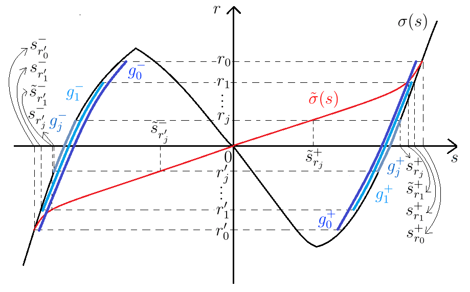
Figure 9. Modified flux $\tilde{\sigma}(s)$ and iteration scheme

For each $j\geq 1$, let $\tilde{s}^{+}_{r_{j}}\in(0,s^{+}_{r_{j}})$ and $\tilde{s}^{-}_{r_{j}^{\prime}}\in(s^{-}_{r_{j}^{\prime}},0)$ denote the unique numbers with $\tilde{\sigma}(\tilde{s}^{+}_{r_{j}})=r_{j}$ and $\tilde{\sigma}(\tilde{s}^{-}_{r_{j}^{\prime}})=r_{j}^{\prime}$, respectively. By Theorem 3.1, for each $j\geq 1$, we can inductively choose a time $t_{j}\in(t_{j-1},\infty)$ with $t_{j}>j$ such that

(7.3) $$\tilde{s}^{-}_{r_{j}^{\prime}}<\min_{\bar{\Omega}}u^{*}_{x}(\cdot,t_{j})\leq 0\leq\max_{\bar{\Omega}}u^{*}_{x}(\cdot,t_{j})<\tilde{s}^{+}_{r_{j}},$$

where $t_{0}:=0$.

Define

$$Q_{0}=\big{\{}(x,t)\in\Omega\times(t_{0},t_{1})\,|\,s^{-}_{r_{0}^{\prime}}<u^{*}_{x}(x,t)<s^{+}_{r_{0}}\big{\}}.$$

Also, for each $j\geq 1$, define

$$Q_{j}=\big{\{}(x,t)\in\Omega\times(t_{j},t_{j+1})\,|\,\tilde{s}^{-}_{r_{j}^{\prime}}<u^{*}_{x}(x,t)<\tilde{s}^{+}_{r_{j}}\big{\}};$$

then from Theorem 3.1 and (7.3), we have $Q_{j}=\Omega\times(t_{j},t_{j+1})$. For each $j\geq 1$, we also let $u_{j}=u^{*}(\cdot,t_{j})\in C^{2+\alpha}(\bar{\Omega})$ so that $u_{j}^{\prime}=0$ on $\partial\Omega$.

Next, for each $j\geq 0$, let

$$g_{j}^{\pm}=g_{r_{j}^{\prime},r_{j};\pm}=(\sigma|_{[s^{\pm}_{r_{j}^{\prime}},s^{\pm}_{r_{j}}]})^{-1}:[r_{j}^{\prime},r_{j}]\to[s^{\pm}_{r_{j}^{\prime}},s^{\pm}_{r_{j}}];$$

then $g^{-}_{j}\leq g^{-}_{j}(r_{j})=s^{-}_{r_{j}}<0<s^{+}_{r_{j}^{\prime}}=g^{+}_{j}(r_{j}^{\prime})\leq g^{+}_{j}$ on $[r_{j}^{\prime},r_{j}]$ (see Figure 9).

Fix an integer $j\geq 0$ here and below. Let $b_{j}=\|u^{*}_{t}\|_{L^{\infty}(Q_{j})}+1$. With the functions $g^{\pm}_{j}$ above, for each $u\in\mathbb{R}$, let $K_{b_{j}}(u)=K_{g^{+}_{j},g^{-}_{j};b_{j}}(u)$ and $U_{b_{j}}(u)=U_{g^{+}_{j},g^{-}_{j};b_{j}}(u)$ be defined as in Subsection 3.5. From (7.1), (7.2) and the definition of $b_{j}$, it follows that

$$\nabla w^{*}\in U_{b_{j}}(u^{*})\;\;\mbox{in $Q_{j}$};$$

thus $w^{*}|_{Q_{j}}$ becomes a strict subsolution of differential inclusion (3.3) with $Q=Q_{j}$ so that $0<\Gamma^{Q_{j}}_{w^{*}}<1$, where the gauge operator $\Gamma^{Q_{j}}_{\cdot}=\Gamma^{Q_{j}}_{g^{+}_{j},g^{-}_{j};\cdot}$ is given as in Subsection 3.5.

Admissible class in the $j^{th}$ step

With $\epsilon=\min\{2^{-j},j^{-1}\Gamma^{Q_{j}}_{w^{*}}\}$ and the above notation, let $\mathcal{A}_{j}=\mathcal{A}_{g_{j}^{+},g_{j}^{-},b_{j},w^{*},Q_{j},\epsilon}$ and $\mathcal{A}_{j,\delta}=\mathcal{A}_{g_{j}^{+},g_{j}^{-},b_{j},w^{*},Q_{j},\epsilon;\delta}$ $(\delta>0)$ be defined as in Subsection 3.5. We then define a class $\mathfrak{A}_{j}$ of admissible functions by the following: for $j=0$, we take

$$\mathfrak{A}_{0}=\left\{\begin{array}[]{l}w^{(0)}=(u^{(0)},v^{(0)})\in\\ (C^{2,1}\times C^{3,1})(\bar{\Omega}\times[t_{0},t_{1}])\end{array}\,\Big{|}\,\begin{array}[]{l}\mbox{$w^{(0)}=w^{*}$ in}\\ \mbox{$(\Omega\times(t_{0},t_{1}))\setminus Q_{0}$,}\\ \mbox{$w^{(j)}|_{Q_{0}}\in\mathcal{A}_{0}$}\end{array}\right\},$$

and for $j\geq 1$, we simply let $\mathfrak{A}_{j}=\mathcal{A}_{j}$; then $w^{*}|_{\Omega\times(t_{0},t_{1})}\in\mathfrak{A}_{0}$ and $w^{*}|_{Q_{j}}\in\mathfrak{A}_{j}$ $\forall j\geq 1$. Also, for each $\delta>0,$ let $\mathfrak{A}_{j,\delta}$ be the subclass of functions $w^{(j)}\in\mathfrak{A}_{j}$ with $w^{(j)}|_{Q_{j}}\in\mathcal{A}_{j,\delta}$.

Baire’s category method in the $j^{th}$ step

Let $\mathfrak{X}_{j}$ denote the closure of $\mathfrak{A}_{j}$ in the space $L^{\infty}(\Omega\times(t_{j},t_{j+1});\mathbb{R}^{2})$; then $(\mathfrak{X}_{j},L^{\infty})$ becomes a nonempty complete metric space. From the definition of $\mathfrak{A}_{j}$, it is easy to check that

$$\mathfrak{X}_{j}\subset w^{*}+W^{1,\infty}_{0}(\Omega\times(t_{j},t_{j+1});\mathbb{R}^{2}).$$

As in the proof of Theorem 2.2, we also see that the set of points of continuity for the space-time gradient operator $\nabla_{j}=\nabla:\mathfrak{X}_{j}\to L^{1}(\Omega\times(t_{j},t_{j+1});\mathbb{M}^{2\times 2})$, say $\mathfrak{C}_{\nabla_{j}}$, is dense in $\mathfrak{X}_{j}$.

Solutions over $[t_{j},t_{j+1}]$ from $\mathfrak{C}_{\nabla_{j}}$

Let $w^{(j)}=(u^{(j)},v^{(j)})\in\mathfrak{C}_{\nabla_{j}}$. Repeating the same procedure as in the proof of Theorem 2.6 for Case 1 under the Baire category framework above, we obtain the following:

$$(j=0)\left\{\begin{array}[]{l}\mbox{$w^{(0)}=w^{*}$ in $(\bar{\Omega}\times[t_{0},t_{1}])\setminus Q_{0}$},\\ \mbox{$\nabla w^{(0)}=\nabla w^{*}$ a.e. in $(\Omega\times(t_{0},t_{1}))\setminus Q_{0}$},\\ \mbox{$v^{(0)}_{t}=\sigma(u^{(0)}_{x})$ a.e. in $(\Omega\times(t_{0},t_{1}))\setminus Q_{0}$},\end{array}\right.$$

(7.4) $$\left\{\begin{array}[]{l}\|u^{(j)}-u^{*}\|_{L^{\infty}(Q_{j})}\leq 2^{-(j+1)},\\ \|u^{(j)}_{t}-u^{*}_{t}\|_{L^{\infty}(Q_{j})}\leq 2^{-(j+1)},\\ |\Gamma^{Q_{j}}_{w^{(j)}}-\Gamma^{Q_{j}}_{w^{*}}|\leq\frac{\Gamma^{Q_{j}}_{w^{*}}}{2j},\\ \mbox{$v^{(j)}_{t}=\sigma(u^{(j)}_{x})$ a.e. in $Q_{j}$,}\\ \mbox{$u^{(j)}_{x}\in[s^{-}_{r_{j}^{\prime}},s^{-}_{r_{j}}]\cup[s^{+}_{r_{j}^{\prime}},s^{+}_{r_{j}}]$ a.e. in $Q_{j}$}.\end{array}\right.$$

From the last of this, we see

(7.5) $$\begin{split}\big{\|}\mathrm{dist}\big{(}u^{(j)}_{x}&,\{s^{+}_{0},s^{-}_{0}\}\big{)}\big{\|}_{L^{\infty}(\Omega\times(t_{j},t_{j+1}))}\\ &\leq\max\big{\{}|s^{+}_{r_{j}}-s^{+}_{0}|,|s^{+}_{r_{j}^{\prime}}-s^{+}_{0}|,|s^{-}_{r_{j}}-s^{-}_{0}|,|s^{-}_{r_{j}^{\prime}}-s^{-}_{0}|\big{\}}\;\;(j\geq 1).\end{split}$$

As in the proof of Theorem 2.6 for Case 1, we can also deduce that for any $\zeta\in C^{\infty}(\bar{\Omega}\times[t_{j},t_{j+1}])$ and any $\tau\in[t_{j},t_{j+1}]$,

(7.6) $$\begin{split}\int_{t_{j}}^{\tau}&\int_{0}^{L}u^{(j)}\zeta_{t}\,dxdt\\ &=\int_{t_{j}}^{\tau}\int_{0}^{L}\sigma(u^{(j)}_{x})\zeta_{x}\,dxdt+\int_{0}^{L}\big{(}u^{(j)}(x,\tau)\zeta(x,\tau)-u_{j}(x)\zeta(x,t_{j})\big{)}\,dx.\end{split}$$

Gauge estimate for $w^{*}$ over $[t_{j},t_{j+1}]$

Observe from (7.1), (7.3) and the definition of $Q_{j}$ that at any point $(x,t)\in Q_{j},$

$$\frac{\tilde{d}_{0,j}}{d_{1,j}}\leq Z_{w^{*}}=\frac{u^{*}_{x}-g^{-}_{j}(v^{*}_{t})}{g^{+}_{j}(v^{*}_{t})-g^{-}_{j}(v^{*}_{t})}\leq\frac{\tilde{d}_{1,j}}{d_{0,j}},$$

where $j\geq 1$, $Z_{w^{*}}=Z^{Q_{j}}_{g^{+}_{j},g^{-}_{j};w^{*}}$ is as in Subsection 3.5, and

$$\left\{\begin{array}[]{l}d_{0,j}:=\underset{[r_{j}^{\prime},r_{j}]}{\min}(g^{+}_{j}-g^{-}_{j}),\;\;d_{1,j}:=\underset{[r_{j}^{\prime},r_{j}]}{\max}(g^{+}_{j}-g^{-}_{j}),\\ \tilde{d}_{0,j}:=\underset{[r_{j}^{\prime},r_{j}]}{\min}(\tilde{g}_{j}-g^{-}_{j}),\;\;\tilde{d}_{1,j}:=\underset{[r_{j}^{\prime},r_{j}]}{\max}(\tilde{g}_{j}-g^{-}_{j}),\end{array}\right.$$

with $\tilde{g}_{j}:=(\tilde{\sigma}|_{[\tilde{s}^{-}_{r_{j}^{\prime}},\tilde{s}^{+}_{r_{j}}]})^{-1}:[r_{j}^{\prime},r_{j}]\to[\tilde{s}^{-}_{r_{j}^{\prime}},\tilde{s}^{+}_{r_{j}}]$. We thus have

(7.7) $$\frac{\tilde{d}_{0,j}}{d_{1,j}}\leq\Gamma^{Q_{j}}_{w^{*}}\leq\frac{\tilde{d}_{1,j}}{d_{0,j}}\;\;(j\geq 1).$$

On the other hand, it is easy to check that

$$\lim_{j\to\infty}\frac{\tilde{d}_{0,j}}{d_{1,j}}=\lim_{j\to\infty}\frac{\tilde{d}_{1,j}}{d_{0,j}}=\frac{-s^{-}_{0}}{s^{+}_{0}-s^{-}_{0}}=\lambda_{0}\in(0,1).$$

To see this, choose two numbers $r_{1,j},\tilde{r}_{0,j}\in[r_{j}^{\prime},r_{j}]$ such that

$$g^{+}_{j}(r_{1,j})-g^{-}_{j}(r_{1,j})=d_{1,j}\;\;\mbox{and}\;\;\tilde{g}_{j}(\tilde{r}_{0,j})-g^{-}_{j}(\tilde{r}_{0,j})=\tilde{d}_{0,j}.$$

As $j\to\infty$, we have $r_{1,j},\tilde{r}_{0,j}\to 0$, and so

$$d_{1,j}=g^{+}_{j}(r_{1,j})-g^{-}_{j}(r_{1,j})\longrightarrow s^{+}_{0}-s^{-}_{0},$$

$$\tilde{d}_{0,j}=\tilde{g}_{j}(\tilde{r}_{0,j})-g^{-}_{j}(\tilde{r}_{0,j})\longrightarrow-s^{-}_{0}.$$

Thus $\underset{j\to\infty}{\lim}\frac{\tilde{d}_{0,j}}{d_{1,j}}=\lambda_{0}$, and the other limit can be shown in the same way.

Energy estimate in the $j^{th}$ step

We now consider the quantity

$$\begin{split}\frac{1}{t_{j+1}-t_{j}}\int_{t_{j}}^{t_{j+1}}\mathcal{E}(u^{(j)}(\cdot,t))&\,dt=\frac{1}{t_{j+1}-t_{j}}\int_{t_{j}}^{t_{j+1}}\int_{\Omega}W(u^{(j)}_{x}(x,t))\,dxdt\\ &=\frac{1}{t_{j+1}-t_{j}}\bigg{(}\int_{Q^{+}_{j}}+\int_{Q^{-}_{j}}\bigg{)}W(u^{(j)}_{x})=:I^{+}_{j}+I^{-}_{j},\end{split}$$

where $j\geq 1$, and $Q_{j}=\Omega\times(t_{j},t_{j+1})$ is divided into the two sets $Q^{\pm}_{j}$ up to measure zero by the last of (7.4):

$$\begin{split}Q^{\pm}_{j}=\big{\{}(x,t)\in Q_{j}\,|\,u^{(j)}_{x}(x,t)\in[s^{\pm}_{r_{j}^{\prime}},s^{\pm}_{r_{j}}]\big{\}}.\end{split}$$

From the third of (7.4), (7.7) and the definition of $\Gamma^{Q_{j}}_{\cdot}$, we have

$$\begin{split}\Big{(}1-\frac{1}{2j}\Big{)}\frac{\tilde{d}_{0,j}}{d_{1,j}}&\leq\Big{(}1-\frac{1}{2j}\Big{)}\Gamma^{Q_{j}}_{w^{*}}\leq\frac{|Q^{+}_{j}|}{|Q_{j}|}=\Gamma^{Q_{j}}_{w^{(j)}}\\ &\leq\Big{(}1+\frac{1}{2j}\Big{)}\Gamma^{Q_{j}}_{w^{*}}\leq\Big{(}1+\frac{1}{2j}\Big{)}\frac{\tilde{d}_{1,j}}{d_{0,j}};\end{split}$$

hence

$$\Big{(}1-\frac{1}{2j}\Big{)}\frac{\tilde{d}_{0,j}}{d_{1,j}}|Q_{j}|\leq|Q^{+}_{j}|\leq\Big{(}1+\frac{1}{2j}\Big{)}\frac{\tilde{d}_{1,j}}{d_{0,j}}|Q_{j}|.$$

Using this, we get

$$\begin{split}L\Big{(}1-\frac{1}{2j}\Big{)}\frac{\tilde{d}_{0,j}}{d_{1,j}}W(s^{+}_{0})&\leq\frac{1}{t_{j+1}-t_{j}}W(s^{+}_{0})|Q^{+}_{j}|\leq I^{+}_{j}\\ &\leq\frac{1}{t_{j+1}-t_{j}}\max\big{\{}W(s^{+}_{r_{j}}),W(s^{+}_{r_{j}^{\prime}})\big{\}}|Q^{+}_{j}|\\ &\leq L\Big{(}1+\frac{1}{2j}\Big{)}\frac{\tilde{d}_{1,j}}{d_{0,j}}\max\big{\{}W(s^{+}_{r_{j}}),W(s^{+}_{r_{j}^{\prime}})\big{\}}.\end{split}$$

Note here that the far left and right terms are approaching $L\lambda_{0}W(s^{+}_{0})$ as $j\to\infty$; that is, $\underset{j\to\infty}{\lim}I^{+}_{j}=L\lambda_{0}W(s^{+}_{0})$. In a similar way, one can check that $\underset{j\to\infty}{\lim}I^{-}_{j}=L(1-\lambda_{0})W(s^{-}_{0})$; we omit the details. Therefore, as $j\to\infty$,

(7.8) $$\frac{1}{t_{j+1}-t_{j}}\int_{t_{j}}^{t_{j+1}}\mathcal{E}(u^{(j)}(\cdot,t))\,dt\longrightarrow L\big{(}\lambda_{0}W(s^{+}_{0})+(1-\lambda_{0})W(s^{-}_{0})\big{)}.$$

Solutions by patching

At this final stage, we check that the set

$$\mathcal{S}:=\Bigg{\{}u=\sum_{j=0}^{\infty}u^{(j)}\chi_{\bar{\Omega}\times[t_{j},t_{j+1})}\,\Big{|}\,w^{(j)}=(u^{(j)},v^{(j)})\in\mathfrak{C}_{\nabla_{j}}\;\;\forall j\geq 0\Bigg{\}}$$

consists of infinitely many global weak solutions $u$ to problem (1.1) satisfying (1)–(3).

As in the proof of Theorem 2.6 for Case 1, we easily see that $\mathcal{S}$ is an infinite set.

Let $u\in\mathcal{S}$. Then (1) follows from the first of (7.4) and (4) of Theorem 3.1. Moreover, (2) and (3) are an immediate consequence of (7.5) and (7.8), respectively.

The proof of Theorem 2.7 is finally complete.

8. Proof of density lemma

In this final section, we provide a long proof of the density lemma, Lemma 3.5.

To start the proof, fix any $\delta>0$, and let $w=(u,v)\in\mathcal{A}$; that is,

(8.1) $$\left\{\begin{array}[]{l}\mbox{$w\in(C^{2,1}\times C^{3,1})(\bar{Q})$, $w$ is Lipschitz in $Q$,}\\ \mbox{$w=w^{*}$ in $Q\setminus\bar{Q}^{w}$ for some open set $Q^{w}\subset\subset Q$ with $|\partial Q^{w}|=0$,}\\ \mbox{$\|u-u^{*}\|_{L^{\infty}(Q)}<\epsilon/2$, $\|u_{t}-u_{t}^{*}\|_{L^{\infty}(Q)}<\epsilon/2$, $|\Gamma^{Q}_{w}-\Gamma^{Q}_{w^{*}}|<\epsilon/2$, }\\ \mbox{$\nabla w\in U_{b}(u)$ in $Q$}.\end{array}\right.$$

Let $\eta>0$. Our goal is to construct a function $w_{\eta}=(u_{\eta},v_{\eta})\in\mathcal{A}_{\delta}$ with $\|w_{\eta}-w\|_{L^{\infty}(Q)}<\eta$, that is, a function $w_{\eta}\in(C^{2,1}\times C^{3,1})(\bar{Q})$ such that

(8.2) $$\left\{\begin{array}[]{l}\mbox{$w_{\eta}$ is Lipschitz in $Q$, $\|w_{\eta}-w\|_{L^{\infty}(Q)}<\eta$,}\\ \mbox{$w_{\eta}=w^{*}$ in $Q\setminus\bar{Q}^{w_{\eta}}$ for some open set $Q^{w_{\eta}}\subset\subset Q$ with $|\partial Q^{w_{\eta}}|=0$,}\\ \mbox{$\|u_{\eta}-u^{*}\|_{L^{\infty}(Q)}<\epsilon/2$, $\|(u_{\eta})_{t}-u_{t}^{*}\|_{L^{\infty}(Q)}<\epsilon/2$, $|\Gamma^{Q}_{w_{\eta}}-\Gamma^{Q}_{w^{*}}|<\epsilon/2$, }\\ \mbox{$\nabla w_{\eta}\in U_{b}(u_{\eta})$ in $Q$, $\int_{Q}\mathrm{dist}\big{(}\nabla w_{\eta}(x,t),K_{b}(u_{\eta}(x,t))\big{)}\,dxdt\leq\delta|Q|$}.\end{array}\right.$$

As the construction is long and complicated, we divide it into many steps.

Step 1

We first choose an open set $G\subset\subset Q\setminus\partial Q^{w}$ with $|\partial G|=0$ such that

(8.3) $$\int_{Q\setminus\bar{G}}\mathrm{dist}\big{(}\nabla w(x,t),K_{b}(u(x,t))\big{)}\,dxdt\leq\frac{\delta}{k}|Q|,$$

where $k\in\mathbb{N}$ is to be specified later.

By (8.1), we have

$$(u_{x},v_{t})\in\tilde{U}\;\;\mbox{and}\;\;|u_{t}|<b\;\;\mbox{on $\bar{G}$};$$

so

(8.4) $$d^{\prime}:=\min_{\bar{G}}\mathrm{dist}\big{(}(u_{x},v_{t}),\partial\tilde{U}\big{)}>0\;\;\mbox{and}\;\;b^{\prime}:=b-\max_{\bar{G}}|u_{t}|>0.$$

Also, by (8.1), we have

$$d^{\prime\prime}:=(\epsilon/2-|\Gamma^{Q}_{w}-\Gamma^{Q}_{w^{*}}|)/2>0.$$

By the uniform continuity of $g^{\pm}$ on $[r_{1},r_{2}]$, we can choose a $\kappa>0$ such that

(8.5) $$|g^{\pm}(r)-g^{\pm}(r^{\prime})|\leq d^{\prime\prime}/l r,r^{\prime}\in[r_{1},r_{2}] |r-r^{\prime}|\leq\kappa,$$ whenever and

where $l\in\mathbb{N}$ will be chosen later.

Now, we choose finitely many disjoint open squares $Q_{1},\cdots,Q_{N}\subset G$, parallel to the axes, such that

(8.6) $$\int_{G\setminus(\cup_{i=1}^{N}\bar{Q}_{i})}\mathrm{dist}\big{(}\nabla w(x,t),K_{b}(u(x,t))\big{)}\,dxdt\leq\frac{\delta}{k}|Q|.$$

Dividing these squares $Q_{1},\cdots,Q_{N}$ into disjoint open sub-squares up to measure zero if necessary, we can have that

(8.7) $$\big{|}\big{(}u_{x}(x_{1},t_{1}),v_{t}(x_{1},t_{1})\big{)}-\big{(}u_{x}(x_{2},t_{2}),v_{t}(x_{2},t_{2})\big{)}\big{|}\leq\min\Big{\{}\frac{\delta}{4k},\frac{d^{\prime}}{4},\frac{\kappa}{2}\Big{\}}$$

and

(8.8) $$|u_{t}(x_{1},t_{1})-u_{t}(x_{2},t_{2})|\leq\frac{b^{\prime}}{4}$$

whenever $(x_{1},t_{1}),(x_{2},t_{2})\in\bar{Q}_{i}$ and $1\leq i\leq N$.

Step 2

Consider the two continuous functions $f^{\pm}:[0,\infty)\to[0,\infty)$ defined by

$$f^{\pm}(\beta)=\min_{r,r^{\prime}\in[r_{1},r_{2}]}\big{|}\big{(}g^{\pm}(r)\mp\beta,r\big{)}-\big{(}g^{\pm}(r^{\prime}),r^{\prime}\big{)}\big{|}\;\;\forall\beta\geq 0;$$

then $f^{\pm}$ are strictly increasing on $[0,\infty)$ with $f^{\pm}(0)=0$ and $\underset{\beta\to\infty}{\lim}f^{\pm}(\beta)=\infty$. So we can choose two unique numbers $\beta^{\pm}_{k}>0$ such that $f^{\pm}(\beta^{\pm}_{k})=\frac{\delta}{k-1},$ where we let $k\in\mathbb{N}$ satisfy

(8.9) $$k\geq 2.$$

We also choose $k\in\mathbb{N}$ so large that

(8.10) $$g^{-}(r)+\beta^{-}_{k}<g^{+}(r)-\beta^{+}_{k}\;\;\forall r\in[r_{1},r_{2}].$$

We then define two disjoint bounded domains $D^{\pm}_{k}\subset\tilde{U}$ by

$$\begin{split}D^{+}_{k}&=\big{\{}(s,r)\in\mathbb{R}^{2}\,|\,r_{1}<r<r_{2},g^{+}(r)-\beta^{+}_{k}<s<g^{+}(r)\big{\}},\\ D^{-}_{k}&=\big{\{}(s,r)\in\mathbb{R}^{2}\,|\,r_{1}<r<r_{2},g^{-}(r)<s<g^{-}(r)+\beta^{-}_{k}\big{\}}.\end{split}$$

Fix an index $i\in\mathcal{I}:=\{1,\cdots,N\}$, and let us denote by $(x_{i},t_{i})$ the center of the square $Q_{i}$. We also write

$$(s_{i},\gamma_{i})=\big{(}u_{x}(x_{i},t_{i}),v_{t}(x_{i},t_{i})\big{)}\;\;\mbox{and}\;\;c_{i}=u_{t}(x_{i},t_{i});$$

then $(s_{i},\gamma_{i})\in\tilde{U}$ and $|c_{i}|\leq b-b^{\prime}.$

Next, we split the index set $\mathcal{I}$ into the three sets

$$\mathcal{I}^{\pm}_{1}:=\big{\{}i\in\mathcal{I}\,|\,\mathrm{dist}\big{(}(s_{i},\gamma_{i}),\tilde{K}^{\pm}\big{)}\leq\delta/k\big{\}}\;\;\mbox{and}\;\;\mathcal{I}_{2}:=\mathcal{I}\setminus(\mathcal{I}^{+}_{1}\cup\mathcal{I}^{-}_{1}).$$

It is then easy to check that $(s_{i},\gamma_{i})\in D^{\pm}_{k}$ for all $i\in\mathcal{I}^{\pm}_{1}$; thus $\mathcal{I}^{+}_{1}\cap\mathcal{I}^{-}_{1}=\emptyset$.

Let $i\in\mathcal{I}^{+}_{1}$. Then there exists a $\bar{\gamma_{i}}\in[r_{1},r_{2}]$ such that

(8.11) $$\big{|}(s_{i},\gamma_{i})-\big{(}g^{+}(\bar{\gamma_{i}}),\bar{\gamma_{i}}\big{)}\big{|}\leq\frac{\delta}{k}.$$

Let $(x,t)\in Q_{i}$; then by (8.1), (8.7) and (8.11), we have

$$\left|\begin{pmatrix}u_{x}(x,t)&u_{t}(x,t)\\ v_{x}(x,t)&v_{t}(x,t)\end{pmatrix}-\begin{pmatrix}g^{+}(\bar{\gamma_{i}})&u_{t}(x,t)\\ u(x,t)&\bar{\gamma_{i}}\end{pmatrix}\right|\leq\frac{5\delta}{4k},$$

where

$$\begin{pmatrix}g^{+}(\bar{\gamma_{i}})&u_{t}(x,t)\\ u(x,t)&\bar{\gamma_{i}}\end{pmatrix}\in K_{b}(u(x,t)).$$

So

$$\int_{Q_{i}}\mathrm{dist}\big{(}\nabla w(x,t),K_{b}(u(x,t))\big{)}\,dxdt\leq\frac{5\delta}{4k}|Q_{i}|,$$

and the same inequality can be shown to hold in a similar manner when $i\in\mathcal{I}^{-}_{1}.$ We thus have

(8.12) $$\int_{\cup_{i\in\mathcal{I}^{+}_{1}\cup\mathcal{I}^{-}_{1}}Q_{i}}\mathrm{dist}\big{(}\nabla w(x,t),K_{b}(u(x,t))\big{)}\,dxdt\leq\frac{5\delta}{4k}|Q|.$$

Step 3

Fix an index $i\in\mathcal{I}_{2}$. Since $\mathrm{dist}\big{(}(s_{i},\gamma_{i}),\tilde{K}^{\pm}\big{)}>\delta/k$, we can choose two positive numbers $\lambda_{i}^{\pm}$ so that

(8.13) $$\left\{\begin{array}[]{l}\mathrm{dist}\big{(}(s_{i}+\lambda_{i}^{+},\gamma_{i}),\tilde{K}^{+}\big{)}=\delta/k,\;(s_{i}+\lambda_{i}^{+},\gamma_{i})\in D^{+}_{k},\\ \mathrm{dist}\big{(}(s_{i}-\lambda_{i}^{-},\gamma_{i}),\tilde{K}^{-}\big{)}=\delta/k,\;(s_{i}-\lambda_{i}^{-},\gamma_{i})\in D^{-}_{k}.\end{array}\right.$$

For a given $\epsilon_{i}>0$ to be specified later, we can apply Lemma 3.4 to obtain a function $\omega_{i}=(\varphi_{i},\psi_{i})\in C^{\infty}_{c}(Q_{i};\mathbb{R}^{2})$ such that

• $\|\omega_{i}\|_{L^{\infty}(Q_{i})}<\epsilon_{i}$, $\|(\varphi_{i})_{t}\|_{L^{\infty}(Q_{i})}<\epsilon_{i}$, $\|(\psi_{i})_{t}\|_{L^{\infty}(Q_{i})}<\epsilon_{i}$,

• $-\lambda_{i}^{-}\leq(\varphi_{i})_{x}\leq\lambda_{i}^{+}$ in $Q_{i}$,

• $\left\{\begin{array}[]{l}\big{|}|\{(x,t)\in Q_{i}\,|\,(\varphi_{i})_{x}(x,t)=\lambda_{i}^{+}\}|-\frac{\lambda_{i}^{-}}{\lambda_{i}^{+}+\lambda_{i}^{-}}|Q_{i}|\big{|}<\epsilon_{i},\\ \big{|}|\{(x,t)\in Q_{i}\,|\,(\varphi_{i})_{x}(x,t)=-\lambda_{i}^{-}\}|-\frac{\lambda_{i}^{+}}{\lambda_{i}^{+}+\lambda_{i}^{-}}|Q_{i}|\big{|}<\epsilon_{i},\end{array}\right.$

• $(\psi_{i})_{x}=\varphi_{i}$ in $Q_{i}$, and

• $\int_{x_{i,1}}^{x_{i,2}}\varphi_{i}(x,t)\,dx=0$ for all $t_{i,1}<t<t_{i,2}$,

where $Q_{i}=(x_{i,1},x_{i,2})\times(t_{i,1},t_{i,2})$. We now define

(8.14) $$w_{\eta}=(u_{\eta},v_{\eta})=w+\sum_{i\in\mathcal{I}_{2}}\omega_{i}\chi_{Q_{i}}\;\;\mbox{in $Q$}.$$

Step 4

To finish the proof, we show that upon choosing suitable numbers $l,k\in\mathbb{N}$ and $\epsilon_{i}>0$ $(i\in\mathcal{I}_{2})$, the function $w_{\eta}=(u_{\eta},v_{\eta})$ defined in (8.14) satisfies the desired properties in (8.2). Since this step consists of many arguments to verify, we separate it into several substeps.

Substep 4-1

We begin with simpler parts to prove.

From (8.1) and (8.14), it follows that

(8.15) $$w_{\eta}\in(C^{2,1}\times C^{3,1})(\bar{Q}) Q$$ is Lipschitz in .

Set $Q^{w_{\eta}}=G\cup Q^{w}$; then $Q^{w_{\eta}}\subset\subset Q$ is an open set with $|\partial Q^{w_{\eta}}|=0$. From (8.1) and (8.14), we also have

(8.16) $$w_{\eta}=w=w^{*}\;\;\mbox{in $Q\setminus\bar{Q}^{w_{\eta}}$}.$$

Next, we choose

(8.17) $$\epsilon_{i}<\min\Big{\{}\eta,\;\frac{\epsilon}{2}-\|u-u^{*}\|_{L^{\infty}(Q)},\,\frac{\epsilon}{2}-\|u_{t}-u^{*}_{t}\|_{L^{\infty}(Q)}\Big{\}} i\in\mathcal{I}_{2}$$  for all ;

then from (a) and (8.14), we have

(8.18) $$\begin{cases}\|w_{\eta}-w\|_{L^{\infty}(Q)}<\eta,\\ \|u_{\eta}-u^{*}\|_{L^{\infty}(Q)}<{\epsilon}/{2},\\ \|(u_{\eta})_{t}-u^{*}_{t}\|_{L^{\infty}(Q)}<{\epsilon}/{2}.\end{cases}$$

Substep 4-2

In this substep, we show that

(8.19) $$\nabla{w}_{\eta}(x,t)\in U_{b}(u_{\eta}(x,t))\;\;\forall(x,t)\in Q.$$

Note from (8.8), (8.14) and (a) that

$$\begin{split}|(u_{\eta})_{t}(x,t)|&=|u_{t}(x,t)+(\varphi_{i})_{t}(x,t)|\leq|u_{t}(x,t)-c_{i}|+|c_{i}|+|(\varphi_{i})_{t}(x,t)|\\ &\leq\frac{b^{\prime}}{4}+b-b^{\prime}+\epsilon_{i}<b-\frac{b^{\prime}}{2}\;\;\forall(x,t)\in Q_{i},\,\forall i\in\mathcal{I}_{2},\end{split}$$

where we let

(8.20) $$\epsilon_{i}<b^{\prime}/4 \forall i\in\mathcal{I}_{2}$$  .

This implies that

(8.21) $$|(u_{\eta})_{t}(x,t)|<b\;\;\forall(x,t)\in Q.$$

From (8.1), we have $v_{x}=u$ in $Q$. Thus by (8.14) and (d), we have

$$\begin{split}(v_{\eta})_{x}(x,t)&=v_{x}(x,t)+(\psi_{i})_{x}(x,t)\\ &=u(x,t)+\varphi_{i}(x,t)=u_{\eta}(x,t)\;\;\forall(x,t)\in Q_{i},\end{split}$$

where $i\in\mathcal{I}_{2}$; thus

(8.22) $$(v_{\eta})_{x}(x,t)=u_{\eta}(x,t)\;\;\forall(x,t)\in Q.$$

Let $i\in\mathcal{I}_{2}$. From (8.4) and (8.13), we see that

(8.23) $$\mathrm{dist}\big{(}[(s_{i}-\lambda_{i}^{-},\gamma_{i}),(s_{i}+\lambda_{i}^{+},\gamma_{i})],\partial\tilde{U}\big{)}\geq\min\Big{\{}\frac{\delta}{k},d^{\prime}\Big{\}}.$$

Let $(x,t)\in Q_{i}.$ Then by (a) and (8.7),

$$\begin{split}\big{|}\big{(}(u_{\eta})_{x}(x,t),&(v_{\eta})_{t}(x,t)\big{)}-\big{(}s_{i}+(\varphi_{i})_{x}(x,t),\gamma_{i}\big{)}\big{|}\\ \leq&\big{|}\big{(}u_{x}(x,t),v_{t}(x,t)\big{)}-(s_{i},\gamma_{i})\big{|}+|(\psi_{i})_{t}(x,t)|\\ \leq&\min\Big{\{}\frac{\delta}{4k},\frac{d^{\prime}}{4}\Big{\}}+\epsilon_{i}<\min\Big{\{}\frac{\delta}{2k},\frac{d^{\prime}}{2}\Big{\}},\end{split}$$

where we let

(8.24) $$\epsilon_{i}<\min\Big{\{}\frac{\delta}{4k},\frac{d^{\prime}}{4}\Big{\}}.$$

By (b), we have $-\lambda_{i}^{-}\leq(\varphi_{i})_{x}(x,t)\leq\lambda_{i}^{+}$, and so it follows from (8.23) and the previous inequality that

$$\big{(}(u_{\eta})_{x}(x,t),(v_{\eta})_{t}(x,t)\big{)}\in\tilde{U}.$$

Adopting (8.24) for all $i\in\mathcal{I}_{2}$, this inclusion holds for all $(x,t)\in Q.$

This inclusion together with (8.21) and (8.22) implies inclusion (8.19).

Substep 4-3

Here, we prove that

(8.25) $$|\Gamma^{Q}_{w_{\eta}}-\Gamma^{Q}_{w^{*}}|<\frac{\epsilon}{2}.$$

By the definition of the gauge operator $\Gamma^{Q}_{\cdot}$ and (8.14), we have

$$\begin{split}\Gamma^{Q}_{w_{\eta}}-\Gamma^{Q}_{w}=&\frac{1}{|Q|}\int_{Q}\big{(}Z_{w_{\eta}}(x,t)-Z_{w}(x,t)\big{)}\,dxdt\\ =&\frac{1}{|Q|}\sum_{i\in\mathcal{I}_{2}}\int_{Q_{i}}\big{(}Z_{w+\omega_{i}}(x,t)-Z_{w}(x,t)\big{)}\,dxdt\\ =&\frac{1}{|Q|}\sum_{i\in\mathcal{I}_{2}}\bigg{(}\int_{Q_{i,1}}+\int_{Q^{+}_{i,2}}+\int_{Q^{-}_{i,2}}\bigg{)}(Z_{w+\omega_{i}}-Z_{w}),\end{split}$$

where $\omega_{i}$ is defined to be zero outside its compact support, and

$$\begin{split}Q_{i,1}&:=\big{\{}(x,t)\in Q_{i}\,|\,(\varphi_{i})_{x}(x,t)\not\in\{\lambda_{i}^{+},-\lambda_{i}^{-}\}\big{\}},\\ Q^{+}_{i,2}&:=\big{\{}(x,t)\in Q_{i}\,|\,(\varphi_{i})_{x}(x,t)=\lambda_{i}^{+}\big{\}},\\ Q^{-}_{i,2}&:=\big{\{}(x,t)\in Q_{i}\,|\,(\varphi_{i})_{x}(x,t)=-\lambda_{i}^{-}\big{\}}.\end{split}$$

The trivial part to estimate here follows from (c) as

(8.26) $$\bigg{|}\int_{Q_{i,1}}(Z_{w+\omega_{i}}-Z_{w})\bigg{|}\leq 2|Q_{i,1}|<4\epsilon_{i}\;\;(i\in\mathcal{I}_{2}).$$

Next, let $i\in\mathcal{I}_{2}$ and $(x,t)\in Q^{-}_{i,2}$. Then from (8.7), we have at the point $(x,t)$ here and below that

(8.27) $$\begin{split}\big{|}(u+\varphi_{i})_{x}-&g^{-}\big{(}(v+\psi_{i})_{t}\big{)}\big{|}=\big{|}u_{x}-\lambda_{i}^{-}-g^{-}\big{(}v_{t}+(\psi_{i})_{t}\big{)}\big{|}\\ \leq&|u_{x}-s_{i}|+|s_{i}-\lambda_{i}^{-}-g^{-}(\gamma_{i})|+\big{|}g^{-}(\gamma_{i})-g^{-}\big{(}v_{t}+(\psi_{i})_{t}\big{)}\big{|}\\ \leq&\frac{\delta}{4k}+|s_{i}-\lambda_{i}^{-}-g^{-}(\gamma_{i})|+\big{|}g^{-}(\gamma_{i})-g^{-}\big{(}v_{t}+(\psi_{i})_{t}\big{)}\big{|}.\end{split}$$

From (8.13), it follows that $\big{|}(s_{i}-\lambda_{i}^{-},\gamma_{i})-\big{(}g^{-}(\bar{\gamma}_{i}),\bar{\gamma}_{i}\big{)}\big{|}=\delta/k$ for some $\bar{\gamma}_{i}\in[r_{1},r_{2}]$. Thus, we have from (8.5) that

(8.28) $$|s_{i}-\lambda_{i}^{-}-g^{-}(\gamma_{i})|\leq|s_{i}-\lambda_{i}^{-}-g^{-}(\bar{\gamma}_{i})|+|g^{-}(\bar{\gamma}_{i})-g^{-}(\gamma_{i})|\leq\frac{\delta}{k}+\frac{d^{\prime\prime}}{l},$$

where we let $k\in\mathbb{N}$ satisfy

(8.29) $$\frac{\delta}{k}\leq\kappa.$$

Likewise, with (8.29), we also have

(8.30) $$|s_{i}+\lambda_{i}^{+}-g^{+}(\gamma_{i})|\leq\frac{\delta}{k}+\frac{d^{\prime\prime}}{l}.$$

Also, from (8.7) and (a), we have

$$\big{|}\gamma_{i}-\big{(}v_{t}+(\psi_{i})_{t}\big{)}\big{|}\leq|\gamma_{i}-v_{t}|+|(\psi_{i})_{t}|\leq\frac{\kappa}{2}+\epsilon_{i}\leq\kappa,$$

where we let

(8.31) $$\epsilon_{i}\leq\frac{\kappa}{2}.$$

With the help of (8.5), this implies that

(8.32) $$\big{|}g^{-}(\gamma_{i})-g^{-}\big{(}v_{t}+(\psi_{i})_{t}\big{)}\big{|}\leq\frac{d^{\prime\prime}}{l}.$$

Thus (8.27), (8.30) and (8.32) yield that

$$\big{|}(u+\varphi_{i})_{x}-g^{-}\big{(}(v+\psi_{i})_{t}\big{)}\big{|}\leq\frac{5\delta}{4k}+\frac{2d^{\prime\prime}}{l}\leq\frac{3d^{\prime\prime}}{l}$$

if we choose $k\in\mathbb{N}$ so large that

(8.33) $$\frac{5\delta}{4k}\leq\frac{d^{\prime\prime}}{l}.$$

Since $g^{+}\big{(}(v+\psi_{i})_{t}\big{)}-g^{-}\big{(}(v+\psi_{i})_{t}\big{)}\geq\underset{[r_{1},r_{2}]}{\min}(g^{+}-g^{-})=:d_{0}>0$, we thus have

$$Z_{w+\omega_{i}}(x,t)\leq\frac{3d^{\prime\prime}}{ld_{0}}\quad\forall\,(x,t)\in Q_{i,2}^{-};$$

hence

(8.34) $$\bigg{|}\int_{Q^{-}_{i,2}}Z_{w+\omega_{i}}\bigg{|}\leq\frac{3d^{\prime\prime}}{ld_{0}}|Q^{-}_{i,2}|.$$

Let $i\in\mathcal{I}_{2}$ and $Q_{i,2}=Q_{i,2}^{+}\cup Q_{i,2}^{-}$. We now estimate the quantity

$$\bigg{|}\int_{Q_{i,2}^{+}}Z_{w+\omega_{i}}-\int_{Q_{i,2}}Z_{w}\bigg{|}.$$

First, we consider

$$\begin{split}\bigg{|}&\int_{Q_{i,2}^{+}}Z_{w+\omega_{i}}(x,t)\,dxdt-\frac{\lambda_{i}^{-}}{\lambda_{i}^{+}+\lambda_{i}^{-}}|Q_{i}|\bigg{|}\\ &\leq\bigg{|}\int_{Q_{i,2}^{+}}\bigg{(}\frac{u_{x}+(\varphi_{i})_{x}-g^{-}\big{(}v_{t}+(\psi_{i})_{t}\big{)}}{g^{+}\big{(}v_{t}+(\psi_{i})_{t}\big{)}-g^{-}\big{(}v_{t}+(\psi_{i})_{t}\big{)}}\\ &\;\;\;\;\quad\quad\quad\;-\frac{s_{i}+\lambda_{i}^{+}-g^{-}(\gamma_{i})}{g^{+}\big{(}v_{t}+(\psi_{i})_{t}\big{)}-g^{-}\big{(}v_{t}+(\psi_{i})_{t}\big{)}}\bigg{)}\,dxdt\bigg{|}\\ &\;\;\;\;+\bigg{|}\int_{Q_{i,2}^{+}}\bigg{(}\frac{s_{i}+\lambda_{i}^{+}-g^{-}(\gamma_{i})}{g^{+}\big{(}v_{t}+(\psi_{i})_{t}\big{)}-g^{-}\big{(}v_{t}+(\psi_{i})_{t}\big{)}}-\frac{s_{i}+\lambda_{i}^{+}-g^{-}(\gamma_{i})}{g^{+}(\gamma_{i})-g^{-}(\gamma_{i})}\bigg{)}\,dxdt\bigg{|}\\ &\;\;\;\;+\bigg{|}\frac{s_{i}+\lambda_{i}^{+}-g^{-}(\gamma_{i})}{g^{+}(\gamma_{i})-g^{-}(\gamma_{i})}|Q^{+}_{i,2}|-\frac{\lambda_{i}^{-}}{\lambda_{i}^{+}+\lambda_{i}^{-}}|Q_{i}|\bigg{|}=:I_{1}+I_{2}+I_{3}.\end{split}$$

Here, let $\epsilon_{i}>0$ satisfy (8.31); then as in (8.32), we have

(8.35) $$\big{|}g^{\pm}\big{(}v_{t}+(\psi_{i})_{t}\big{)}-g^{\pm}(\gamma_{i})\big{|}\leq\frac{d^{\prime\prime}}{l}\;\;\mbox{in $Q^{+}_{i,2}$}.$$

Using this, (8.7) and the fact that $(\varphi_{i})_{x}=\lambda_{i}^{+}$ in $Q^{+}_{i,2}$, we deduce that

$$I_{1}\leq\frac{1}{d_{0}}\Big{(}\frac{\delta}{4k}+\frac{d^{\prime\prime}}{l}\Big{)}|Q^{+}_{i,2}|\leq\frac{6d^{\prime\prime}}{5ld_{0}}|Q^{+}_{i,2}|,$$

where we let $k\in\mathbb{N}$ fulfill (8.33). Having the common denominator in the integrand, we have from (8.35) that

$$I_{2}\leq\big{(}s_{i}+\lambda_{i}^{+}-g^{-}(\gamma_{i})\big{)}\frac{2d^{\prime\prime}}{ld_{0}^{2}}|Q^{+}_{i,2}|\leq\frac{2d^{\prime\prime}d_{1}}{ld_{0}^{2}}|Q^{+}_{i,2}|,$$

where $d_{1}:=\underset{[r_{1},r_{2}]}{\max}(g^{+}-g^{-})$. Note from (8.30) and (c) that

$$\begin{split}I_{3}&\leq\bigg{|}\frac{s_{i}+\lambda_{i}^{+}-g^{-}(\gamma_{i})}{g^{+}(\gamma_{i})-g^{-}(\gamma_{i})}|Q^{+}_{i,2}|-|Q^{+}_{i,2}|\bigg{|}+\bigg{|}|Q^{+}_{i,2}|-\frac{\lambda_{i}^{-}}{\lambda_{i}^{+}+\lambda_{i}^{-}}|Q_{i}|\bigg{|}\\ &\leq\Big{(}\frac{\delta}{k}+\frac{d^{\prime\prime}}{l}\Big{)}\frac{1}{d_{0}}|Q^{+}_{i,2}|+\epsilon_{i}\leq\frac{9d^{\prime\prime}}{5ld_{0}}|Q^{+}_{i,2}|+\epsilon_{i},\end{split}$$

where we let $k\in\mathbb{N}$ also satisfy (8.29) and (8.33). Combining the estimates on $I_{1},$ $I_{2}$ and $I_{3}$, we obtain

(8.36) $$\bigg{|}\int_{Q_{i,2}^{+}}Z_{w+\omega_{i}}(x,t)\,dxdt-\frac{\lambda_{i}^{-}}{\lambda_{i}^{+}+\lambda_{i}^{-}}|Q_{i}|\bigg{|}\leq\bigg{(}\frac{3}{d_{0}}+\frac{2d_{1}}{d_{0}^{2}}\bigg{)}\frac{d^{\prime\prime}}{l}|Q^{+}_{i,2}|+\epsilon_{i}.$$

Second, we handle

$$\begin{split}\bigg{|}\int_{Q_{i,2}}&Z_{w}(x,t)\,dxdt-\frac{\lambda_{i}^{-}}{\lambda_{i}^{+}+\lambda_{i}^{-}}|Q_{i}|\bigg{|}\\ \leq&\bigg{|}\int_{Q_{i,2}}\bigg{(}\frac{u_{x}-g^{-}(v_{t})}{g^{+}(v_{t})-g^{-}(v_{t})}-\frac{\lambda_{i}^{-}}{g^{+}(v_{t})-g^{-}(v_{t})}\bigg{)}\,dxdt\bigg{|}\\ &+\bigg{|}\int_{Q_{i,2}}\frac{\lambda_{i}^{-}}{g^{+}(v_{t})-g^{-}(v_{t})}\,dxdt-\frac{\lambda_{i}^{-}}{g^{+}(\gamma_{i})-g^{-}(\gamma_{i})}|Q_{i,2}|\bigg{|}\\ &+\bigg{|}\frac{\lambda_{i}^{-}}{g^{+}(\gamma_{i})-g^{-}(\gamma_{i})}|Q_{i,2}|-\frac{\lambda_{i}^{-}}{\lambda_{i}^{+}+\lambda_{i}^{-}}|Q_{i}|\bigg{|}=:J_{1}+J_{2}+J_{3}.\end{split}$$

To estimate $J_{1}$, we first note from (8.5), (8.7) and (8.28) that in $Q_{i,2}$,

$$\begin{split}|u_{x}-g^{-}(v_{t})-\lambda_{i}^{-}|&\leq|u_{x}-s_{i}|+|g^{-}(\gamma_{i})-g^{-}(v_{t})|+|s_{i}-\lambda_{i}^{-}-g^{-}(\gamma_{i})|\\ &\leq\frac{\delta}{4k}+\frac{d^{\prime\prime}}{l}+\Big{(}\frac{\delta}{k}+\frac{d^{\prime\prime}}{l}\Big{)}\leq\ \frac{3d^{\prime\prime}}{l},\end{split}$$

where we let $k\in\mathbb{N}$ satisfy (8.29) and (8.33). From this, we get

$$J_{1}\leq\frac{3d^{\prime\prime}}{ld_{0}}|Q_{i,2}|.$$

From (8.5) and (8.7), we have

$$J_{2}\leq\frac{2\lambda_{i}^{-}d^{\prime\prime}}{ld_{0}^{2}}|Q_{i,2}|\leq\frac{2d^{\prime\prime}d_{1}}{ld_{0}^{2}}|Q_{i,2}|.$$

To estimate $J_{3}$, we observe from (8.28) and (8.30) that

$$\begin{split}\big{|}\lambda_{i}^{+}+\lambda_{i}^{-}-\big{(}g^{+}(\gamma_{i})-g^{-}(\gamma_{i})\big{)}\big{|}&=\big{|}s_{i}+\lambda_{i}^{+}-g^{+}(\gamma_{i})-\big{(}s_{i}-\lambda_{i}^{-}-g^{-}(\gamma_{i})\big{)}\big{|}\\ &\leq\frac{2\delta}{k}+\frac{2d^{\prime\prime}}{l}\leq\frac{18d^{\prime\prime}}{5l},\end{split}$$

with $k\in\mathbb{N}$ satisfying (8.29) and (8.33). Note from this and (c) that

$$\begin{split}J_{3}\leq&\bigg{|}\frac{\lambda_{i}^{-}}{g^{+}(\gamma_{i})-g^{-}(\gamma_{i})}|Q_{i,2}|-\frac{\lambda_{i}^{-}}{\lambda_{i}^{+}+\lambda_{i}^{-}}|Q_{i,2}|\bigg{|}\\ &+\bigg{|}\frac{\lambda_{i}^{-}}{\lambda_{i}^{+}+\lambda_{i}^{-}}|Q_{i,2}|-\frac{\lambda_{i}^{-}}{\lambda_{i}^{+}+\lambda_{i}^{-}}|Q_{i}|\bigg{|}\\ \leq&\frac{18d^{\prime\prime}d_{1}}{5ld_{0}^{2}}|Q_{i,2}|+2\epsilon_{i}.\end{split}$$

By the estimates on $J_{1}$, $J_{2}$ and $J_{3}$, we now have

$$\bigg{|}\int_{Q_{i,2}}Z_{w}(x,t)\,dxdt-\frac{\lambda_{i}^{-}}{\lambda_{i}^{+}+\lambda_{i}^{-}}|Q_{i}|\bigg{|}\leq\bigg{(}\frac{3}{d_{0}}+\frac{28d_{1}}{5d_{0}^{2}}\bigg{)}\frac{d^{\prime\prime}}{l}|Q_{i,2}|+2\epsilon_{i}.$$

Combining this estimate with (8.36), we have

(8.37) $$\begin{split}\bigg{|}\int_{Q_{i,2}^{+}}&Z_{w+\omega_{i}}-\int_{Q_{i,2}}Z_{w}\bigg{|}\\ &\quad\quad\quad\leq\bigg{(}\frac{6}{d_{0}}+\frac{38d_{1}}{5d_{0}^{2}}\bigg{)}\frac{d^{\prime\prime}}{l}|Q_{i,2}|+3\epsilon_{i}.\end{split}$$

Thanks to the estimates (8.26), (8.34) and (8.37), it follows that for all $i\in\mathcal{I}_{2},$

$$\begin{split}\bigg{|}\bigg{(}\int_{Q_{i,1}}+&\int_{Q^{+}_{i,2}}+\int_{Q^{-}_{i,2}}\bigg{)}(Z_{w+\omega_{i}}-Z_{w})\bigg{|}\\ &\leq\bigg{(}\frac{9}{d_{0}}+\frac{38d_{1}}{5d_{0}^{2}}\bigg{)}\frac{d^{\prime\prime}}{l}|Q_{i,2}|+7\epsilon_{i}\leq\frac{17d^{\prime\prime}d_{1}}{ld_{0}^{2}}|Q_{i}|+7\epsilon_{i}.\end{split}$$

Summing this over the indices $i\in\mathcal{I}_{2},$ we then have

$$|\Gamma^{Q}_{w_{\eta}}-\Gamma^{Q}_{w}|\leq\frac{17d^{\prime\prime}d_{1}}{ld_{0}^{2}}+\frac{7}{|Q|}\sum_{i\in\mathcal{I}_{2}}\epsilon_{i}<d^{\prime\prime}$$

if $l\in\mathbb{N}$ is taken so large that

(8.38) $$\frac{17d_{1}}{ld_{0}^{2}}<\frac{1}{2},$$

$k\in\mathbb{N}$ satisfies (8.29) and (8.33), and the numbers $\epsilon_{i}>0$ $(i\in\mathcal{I}_{2})$ fulfill (8.31) and

(8.39) $$\epsilon_{i}<\frac{d^{\prime\prime}}{14N}|Q|.$$

Under such choices of numbers $l,$ $k$ and $\epsilon_{i}$ $(i\in\mathcal{I}_{2})$, we finally have from (8.1) and the definition of $d^{\prime\prime}$ that

$$\begin{split}|\Gamma^{Q}_{w_{\eta}}-\Gamma^{Q}_{w^{*}}|&\leq|\Gamma^{Q}_{w_{\eta}}-\Gamma^{Q}_{w}|+|\Gamma^{Q}_{w}-\Gamma^{Q}_{w^{*}}|\\ &<d^{\prime\prime}+|\Gamma^{Q}_{w}-\Gamma^{Q}_{w^{*}}|=\frac{\epsilon}{4}+\frac{|\Gamma^{Q}_{w}-\Gamma^{Q}_{w^{*}}|}{2}<\frac{\epsilon}{2};\end{split}$$

hence, our goal (8.25) of this substep is indeed achieved.

Substep 4-4

We now prove

(8.40) $$\int_{Q}\mathrm{dist}\big{(}\nabla w_{\eta}(x,t),K_{b}(u_{\eta}(x,t))\big{)}\,dxdt\leq\delta|Q|.$$

Let $i\in\mathcal{I}_{2}$. By (c), we have $|Q_{i,1}|<2\epsilon_{i}$. Let $(x,t)\in Q_{i,1}$ and $r\in[r_{1},r_{2}]$; then by (8.19), we have, at the point $(x,t)$,

$$\begin{split}\bigg{|}\begin{pmatrix}(u_{\eta})_{x}&(u_{\eta})_{t}\\ (v_{\eta})_{x}&(v_{\eta})_{t}\end{pmatrix}&-\begin{pmatrix}g^{+}(r)&(u_{\eta})_{t}\\ u_{\eta}&r\end{pmatrix}\bigg{|}\\ &=\big{|}\big{(}(u_{\eta})_{x},(v_{\eta})_{t}\big{)}-\big{(}g^{+}(r),r\big{)}\big{|}\\ &\leq\mathrm{diam}(\tilde{U}),\end{split}$$

where $\begin{pmatrix}g^{+}(r)&(u_{\eta})_{t}\\ u_{\eta}&r\end{pmatrix}\in K_{b}(u_{\eta})$. Thus, we have

$$\int_{Q_{i,1}}\mathrm{dist}\big{(}\nabla w_{\eta}(x,t),K_{b}(u_{\eta}(x,t))\big{)}\,dxdt\leq 2\epsilon_{i}\mathrm{diam}(\tilde{U})\leq\frac{\delta}{Nk}|Q|,$$

where we let

(8.41) $$\epsilon_{i}\leq\big{(}\mathrm{diam}(\tilde{U})\big{)}^{-1}\frac{\delta}{2Nk}|Q|.$$

Having this choice for all $i\in\mathcal{I}_{2}$, we get

(8.42) $$\sum_{i\in\mathcal{I}_{2}}\int_{Q_{i,1}}\mathrm{dist}\big{(}\nabla w_{\eta}(x,t),K_{b}(u_{\eta}(x,t))\big{)}\,dxdt\leq\frac{\delta}{k}|Q|.$$

Let $i\in\mathcal{I}_{2}$ and $(x,t)\in Q_{i,2}$; then $(\varphi_{i})_{x}(x,t)\in\{\lambda_{i}^{+},-\lambda_{i}^{-}\}$. Suppose $(\varphi_{i})_{x}(x,t)=-\lambda_{i}^{-}.$ By (8.13), we can choose a number $\bar{r}_{i}\in[r_{1},r_{2}]$ such that

$$\big{|}(s_{i}-\lambda_{i}^{-},\gamma_{i})-\big{(}g_{-}(\bar{r}_{i}),\bar{r}_{i}\big{)}\big{|}=\frac{\delta}{k}.$$

Then it follows from (a), (8.7) and the previous equality that at the point $(x,t)$,

$$\begin{split}\bigg{|}&\begin{pmatrix}(u_{\eta})_{x}&(u_{\eta})_{t}\\ (v_{\eta})_{x}&(v_{\eta})_{t}\end{pmatrix}-\begin{pmatrix}g^{-}(\bar{r}_{i})&(u_{\eta})_{t}\\ u_{\eta}&\bar{r}_{i}\end{pmatrix}\bigg{|}\\ &=\big{|}\big{(}(u_{\eta})_{x},(v_{\eta})_{t}\big{)}-\big{(}g^{-}(\bar{r}_{i}),\bar{r}_{i}\big{)}\big{|}\\ &\leq|(u_{x},v_{t})-(s_{i},\gamma_{i})|+\big{|}(s_{i}-\lambda_{i}^{-},\gamma_{i})-\big{(}g^{-}(\bar{r}_{i}),\bar{r}_{i}\big{)}\big{|}+|(\psi_{i})_{t}|\\ &\leq\frac{\delta}{4k}+\frac{\delta}{k}+\epsilon_{i}\leq\frac{3\delta}{2k},\end{split}$$

where we let $\epsilon_{i}$ satisfy (8.24). The same can be shown in case of $(\varphi_{i})_{x}(x,t)=\lambda_{i}^{+}$; we omit the detail. Thus we get

$$\int_{Q_{i,2}}\mathrm{dist}\big{(}\nabla w_{\eta}(x,t),K(u_{\eta}(x,t))\big{)}\,dxdt\leq\frac{3\delta}{2k}|Q_{i,2}|,$$

and so

(8.43) $$\sum_{i\in\mathcal{I}_{2}}\int_{Q_{i,2}}\mathrm{dist}\big{(}\nabla w_{\eta}(x,t),K(u_{\eta}(x,t))\big{)}\,dxdt\leq\frac{3\delta}{2k}|Q|.$$

Gathering all of (8.3), (8.6), (8.12), (8.42) and (8.43), we obtain

$$\begin{split}\int_{Q}\mathrm{dist}&\big{(}\nabla w_{\eta}(x,t),K_{b}(u_{\eta}(x,t))\big{)}\,dxdt\\ =&\int_{Q\setminus\bar{G}}\mathrm{dist}\big{(}\nabla w(x,t),K_{b}(u(x,t))\big{)}\,dxdt\\ &+\int_{G\setminus(\cup_{i=1}^{N}\bar{Q}_{i})}\mathrm{dist}\big{(}\nabla w(x,t),K_{b}(u(x,t))\big{)}\,dxdt\\ &+\int_{\cup_{i\in\mathcal{I}^{+}_{1}\cup\mathcal{I}^{-}_{1}}Q_{i}}\mathrm{dist}\big{(}\nabla w(x,t),K_{b}(u(x,t))\big{)}\,dxdt\\ &+\sum_{i\in\mathcal{I}_{2}}\int_{Q_{i,1}}\mathrm{dist}\big{(}\nabla w_{\eta}(x,t),K_{b}(u_{\eta}(x,t))\big{)}\,dxdt\\ &+\sum_{i\in\mathcal{I}_{2}}\int_{Q_{i,2}}\mathrm{dist}\big{(}\nabla w_{\eta}(x,t),K_{b}(u_{\eta}(x,t))\big{)}\,dxdt\\ \leq&\Big{(}\frac{\delta}{k}+\frac{\delta}{k}+\frac{5\delta}{4k}+\frac{\delta}{k}+\frac{3\delta}{2k}\Big{)}|Q|=\frac{23\delta}{4k}|Q|<\delta|Q|,\end{split}$$

where we let $k\geq 6$; hence, (8.40) is satisfied.

Substep 4-5

In conclusion, let us take an $l\in\mathbb{N}$ satisfying (8.38), choose a $k\in\mathbb{N}$ to fulfill $k\geq 6$ (so (8.9) holds), (8.10), (8.29) and (8.33), and select numbers $\epsilon_{i}>0$ $(i\in\mathcal{I}_{2})$ such that (8.17), (8.20), (8.24), (8.31), (8.39) and (8.41) are satisfied. Then we have (8.15), (8.16), (8.18), (8.19), (8.25) and (8.40); that is, the function $w_{\eta}=(u_{\eta},v_{\eta})$ indeed satisfies all the desired properties in (8.2).

The proof of Lemma 3.5 is now complete.

References

- [1] G. I. Barenblatt, M. Bertsch, R. Dal Passo and M. Ughi, A degenerate pseudoparabolic regularization of a nonlinear forward-backward heat equation arising in the theory of heat and mass exchange in stably stratified turbulent shear flow, SIAM J. Math. Anal., 24 (1993), 1414–1439.
- [2] B. Dacorogna, “Direct methods in the calculus of variations,” Second edition. Applied Mathematical Sciences, 78. Springer, New York, 2008.
- [3] M. Ghisi and M. Gobbino, A class of local classical solutions for the one-dimensional Perona-Malik equation, Trans. Amer. Math. Soc., 361 (12) (2009), 6429–6446.
- [4] M. Ghisi and M. Gobbino, An example of global classical solution for the Perona-Malik equation, Comm. Partial Differential Equations, 36 (8) (2011), 1318–1352.
- [5] K. Höllig, Existence of infinitely many solutions for a forward backward heat equation, Trans. Amer. Math. Soc., 278 (1) (1983), 299–316.
- [6] K. Höllig and J. N. Nohel, A diffusion equation with a nonmonotone constitutive function, Systems of nonlinear partial differential equations (Oxford, 1982), 409 -422, NATO Adv. Sci. Inst. Ser. C: Math. Phys. Sci., 111, Reidel, Dordrecht-Boston, Mass., 1983.
- [7] B. Kawohl and N. Kutev, Maximum and comparison principle for one-dimensional anisotropic diffusion, Math. Ann., 311 (1) (1998), 107–123.
- [8] S. Kichenassamy, The Perona-Malik paradox, SIAM J. Appl. Math., 57 (5) (1997), 1328–1342.
- [9] S. Kim, On a gradient maximum principle for some quasilinear parabolic equations on convex domains, Proc. Amer. Math. Soc., to appear.
- [10] S. Kim, Rate of convergence for one-dimensional quasilinear parabolic problem and its applications, Preprint.
- [11] S. Kim and B. Yan, Radial weak solutions for the Perona-Malik equation as a differential inclusion, J. Differential Equations, 258 (6) (2015), 1889–1932.
- [12] S. Kim and B. Yan, Convex integration and infinitely many weak solutions to the Perona-Malik equation in all dimensions, SIAM J. Math. Anal., 47(4) (2015), 2770–2794.
- [13] S. Kim and B. Yan, On Lipschitz solutions for some forward-backward parabolic equations, Preprint.
- [14] S. Kim and B. Yan, Two-phase forward solutions for one-dimensional forward-backward parabolic equations with linear convection and reaction, Preprint.
- [15] O. A. Ladyženskaja and V. A. Solonnikov and N. N. Ural’ceva, “Linear and quasilinear equations of parabolic type. (Russian),” Translated from the Russian by S. Smith. Translations of Mathematical Monographs, Vol. 23 American Mathematical Society, Providence, R.I. 1968.
- [16] G. M. Lieberman, “Second order parabolic differential equations,” World Scientific Publishing Co., Inc., River Edge, N.J., 1996.
- [17] A. Okubo, “Diffusion and Ecological Problems: Mathematical Models,” Springer-Verlag, New York, 1980.
- [18] V. Padrón, Effect of aggregation on population recovery modeled by a forward-backward pseudoparabolic equation, Trans. Amer. Math. Soc., 356 (2003), 2739–2756.
- [19] P. Perona and J. Malik, Scale space and edge detection using anisotropic diffusion, IEEE Trans. Pattern Anal. Mach. Intell., 12 (1990), 629–639.
- [20] M. Slemrod, Dynamics of measure valued solutions to a backward-forward heat equation, J. Dyn. Diff. Equation, 3(1991), 1–28.
- [21] K. Zhang, Existence of infinitely many solutions for the one-dimensional Perona-Malik model, Calc. Var. Partial Differential Equations, 26 (2) (2006), 171–199.
- [22] K. Zhang, On existence of weak solutions for one-dimensional forward-backward diffusion equations, J. Differential Equations, 220 (2) (2006), 322–353.