Two-point function of a $d=2$ quantum critical metal in the limit $k_{F}\rightarrow\infty$, $N_{f}\rightarrow 0$ with $N_{f}k_{F}$ fixed

Abstract

We show that the fermionic and bosonic spectrum of $d=2$ fermions at finite density coupled to a critical boson can be determined non-perturbatively in the combined limit $k_{F}\rightarrow{\infty}$, $N_{f}\rightarrow 0$ with $N_{f}k_{F}$ fixed. In this double scaling limit, the boson two-point function is corrected, but only at one-loop. This double scaling limit therefore incorporates the leading effect of Landau damping. The fermion two-point function is determined analytically in real space and numerically in (Euclidean) momentum space. The resulting spectrum is discontinuously connected to the quenched $N_{f}\rightarrow 0$ result. For $\omega\rightarrow 0$ with $k$ fixed the spectrum exhibits the distinct non-Fermi-liquid behavior previously surmised from the RPA approximation. However, the exact answer obtained here shows that the RPA result does not fully capture the IR of the theory.

I Introduction

The robustness of Landau’s Fermi liquid theory relies on the protected gapless nature of quasiparticle excitations around the Fermi surface. Wilsonian effective field theory then guarantees that these protected excitations determine the macroscopic features of the theory in generic circumstances Polchinski ; Shankar . Aside from ordering instabilities, there is a poignant exception to this general rule. These are special situations where the quasiparticle excitations interact with other gapless states. This is notably so near a symmetry breaking quantum critical point. The associated massless modes should also contribute to the macroscopic physics. In $d\geq 3$ dimensions this interaction between Fermi surface excitations and gapless bosons is marginal/irrelevant and these so-called quantum critical metals can be addressed in perturbation theory as first discussed by Hertz and Millis Hertz ; Millis ; Loehneysen ; Sachdev2 . In 2+1 dimensions, however, the interaction is relevant and the theory is presumed to flow to a new interacting fixed point LeeOrig ; OganesyanKivFradOrig ; MetznerRoheAndergassenOrig ; Sachdev2 . This unknown fixed point has been offered as a putative explanation of exotic physics in layered electronic materials near a quantum critical point such as the Ising-nematic transition. As a consequence, the deciphering of this fixed point theory is one of the major open problems in theoretical condensed matter physics. There have been numerous earlier studies of Fermi surfaces coupled to gapless bosons but to be able to capture their physics one has almost always been required to study certain simplifying limits Metlitski1 ; Metlitski2 ; Khveshchenko1 ; Stanford1 ; Stanford2 ; Allais:2014fqa ; HolderMetzner ; Stanford3 ; Chubukov ; Fitzpatrick:2014cfa ; Stanford4 .

In this article we show that the fermionic and bosonic spectrum of the most elementary $d=2$ quantum critical metal can be computed non-perturbatively in the double limit where the Fermi-momentum $k_{F}$ is taken large, $k_{F}\rightarrow\infty$, while the number of fermion species $N_{f}$ is taken to vanish, $N_{f}\rightarrow 0$, with the combination $N_{f}k_{F}$ held constant. This is an extension of previous work quenched where we studied the purely quenched limit $N_{f}\rightarrow 0$ followed by the limit $k_{F}\rightarrow\infty$. In this pure quenched $N_{f}\rightarrow 0$ limit the boson two-point function does not receive any corrections and the fermion two point function can be found exactly. However, it is well known that for finite $N_{f}$ and $k_{F}$ the boson receives so-called Landau damping contributions that dominate the IR of the theory. These Landau damping corrections are always proportional to $N_{f}$, and a subset of these are also proportional to $k_{F}$. These terms in particular influence the IR as the large scale, low energy behavior should emerge when $k_{F}$ is large. Studying the double scaling limit where the combination $N_{f}k_{F}$ is held fixed gives a more complete understanding of the small $N_{f}$ and/or large $k_{F}$ limit and their interplay. In particular, this new double scaling limit makes precise previous results in the literature on the RPA approximation together with the $N_{f}\rightarrow 0$ limit and the strong forward scattering approximation Altshuler1 ; Altshuler2 ; Metzner97 ; ChubukovNew . Importantly, we shall show that the RPA results qualitatively capture the low energy at fixed momentum regime, but not the full IR of the theory in the double scaling limit. The idea of this limit is similar to the limit taken in kf/N where they study a similar model, but in a matrix large $N$ limit. In this limit they keep the quantity $k_{F}^{d-1}/N$ fixed while taking both $N$ and $k_{F}$ large.

All the results here refer to the most elementary quantum critical metal. This is a set of $N_{f}$ free spinless fermions at finite density interacting with a free massless scalar through a simple Yukawa coupling. Its action reads (in Euclidean time)

$$S=\int\!\mathrm{d}x\mathrm{d}y\mathrm{d}\tau\left[\psi_{j}^{\dagger}\left(-\partial_{\tau}+\frac{\nabla^{2}}{2m}+\mu\right)\psi^{j}+\frac{1}{2}\left(\partial_{\tau}\phi\right)^{2}+\frac{1}{2}\left(\nabla\phi\right)^{2}+\lambda\phi\psi_{j}^{\dagger}\psi^{j}\right],$$ (1)

where $j=1\ldots N_{f}$ sums over the $N_{f}$ flavors of fermions and $\mu=\frac{k_{F}^{2}}{2m}$. We will assume a spherical Fermi surface, meaning $k_{F}$ both sets the size of the Fermi surface, $2\pi k_{F}$, and the Fermi surface curvature, $1/k_{F}$. We will study the fermion and boson two-point functions of this theory in the double scaling limit $N_{f}\rightarrow 0$, $k_{F}\rightarrow\infty$. By this we mean that we take $k_{F}\rightarrow\infty$ while keeping the external momenta (measured from Fermi surface), energies, the coupling scale $\lambda^{2}$ and the Fermi velocity $v=k_{F}/m$ fixed. We shall not encounter any UV-divergences, but to address any ambiguities that may arise the usual assumption is made that the above theory is an effective theory below an energy and momentum scale $\Lambda_{0},\Lambda_{k}$, each of which is already much smaller than $k_{F}$ ($\Lambda_{0},\Lambda_{k}\ll k_{F}$). We do not address fermion pairing instabilities in this work. They have been studied and found for similar models in other limits, outside of the particular double scaling limit studied here kf/N ; HeavyFermions ; Cooper1 ; Cooper2 ; raghuNew .

II Review of the quenched approximation ($N_{f}\rightarrow 0$ first, $k_{F}\rightarrow\infty$ subsequently)

Let us briefly review the earlier results of quenched as they are a direct inspiration for the double scaling limit.

Consider the fermion two-point function for the action above, Eq. (1). Coupling the fermions to external sources and integrating them out, and taking two derivatives w.r.t. the source, the formal expression for this two point function is

$$G_{\mathrm{full}}(\omega,k)=\langle\psi^{\dagger}(-\omega,-k)\psi(\omega,k)\rangle=\int{\cal D}\phi~{}{\det}^{N_{f}}(G^{-1}[\phi])G(\omega,k)[\phi]e^{-\int\frac{1}{2}\left(\partial_{\tau}\phi\right)^{2}+\frac{1}{2}\left(\nabla\phi\right)^{2}}$$ (2)

where $G(\omega,k)[\phi]$ is the fermion two-point function in the presence of a background field $\phi$, defined by

$$\left(-\partial_{\tau}+\frac{\nabla^{2}}{2m}+\mu+\lambda\phi\right)G(t,x)[\phi]=\delta(t-t^{\prime})\delta^{2}(x-x^{\prime})$$ (3)

In the limit $k_{F}\rightarrow\infty$, for external momentum $k$ close to the Fermi surface, we may approximate the derivative part with $-\partial_{\tau}+iv\partial_{x}$. The defining equation for the Green’s function can then be solved in terms of a free fermion Green’s function dressed with the exponential of a linear functional of $\phi$. In the quenched $N_{f}\rightarrow 0$ limit this single exponentially dressed Green’s function can be averaged over the background scalar with the Gaussian kinetic term. The result in real space is again an exponentially dressed free Green’s function

$$G_{R,N_{f}\rightarrow 0}(r,t)=G_{R,\mathrm{free}}(r,t)e^{I(t,r)}$$ (4)

with the exponent $I(r,t)$ given by

$$I(\tau,r)=\lambda^{2}\int\frac{\mathrm{d}\omega\mathrm{d}k_{x}\mathrm{d}k_{y}}{(2\pi)^{3}}\frac{\cos(\tau\omega-rk_{x})-1}{(i\omega-k_{x}v)^{2}}G_{B}(\omega,k)~{},$$ (5)

and $r$ conjugate to momentum measured from the Fermi surface ($k_{x}$), not the origin. Here $G_{B}(\omega,k)$ is the free boson Green’s function determined by the explicit form of the boson kinetic term in the action Eq. (1). This is of course a known function and due to this simple dressed expression the retarded Green’s function and therefore the fermionic spectrum of this model can be determined exactly in the limit $N_{f}\rightarrow 0$. The retarded Green’s function in momentum space reads quenched (here $\omega$ is Lorentzian)

$$\begin{split}G_{R,N_{f}\rightarrow 0}(\omega,k_{x})=\frac{1}{\omega-k_{x}v+\frac{\lambda^{2}}{4\pi\sqrt{1-v^{2}}}\sigma(\omega,k_{x})}\end{split},$$ (6)

where $\sigma$ is the solution of the equation

$$\frac{\lambda^{2}}{4\pi\sqrt{1-v^{2}}}(\sinh(\sigma)-\sigma\cosh(\sigma))+v\omega-k_{x}-\cosh(\sigma)(\omega-k_{x}v+i\epsilon)=0,$$ (7)

with $k_{x}$ the distance from the Fermi surface, $v=k_{F}/m$ is the Fermi velocity, and $\epsilon\rightarrow 0^{+}$ is an $i\epsilon$ prescription that selects the correct root.

This non-perturbative result already describes interesting singular fixed point behavior: the spectrum exhibits non-Fermi liquid scaling behavior with multiple Fermi surfaces quenched . Nevertheless, it misses the true IR of the theory as the quenched limit inherently misses the physics of Landau damping. This arises from fermion loop corrections to the boson propagator that are absent for $N_{f}\rightarrow 0$. Below the Landau damping scale $\omega<\sqrt{\lambda^{2}N_{f}k_{F}}$ the physics is expected to differ from the quenched approximation.

III Loop-cancellations and boson two-point function

It is clear from the review of the quenched derivation that finite $N_{f}$, i.e. fermion loop corrections, that only change the boson two-point function, can readily be corrected for by replacing the free boson two-point function $G_{B}(\omega,k)$ by the (fermion-loop) corrected boson two-point function in Eq. (5) (valid at large $k_{F}$). This is the essence of many RPA-like approximations previously studied. A weakness is that finite $N_{f}$ corrections will also generate higher-order boson interactions and these can invalidate the simple dressed expression obtained here.

At the same time, it has been known for some time that finite density fermion-boson models with simple Yukawa scalar-fermion-density interactions as in Eq. (1) have considerable cancellations in fermion loop diagrams for low energies and momenta after symmetrization Metzner97 ; Neumayr:1998hj ; Kopietz . These cancellations make loops with more than three interaction vertices $V\geq 3$ finite as the external momenta and energies are scaled uniformly to zero. We will now argue that this result also means that in the $N_{f}\rightarrow 0$, $k_{F}\rightarrow\infty$ limit with $N_{f}k_{F}$ fixed, these $V\geq 3$ loops vanish. In this limit only the boson two-point function is therefore corrected and only at one loop and we can directly deduce that in this double limit the exact fermion correlation function is given by the analogue of the dressed Green’s function in Eq. (4). We comment on the limitations of considering this limit for subdiagrams in perturbation theory later in this section.

Consider the quantum critical metal before any approximations; i.e. we have a fully rotationally invariant Fermi surface with a finite $k_{F}$. The Yukawa coupling shows that the boson couples to the density operator $\psi^{\dagger}(x)\psi(x)$. All corrections to the boson therefore come from fermionic loops with fermion density vertices. These loops always show up symmetrized in the density vertices. Consider a fermion loop with a fixed number V of such density vertices, dropping the overall coupling constant dependence, and arbitrary incoming energies and momenta. Such a loop (ignoring the overall momentum conserving $\delta$-function) has energy dimension $3-V$. These fermionic loops are all UV finite so they are independent of the scale of the UV cut-offs. There are only two important scales, the external bosonic energies and momenta $\omega_{i},k_{i}$, the fermi momentum $k_{F}$. A symmetrized $V$-point loop can by dimensional analysis be written as

$$I(\{\omega_{i}\},\{k_{i}\})=k_{F}^{3-V}f(\{\omega_{i}/k_{F}\},\{k_{i}/k_{F}\})$$ (8)

Since fermion loops of our theory with $V\geq 3$ vertices have been shown to be finite as external energies and momenta are uniformly scaled to 0 Neumayr:1998hj , we thus have that $f$ is finite as $k_{F}$ is taken to infinity. This in turn means that $I(\{\omega_{i}\},\{k_{i}\})$ scales as $k_{F}^{n}$ with $n\leq 0$ for large $k_{F}$ when $V\geq 3$. Note that the use of the small external energies and momenta limit from Neumayr:1998hj was merely a way of deducing the large $k_{F}$ limit. We do not rely on the physical IR scaling to be the same as in Neumayr:1998hj , indeed we will find it not to be the same. All single fermionic loops additionally contain a sum over fermionic flavors so are therefore proportional to $N_{f}$. Combining this we see that a fermionic loop with $V\geq 3$ density vertices comes with a factor of $N_{f}k_{F}^{m_{V}}$ where $m_{V}\leq 0$ after symmetrizing the vertices. By now considering the combined limit of $N_{f}\rightarrow 0$ and $k_{F}\rightarrow\infty$ with $N_{f}k_{F}$ constant we see that these $V\geq 3$ loops all vanish. See Figure 1.

Figure 1: Here we show the dominant scaling of fermion loops with different numbers of vertices in the limit of $N_{f}\rightarrow 0$ with $N_{f}k_{F}$ constant. This is the scaling after symmetrizing the external momenta. The two-vertex loop on the left does not get symmetrized and is the only loop that does not vanish in this limit.

We have now concluded that for a fixed set of external momenta, all symmetrized fermion loops vanish in our combined limit, except the $V=2$ loop. There is still a possibility that diagrams containing $V>2$ loops are important when taking the combined limit after performing all bosonic momentum integrals and summing up the infinite series of diagrams. In essence, the bosonic integrals and the infinite sum of perturbation theory need not commute with the combined $N_{f}\rightarrow 0$, $k_{F}\rightarrow\infty$ limit. What the IR of the full theory (finite $N_{f}$) looks like is not known so taking the $N_{f}\rightarrow 0$ limit last is currently out of reach. In Thier the authors show that divergence of fermionic loops does not cancel under a non-uniform low-energy scaling of energies and momenta where the momenta are additionally taken to be increasingly collinear. The scaling they use is motivated by the perturbative treatment in Metlitski1 and if this is the true IR scaling and it persists at small $N_{f}$, then there will be effects unaccounted for in the above.

Regardless of the above mentioned caveat, in keeping the $V=2$ fermion loops we take the combined limit after performing the fermionic loop integrals and thus move closer than in our previous work quenched to the goal of understanding the IR of quantum critical metals. To summarize: the ordered limit we consider is

1. We first perform rotationally invariant finite $k_{F}$ fermionic loop integrals.

2. Then we take the limit $N_{f}\rightarrow 0$, $k_{F}\rightarrow\infty$ with $N_{f}k_{F}$ fixed; this only keeps $V=2$ loops.

3. Next we perform bosonic loop integrals.

4. Finally we sum all contributions at all orders of the coupling constant.

The result above means the fully quantum corrected boson remains Gaussian in this ordered limit and only receives corrections from the $V=2$ loops.

III.1 Boson two-point function

We now compute the one-loop correction to the boson two-point function; in our ordered double scaling limit this is all we need. We then substitute the Dyson summed one-loop corrected boson two-point function into the dressed fermion Green’s function to obtain the exact fermionic spectrum.

The one-loop correction—the boson polarization—in the double scaling limit is given by the large $k_{F}$ limit of the two-vertex fermion loop. This can be calculated using a linearized fermion dispersion:

$$\Pi_{1}\left(Q\right)=\lambda^{2}N_{f}k_{F}\int\!\frac{\mathrm{d}k_{0}\mathrm{d}kd\theta}{(2\pi)^{3}}\frac{1}{\left(ik_{0}-vk\right)\left(i\left(k_{0}+q_{0}\right)-v\left(k+|\vec{q}|\cos\theta\right)\right)}.$$ (9)

Note from the $\cos\theta$ dependence in the numerator that we are not making a “patch” approximation. In the low energy limit this angular dependence is the important contribution of the rotationally invariant fermi-surface, whereas the subleading terms of the dispersion can be safely ignored. As stated earlier, the result of these integrals is finite. However, it does depend on the order of integration. The difference is a constant $C$

$$\Pi_{1}\left(Q\right) =\frac{\lambda^{2}N_{f}k_{F}}{{2\pi}v}\left(\frac{|q_{0}|}{\sqrt{q_{0}^{2}+v^{2}\vec{q}^{2}}}+C\right)$$

$$\equiv M_{D}^{2}\left(\frac{|q_{0}|}{\sqrt{q_{0}^{2}+v^{2}\vec{q}^{2}}}+C\right).$$ (10)

As pointed out in for instance Stanford4 ; Fitzpatrick:2014cfa , the way to think about this ordering ambiguity is that one should strictly speaking first regularize the theory and introduce a one-loop counterterm. This counterterm has a finite ambiguity that needs to be fixed by a renormalization condition. Even though the loop momentum integral happens to be finite in this case, the finite counterterm ambiguity remains. The correct renormalization condition is the choice $C=0$. This choice corresponds to the case when the boson is tuned to criticality since a non-zero $C$ would mean the presence of an effective mass generated by quantum effects.

A more physical way to think of the ordering ambiguity is as the relation between the frequency ($\Lambda_{0}$) and momentum ($\Lambda_{k}$) cutoff. We will assume that $\Lambda_{k}\gg\Lambda_{0}$ — which means that we evaluate the $k$ integral first and then the frequency $k_{0}$ integral. In this case $C=0$ directly follows.

IV Fermion two-point function

With the single surviving one-loop correction to the boson two-point function in hand, we can immediately write down the expression for the full fermion two-point function. This is the same dressed expression Eq. (5) as in quenched but with a modified boson propagator $G_{B}=1/(G_{B,0}^{-1}+\Pi)$, with $\Pi$ the one-loop polarization of Eq. (10). Substituting this in we thus need to calculate the integral

$$I(\tau,r)=\lambda^{2}\int\frac{\mathrm{d}\omega\mathrm{d}k_{x}\mathrm{d}k_{y}}{(2\pi)^{3}}\frac{\cos(\tau\omega-rk_{x})-1}{(i\omega-k_{x}v)^{2}\Big{(}\omega^{2}+k_{x}^{2}+k_{y}^{2}+M_{D}^{2}\frac{|\omega|}{\sqrt{v^{2}(k_{x}^{2}+k_{y}^{2})+\omega^{2}}}\Big{)}}.$$ (11)

At this moment, we can explain clearly how our result connects to previous approaches. A similarly dressed propagator can be proposed based on extrapolation from 1d results Altshuler1 ; Metzner97 . An often used approximation in the literature is to now study this below the scale $M_{D}$, see e.g Altshuler2 ; Sachdev2 . This is the physically most interesting limit since in the systems of interest $N_{f}$ is order one and we are considering large $k_{F}$. In this limit the polarisation term will dominate over the kinetic terms, but since the rest of the integrand in (11) has no $k_{y}$ dependence, it is necessary to keep the $k_{y}$ term in the boson propagator. The $\omega$ and $k_{x}$ momenta will suppress the integrand when they are of order $\lambda^{2}$ whereas the $k_{y}$ term will do so once it is of order $\lambda^{2/3}M_{D}^{2/3}$. This means that for $M_{D}\gg\lambda^{2}$, the relevant $k_{y}$ will be much larger than the relevant $\omega$ and $k_{x}$. This argues that we can truncate to the large $M_{D}$ propagator

$$G_{B,M_{D}\rightarrow\infty}(\omega,k_{x},k_{y})=\frac{1}{k_{y}^{2}+M_{D}^{2}\frac{|\omega|}{v|k_{y}|}}.$$ (12)

This Landau-damped propagator has been used extensively, for instance Sachdev2 ; Altshuler2 . In Altshuler2 this propagator was used for the type of non-perturbative calculation we are proposing here. We discuss this here, as we will now show that using this simplified propagator has a problematic feature. This propagator only captures the leading large $M_{D}$ contribution but the non-perturbative exponential form of the exact Green’s function sums up powers of the propagator which then are subleading in $M_{D}$.

Using the large $M_{D}$ truncated boson Green’s function the integral $I(\tau,r)$ to be evaluated simplifies to

$$I_{M_{D}\rightarrow\infty}=\lambda^{2}\int\frac{\mathrm{d}\omega\mathrm{d}k_{x}\mathrm{d}k_{y}}{(2\pi)^{3}}\frac{\cos(\tau\omega-xk_{x})-1}{(i\omega-k_{x}v)^{2}\Big{(}k_{y}^{2}+M_{D}^{2}\frac{|\omega|}{v|k_{y}|}\Big{)}}.$$ (13)

Writing the cosine in terms of exponentials we can perform the $k_{x}$ integrals using residues by closing the contours in opposite half planes. Summing up the residues gives

$$I_{M_{D}\rightarrow\infty}=-\lambda^{2}\int\mathrm{d}\omega\mathrm{d}k_{y}\frac{k_{y}^{2}|r|e^{-\left|\omega\right|\left(\frac{|r|}{v}+i\operatorname{sgn}(r)\tau\right)}}{8\pi^{2}M_{D}^{2}\left|\omega k_{y}\right|+k_{y}^{4}v}.$$ (14)

The $k_{y}$ integral can be performed next to yield

$$I_{M_{D}\rightarrow\infty}=-\lambda^{2}\int\mathrm{d}\omega\frac{\left|r\right|e^{-\left|\omega\right|\left(\frac{|r|}{v}+i\operatorname{sgn}(r)\tau\right)}}{12\sqrt{3}\pi(M_{D}^{2}v^{5}\left|\omega\right|)^{1/3}}.$$ (15)

The primitive function to this $\omega$ integral is the upper incomplete gamma function, with argument $2/3$. Evaluating this incomplete gamma function in the appropriate limits and substituting the final expression for $\underset{M_{D}\rightarrow\infty}{I}(\tau,r)$ into the expression for the fermion two-point function gives us:

$$\underset{M_{D}\rightarrow\infty}{G_{f}}(\tau,r)=\frac{1}{2\pi(ir-v\tau)}\exp\left(-\frac{\left|r\right|}{l_{0}^{1/3}\left(\left|r\right|+iv\operatorname{sgn}(r)\tau\right)^{2/3}}\right)$$ (16)

where the length scale $l_{0}$ is given by

$$l_{0}^{1/3}=\frac{6\sqrt{3}\pi vM_{D}^{2/3}}{\Gamma\left(\frac{2}{3}\right)\lambda^{2}}.$$ (17)

This result has been found earlier in Altshuler1 (see also Metzner97 ). However, this real space expression hides the inconsistency of the approach. This becomes apparent in its momentum space representation. The Fourier transform of the real space Green’s function

$$\underset{M_{D}\rightarrow\infty}{G_{f}}(\omega,k)=\int\mathrm{d}\tau\mathrm{d}r\frac{\mathrm{e}^{i(\omega\tau-kr)}}{2\pi(ir-v\tau)}\exp\left(-\frac{\left|r\right|}{l_{0}^{1/3}\left(\left|r\right|+iv\operatorname{sgn}(r)\tau\right)^{2/3}}\right)$$ (18)

is tricky, but remarkably can be done exactly. We do so in appendix B. The result is

$$\begin{split}\underset{M_{D}\rightarrow\infty}{G_{f}}(\omega,k_{x})=&\frac{1}{i\omega-k_{x}v}\cos\left(\frac{\omega}{vl_{0}^{1/2}(\omega/v+ik_{x})^{3/2}}\right)\\ &+\frac{6\sqrt{3}i\Gamma\left(\frac{1}{3}\right)\omega^{2/3}}{8\pi l_{0}^{1/3}v^{5/3}(\omega/v+ik_{x})^{2}}\,_{1}F_{2}\left(1;\frac{5}{6},\frac{4}{3};-\frac{\omega^{2}}{4l_{0}v^{2}(\omega/v+ik_{x})^{3}}\right)+\\ &+\frac{3\sqrt{3}i\Gamma\left(-\frac{1}{3}\right)\omega^{4/3}}{8\pi l_{0}^{2/3}v^{7/3}(\omega/v+ik_{x})^{3}}\,_{1}F_{2}\left(1;\frac{7}{6},\frac{5}{3};-\frac{\omega^{2}}{4l_{0}v^{2}(\omega/v+ik_{x})^{3}}\right).\end{split}$$ (19)

This expression has been compared with numerics to verify its correctness; see Fig. 2.

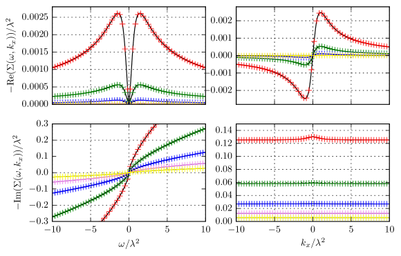
Figure 2: Real and imaginary parts of the self energy obtained using the large-$k_{F}$ Landau-damped propagator. This plot shows the agreement between the numerics and the analytical solution, verifying that both solutions are correct. Notice the difference in magnitude between the real and imaginary part. The agreement of the real parts shows that the numerical procedure has a very small relative error. All plots are for the $k_{x},\omega=\lambda^{2}$ slice with $v=1$.

We can now show the problematic feature. Recall that Eq. (19) is the Green’s function in Euclidean signature. Continuing to the imaginary line, $\omega=-i\omega_{R}$, this becomes the proper retarded Greens function, $G_{R}(\omega_{R},k_{x})$, and from this we can obtain the spectral function $A(\omega_{R},k_{x})=-2\mathrm{Im}\ G_{R}(\omega_{R},k_{x})$. As it encodes the excitation spectrum, the spectral function ought to be a positive function that moreover equals $2\pi$ when integrated over all energies $\omega_{R}$, for any momentum $k$. This large $M_{D}$ spectral function contains an oscillating singularity at $\omega_{R}=vk_{x}$. We are free to move the contour into complex $\omega_{R}$-plane by deforming $\omega_{R}\rightarrow\omega_{R}+i\Omega$ where $\Omega$ is positive but otherwise arbitrary. Upon doing this it is easy to numerically verify that indeed the integral over $\omega_{R}$ gives $2\pi$. However, if we look at the behaviour close to the essential singularity, the function oscillates rapidly and does not stay positive as one approaches the singularity; see Fig. 3. This reflects that the large $M_{D}$ approximation done in this way is not consistent. Even though the approximation for the exponent $I(\tau,r)\equiv\frac{\tilde{I}(\tau,r)}{(M_{D})^{2/3}}$ is valid to leading order in $1/M_{D}$, this is not systematic after exponentiation to obtain the fermion two-point function

$$\underset{M_{D}\rightarrow\infty}{G_{f}}(\tau,r)=\frac{1}{2\pi(ir-v\tau)}\exp\left(\frac{\tilde{I}(\tau,r)}{M_{D}^{2/3}}+\mathcal{O}\Big{(}\frac{1}{(M_{D})^{4/3}}\Big{)}\right).$$ (20)

Reexpanding the exponent one immediately sees that keeping only the leading term in $I(\tau,r)$ mixes at higher order with the subleading terms at lower order in $1/M_{D}$

$$\underset{M_{D}\rightarrow\infty}{G_{f}}(\tau,x)=\frac{1}{2\pi(ir-v\tau)}\left(1+\frac{\tilde{I}(\tau,r)}{M_{D}^{2/3}}+\mathcal{O}(M_{D}^{-4/3})+\frac{1}{2}\left(\frac{\tilde{I}(\tau,r)}{M_{D}^{2/3}}+\ldots\right)^{2}\right).$$ (21)

Despite this problematic feature, we will show from the exact result that in the IR $\underset{M_{D}\rightarrow\infty}{G_{f}}$ (with a small modification) does happen to capture the correct physics.

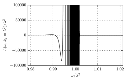
Figure 3: Exact fermion spectral function based on the large-$M_{D}$ approximation for the exact boson propagator. Notice that the function is not positive everywhere. Here $k=\lambda^{2}$, $v=1$ and $M_{D}=2\pi\lambda^{2}$.

IV.0.1 Exact fermion two-point function for large $k_{F}$ with $M_{D}$ fixed; $v=1$

We therefore make no further assumption regarding the value of $M_{D}$ and we return to the full integral Eq. (11) to determine the real space fermion two-point function. Solving this in general is difficult, and to simplify mildly we consider the special case $v=1$. In our previous studies of the quenched $M_{D}=0$ limit we saw that this choice for value of $v$ is actually not very special, even though it appears that there is an enhanced symmetry. In fact, nothing abruptly happens as $v\rightarrow 1$, except that the quenched $M_{D}=0$ solution can be written in closed form for this value of $v=1$. Nor for the case of large $M_{D}$ is the choice $v=1$ in any way special. As can be seen above in Eq. (16) for large $M_{D}$ all $v$ are equivalent up to a rescaling of $\tau$ versus $r$ and a rescaling of the single length scale $l_{0}$. We may therefore expect that for a finite $M_{D}$, the physics of $0<v<1$ is qualitatively the same as the (not-so-) special case $v=1$.

After setting $v=1$ and changing to spherical coordinates we have

$$I=\lambda^{2}\int\mathrm{d}\tilde{r}\mathrm{d}\phi\mathrm{d}\theta\mathrm{e}^{2i\phi}\frac{\cos\big{(}\tilde{r}\sin(\theta)(\tau\sin(\phi)-r\cos(\phi))\big{)}-1}{8\pi^{3}\sin(\theta)^{2}\big{(}M_{D}^{2}|\sin(\phi)|+\tilde{r}^{2}/\sin(\theta)\big{)}}~{}.$$ (22)

Performing the $\tilde{r}$ integral gives us

$$I=\pi^{4}\lambda^{2}\int\mathrm{d}\phi\mathrm{d}\theta\mathrm{e}^{2i\phi}\frac{\mathrm{e}^{-M_{D}|\tau\sin(\phi)-r\cos(\phi)|\sqrt{|\sin(\phi)|\sin(\theta)^{3}}}-1}{16M_{D}\sqrt{|\sin(\phi)|\sin(\theta)^{3}}}~{}.$$ (23)

Note that if the signs of both $\tau$ and $r$ are flipped, then this is invariant. Changing the sign of only $\tau$, and simultaneously making the change of variable $\phi\rightarrow-\phi$, then the (real) fraction is invariant but the exponent in the prefactor changes sign. Thus, $I$ goes to $I^{*}$ as the sign of either $\tau$ or $r$ is changed. Without loss of generality, we can assume that both of them are positive from now on. We further see that the integrand is invariant under $\phi\rightarrow\phi+\pi$, so we may limit the range of $\phi$ to $(0,\pi)$ by doubling the value of integrand. Similarly we limit $\theta$ to $(0,\pi/2)$ and multiply by another factor of 2. We then make the changes of variables:

$$\begin{split}\phi&=\tan^{-1}(s)+\pi/2\\ \theta&=\sin^{-1}(u^{2/3})\end{split}$$ (24)

with $s\in\mathbb{R}$ and $u$ is integrated over the range $(0,1)$. For convenience we introduce the function

$$z(s)=M_{D}|sr+\tau|(1+s^{2})^{-3/4}.$$ (25)

Now the two remaining integrals can be written as

$$I=\frac{\lambda^{2}}{M_{D}}\int\mathrm{d}s\mathrm{d}u\frac{(\mathrm{e}^{-uz(s)}-1)(s-i)}{6\pi^{2}(s+i)(1+s^{2})^{3/4}u^{4/3}\sqrt{(1-u^{4/3})}}.$$ (26)

After expanding the exponential we can perform the $u$ integral term by term. We are left with

$$I=\frac{\lambda^{2}}{M_{D}}\int\mathrm{d}s\sum_{n=1}^{\infty}\frac{(1+s^{2})^{1/4}(-z(s))^{n}}{8\pi^{3/2}n!(i+s)^{2}}\frac{\Gamma\Big{(}\frac{3n-1}{4}\Big{)}}{\Gamma\Big{(}\frac{3n+1}{4}\Big{)}}.$$ (27)

This can be resummed into a sum of generalized hypergeometric functions, but this is not useful at this stage. Instead we once again integrate term by term. Collecting the prefactors and introducing the constant $a=\tau/r$, the $n$-th term can be written as

$$I=\sum_{n=1}^{\infty}c_{n}\int\mathrm{d}s\,(s-i)^{2}|s+a|^{n}(1+s^{2})^{-(7+3n)/4}.$$ (28)

This can be written as

$$I=\sum_{n=1}^{\infty}c_{n}\int\mathrm{d}s\mathrm{d}w\,(s-i)^{2}|s+a|^{n}\frac{\mathrm{e}^{-w(s^{2}+1)}w^{3(1+n)/4}}{(3(1+n)/4)!},$$ (29)

where $w$ is integrated on $(0,\infty)$. After splitting the integral at $s=-a$ to get rid of the absolute value we can calculate the $s$ integrals in terms of confluent hypergeometric functions ${}_{1}F_{1}(a,b;z)$. Adding the two halves $s<-a$ and $s>-a$ of the integral we have

$$\begin{split}I=&\sum_{n=1}^{\infty}c_{n}\int\mathrm{d}w\frac{\Gamma\Big{(}\frac{1+n}{2}\Big{)}\mathrm{e}^{-(1+a^{2})w}}{2(3(1+n)/4)!}\Bigg{(}2w(i+a)^{2}\ _{1}F_{1}\Big{(}\frac{2+n}{2},\frac{1}{2};a^{2}w\Big{)}\\ &+(2+n)\ _{1}F_{1}\Big{(}\frac{4+n}{2},\frac{1}{2};a^{2}w\Big{)}-4aw(2+n)(i+a)\ _{1}F_{1}\Big{(}\frac{4+n}{2},\frac{3}{2};a^{2}w\Big{)}.\Bigg{)}\end{split}$$ (30)

It may look like we have just exchanged the $s$-integral for the $w$-integral, but by writing the hypergeometric functions in series form,

$$\begin{split}I=&\sum_{n=1}^{\infty}c_{n}\int\mathrm{d}w\sum_{m=0}^{\infty}\frac{2^{2m-1}a^{2m}\mathrm{e}^{-(1+a^{2})w}w^{\frac{n-3}{4}+m}\Gamma\Big{(}\frac{1+n}{2}+m\Big{)}}{\Gamma\Big{(}\frac{7+3n}{4}\Big{)}\Gamma\Big{(}2+2m\Big{)}}\times\\ &\times(n(1+2m-4a(i+a)w)+(1+2m)(1+2m-2(1+a^{2})w))~{},\end{split}$$ (31)

the $w$ integral can now be performed. The result is

$$\begin{split}I=\sum_{n=1,m=0}^{\infty}&c_{n}\frac{(a+i)4^{m-1}a^{2m}\left(a^{2}+1\right)^{-\frac{1}{4}(4m+n+5)}\Gamma\left(m+\frac{n+1}{4}\right)\Gamma\left(m+\frac{n+1}{2}\right)}{\Gamma(2m+2)\Gamma\left(\frac{7+3n}{4}\right)}\times\\ &\times\left(a\left(2m-6mn-2n^{2}-n+1\right)-i(2m+1)(n+1)\right).\end{split}$$ (32)

The sum over $m$ can be expressed in terms of the ordinary hypergeometric function, ${}_{2}F_{1}(a_{1},a_{2};b;z)$:

$$I=\sum_{n=1}^{\infty} c_{n}\frac{(n+1)\left(a^{2}+1\right)^{-\frac{n}{4}-\frac{1}{4}}\Gamma\left(\frac{n+1}{4}\right)\Gamma\left(\frac{n+1}{2}\right)}{24(a-i)^{2}(a+i)\Gamma\left(\frac{3n}{4}+\frac{7}{4}\right)}\times$$ (33)

$$\times\left(a^{2}(n+1)(-3an+a-i(n+1))\,_{2}F_{1}\Bigg{(}\frac{n+3}{2},\frac{n+5}{4};\frac{5}{2};\frac{a^{2}}{a^{2}+1}\right)+$$ (34)

$$-6\left(a^{2}+1\right)(a(2n-1)+i)\,_{2}F_{1}\left(\frac{n+1}{4},\frac{n+1}{2};\frac{3}{2};\frac{a^{2}}{a^{2}+1}\right)\Bigg{)}.$$ (35)

The space-time dependence in this expression is in $a=\tau/r$ and with additional $r$-dependence in the coefficients $c_{n}$ The result above is the value for both $\tau$ and $r$ positive. Using the known symmetries presented above, the solution can be extended to all values of $\tau$ and $r$ by appropriate absolute value signs. Then changing variables to

$$\begin{split}\tau&=R\cos(\Phi)\\ r&=R\sin(\Phi)\end{split}$$ (36)

we have

$$\begin{split}I=\frac{\lambda^{2}f\left(RM_{D},\Phi\right)}{M_{D}}\end{split}$$ (37)

with the function $f(\tilde{R},\Phi)$ given by

$$\begin{split}f(\tilde{R},\Phi)=&\sum_{n=1}^{\infty}f_{n}\tilde{R}^{n}\\ f_{n}=&\frac{e^{i\Phi}2^{-1-n}(-1)^{n}\Gamma\left(\frac{n+1}{4}\right)\left|\sin(\Phi)\right|^{\frac{1+3n}{2}}}{9\pi(3n-1)\Gamma\left(\frac{n}{2}+1\right)\Gamma\left(\frac{1+3n}{4}\right)}\cdot\\ &\cdot\Bigg{(}\,_{2}F_{1}\left(\frac{n+3}{2},\frac{n+5}{4};\frac{5}{2};\cos^{2}(\Phi)\right)(n+1)\cdot\\ &\ \ \ \ \ \ \cdot\cos^{2}(\Phi)((1-3n)\cos(\Phi)-i(n+1)\sin(\Phi))\\ &\ \ +\,_{2}F_{1}\left(\frac{n+1}{4},\frac{n+1}{2};\frac{3}{2};\cos^{2}(\Phi)\right)6((1-2n)\cos(\Phi)-i\sin(\Phi))\Bigg{)}.\end{split}$$ (38)

This exact infinite series expression for the exponent $I(\tilde{R},\Phi)$ gives us the exact fermion two-point function in real (Euclidean) space (time). We have not been able to find a closed form expression for this final series. Note that $f_{n}\sim 1/n!$ for large $n$, and the series therefore converges rapidly. Moreover, numerically the hypergeometric functions are readily evaluated to arbitrary precision (e.g. with Mathematica), and therefore the value of $f(\tilde{R},\Phi)$ can be robustly evaluated to any required precision.

As a check on this result, we can compare it to the exact result in the quenched $M_{D}=0$ limit in quenched , where the exact answer was found in a different way. In the limit where $M_{D}\rightarrow 0$ we see that only the first term of this series gives a contribution and the expression for the exponent collapses to

$$\lim_{M_{D}\rightarrow 0}I(R,\Phi)=\lambda^{2}f_{1}R=\lambda^{2}\frac{e^{2i\Phi}}{12\pi}R.$$ (39)

In Cartesian coordinates this equals

$$\lim_{M_{D}\rightarrow 0}I(\tau,r)=\lambda^{2}\frac{(\tau+ir)^{2}}{12\pi\sqrt{\tau^{2}+r^{2}}}.$$ (40)

This is the exact same expression as found in quenched for $v=1$.

There is one value of the argument for which $f(\tilde{R},\Phi)$ drastically simplifies. For $r=0$ ($\Phi=0,\pi$) we have

$$\begin{split}f_{n}(\Phi=0)=&-\frac{(-1)^{n}}{6\pi\Gamma(n+2)}\end{split}$$ (41)

and thus

$$\begin{split}f(\tilde{R},\Phi=0)=&\frac{1}{6\pi}+\frac{e^{-\tilde{R}}-1}{6\pi\tilde{R}}.\end{split}$$ (42)

Further numerical analysis shows that the real part of $f(\tau,r)$ is maximal for $r=0$.

IV.0.2 The IR limit of the exact fermion two-point function compared to the large-$M_{D}$ expansion

With this exact real space answer, we can now reconsider why the large $M_{D}$ (large $N_{f}k_{F}$) limit fails and which expression does reliably capture the strongly coupled IR physics of interest. The expression obtained above, Eq. (38), is not very useful for extracting the IR Green’s function or the Green’s function at a large $M_{D}$ as the expression is organized in an expansion around $RM_{D}=0$. To study the limit where $RM_{D}\gg 1$ we can go back to Eq. (26). With this expression we see that the exponential in the integrand, $e^{-uz(s)}$ with $z\sim M_{D}|sr+\tau|\sim\tilde{r}$, is generically suppressed for large $\tilde{R}=RM_{D}$. The exceptions are when either $sr+\tau$ is small, $s$ is large, or $u$ is small. The first two cases are also unimportant in the $\tilde{R}\gg 1$ limit. In the first case we restrict the $s$ integral to a small range of order $1/\tilde{R}$ around $-\tau/r$; this contribution therefore becomes more and more negligible in the limit $\tilde{R}\gg 1$. In the second case we will have a remaining large denominator in $s$ outside the exponent that also suppresses the overall integral. Thus for large $\tilde{R}$, the only appreciable contribution of the exponential term to the integral in $I(\tau,r)$ arises when $u$ is small. To use this, we first write the integral as

$$I_{\mathrm{IR}} =I_{\mathrm{IR,exp}}+I_{\mathrm{IR},-1},$$ (43)

$$I_{\mathrm{IR,exp}}(\tau,r) =\lambda^{2}\int_{-\infty}^{\infty}\mathrm{d}s\!\frac{s-i}{6\pi^{2}(s+i)(1+s^{2})^{3/4}M_{D}}\left(\int_{0}^{1}\mathrm{d}u\frac{\mathrm{e}^{-4uz(s)}-1}{u^{4/3}\sqrt{1-u^{4/3}}}-\int_{1}^{\infty}\mathrm{d}u\frac{1}{u^{4/3}}\right)$$

$$\simeq\lambda^{2}\int_{-\infty}^{\infty}\mathrm{d}s\!\frac{s-i}{6\pi^{2}(s+i)(1+s^{2})^{3/4}M_{D}}\left(\int_{0}^{1}\mathrm{d}u\frac{\mathrm{e}^{-4uz(s)}-1}{u^{4/3}}-\int_{1}^{\infty}\mathrm{d}u\frac{1}{u^{4/3}}\right),$$

$$I_{\mathrm{IR,-1}}(\tau,r) =\lambda^{2}\int_{-\infty}^{\infty}\mathrm{d}s\!\frac{s-i}{6\pi^{2}(s+i)(1+s^{2})^{3/4}M_{D}}\left(\int_{1}^{\infty}\mathrm{d}u\frac{1}{u^{4/3}}+\int_{0}^{1}\mathrm{d}u\left(\frac{-u^{-4/3}}{\sqrt{1-u^{4/3}}}+u^{-4/3}\right)\right).$$

We have added and subtracted an extra term to each to ensure convergence of each of the separate terms. Since the important contribution to $I_{\mathrm{IR,exp}}$ is from the small $u$ region we can extend its range from (0,1) to $(0,\infty)$. This way, the integrals can then be done

$$I_{\mathrm{IR},\mathrm{exp}} =\int_{-\infty}^{\infty}\mathrm{d}s\frac{-\lambda^{2}\left|sr+\tau\right|^{1/3}}{3^{3/2}\pi M_{D}^{2/3}(s+i)^{2}\Gamma\left(\frac{4}{3}\right)}$$

$$=-\frac{\Gamma\left(\frac{2}{3}\right)\lambda^{2}\left|r\right|^{1/3}}{3^{3/2}\pi M_{D}^{2/3}\left(1+\frac{i\tau}{r}\right)^{2/3}},$$ (44)

$$I_{\mathrm{IR},-1} =\int_{-\infty}^{\infty}\mathrm{d}s\frac{\lambda^{2}(s-i)}{6\pi^{2}(s+i)(1+s^{2})^{3/4}M_{D}}\Bigg{(}\int_{0}^{\infty}\mathrm{d}u\Big{(}\frac{1}{u^{4/3}}-\frac{\theta(1-u)}{u^{4/3}\sqrt{1-u^{4/3}}}\Big{)}\Bigg{)}$$

$$=\frac{\lambda^{2}}{6\pi M_{D}}.$$ (45)

In total we have for large $\tilde{R}$:

$$I=-\frac{\Gamma\left(\frac{2}{3}\right)\lambda^{2}\left|r\right|}{3^{3/2}\pi M_{D}^{2/3}\left(|r|+i\operatorname{sgn}(r)\tau\right)^{2/3}}+\frac{\lambda^{2}}{6\pi M_{D}}+\mathcal{O}(\lambda^{2}M_{D}^{-4/3}R^{-1/3}).$$ (46)

We see that the leading order term in $R$ is the same as was obtained from the large $M_{D}$ approximation of the exponent. The first subleading term is just a constant. This is good news because we already have the Fourier transform of this expression. This result is valid for length scales larger than $1/M_{D}$ with a bounded error of the order $R^{-1/3}$. Defining this approximation as $G_{\mathrm{IR}}$, i.e.

$$G_{\mathrm{IR}}=G_{0}\exp\left(-\frac{\Gamma\left(\frac{2}{3}\right)\lambda^{2}\left|r\right|}{3^{3/2}\pi M_{D}^{2/3}\left(|r|+i\operatorname{sgn}(r)\tau\right)^{2/3}}+\frac{\lambda}{6\pi M_{D}}\right)~{},$$ (47)

the error of this approximation follows from:

$$\Delta G_{\mathrm{IR}}=G-G_{\mathrm{IR}}=G_{\mathrm{IR}}\left(\exp\left(\mathcal{O}(\tilde{R}^{-1/3})\right)-1\right).$$ (48)

Since the exponential in $G_{\mathrm{IR}}$ is bounded we have that $\Delta G_{\mathrm{IR}}=\mathcal{O}(r^{-4/3})$. After Fourier transforming this translates to an error of order $\mathcal{O}(k^{-2/3})$.

IV.1 The exact fermion two-point function in momentum space: Numerical method

Having understood the shortcomings of the naive large $M_{D}$ answer, the way to derive the exact answer in real space, and the correct IR approximation, we can now analyze the behavior of the quantum critical metal at low energies. For this we need to transform to frequency-momentum space. As our exact answer is in the form of an infinite sum, this is not feasible analytically. We therefore resort to a straightforward numerical Fourier analysis.

To do so we first numerically determine the real space value of the exact Green’s functions. To do so accurately, several observations are relevant

• The coefficients $f_{n}$ in the infinite sum for $I(\tau,r)$ decay factorially in $n$ so once $n$ is of order $\tilde{R}$, convergence is very rapid.

• The hypergeometric functions for each $n$ are costly to compute with high precision, but with the above choice of polar coordinates the arguments of the hypergeometric functions are independent of $R$ and $M_{D}$. We therefore numerically evaluate the series over a grid in $\tilde{R}$ and $\Phi$. We can then reuse the hypergeometric function evaluations many times and greatly decrease computing time.

• The real space polar grid will be limited to a finite size. The IR expansion from Eq. (47) can be used instead of the exact series for large enough $\tilde{R}$. To do so, we have to ensure an overlapping regime of validity. It turns out that a rather large value of $\tilde{R}$ is necessary to obtain numerical agreement between these two expansions, i.e. one needs to evaluate a comparably large number of terms in the expansion. For the results presented in this paper it has been necessary to compute coefficients up to order 16 000 in $\tilde{R}$, for many different angles $\Phi$. The function is bounded for large $\tau$ and $\tilde{R}$ but each term grows quickly. This means that there are large cancellations between the terms that in the end give us a small value. We therefore need to calculate these coefficients to very high precision in evaluating the polynomial. For these high precision calculations, we have used the Gnu Multiprecision Library GMP .

• On this polar grid we computed the exact answer for $\tilde{R}<\tilde{R}_{0}\approx 1000$ and used cubic interpolation for intermediate values. For larger $\tilde{R}$ we use the asymptotic expansion in Eq. (47).

We then use a standard discrete numerical Fourier transform (DFT) to obtain the momentum space two-point function from this numeric prescription for $G(R,\Phi)$. Sampling $G(R,\Phi)$ at a finite number of discrete points, the size of the sampling grid will introduce an IR cut-off at the largest scales we sample and a UV-cut off set by the smallest spacing between points. These errors in the final result can be minimized by using the known asymptotic values analytically. Rather than Fourier transforming $G(\tau,r)$ as a whole, we Fourier transform $G_{\mathrm{diff}}(\tau,r)=G(\tau,r)-G_{\mathrm{IR}}(\tau,r)$ instead. Since both these functions approach the free propagator in the UV, the Fourier transform of its difference will decay faster for large $\omega$ and $k$. This greatly reduces the UV artefacts inherent in a discrete Fourier transform. These two functions also approach each other for large $\tau$ and $x$. In fact, with the numerical method we use to approximate $f(\tilde{R},\Phi)$ described above, they will be identical for $\tilde{R}_{0}<M_{D}\sqrt{\tau^{2}+r^{2}}$. This means that we only need to sample the DFT within that area. With a DFT we will always get some of the UV tails of the function that gives rise to folding aliasing artefacts. Now our function decays rapidly so one could do a DFT to very high frequencies and discard the high frequency part. This unfortunately takes up a lot of memory so we have gone with a more CPU intensive but memory friendly approach. To address this we perform a convolution with a Gaussian kernel, perform the DFT, keep the lowest 1/3 of the frequencies and then divide by the Fourier transform of the kernel used. This gives us a good numeric value for $G_{\mathrm{diff}}(\omega,k)$. To this we add our analytic expression for $G_{\mathrm{IR}}(\omega,k)$.

V The physics of 2+1 quantum critical metals in double scaling limit

With the exact real space expression and the numerical momentum space solution for the full non-perturbative fermion Green’s function, we can now discuss the physics of the elementary quantum critical metal in the double scaling limit. Let us emphasize right away that all our results are in Euclidean space. Although a Euclidean momentum space Green’s function can be used to find a good Lorentzian continuation with a well-defined and consistent spectral function, this function is not easily obtainable from our numerical Euclidean result. We leave this for future work. The Euclidean signature Green’s function does not visually encode the spectrum directly, but for very low energies/frequencies the Euclidean and the Lorentzian expressions are nearly identical, and we can extract much of the IR physics already from the Euclidean correlation function.

In Fig. 4 we show density plots of the imaginary part of $G(\omega,k_{x})$ for different values of $M_{D}$ as well as cross-sections at fixed low $\omega$. For the formal limit $M_{D}=0$ we detect three singularities near $\omega=0$ corresponding with the three Fermi surfaces found in Lorentzian signature in our earlier work quenched . However, for any appreciable value of the dimensionless ratio $M_{D}/\lambda^{2}$ one only sees a single singularity. As the plots for $G(\omega,k_{x})$ at low frequency show, its shape approaches that of the strongly Landau-damped $M_{D}\rightarrow\infty$ result, Eq. (19), as one increases $M_{D}/\lambda^{2}$, though for low $M_{D}$ it is still distinguishably different. Recall that our results are derived in the limit of large $k_{F}$ and therefore a realistic ($N_{f}\sim 1$) value for $M_{D}$ is $M_{D}\sim\lambda\sqrt{N_{f}k_{F}}\gg\lambda^{2}$.

(A)
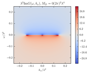
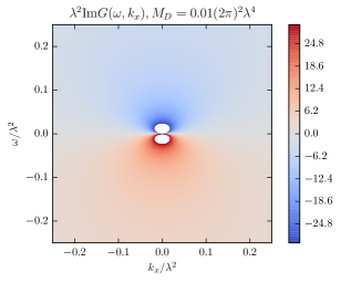
(B)

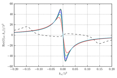
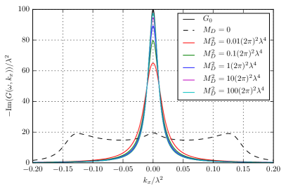
Figure 4: (A) Density plots of the imaginary part of the exact (Euclidean) fermion Green’s function $G(\omega,k_{x})$ for various values of $M_{D}$. In the quenched limit $M_{D}=0$ the three Fermi surface singularities are visible. For any appreciable finite $M_{D}$ the Euclidean Green’s function behaves as a single Fermi surface non-Fermi liquid. (B) Real and imaginary parts of $G(\omega,k_{x})$ for very small $\omega=0.01\lambda^{2}$.

This result is in contradistinction to what happens to the bosons. When the bosons are not affected in the IR, i.e. the quenched limit, the fermions are greatly affected by the boson: there is a topological Fermi surface transition and the low-energy spectrum behaves as critical excitations quenched . However, once we increase $M_{D}$ to realistic values, the bosonic excitations are rapidly dominated in the IR by Landau damping but we now see that this reduces the corrections to the fermions. As $M_{D}$ is increased for fixed $\omega$, $k_{x}$, the deep IR fermion two-point function approaches more and more that of the simple RPA result with self-energy $\Sigma\sim i\omega^{2/3}$.

A more careful analysis of the IR reveals that there are several distinct $\omega\rightarrow 0$ limits of the two-point function:

$$\lim_{\begin{subarray}{c}\omega\rightarrow 0,\\ k_{x}\text{ fixed}\end{subarray}}G_{\mathrm{IR}}(\omega,k_{x}) \approx\mathrm{e}^{\frac{\lambda^{2}}{6\pi M_{D}}}\frac{1}{i\omega-k_{x}-\Sigma_{\mathrm{RPA}}}$$

$$\lim_{\begin{subarray}{c}\omega\rightarrow 0,\\ k_{x}/\omega\text{ fixed}\end{subarray}}G_{\mathrm{IR}}(\omega,k_{x}) \approx\mathrm{e}^{\frac{\lambda^{2}}{6\pi M_{D}}}\frac{1}{i\omega-k_{x}-\frac{4\pi}{3\sqrt{3}}\Sigma_{\mathrm{RPA}}}$$

However in the case of $\omega^{2}\sim l_{0}k_{x}^{3}$, the full expression for $G_{\mathrm{IR}}$ is necessary to describe the low energy limit,

$$\begin{split}\lim_{\begin{subarray}{c}\omega\rightarrow 0,\\ l_{0}k_{x}^{3}\omega^{-2}\text{ fixed}\end{subarray}}G_{\mathrm{IR}}(\omega,k_{x})=\mathrm{e}^{\frac{\lambda^{2}}{6\pi M_{D}}}\Bigg{[}&\frac{1}{i\omega-k_{x}}\cos\left(\frac{\omega}{l_{0}^{1/2}(\omega+ik_{x})^{3/2}}\right)\\ &+\frac{6\sqrt{3}i\Gamma\left(\frac{1}{3}\right)\omega^{2/3}}{8\pi l_{0}^{1/3}(\omega+ik_{x})^{2}}\,_{1}F_{2}\left(1;\frac{5}{6},\frac{4}{3};-\frac{\omega^{2}}{4l_{0}(\omega+ik_{x})^{3}}\right)+\\ &+\frac{3\sqrt{3}i\Gamma\left(-\frac{1}{3}\right)\omega^{4/3}}{8\pi l_{0}^{2/3}(\omega+ik_{x})^{3}}\,_{1}F_{2}\left(1;\frac{7}{6},\frac{5}{3};-\frac{\omega^{2}}{4l_{0}(\omega+ik_{x})^{3}}\right)\Bigg{]},\end{split}$$ (49)

This existence of multiple limits shows in fact that the RPA result is never a good low energy (less than $M_{D}$) approximation for any value of $M_{D}/\lambda^{2}$. We can illustrate this more clearly by studying the self-energy of the fermion $\Sigma(\omega,k_{x})=G(\omega,k_{x})^{-1}-G_{0}(\omega,k_{x})^{-1}$. It is shown in Fig. 5 that the naive large $M_{D}$ RPA result (dotted lines) does agree for large $M_{D}$ at $\omega=0,k_{x}=0$ and the leading $\omega$ dependence of the imaginary part is captured. The leading $k_{x}$ dependence is not captured by RPA. On the other hand, our improved approximation for the low energy regime $G_{\mathrm{IR}}$ (dashed lines) captures these higher order terms in the low energy expansion of $G(\omega,k_{x})$ very well and also works for finite values of $M_{D}/\lambda^{2}$.

(A)
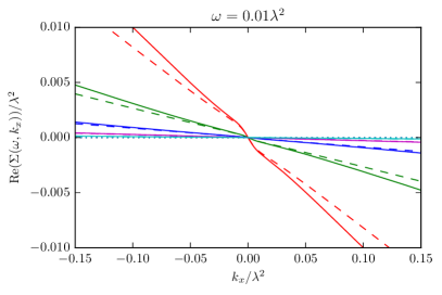
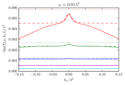
(B)

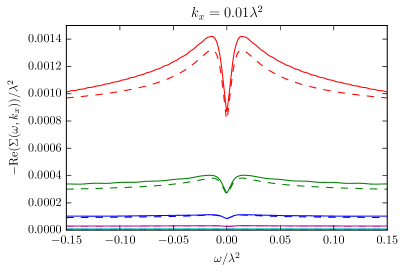
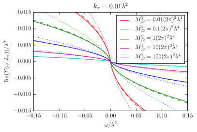
Figure 5: Real and imaginary parts of the fermion self-energy for (A) $\omega=0.01\lambda^{2}$ and for (B) $k_{x}=0.01\lambda^{2}$. Dashed lines show the $G_{\mathrm{IR}}$-approximation; dotted lines show the RPA result.

In all cases it is clear that the Fermion excitation, though qualitatively sharp, is not a Fermi liquid quasiparticle. We can calculate the occupation number and check whether it is consistent with the non-Fermi liquid nature of the Green’s function. With a Fermi liquid by definition is meant a spectrum with a discontinuity in the zero-temperature momentum distribution function $n_{k}=\int_{-\infty}^{0}\mathrm{d}\omega_{R}A(\omega_{R},k_{x})/2\pi$ with $A(\omega_{R},k_{x})$ the spectral function. As the spectral function is the imaginary part of the retarded Green’s functions and the latter is analytic in the upper half plane of $\omega_{R}$ we can move this contour to Euclidean $\omega$ and use the fact that $G(\omega,k_{x})$ approaches $G_{0}(\omega,k_{x})$ in the UV to calculate the momentum distribution function from our Euclidean results. In detail

$$n_{k_{x}}=-\int_{-\infty}^{0}\mathrm{d}\omega_{R}\mathrm{Im}\frac{G_{R}(\omega_{R},k_{x})}{\pi}=\mathrm{Im}\left[\int_{0}^{\Lambda}\mathrm{d}\omega i\frac{G(\omega,k_{x})}{\pi}+\int_{C}\mathrm{d}zi\frac{G(z,k_{x})}{\pi}\right]~{};$$ (50)

the first integral can be done with the numerics developed in the preceding section. The contour $C$ goes from $\Lambda$ to $-\infty$ and for large enough $\Lambda$ this is in the UV and can well be approximated by the free propagator. The resulting momentum distribution $n(k)$ is shown in Fig. 6. Within our numerical resolution, these curves are continuous as opposed to a Fermi liquid. This is of course expected; the continuity reflects the absence of a clear pole in the IR expansions in the preceding subsection. Note also that as $M_{D}$ is lowered, the finite $M_{D}$ curves approach the quenched result for $|k_{x}|>k_{x}^{*}$ where $k_{x}^{*}$ is the point of the discontinuity of the derivative of the quenched occupation number. At $k^{\ast}$ the (derivative) of the quenched momentum distribution number does have a discontinuity (reflecting the branch cut found in quenched ).

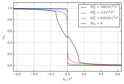
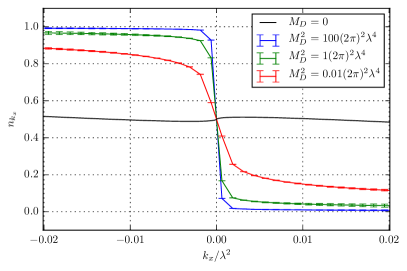
Figure 6: Momentum distribution function. The two plots show the same function for different ranges. The error bars of the lower figure show an estimate of the error due to using the free Green’s function close to the UV. The error-bars are exaggerated by a factor 100.

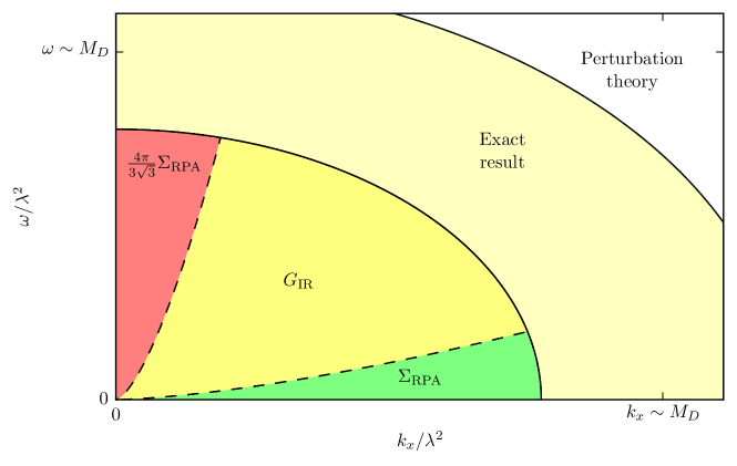
Figure 7: A sketch of the regimes of applicability of various approximations to the exact fermion Green’s function of the elementary quantum critical metal in the double scaling limit. The $G_{\mathrm{IR}}$

approximation is applicable both in the deep yellow region and the red and green regions.

VI Conclusion

We have presented a non-perturbative answer for the (Euclidean) fermion and boson two-point functions of the elementary quantum critical metal in the double limit of small $N_{f}$ and large $k_{F}$ with $N_{f}k_{F}$ fixed. This limit was taken order by order in perturbation theory and additionally before performing bosonic momentum integrals.

Our exact results clarify how approximations that have been made in the past hang together. The $N_{f}\rightarrow 0$, $k_{F}\rightarrow\infty$ theory is characterized by two energy scales $\lambda^{2}$ and $M_{D}$. For very large $\omega/\lambda^{2}$ and $\omega/M_{D}^{2}$ one can use perturbation theory in $\lambda$ to understand the theory. This is the perturbation around the UV-fixed point of a free fermion plus a free boson. In the deep IR region, $\omega\ll M_{D}^{2}$, we have an analytic expression for the two-point function, $G_{\mathrm{IR}}$. This shows a $\omega^{2}\sim l_{0}k_{x}^{3}$ scaling.

In the intermediate regime, the full numerical results that we have presented are necessary.

The quenched result we obtained earlier quenched does not seem to have a useful regime of validity. As the momentum occupation number $n(k)$ indicates, its precise regime of applicability depends discontinuously on the momentum $k/\lambda^{2}$. The discontinuity is surprising, but it can be explained analytically as an order of limits ambiguity. Although it is hard to capture the deep IR region for very small $N_{f}$ in the full numerics we find from $G_{\mathrm{IR}}$ that in the $\omega$-$k$ plane there is a region where the limit $N_{f}\rightarrow 0$ and $\omega,k_{x}\rightarrow 0$ do not commute. We show an indication of this in appendix C. Thus for scales below $\lambda^{2}$, the quenched result is not useful. For scales above $\lambda^{2}$ with $M_{D}$ small, we can use perturbation theory so also in this regime the quenched result is not useful. For small $\omega$ and $k_{x}$, below $M_{D}$, the IR approximation we presented above gives a good description of the physics. We have presented a pictorial overview of how the various approximations are related in Fig. 7.

As argued before the spectrum of the elementary quantum critical metal in the ordered double scaling limit obtained here is not the definitive one. Taking this limit after the bosonic integrals and the perturbative sum may give a different result. Another estimate for the true IR spectrum of the elementary quantum critical metal has been postulated before based on large $N_{f}$ approximations ChubukovNew ; SungSik1 ; Mross:2010rd , but our result at small $N_{f}$ gives a different IR. Our non-perturbative answer follows from the insight that in the limit of large $k_{F}$ all fermion loops with more than two external boson legs have cancellations upon symmetrization such that their scaling in $k_{F}$ is reduced. This higher loop cancellation has been previously put forward as a result of the strong forward scattering approximation. This approximation is engineered such that the Schwinger-Dyson equations combined with the fermion number Ward identity collapse to a closed set of equations. The solution to this closed set is the same dressed fermion correlator that we have presented. However the exact connection between the strong forward scattering approximation and the double scaling limit, is not clear. In the double scaling limit here, it is manifest that only the boson propagator is corrected and this in turn implies that the exact fermion Green’s function in real space is an exponentially dressed version of the free Green’s function.

At the physics level, an obvious next step is therefore to explore the spectrum of the elementary quantum critical metal including corrections in $N_{f}$ that are not proportional to $k_{f}$. Since this necessarily involves higher-point boson correlations, the role of self-interactions of the boson needs to be considered. These are also relevant in the IR and may therefore give rise to qualitatively very different physics than found here. We leave this for future work.

Appendix A Multiloop cancellation

The robustness of the one-loop result in case of linear fermionic dispersion was recognized before under the name of multiloop cancellation Metzner97 . The technical result is that for a theory with a simple Yukawa coupling and linear dispersion around a Fermi surface, a symmetrized fermion loop with more than two fermion lines vanishes. In our context the linear dispersion is a consequence of the large $k_{F}$ limit. In other words all higher loop contributions to the polarization $\Pi$ should be subleading in $1/k_{F}$. This was explicitly demonstrated at two loops in Kim2loop .

We will give here a short derivation of this multiloop cancellation in the limit $k_{F}\rightarrow\infty$. We may assume in this limit that the momentum transfer at any fermion interaction is always much smaller than the size of the initial ($\vec{k}$) and final momenta ($\vec{k}^{\prime}$) which are of the order of the Fermi momentum, i.e. $|\vec{k}^{\prime}-\vec{k}|\ll k_{F}$ with $|\vec{k}|,|\vec{k}^{\prime}|\sim k_{F}$. The free fermion Green’s function then reflects a linear dispersion

$$G_{0}(\omega,k)=\frac{1}{i\omega-vk}$$ (51)

We now Fourier transform back to real space, as multiloop cancellation is most easily shown in this basis. The real space transform of the “linear” free fermion propagator above is

$$G_{0}\left(\tau,r\right)=-\frac{i}{2\pi}\frac{\operatorname{sgn}(v)}{r+iv\tau},$$ (52)

where as before $r$ is the conjugate variable to $k=|\vec{k}|-k_{F}$. The essential step in the proof is that real space Green’s function manifestly obeys the identity quenched

$$G_{0}\left(z_{1}\right)G_{0}\left(z_{2}\right)=G_{0}\left(z_{1}+z_{2}\right)\left(G_{0}\left(z_{1}\right)+G_{0}\left(z_{2}\right)\right)$$ (53)

with $z\equiv r+iv\tau$. Consider then (the subpart of any correlation function/Feynman diagram containing) a fermion loop with $n\geq 2$ vertices along the loop connected to indistinguishable scalars (i.e. no derivative interactions and all interactions are symmetrized). The corresponding algebraic expression in a real space basis will then contain the expression

$$F\left(z_{1},...,z_{n}\right)=\sum_{(i_{1},..,i_{n})\in S_{n}}G_{0}\left(z_{i_{1}}-z_{i_{2}}\right)G_{0}\left(z_{i_{2}}-z_{i_{3}}\right)...G_{0}\left(z_{i_{n-1}}-z_{i_{n}}\right)G_{0}\left(z_{i_{n}}-z_{i_{1}}\right),$$ (54)

where $S_{n}$ is the set of permutations of the numbers 1 through $n$. Using the “linear dispersion” identity Eq. (53) and the shorthand notation $G_{0}\left(z_{i_{1}}-z_{i_{2}}\right)=G_{12}$ we obtain

$$F\left(z_{1},...,z_{n}\right)=\sum_{(i_{1},..,i_{n})\in S_{n}}G_{12}G_{23}...G_{n-1,1}\left(G_{n-1,n}+G_{n,1}\right).$$ (55)

Next we cyclically permute the indices from $1$ to $n-1$: $1\rightarrow 2$, $2\rightarrow 3$, …, $n-1\rightarrow 1$ in the sum

$$\sum_{(i_{1},..,i_{n})\in S_{n}}G_{12}G_{23}...G_{n-1,1}G_{n-1,n}=\sum_{(i_{1},..,i_{n})\in S_{n}}G_{23}G_{34}...G_{12}G_{1,n}.$$ (56)

This gives us

$$F\left(z_{1},...,z_{n}\right)=\sum_{(i_{1},..,i_{n})\in S_{n}}G_{12}G_{23}...G_{n-1,1}\left(G_{1,n}+G_{n,1}\right).$$ (57)

Then since $G_{i,j}$ corresponds to a (spinless) fermionic Green’s function, it is antisymmetric $G_{i,j}=-G_{j,i}$, and we can conclude that $F$ vanishes for $n\geq 3$. For $n=2$ it is not possible to use the identity Eq. (53) since we would need to evaluate $G(0)$ which is infinite.

Appendix B The Fourier transform of the fermion Green’s function in the large $M_{D}$ approximation

We will now show how to perform this Fourier transform. We need to calculate the following integral:

$$\underset{M_{D}\rightarrow\infty}{G_{f}}(\omega,k)=\int\mathrm{d}\tau\mathrm{d}x\frac{\mathrm{e}^{i(\omega\tau-kx)}}{2\pi(ix-v\tau)}\exp\left(-\frac{\left|x\right|}{l_{0}^{1/3}\left(\left|x\right|+iv\operatorname{sgn}(x)\tau\right)^{2/3}}\right)$$ (58)

First we note that integrand is $\tau$-analytic in the region $\{\tau\in\mathbb{C}:\min(0,vx)<\mathrm{Im}(\tau)<\max(0,vx)\}$. Since the integrand necessarily goes to 0 at $\infty$ we can thus shift the $\tau$ contour, $\tau\rightarrow\tau+ix/v$. We now have

$$\underset{M_{D}\rightarrow\infty}{G_{f}}(\omega,k)=-\int\frac{\mathrm{d}\tau\mathrm{d}x}{2\pi v\tau}\exp\left(i\omega\tau-x\left(ik+\omega/v+\frac{\operatorname{sgn}(x)}{l_{0}^{1/3}\left(iv\operatorname{sgn}(x)\tau\right)^{2/3}}\right)\right)$$ (59)

We have allowed ourselves to choose the order of integration, shift the contour, and then change the order. We see that the $x$ integral now is trivial but only converges for

$$-\frac{v^{1/3}}{2l_{0}^{1/3}|\tau|^{2/3}}<\mathrm{Re}(\omega)<\frac{v^{1/3}}{2l_{0}^{1/3}|\tau|^{2/3}}$$ (60)

This is fine since we know that the final result is $\omega$-analytic in both the right and left open half-planes. As long as we can obtain an answer valid within open subsets of both of these sets we can analytically continue the found solution to the whole half planes. We thus proceed assuming $\mathrm{Re}(\omega)$ is in this range. One can further use symmetries of our expression to relate the left and right $\omega$-half-planes, so to simplify matters, from now on we additionally assume $\omega$ to be positive. Let us now consider a negative $x$, we then see that the $\tau$ integral can be closed in the upper half plane and since it is holomorphic there the result will be 0. We can thus limit the $x$ integrals to $\mathbb{R}^{+}$. We then have

$$\underset{`N_{f}k_{F}\rightarrow\infty}{G_{f}}(\omega,k)=\int\mathrm{d}\tau\frac{\mathrm{e}^{i\omega\tau}}{2\pi v\tau}\frac{-1}{a+\frac{1}{l_{0}^{1/3}\left(iv\tau\right)^{2/3}}}$$ (61)

where $a=ik+\omega/v$. The integrand has a pole at $\left(i\tau\right)^{2/3}=-1/(al_{0}^{1/3}v^{2/3})$. Now break the integral in positive and negative $\tau$ and write it as

$$\underset{M_{D}\rightarrow\infty}{G_{f}}(\omega,k)=\frac{h((-i)^{2/3}u_{0}^{*})^{*}-h((-i)^{2/3}u_{0})}{2\pi va}$$ (62)

where

$$\begin{split}h(u)&=\int_{0}^{\infty}\mathrm{d}\tau\frac{\mathrm{e}^{i\tau}}{\tau+u\tau^{1/3}},\\ u_{0}&=\frac{\omega^{2/3}}{al_{0}^{1/3}v^{2/3}}.\end{split}$$ (63)

Usng Morera’s theorem we can prove that $h$ is holomorphic on $\mathbb{C}/\mathbb{R}^{-}$. Consider any closed curve $C$ in $\mathbb{C}/\mathbb{R}^{-}$. We need to show that

$$\int_{C}\mathrm{d}uh(u)=0$$ (64)

We do this by rotating the contour slightly counter clockwise. For any curve $C$ there is clearly a small $\epsilon>0$ such that we will still not hit the pole $\tau+u\tau^{1/3}=0$.

$$\int_{C}\mathrm{d}u\int_{0}^{(1+i\epsilon)\infty}\mathrm{d}\tau\frac{\mathrm{e}^{i\tau}}{\tau+u\tau^{1/3}},$$ (65)

The piece at $\infty$ converges without the denominator and thus goes to 0. Since the integral now converges absolutely we can use Fubini’s theorem to change the orders of integration

$$\int_{0}^{(1+i\epsilon)\infty}\mathrm{d}\tau\int_{C}\mathrm{d}u\frac{\mathrm{e}^{i\tau}}{\tau+u\tau^{1/3}}=0$$ (66)

And since also the integrand is holomorphic on a connected open set containing $C$ the proof is finished.

The function $h$ can for $0<\mathrm{arg}(u)<2\pi/3$ be expressed as a Meijer G-function:

$$h(u)=\frac{3}{8\pi^{5/2}}G_{3,5}^{5,3}\left(\begin{array}[]{c}0,\frac{1}{3},\frac{2}{3}\\ 0,0,\frac{1}{3},\frac{1}{2},\frac{2}{3}\\ \end{array}\Bigg{|}-\frac{u^{3}}{4}\right)$$ (69)

The G-function has a branch cut at $\mathbb{R}^{-}$ and because of that we can not easily write $h(u)$ in terms of it since the argument $u$ appears cubed in the argument of the G-function and we know that $h$ is holomorphic on all of $\mathbb{C}/\mathbb{R}-$. We can however express $h$ as an analytic continuation of the G-function past this branch cut, onto the further sheets of its Riemann surface.

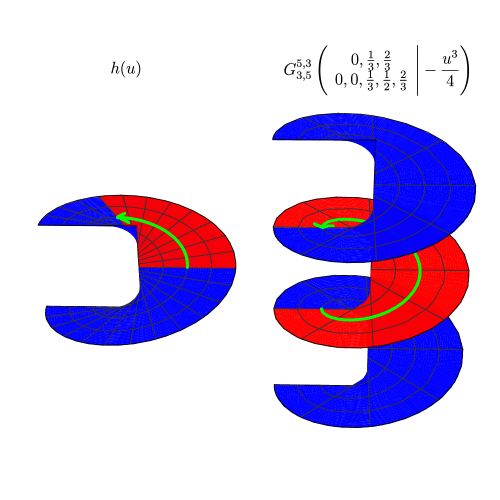
Figure 8: The left image shows part of the Riemann surface of the function $h$ and the right image shows part of the Riemann surface of the G-function. The part in red of the left image can be expressed as the G-function evaluated on its first sheet, the red part of the right image. The green arrow shows how points are mapped from one Riemann surface to the other by the mapping $u\mapsto-u^{3}/4$

We will write the G-function as a function with two real arguments, first the absolute value and second the phase of its otherwise complex argument. We will allow the phase to be any real number and when outside the range $[-\pi,\pi]$, we let the function be defined by its analytical continuation to the corresponding sheet. We hereafter omit the constant parameters of the G-function. We then have:

$$\begin{split}\underset{M_{D}\rightarrow\infty}{G_{f}}(\omega,k)&=3\frac{G_{3,5}^{5,3}\big{(}\frac{|u_{0}|^{3}}{4},-2\pi-3\arg(u_{0})\big{)}^{*}-G_{3,5}^{5,3}\big{(}\frac{|u_{0}|^{3}}{4},-2\pi+3\arg(u_{0})\big{)}}{16\pi^{7/2}va}\\ &=3\frac{G_{3,5}^{5,3}\big{(}\frac{|u_{0}|^{3}}{4},3\arg(u_{0})+2\pi\big{)}-G_{3,5}^{5,3}\big{(}\frac{|u_{0}|^{3}}{4},3\arg(u_{0})-2\pi\big{)}}{16\pi^{7/2}va}\end{split}$$ (70)

In the last step we used the fact that the G-function commutes with complex conjugation. We see that the Green’s function is given by a certain monodromy of the G-function. It is given by the difference in its value starting at a point $u_{0}^{3}/4$ on the sheet above the standard one and then analytically continuing clockwise around the origin twice to the sheet below the standard one and there return to $u_{0}^{3}/4$. Since we only need this difference, we might expect this to be a, in some sense, simpler function as would happen for e.g. monodromies of the logarithm. To see how to simplify this we look at the definition of the G-function. It is defined as an integral along $L$:

$$G_{p,q}^{\,m,n}\!\left(\left.\begin{matrix}a_{1},\dots,a_{p}\\ b_{1},\dots,b_{q}\end{matrix}\;\right|\,z\right)=\frac{1}{2\pi i}\int_{L}\frac{\prod_{j=1}^{m}\Gamma(b_{j}-s)\prod_{j=1}^{n}\Gamma(1-a_{j}+s)}{\prod_{j=m+1}^{q}\Gamma(1-b_{j}+s)\prod_{j=n+1}^{p}\Gamma(a_{j}-s)}\,z^{s}\,ds,$$ (71)

There are a few different options for $L$ and which one to use depends on the arguments. In our case $L$ starts and ends at $+\infty$ and circles all the poles of $\Gamma(b_{i}-s)$ in the negative direction. Using the residue theorem we can recast the integral to a series. We have double poles at all negative integers and some simple poles in between. The calculation to figure out the residues of all these single and double poles is a bit too technical to present here but in the end the series can be written as

$$\begin{split}G_{3,5}^{5,3}\left(z\right)=\sum_{n=0}^{\infty}\Big{(}a_{n}z^{n}+b_{n}z^{n}\log(z)+c_{n}z^{n+1/3}+d_{n}z^{n+1/2}+e_{n}z^{n+2/3}\Big{)}\end{split}$$ (72)

Now we perform the monodromy term by term and a lot of these terms cancel out.

$$\begin{split}&G_{3,5}^{5,3}\big{(}|z|,\arg(z)+2\pi\big{)}-G_{3,5}^{5,3}\big{(}|z|,\arg(z)-2\pi\big{)}=\\ &\sum_{n=0}^{\infty}\Big{(}4\pi ib_{n}z^{n}+i\sqrt{3}c_{n}z^{n+1/3}-i\sqrt{3}e_{n}z^{n+2/3}\Big{)}\end{split}$$ (73)

The coefficients $a_{i}$ contain both the harmonic numbers and the polygamma function whereas the other coefficients are just simple products of gamma functions. This simplification now lets us sum this series to a couple of generalized hypergeometric functions. Inserting the expressions for $a$ and $u_{0}$ we have

$$\begin{split}\underset{M_{D}\rightarrow\infty}{G_{f}}(\omega,k)=&\frac{1}{i\omega-kv}\cos\left(\frac{\omega}{vl_{0}^{1/2}(\omega/v+ik)^{3/2}}\right)\\ &+\frac{6\sqrt{3}i\Gamma\left(\frac{1}{3}\right)\omega^{2/3}}{8\pi l_{0}^{1/3}v^{5/3}(\omega/v+ik)^{2}}\,_{1}F_{2}\left(1;\frac{5}{6},\frac{4}{3};-\frac{\omega^{2}}{4l_{0}v^{2}(\omega/v+ik)^{3}}\right)+\\ &+\frac{3\sqrt{3}i\Gamma\left(-\frac{1}{3}\right)\omega^{4/3}}{8\pi l_{0}^{2/3}v^{7/3}(\omega/v+ik)^{3}}\,_{1}F_{2}\left(1;\frac{7}{6},\frac{5}{3};-\frac{\omega^{2}}{4l_{0}v^{2}(\omega/v+ik)^{3}}\right).\end{split}$$ (74)

Note that this expression is $\omega$-holomorphic for $\omega$ in the right half plane so our previous assumptions on $\omega$ can be relaxed as long as $\omega$ is in the right half plane. We note from expression (58) that if we change sign on both $\omega$ and $k$ and do the changes of variables $\tau\rightarrow-\tau$ and $x\rightarrow-x$ we end up with the same integral up to an overall minus sign. We can thus get the left half plane result using the relation

$$\underset{M_{D}\rightarrow\infty}{G_{f}}(-\omega,k)=-\underset{M_{D}\rightarrow\infty}{G_{f}}(\omega,-k).$$ (75)

As mentioned in the main text, this expression has been compared with numerics to verify that we have not made any mistakes. See Fig. 2. We have also done the two integrals for the Fourier transform in the opposite order, first obtaining a different Meijer G-function then using the G-function convolution theorem to do the second integral. In the end one obtains the same monodromy of the G-function as above. This expression can also be found in Appendix A.2 of ChubukovNew , however it was not entirely clear from the phrasing of the last paragraph that this function is actually the exact Fourier transform, Eq. (58).

Appendix C The discontinuous transition from the quenched to the Landau-damped regime

We show here why including Landau damping (finite $M_{D}$) physics starting from the quenched $N_{f}\rightarrow 0$ result, is discontinuous in the IR. To do so we calculate the Green’s function by imposing the $N_{f}\rightarrow 0$ limit from the begining. We need to evaluate the Fourier transform integral:

$$G_{L}\left(\omega,k\right)=\int_{-\infty}^{\infty}dx\int_{-L}^{L}d\tau G_{0}\exp\left(I_{0}+i\omega\cdot\tau-ik\cdot x\right),$$ (76)

where as before the free propagator is

$$G_{0}(\tau,x)=-\frac{i}{2\pi}\frac{1}{x+i\cdot\tau}$$ (77)

and the $N_{f}\rightarrow 0$ limit of the exponent of the real space Green’s function:

$$I_{0}=\frac{(\tau+i\cdot x)^{2}}{12\pi\sqrt{\tau^{2}+x^{2}}}.$$ (78)

Note however that the $\tau$ integral is divergent in this limit. Therefore in (76) we have introduced a cutoff $L$ in this direction. By looking at the full expansion of $I$ we can see that the natural value of $L$ is of the order $1/M_{D}$. For larger values of $\tau$ the asymptotic expansion describes $I$ better. We expect that for large enough momenta and frequencies the asymptotic region does not contribute to the Fourier transform and therefore the cutoff can be removed. This naive epxectation however is only partly true. We will shortly see that the region in the $\omega-k$ plane where the cutoff can be removed is more complicated and asymmetric in terms of the momenta and frequency.

Let us turn now to the evaluation of (76). After making the coordinate change $\tau\rightarrow\tau$, $x\rightarrow u\cdot\tau$ one of the integrals ($\tau$) can be evaluated analytically:

$$G_{L}\left(\omega,k\right)=\int_{-\infty}^{\infty}du\left(I_{1}(u)+I_{2}(u)+I_{3}(u)\right),$$ (79)

where

$$I_{1}(u)=\frac{6\exp\left(ikLu\sqrt{u^{2}+1}-iL\cdot\omega\cdot\sqrt{u^{2}+1}-\frac{L(u-i)^{2}}{12\pi}\right)}{12\pi(u+i)(ku-\omega)+i\sqrt{u^{2}+1}u+\sqrt{u^{2}+1}},$$ (80)

$$I_{2}(u)=\frac{6i\exp\left(-ikLu\sqrt{u^{2}+1}+iL\cdot\omega\cdot\sqrt{u^{2}+1}-\frac{L(u-i)^{2}}{12\pi}\right)}{12i\pi k(u+i)u+\sqrt{u^{2}+1}u-i\sqrt{u^{2}+1}+12\pi(1-iu)\omega},$$ (81)

$$I_{3}(u)=-\frac{144\pi(ku-\omega)}{u\left(-3+u\left(144\pi^{2}k^{2}(u+i)+u-3i\right)\right)-288\pi^{2}ku(u+i)\omega+144\pi^{2}(u+i)\omega^{2}+i}.$$ (82)

By numerically performing the single integral $u$ we can obtain $G_{M_{D}\rightarrow 0}$. Since it is easier than evaluating the Fourier transform of the true real-space version of the Green’s function it is worth understanding how the $L\rightarrow\infty$ (which is equivalent to $M_{D}\rightarrow 0$) works. The result is depicted on Fig. 9. In the shaded region (which corresponds to small $k$) the limit is not well defined while outside of this region the limit is equal to the quenched result. The numerics shows that for zero frequency, the edge of this region is at $k^{*}$, where the Green’s function is singular.

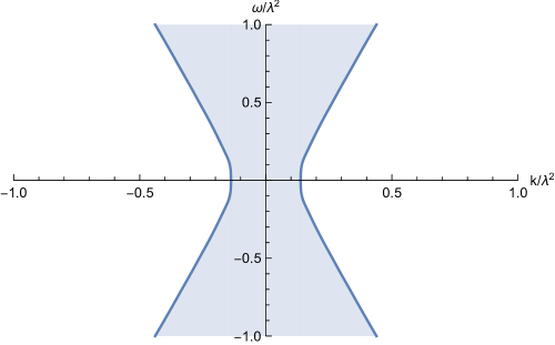
Figure 9: The region of convergence. In the shaded area the $L\rightarrow\infty$ ($N_{f}\rightarrow 0$) limit is not convergent while outside this area $\lim_{L\rightarrow\infty}G_{L}=G_{quenched}$.

We can qualitatively determine the line separating the convergent and divergent region. For this we assume that when $L$ is large one can expand the exponent in $u$

$$I_{1}(u)\sim\exp\left[u^{2}\left(-\frac{1}{12\pi}-\frac{1}{2}i\omega\right)L+\frac{iu(6\pi k+1)}{6\pi}L-iL\omega+\frac{L}{12\pi}+{\cal O}\left(L\dot{u^{3}}\right)\right].$$ (83)

We see that because of the term $-L\cdot u^{2}/(12\pi)$, the integrand is non-zero only in a narrow region around $u=0$. For the same reason we approximate the denominator of (80) by replace $u$ by zero there. With these simplifications we arrive to a gaussian integral which can be evaluated analytically:

$$\int_{-\infty}^{\infty}I_{1}(u)du\approx\frac{12i\sqrt{3}\pi\exp\left(\frac{iL\left(6\pi k^{2}+2k+\omega(-12\pi\omega+i)\right)}{12\pi\omega-2i}\right)}{(12\pi\omega+i)\sqrt{L(1+6i\pi\omega)}}.$$ (84)

The real part of (84) is

$$L\frac{3\left(\omega^{2}-k^{2}\right)\pi-k}{36\pi^{2}\omega^{2}+1}.$$ (85)

It is clear that if this value is positive (i.e. $3\left(\omega^{2}-k^{2}\right)\pi-k>0$) than the $L\rightarrow\infty$ limit is divergent. Looking at the numerical result in Fig. 9 we indeed see that the boundary of the shaded region is indeed a hyperbola. Note, however, that the exact location of this hyperbola obtained from expanding the exponent is slightly off.

It is interesting to note that if we are in the divergent region $G_{L}$ is not convergent for large $L$ but for some intermediate values it can still get close to the quenched result $G_{quenched}$. To quantify this let us introduce a relative “error” function

$$error(L)=\left|\frac{G_{L}-G_{quenched}}{G_{quenched}}\right|.$$ (86)

In Fig. 10 we show the behavior of this function for various points in the $\omega-k$ plane. For a point which is outside the shaded region the error approaches zero when $L$ is large. For $\omega=1$, $k=0$ which is inside the divergent region the error is oscillating but there is an interval of $L$ where the amplitude of this oscillation has a minimum. If the frequency is small ($\omega=0.1$), the amplitude is larger.

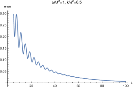
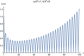
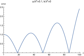
Figure 10: The relative difference between $G_{L}$ and the quenched result as a function of $L$ for different frequencies and momenta. Left: for a point in the $(\omega,k)$ plane which is outside of the shaded region of Fig. 9 the “error” goes to zero for large $L$. Middle: inside the shaded region the error is oscillating with diverging amplitude as $L$ goes to larger values. However, for larger values of $\omega$ there is an intermediate range of $L$, where the relative error is smaller than 0.3. Therefore the quenched approximation is qualitatively correct. Right: for small $\omega$ the amplitude of the oscillation is large.

References

- (1) J. Polchinski, “Effective field theory and the Fermi surface,” In *Boulder 1992, Proceedings, Recent directions in particle theory* 235-274, and Calif. Univ. Santa Barbara - NSF-ITP-92-132 (92,rec.Nov.) 39 p. (220633) Texas Univ. Austin - UTTG-92-20 (92,rec.Nov.) 39 p [hep-th/9210046]. arXiv:hep-th/9210046 [hep-th]
- (2) R. Shankar, “Renormalization group approach to interacting fermions,” Rev. Mod. Phys. 66, 129 (1994). arXiv:cond-mat/9307009 [cond-mat]
- (3) J. A. Hertz, “Quantum critical phenomena,” Phys. Rev. B 14 (1976) 1165
- (4) A. J. Millis, “Effect of a nonzero temperature on quantum critical points in itinerant fermion systems”, Phys. Rev. B48 (1993) 7183.
- (5) H. v. Löhneysen, A. Rosch, M. Vojta, P. Wölfle, “Fermi-liquid instabilities at magnetic quantum phase transitions,” Rev. Mod. Phys. 79, 1015 (2007). arXiv:cond-mat/0606317 [cond-mat]
- (6) S. Sachdev, “Quantum phase transitions,” Second edition, Cambridge University Press, 2011.
- (7) P. A. Lee, “Gauge field, Aharonov-Bohm flux, and high- superconductivity”, Phys. Rev. Lett. 63 (1989) 680.
- (8) V. Oganesyan, S. A. Kivelson, E. Fradkin, “Quantum theory of a nematic Fermi fluid”, Phys. Rev. B 64, 195109 (2001). arXiv:cond-mat/0102093 [cond-mat]
- (9) W. Metzner, D. Rohe, S. Andergassen, “Soft Fermi surfaces and breakdown of Fermi-liquid behavior”, Phys. Rev. Lett. 91, 066402 (2003). arXiv:cond-mat/0303154 [cond-mat]
- (10) M. A. Metlitski and S. Sachdev, “Quantum phase transitions of metals in two spatial dimensions: I. Ising-nematic order,” Phys. Rev. B 82 (2010) 075127 arXiv:1001.1153 [cond-mat.str-el]
- (11) M. A. Metlitski and S. Sachdev, “Quantum phase transitions of metals in two spatial dimensions: II. Spin density wave order,” Phys. Rev. B 82 (2010) 075128 arXiv:1005.1288 [cond-mat.str-el]
- (12) D. V. Khveshchenko and P. C. E. Stamp, “Low-energy properties of two-dimensional fermions with long-range current-current interactions”, Phys. Rev. Lett. 71 (1993) 2118
- (13) A. L. Fitzpatrick, S. Kachru, J. Kaplan and S. Raghu, “Non-Fermi liquid fixed point in a Wilsonian theory of quantum critical metals,” Phys. Rev. B 88 (2013) 125116 arXiv:1307.0004 [cond-mat.str-el]
- (14) A. L. Fitzpatrick, S. Kachru, J. Kaplan and S. Raghu, “Non-Fermi-liquid behavior of large- quantum critical metals,” Phys. Rev. B 89 (2014), 165114 arXiv:1312.3321 [cond-mat.str-el]
- (15) A. Allais and S. Sachdev, “Spectral function of a localized fermion coupled to the Wilson-Fisher conformal field theory,” Phys. Rev. B 90 (2014), 035131 arXiv:1406.3022 [cond-mat.str-el]
- (16) T. Holder, W. Metzner Fermion loops and improved power-counting in two-dimensional critical metals with singular forward scattering Phys. Rev. B92, 245128 (2015). arXiv:1509.07783 [cond-mat.str-el]
- (17) R. Mahajan, D. M. Ramirez, S. Kachru and S. Raghu, “Quantum critical metals in dimensions,” Phys. Rev. B 88 (2013), 115116 arXiv:1303.1587 [cond-mat.str-el]
- (18) J. Rech, C. Pepin, A. V. Chubukov, “Quantum critical behavior in itinerant electron systems: Eliashberg theory and instability of a ferromagnetic quantum critical point,” Phys. Rev. B, 74 195126 (2006), arXiv:cond-mat/0605306
- (19) A. L. Fitzpatrick, G. Torroba and H. Wang, “Aspects of Renormalization in Finite Density Field Theory,” Phys. Rev. B 91, 195135 (2015) arXiv:1410.6811 [cond-mat.str-el].
- (20) G. Torroba and H. Wang, “Quantum critical metals in dimensions,” Phys. Rev. B 90 (2014), 165144 arXiv:1406.3029 [cond-mat.str-el]
- (21) B. Meszena, P. Säterskog, A. Bagrov and K. Schalm, “Non-perturbative emergence of non-Fermi liquid behaviour in quantum critical metals,” Phys. Rev. B 94, 115134, arXiv:1602.05360 [cond-mat.str-el].
- (22) L. B. Ioffe, D. Lidsky, B. L. Altshuler, Effective lowering of the dimensionality in strongly correlated two dimensional electron gas, Phys Rev. Lett. 73 472 arXiv:cond-mat/9403023.
- (23) B. L. Altshuler, L. B. Ioffe, A. J. Millis, On the low energy properies of fermions with singular interactions, Phys. Rev. B50, 14048. arXiv:cond-mat/9406024.
- (24) W. Metzner, C. Castellani, C. Di Castro, Fermi Systems with Strong Forward Scattering, Adv. in Physics 47 317 (1998). [arXiv:cond-mat/9701012]
- (25) Tigran A. Sedrakyan and Andrey V. Chubukov, “Fermionic propagators for two-dimensional systems with singular interactions”, Phys. Rev. B, 79 (2009) 115129; arXiv:0901.1459
- (26) S. Raghu, G. Torroba, and H. Wang, “Metallic quantum critical points with finite BCS couplings,” Phys. Rev. B 92, (2015) 205104
- (27) P. Gegenwart, Q. Si, F. Steglich, “Quantum criticality in heavy-fermion metals,” Nature Physics 4, 186 - 197 (2008); arXiv:0712.2045 [cond-mat.str-el]
- (28) M. A. Metlitski, D. F. Mross, S. Sachdev and T. Senthil, “Cooper pairing in non-Fermi liquids,” Phys. Rev. B 91 (2015), 115111 arXiv:1403.3694 [cond-mat.str-el]
- (29) A. L. Fitzpatrick, S. Kachru, J. Kaplan, S. Raghu, G. Torroba and H. Wang, “Enhanced Pairing of Quantum Critical Metals Near d=3+1,” Phys. Rev. B 92 (2015), 045118 arXiv:1410.6814 [cond-mat.str-el]
- (30) H. Wang, S. Raghu, G. Torroba, “Non-Fermi liquid Superconductivity: Eliashberg versus the Renormalization Group,” Phys. Rev. B, 95 (2017), 165137, arXiv:1612.01971 [cond-mat.str-el]
- (31) A. Neumayr and W. Metzner, “Fermion loops, loop cancellation and density correlations in two-dimensional Fermi systems,” Phys. Rev. B 58 (1998) 15449 arXiv:cond-mat/9805207 [cond-mat]
- (32) S. C. Thier and W. Metzner, “Singular order parameter interaction at the nematic quantum critical point in two-dimensional electron systems”, Phys. Rev. B 84 (2011) 155133, arXiv:1108.1929 [cond-mat.str-el]
- (33) P. Kopietz, J. Hermisson, and K. Sch nhammer, “Bosonization of interacting fermions in arbitrary dimension beyond the Gaussian approximation,” Phys. Rev. B 52 (1995) 10877 arXiv:cond-mat/9502089 [cond-mat]
- (34) T. Granlund et al.,“GNU Multiple Precision Arithmetic Library”, gmplib.org
- (35) S. S. Lee, “Low-energy effective theory of Fermi surface coupled with U(1) gauge field in 2+1 dimensions,” Phys. Rev. B 80 (2009) 165102; arXiv:0905.4532 [cond-mat.str-el]
- (36) D. F. Mross, J. McGreevy, H. Liu and T. Senthil, “A controlled expansion for certain non-Fermi liquid metals,” Phys. Rev. B 82 (2010) 045121; arXiv:1003.0894 [cond-mat.str-el]
- (37) Y. B. Kim, A. Furusaki, X. G. Wen and P. A. Lee, “Gauge-invariant response function of fermions coupled to a gauge field”, Phys. Rev. B 50 (1994) 17917, arXiv:cond-mat/9405083 [cond-mat]