Towards the Formalization of a Factory Demonstrator in BeSpaceD

Abstract

This report gives an overview of our efforts towards a formalization for a food processing demonstrator plant. Our BeSpaceD framework is used for the formalization. The formalization comprises properties of components and relations between components. We present domain-specific constructs for the formalization of industrial automation facilities and provide some insights into the concrete food processing formalization. We are particularly interested in spatio-temporal and other physical characteristics. Relationships are formalized as graphs with annotated edges and components are represented as nodes.

1 Introduction

This report continues a series of documents [2, 4, 12] around our spatio-temporal modelling and reasoning framework BeSpaceD[1]. In this report we use the BeSpaceD language in a domain specific modelling task, namely a factory demonstrator for food processing. The models cover a variety of spatial and temporal aspects of the factory including physical location and sizing, meta-data about each component, temporal correlations between actuators and sensors as well as temporal safety margins between actuating.

BeSpaceD is our framework for spatio-temporal modelling and reasoning[8, 7]. BeSpaceD is implemented using Scala and provides (i) spatio-temporal constructs for defining components and their relationship especially with respect to time and space, and (ii) other basic logic constructs to specify properties and models. BeSpaceD is open source and the work described in this report is part of the main development repository. The formalization presented here primarily serves academic purposes and is a candidate for a reference formalization and example for future efforts.

In addition to industrial automation [5, 6], BeSpaceD has been applied to mobile systems [16, 15] using the reactive blocks tool set [17], the verification of wireless network setups [13] and in the area of smart energy systems [3, 18]. The work described in this paper makes use of qualitative spatial representations [11, 10] following ideas similar to principles of the region connection calculus [19]. Initial ideas for the formalization of the demonstrator that is subject to this report have been discussed in [14]. The factory demonstrator is also part of our VxLab activities [9].

Overview

We provide a short overview on BeSpaceD in Section 2. Domain specific constructs for industrial automation are provided in Section 3 and Section 4 introduces our demonstrator. Section 5 provides the formalization of the example system using BeSpaceD. A conclusion is featured in Section 6.

2 BeSpaceD

The modelling constructs we use for the industrial automation domain are built on some generic data structures in the BeSpaceD core language. BeSpaceD provides some primitives for representing symbolic scalars and integers, component meta-data, events, time and space. BeSpaceD builds most of its constructs on two foundational types:

    trait Invariant extends Ordered[Invariant]
    trait ATOM extends Invariant

An Invariant is a formula that is supposed to hold for a system. An ATOM is a special case of Invariant that is not composed of multiple invariants. Time and space are of primary concern in BeSpaceD. BeSpaceD represents time with the following constructs:

    case class TimePoint [+T] (timepoint : T) extends ATOM
    case class TimeInterval[+T](timepoint1 : T, timepoint2 : T) extends ATOM

BeSpaceD represents geometric space with many occupational constructs. Here, we primarily use:

    case class Occupy3DBox (x1 : Int, y1: Int, z1 : Int,
                            x2 : Int, y2 : Int, z2 : Int)
         extends ATOM

BeSpaceD represents events with a single construct called Event:

    case class Event [+E] (override val event  : E) extends ATOM

For our modelling effort in industrial automation we extend the the BeSpaceD language in a number of areas. The rest of this section presents these extensions.

2.1 Controller Events

BeSpaceD represents events with a single construct called Event, and a generalization called EventLike:

    trait EventLike  [+E] extends ATOM { val event: E }
    case class Event [+E] (override val event  : E) extends EventLike[E]

In the industrial automation domain an event is something that changes state at an instant in time. There is a construct in BeSpaceD to reflect these semantics:

    class INSTATE[+O, +T, +S] (val owner : O, val timepoint : TimePoint[T],
                               val state :S)
          extends Event[(O,TimePoint[T],S)]( (owner, timepoint, state) )

The value passed to the superclass Event’s constructor is a tuple of cardinality three which maintains compatibility with the more general Event.

2.2 Structural Extensions

We define meta-data for each of the components that make up a machine. This data lends itself to a key-value style encoding. In order to support this style we added the following BeSpaceD structural constructs to tag data with semantics in the context of this key-value encoding style:

    case class Component[+I] (id : I) extends ATOM
    case class ComponentValue[+V] (value : V) extends ATOM

Component defines the keys and ComponentValue defines the values. By convention, the keys identify a single component. The type could be a string or a reference to any domain specific component. In our case the component ID’s are stings used to define a unique name for each.

Meta data is defined in BeSpaceD as a conjunction (BIGAND) of key value pairs, where each pair is an implication (IMPLIES). This is very similar to a ”Map” in mathematics and many programming languages. BeSpaceD provides the BeMap construct (a specialization of BIGAND) which extends the relatively simple BIGAND with map like behaviour:

    class BeMap[+P <: Invariant, +C <: Invariant](terms: List[IMPLIES[P,C]])
        extends BIGAND[IMPLIES[P,C]](terms)
        {
          lazy val premises    = ( this.terms map { _.premise } ).toSet[Any]
          lazy val conclusions = ( this.terms map { _.conclusion } ).toSet[Any]
          lazy val elements    = premises union conclusions

          def apply(key: Invariant): Option[C]
        }

BeMaps are used to construct the descriptions using Component as the key and ComponentValue as the value:

    case class ComponentDescription[+C <: Component[Any],
                                    +V <: ComponentValue[Any]]
               (override val terms: List[IMPLIES[C,V]])
         extends BeMap[C,V](terms)

An example construction of meta data is shown below:

    val elon = BeMap(
        Component("Name")    ==> ComponentValue("Elon Musk"),
        Component("Address") ==> ComponentValue("Mars")
        )

An example query of a BeMap can be done as follows:

    elon("Address")

2.3 Topological Extensions

To support the use of graphs for defining topologies we added a graph construct to BeSpaceD. In our model the edges are annotated so the existing BeSpaceD Edge primitive is extended to support annotations of any type:

    class EdgeAnnotated[+N, +A] (val source : N, val target : N,
                                 val annotation: Option[A])
          extends ATOM
    case class Edge[+N] (override val source : N, override val target : N)
         extends EdgeAnnotated[N,{\tt Nothing}](source, target, None)

It is interesting to note, in type inheritance terms, Edge is a specialisation of EdgeAnnotated. On the surface, this may feel counter-intuitive, however, it makes sense when you consider that Edge proper is a special kind of edge annotated with nothing. Scala provides a special type called Nothing that is a specialisation of all other types and we make use of this feature.

The Edge and EdgeAnnotated constructs define edges with two nodes. We define graphs as a BIGAND of annotated edge objects called BeGraphAnnotated. The non-annotated version is called a ”BeGraph” for behavioural graph.

    class BeGraphAnnotated[+N, +A](terms: List[EdgeAnnotated[N, A]])
          extends BIGAND[EdgeAnnotated[N, A]](terms)Ψ
    class BeGraph[+N](terms: List[Edge[N]])
          extends BeGraphAnnotated[N, Nothing](terms)

An example construction of a simple graph would be:

    BeGraph(
           Component("Smoke Detector") --> Component("Alarm"),
           Component("Motion Sensor") --> Component("Alarm")
           )

The --> symbol is a binary infix operator that constructs an Edge object.

2.4 Temporal Extensions

We model a number of different topologies for the industrial automation domain most of which require temporal semantics. We extended BeSpaceD with two temporal constructs to represent timing relationships: correlations and constraints. A temporal correlation declares that two events coincide with a specified time delay relative to the first event. The first event is called the ”cause” and the second, ”effect”.

    case class TemporalCorrelation[+E, +T <: Number]
         (cause: EventLike[E], duration: TimeDuration[E], effect: EventLike[E])
         extends Invariant

A temporal constraint declares that two events (or one event and the lack of a second event in the inverse case) occur within a specified time duration relative to the first event.

case class TemporalConstraint [+E, +T <: Number]
           (cause: EventLike[E], range: TimeDurationRange[E],
            effect: EventLike[E], inverse: Boolean = false)
     extends Invariant

3 Domain Specific Modelling for Industrial Automation

We identified many data structures that are reusable within the industrial automation domain which are kept separated from applications. For the modelling exercise we considered programmable logic controllers (PLC) outside the scope. The industrial automation domain meta-model is defined in the BeSpaceDIA project and defines types which, in effect, present design patterns for developers of more specific domains such as food processing. In this section we categorize and summarize all the domain specific types in the PhysicalModel module of BeSpaceDIA.

3.1 Object Identity

We provide a trait for each kind of physical object and then break this down into a generalised type hierarchy representing components of automation equipment.

    trait PhysicalObject[+I]       extends Component[I]

A device represents any built in component of the machine itself. This is further broken down into parts, actuators and sensors. A Part represents a device that forms part of a useful process. An actuator is a device that connects PLCs with parts to make them do something. A sensor is a device that communicates some portion of the state of the machine back to the PLC.

    trait Device[+I]               extends PhysicalObject[I]
    trait Part[+I]                 extends Device[I]
    trait Actuator[+I]             extends Device[I]
    trait Sensor[+I]               extends Device[I]

Material represents physical things that pass through the machine but are not considered part of the machine itself. A discrete material represents atomic objects that should not be divided; for example bottle caps. There is no point it measuring fractions of a cap, so these can be measured using natural numbers. An analog material represents a divisible material where we can measure it using a real number; for example, water.

    trait Material[+I]             extends PhysicalObject[I]
    trait DiscreteMaterial[+I]     extends Material[I]
    trait AnalogMaterial[+I]       extends Material[I]
          { val unit: String; val quantity: Double }

All physical objects have an identity. With regards to discrete materials there is the ability to uniquely identify each one, for example each bottle cap can have a unique identity. This would allow one to trace discrete materials through the system.

3.2 Spatial Variation

The following type is defined for creating an application specific spatial variation:

    trait SpatialVariation extends Invariant

This allows the applications to model a set of discrete values representing positions in space (like an enumerated type). This is done in Scala using singleton objects which extend the SpatialVariation trait, for example:

    abstract class StackEjectorPosition extends ATOM with SpatialVariation
    object StackEjectorRetractedPosition extends StackEjectorPosition
    object StackEjectorExtendedPosition extends StackEjectorPosition

3.3 State Types

The following types are defined for creating application specific states:

    trait PhysicalState[+S]           extends ComponentState[S]
    trait DeviceState[+DS]            extends PhysicalState[DS]
    trait PartState[+PS]              extends DeviceState[PS]
    trait ActuatorState[+AS]          extends DeviceState[AS]
    trait SensorState[+SS]            extends DeviceState[SS]

This allows the applications to model a set of discrete values representing all the useful abstract states for each category of device, for example:

    abstract class LightSensorState(sig: Signal) extends SensorState(sig)
    class ObstructedState(sig: Signal) extends LightSensorState(sig)
    val ObstructedHigh   = ObstructedState(High)
    val ObstructedLow    = ObstructedState(Low)
    val Obstructed       = ObstructedState(DC)

Obstructed is an abstract state and ObstructedHigh additionally records the actual domain specific electrical signal that indicates this state.

3.4 Events

The following types are defined for creating application specific events:

    abstract class PhysicalEvent[+I, S](component: PhysicalObject[I],
                                        timepoint: TimePoint[Long],
                                        state: PhysicalState[S])
             extends INSTATE[PhysicalObject[I], Long, PhysicalState[S]]
                     (component, timepoint, state)
             with BeSpaceDGestalt.core.Event[S]

    abstract class DeviceEvent[+I, S](device: Device[I],
                                      timepoint: TimePoint[Long],
                                      state: DeviceState[S])
             extends PhysicalEvent[I, S](device, timepoint, state)

    abstract class ActuatorEvent[+I, S](actuator: Actuator[I],
                                        timepoint: TimePoint[Long],
                                        state: ActuatorState[S])
             extends DeviceEvent[I, S](actuator, timepoint, state)

    abstract class SensorEvent[+I, S](sensor: Sensor[I],
                                        timepoint: TimePoint[Long],
                                        state: SensorState[S])
             extends DeviceEvent[I, S](sensor, timepoint, state)

The following allows the application to model live events describing changes in the state of the factory, for example:

    SensorEvent(StackEmpty, TimePoint(new Date()), Obstructed)

This means the relevant light sensor has detected the stack is empty.

3.5 Topologies

The following types are defined for creating application specific topologies:

    abstract trait Relationship
    abstract trait SpatialRelationship extends Relationship
    abstract trait TemporalRelationship extends Relationship
    abstract trait SpatioTemporalRelationship
             extends SpatialRelationship with TemporalRelationship

    type Topology[+COM <: Component[Any], +REL <: Relationship] =
         BeGraphAnnotated[COM, REL]
    type SpatialTopology[+COM <: Component[Any],
                         +SREL <: SpatialRelationship] =
         BeGraphAnnotated[COM, SREL]
    type TemporalTopology[+COM <: Component[Any],
                          +TREL <: TemporalRelationship] =
         BeGraphAnnotated[COM, TREL]
    type SpatioTemporalTopology[+COM <: Component[Any],
                                +STREL <: SpatioTemporalRelationship] =
         BeGraphAnnotated[COM, STREL]

The following allows the applications to model functional, spatial and/or temporal relationships between devices, for example:

        case class Seconds(s: Int)
             extends TimeDuration(s) with SpatialRelationship

        BeGraphAnnotated (
            EdgeAnnotated(Component("Smoke Detected"),
                          Component("Alarm Activated"),
                          Some(Seconds(1))),
            EdgeAnnotated(Component("Smoke Clear"),
                          Component("Alarm Deactivated"),
                          Some(Seconds(3)))
            )

4 The Example Factory Demonstrator

The food processing factory used in our demonstrator is scaled down version of a fully functioning factory system capable of filling bottles with liquid or corn kernels, capping the bottles, moving bottles on conveyer belts and supplying both bottles and caps from storage.

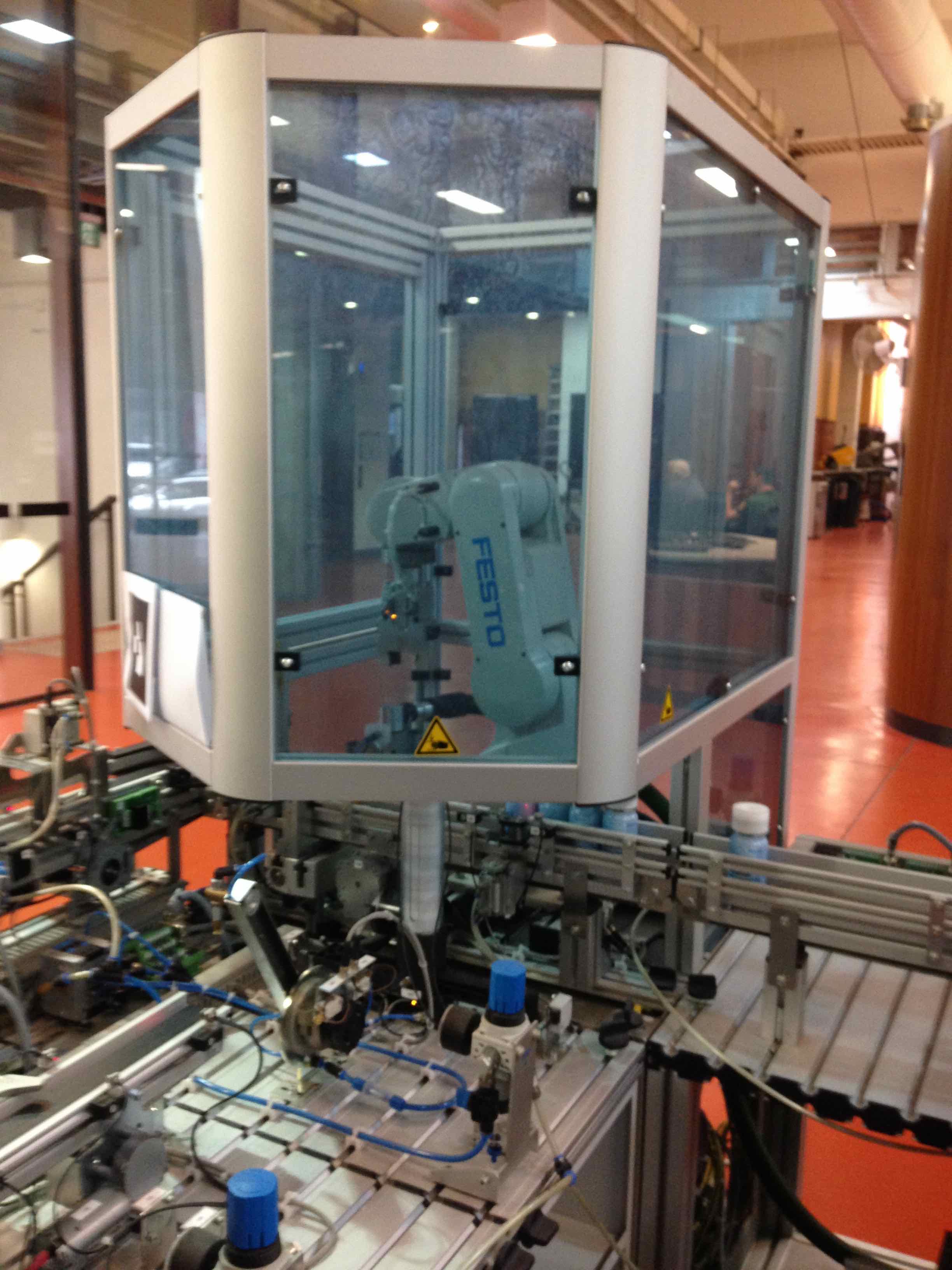
Figure 1: Station one

4.1 Scope

For this modelling application we limit the scope to a single station (as seen in Figure 1) which is controlled by a single PLC. The originally provided PLC is replaced with a customized Raspberry Pi based PLC solution which allows us to run BeSpaceD and communicate to both the station and the cloud over a wifi network. We numbered this Station one and named it “CapDispenser”. Other stations that are out of scope but we have partially modelled include: CapConveyer, Capping, RotaryTablePart1, RotaryTablePart2, CappedBottlesConveyerBelt, PackagingStation, BottleConveyer and BottleConveyerSorting.

The CapDispenser Station involves two subsystems (as seen in Figure 2).

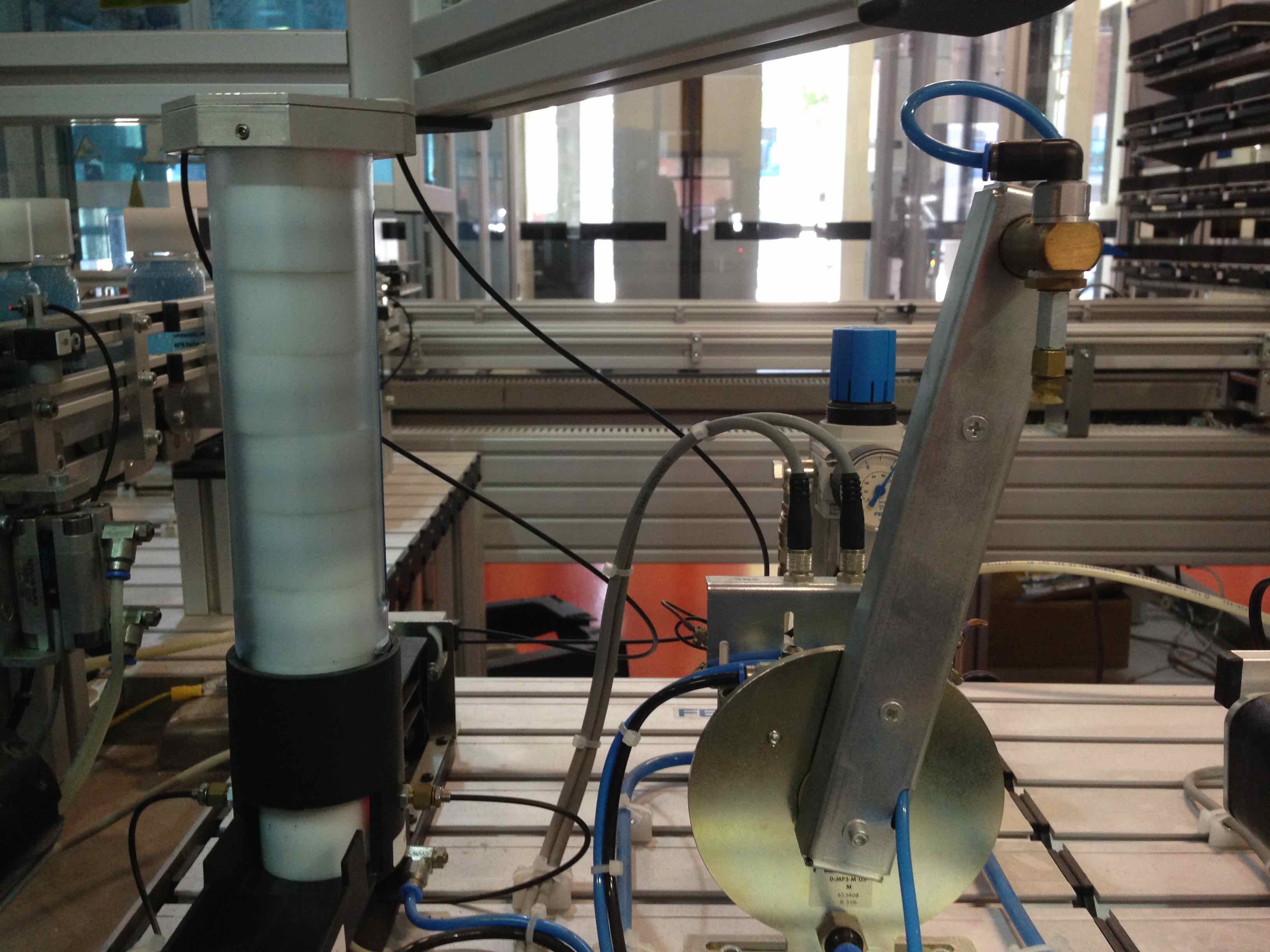
Figure 2: Two subsystems of station one

• A tube to hold caps with a cap ejector underneath that pushes caps out of the tube (see Figure 3).

  

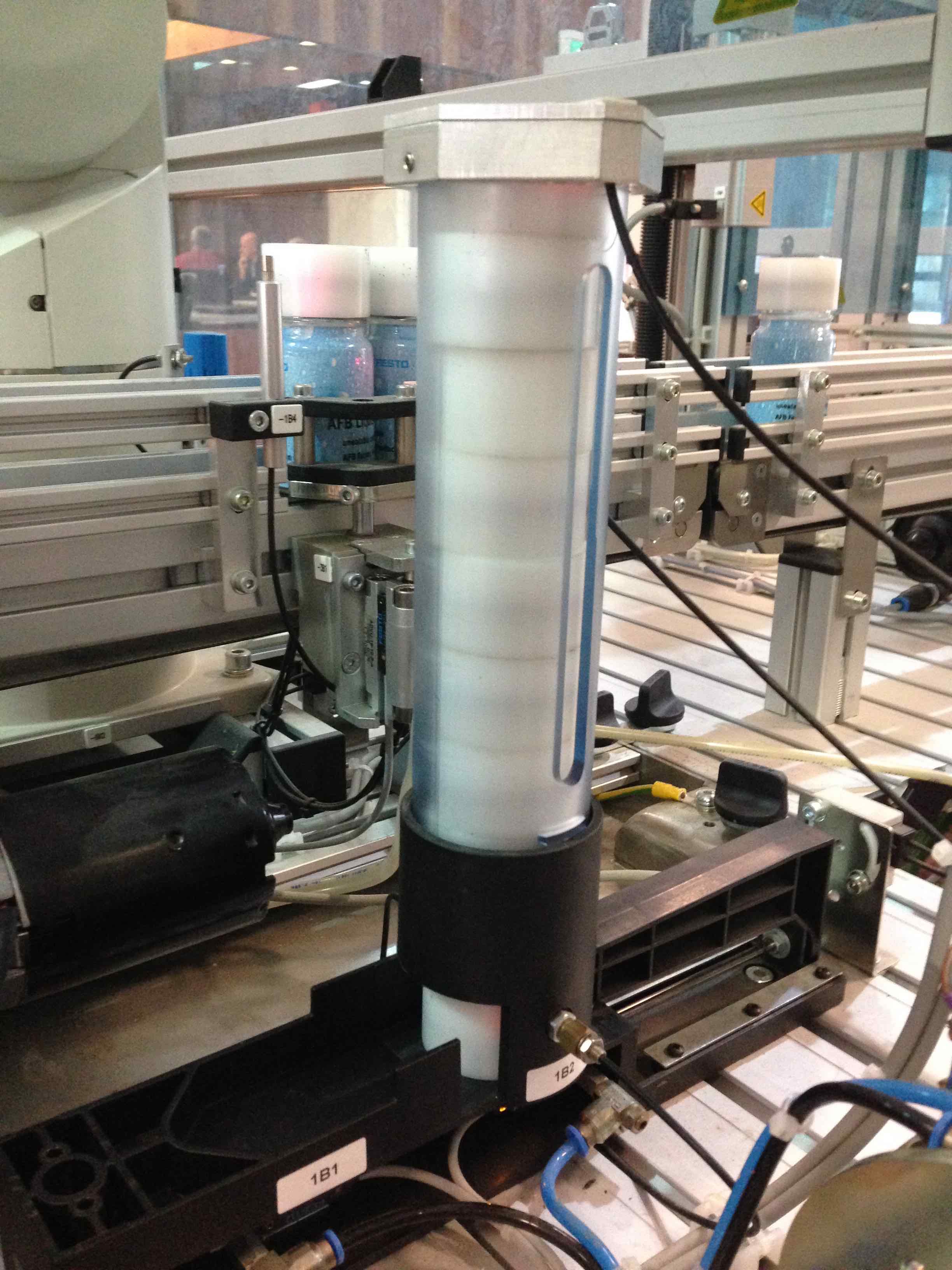
  Figure 3: Cap stack and ejector

• A lever arm (that swings in an arc) with a vacuum gripper built into the tip of the arm used to pick up and drop off caps (see Figure 4).

  

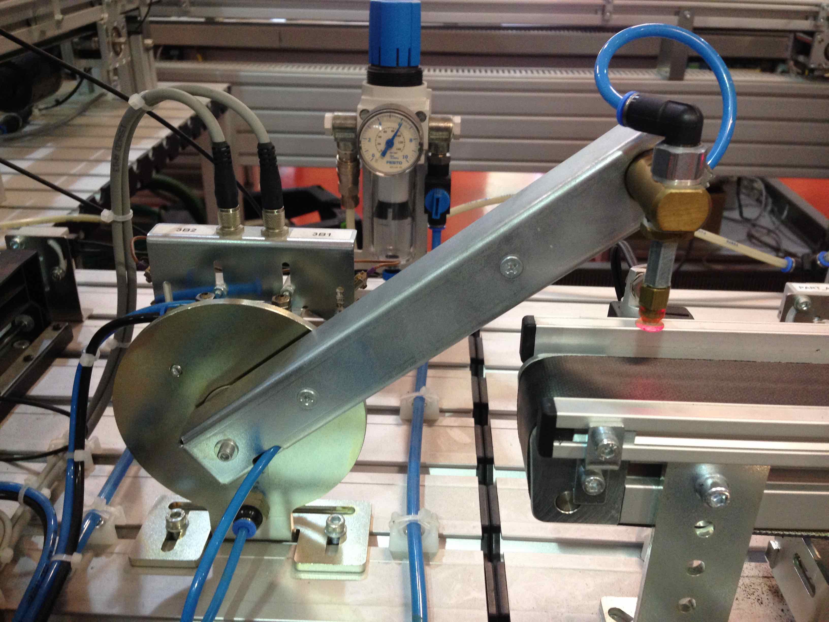
  Figure 4: Lever arm with vacuum gripper

4.2 Description of the Cap Dispenser Station

In this section we describe the two subsystems of the Cap Dispenser station in more detail including the parts, actuators and sensors.

4.2.1 The Cap Stack and Ejector

There is only one actuator integrated into the cap ejector part:

• Stack Ejector Extend: Activation causes the ejector to be extended which pushes out the bottom cap in the stack if there is one.

• Stack Ejector Extend: Inactivation causes the ejector to be retracted which returns the ejector to the original position and causes the rest of the caps to move down one cap height in the stack due to gravity.

There are three sensors integrated into the cap tube and ejector parts:

• Stack Empty: A light sensor positioned at the base of the tube that when unobstructed indicates the tube is empty.

• Stack Ejector Extended: A light sensor positioned at the extreme extended position of the ejector. When obstructed this indicates the stack ejector has been fully extended.

• Stack Ejector Retracted: A light sensor positioned at the extreme retracted position of the ejector. When obstructed this indicates the stack ejector has been fully retracted.

4.2.2 Pick-and-Place Unit

There are four actuators integrated into the cap loader and vacuum gripper parts:

• Loader Pickup: Activation causes the arm to rotate to the left towards the pickup area.

• Loader Dropoff: Activation causes the arm to rotate to the right towards the drop-off area.

• Vacuum Grip: Activation causes the vacuum motor to pump air out of the suction cup mounted in the tip of the lever arm.

• Eject Air Pulse: Activation causes the pulse motor to pump air into the suction cup causing the cup to loose suction.

There are three sensors integrated into the cap loader and vacuum gripper parts:

• Loader Picked Up: A contact sensor that indicates the arm has fully rotated into the pickup area.

• Loader Dropped Off: A contact sensor that indicates the arm has fully rotated into the drop-off area.

• Workpiece Gripped: A sensor that indicates the vacuum has reached a level where suction force is greater than the gravitational force of a bottle cap (i.e. it is gripped and should not fall off).

5 Demonstrator Formalization

We divide our model of the food processing factory domain into four distinct areas:

• Components - For modelling the identity of each physical component in the factory. For this domain we call the components “Devices”.

• Meta data - For modelling static data about the components. For this domain we call this data “Device Descriptions”. Spatial data is included in the descriptions.

• Topologies - For modelling information in a graph structure. For this domain we experimented with a few topologies representing different information.

• Events - For modelling Dynamic data (i.e. data that is defined in time).

Each area is described in more detail below including definitions of the data structures used and some example code snippets.

5.1 Devices (Components)

The model of devices provides a uniform way to identify every component in the factory. As per the industrial automation domain model we define three categories of devices: parts, actuators and sensors. We ensure the BeSpaceD Component construct is used to define every device by reusing the Device class defined for the industrial automation domain.

    trait FestoDevice extends Device[ID]

We define the identity type for all devices as a String and use a type alias called ID.

    type ID = String

This type is used consistently throughout the model where identity is required. Finally, we define the three sub devices for this domain:

    class FestoPart(override val id: ID)
          extends Component(id) with Part[ID] with FestoDevice
    class FestoActuator(override val id: String)
          extends Component(id) with Actuator[ID] with FestoDevice
    class FestoSensor(override val id: ID)
          extends Component(id) with Sensor[ID] with FestoDevice

5.2 Device Descriptions

To construct device descriptions realizing meta data in the domain model we re-use the BeSpaceD ComponentDescription class and refine the constructor parameter to be a behavioral map:

    class FestoComponentDescription(entries: BeMap[Component[Any],
                                                   ComponentValue[Any]])
          extends ComponentDescription[Component[Any],ComponentValue[Any]]
                  (entries.terms)

Each device category requires different meta-data. First we introduce a few concepts in Section 5.2.1. Then we define the data common to all devices in Section 5.2.2 followed by the meta data specific to each device category in its own section.

5.2.1 Anatomy of a Part Description

To illustrate the structure of the device descriptions we will briefly delve deep into one simple example; the StackEjector part. (the "==>" symbol is a binary infix operator for the BeSpaceD IMPLIES construct). Here is how we define it at the top level:

    val exampleEntry =  Component(StackEjector)  ==>
                        FestoComponentDescription(isPart, isHorizontalPusher,
                        stackEjectorVariations, stackEjectorOccupy)

And this is what the parameters mean and how we construct them: The device category and type is meta data about the type of the device and are simply key-value pairs constructed using an IMPLIES construct.

    val isPart               = DeviceCategory ==> Part
    val isHorizontalPusher   = DeviceType     ==> HorizontalPusherPart

Spatial variations represent a discrete set of spatial positions that a part can be “in”. First, we define the set of demonstrator specific positions, and then map this to a mutual exclusion structure of component values. We use the BeSpaceD exclusive or XOR logical construct to represent mutual exclusion.

    val StackEjectorPositions = XOR(StackEjectorRetractedPosition,
                                    StackEjectorExtendedPosition
                                    )
    val stackEjectorVariations = SpatialVariations ==>
                                     ComponentValue(XOR(
                                         StackEjectorPositions.terms map
                                             {pos => ComponentValue.apply(pos)}
                                         )
                                     )

Figure 5 represents the above spatial variations as a graph of BeSpaceD objects.

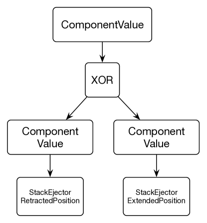
Figure 5: Spatial variations as a BeSpaceD object graph

The last parameter, stackEjectorOccupy, defines the three dimensional space which the part occupies:

    val stackEjectorOccupy = SpatialLocation ==>
          ComponentValue(Occupy3DBox(
             X.StackEjectorLeft, Y.StackEjectorFront, Z.StackEjectorBottom,
             Width.StackEjector, Depth.StackEjector, Height.StackEjector
          ))

The parameters in the Occupy3DBox above are constant measurements. How we define these measurements is discussed further in subsection 5.2.7.

5.2.2 Overview of all Device Descriptions

The meta data for multiple devices includes the keys: DeviceCategory, DeviceType, GPIO, PartAssociation, SignalMapping and SpatialLocation. Well known values are defined for the first three keys; for example:

    // Device Categories
    val Part           = ComponentValue("Part")
    val Actuator       = ComponentValue("Actuator")
    val Sensor         = ComponentValue("Sensor")

    // Device Types
    val SolenoidActuator = ComponentValue("Solenoid")
    val LightSensor = ComponentValue("Light Sensor")

    // GPIO Pins - Actuators
    val GPIO_1  = ComponentValue(1)
    val GPIO_26 = ComponentValue(26)

    // GPIO Pins - Sensors
    val GPIO_7  = ComponentValue(7)
    val GPIO_25 = ComponentValue(25)

The GPIO Pins are either used for a sensor or an actuator, not both.

5.2.3 Signal Mapping

Our factory demonstrator comes with a variety of actuators and sensors. In station one, they all have binary signalling which means there are only two voltage levels generated or accepted. These signals are named High (for a high voltage level) and Low (for a low voltage level). It would be perfect if every actuator interpreted High as activation and every light sensor generated a High signal for an obstructed state. Unfortunately, this semantic mapping is inconsistent between devices, even in station one of our demonstrator factory. Some solenoid based actuators activate on High and some on Low. Some light sensors when obstructed generate High and others Low. So we need a functional mapping between signal level and its meaning.

We encode the meaning of the signal to/from each actuator/sensor in a signal mapping data structure. To model the meaning, we use the State types defined in the industrial automation domain model (see Section 3.3). The embedded object is of any type and allows us to create domain specific types for the demonstrator domain. In our case we created the following signal types:

    class FestoSignal(val state: String)
    case object High extends FestoSignal("High")
    case object Low  extends FestoSignal("Low" )
    case object DC   extends FestoSignal("Don’t Care" )

And them embed in the device states:

    class FestoActuatorState(signal: FestoSignal)
          extends FestoDeviceState(signal) with ActuatorState[FestoSignal]
    class FestoSensorState(signal: FestoSignal)
          extends FestoDeviceState(signal) with SensorState[FestoSignal]

The DC signal is used to specify an abstracted device state where we don’t care what the voltage signal actually is or will be. In the application domain specific model, constants are defined for all the device states, for example actuators that use a solenoid are defined as follows:

    abstract class FestoSolenoidActuatorState(signal: FestoSignal)
             extends FestoActuatorState(signal)
    class ActiveState(sig: FestoSignal)
          extends FestoSolenoidActuatorState(sig)
    class PassiveState(sig: FestoSignal)
          extends FestoSolenoidActuatorState(sig)

    val ActiveHigh  = ActiveState(High)
    val ActiveLow   = ActiveState(Low)
    val Active      = ActiveState(DC)
    val PassiveHigh = PassiveState(High)
    val PassiveLow  = PassiveState(Low)
    val Passive     = PassiveState(DC)

Objects of these types are used in the mapping to describe the meaning of the signal. The signal mapping function is defined as: :

    type SignalTo[R]           = Map[FestoSignal, R]
    type SignalSensorMapping   = SignalTo[FestoSensorState]
    type SignalActuatorMapping = SignalTo[FestoActuatorState]

and used for example in the following way:

    val HighSolenoidActuatorMapping: SignalActuatorMapping =
            Map(High -> ActiveHigh,  Low -> PassiveLow)

    val SignalMapping = Component("Signal Mapping")
    val isHighSolenoidActuator =
            SignalMapping ==> ComponentValue(HighSolenoidActuatorMapping)

5.2.4 Parts

The meta data for parts includes the key SpatialVariations and an example of a well known value is:

    val ConveyerPart         = ComponentValue("Conveyer")
    val isConveyer           = DeviceType ==> ConveyerPart

A spatial variation defines a discrete set of positions for a moving part semantically as discussed in Section 5.2.1.

5.2.5 Actuators

Actuators are defined in terms of the common keys, however, they do have some specific well known values such as:

    val SolonoidActuator = ComponentValue("Solonoid")
    val isSolonoid = DeviceType ==> SolonoidActuator

An example description for the vacuum gripper actuator is:

    val forLoader = PartAssociation   ==> ComponentValue(Loader)
    Component(VacuumGrip) ==> FestoComponentDescription(
                              isActuator, isSolonoid, isGpio5,
                              isHighSolonoidActuator, forLoader)

Note, the spatial occupation data has been left out. A topic for future work would be how to model spatial occupation when it is not fixed relative to the machine but will be moving relative to how the part it is embedded in moves. The isHighSolonoidActuator is a signal mapping function (see Section 5.2.3) that declares that a high voltage activates the solenoid and a low voltage inactivates it.

5.2.6 Sensors

Sensors have some specific well known values such as:

    val LightSensor = ComponentValue("Light Sensor")
    val isLightSensor = DeviceType ==> LightSensor

An example of a sensor description follows. It uses the same meta data keys as the actuators:

    Component(StackEjectorExtended)  ==> FestoComponentDescription(
                                      isSensor, isLightSensor, isGpio0,
                                      isHighLightSensor, forStackEjector,
                                      stackEjectorExtendedOccupy)

The stackEjectorExtendedOccupy parameter is spatial data and is explained in the following Section 5.2.7.

5.2.7 Spatial Meta Data

We use the Occupy3DBox core construct to define the volume of space occupied by a device. The desired result of an Occupy3DBox is quite simple, however, the steps to construct one is not so simple. we did this in an elegant way that minimises the number of measurements that need to be taken by reusing the measurements of key reference points and sizes. Below is a partial extract of the measurement code and serves as an example for the two light sensors in the proximity of the cap ejector part:

    object X {
      val Station1EdgeLeft         = 0
      val StackEjectorRight        = Station1EdgeLeft + 85
      val ExtendRetractSensorRight = StackEjectorRight
      val ExtendRetractSensorLeft  = ExtendRetractSensorRight - Width.ExtendRetractSensor
    }
    object Y {
      val Station1EdgeFront        = 0
      val StackEjectorFront        = Station1EdgeFront + 76

      val ExtendSensorFront        = StackEjectorFront + 122
      val ExtendSensorBack         = ExtendSensorFront + Depth.ExtendRetractSensor

      val RetractSensorFront       = StackEjectorFront + 236
      val RetractSensorBack        = RetractSensorFront + Depth.ExtendRetractSensor
    }
    object Z {
      val Base                        = 0
      val StackEjectorBottom          = Base
      val ExtendRetractSensorBottom   = Base + 4
      val ExtendRetractSensorTop      = Base + 20
    }
    object Width {
      val ExtendRetractSensor = 32
    }
    object Depth {
      val ExtendRetractSensor = 10
    }
    object Height {
      val ExtendRetractSensor = Z.ExtendRetractSensorTop -
                                Z.ExtendRetractSensorBottom
    }

Note, that the width, depth and height metrics are reused for both sensors as are the x and z coordinates. The y coordinate is different for each sensor and so is separated. In addition, reference metrics are used that are reused to build up the actual metric symbolically. There are several layers of referencing including the base of the station one, the edge of a part and the edge of sensor or actuator. These layers are referenced by downstream layers to formulate the metrics. Finally some meta data can be created for defining the spatial occupation for the sensor’s descriptions:

    val stackEjectorExtendedOccupy  = occupy(
                                         X.ExtendRetractSensorLeft,
                                         Y.ExtendSensorFront,
                                         Z.ExtendRetractSensorBottom,
                                         Width.ExtendRetractSensor,
                                         Depth.ExtendRetractSensor,
                                         Height.ExtendRetractSensor)

    Component(StackEjectorExtended)  ==> FestoComponentDescription(
                                            isSensor, isLightSensor, isGpio0,
                                            isHighLightSensor, forStackEjector,
                                            stackEjectorExtendedOccupy)

    val stackEjectorRetractedOccupy = occupy(
                                         X.ExtendRetractSensorLeft,
                                         Y.RetractSensorFront,
                                         Z.ExtendRetractSensorBottom,
                                         Width.ExtendRetractSensor,
                                         Depth.ExtendRetractSensor,
                                         Height.ExtendRetractSensor)

    Component(StackEjectorRetracted) ==> FestoComponentDescription(
                                            isSensor, isLightSensor, isGpio3,
                                            isHighLightSensor, forStackEjector,
                                            stackEjectorRetractedOccupy)

Notice that the OccupyBox objects are consistently built from the left, front and bottom coordinates as well as the width, depth and height sizes for each sensor.

In this section we have seen step by step how spatial data for the volume occupied by a device is built from a few measurements with layered symbolic referencing.

5.3 Topologies

So far we have only addressed static meta data oriented around components. In this section we show how we modelled information in a topological structure. We have developed several different but complimentary topologies that illustrate the possibilities that BeSpaceD offers in modelling topological information and these are presented in the following.

5.3.1 Sensor Process Sequence

The first topology involves only sensors and captures the expected order of state change in a set of sensors as material flows through the machine during normal processing scenarios. The process flow topology is illustrated in Figure 6.

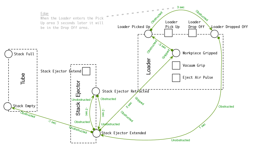
Figure 6: Process flow topology

Each edge in the topology represents a temporal proximity relationship: A state change in one sensor (source node) is expected to be soon followed by a state change in another sensor (destination node). The way we model this is by representing sensors as nodes and the expectation as edges. Each edge is annotated with three pieces of information:

• Cause: the state change of the first sensor. This is done by annotating the leading edge with the value the sensor state changes TO.

• Duration: the exact time between the two state changes.

• Effect: the state change of the second sensor. This is done by annotating the trailing edge with the value the sensor state changes TO.

The BeSpaceD encoding of the annotations use a TemporalCorrelation as follows:

    class  FestoStateCorrelation(
              cause: FestoDeviceState,
              duration: TimeDuration[FestoDeviceState],
              effect: FestoDeviceState)
    extends TemporalCorrelation[FestoDeviceState, Integer]
            (cause, duration, effect)

Below is an example of one such process sequence edge in BeSpaceD serialised to JSON (this edge is the same one commented on in Figure 6):

{
    "type" : "EdgeAnnotated",
    "source" : {"type":"Component","id":"Loader Picked Up"},
    "target" : {"type":"Component","id":"Loader Dropped Off"},
    "annotation" : {
        "type": "FestoStateCorrelation",
        "cause": {"type": "Obstructed"},
        "duration": {
            "type":"TimeDuration",
            "start":{"type": "SS Variable", "expression": {"type": "Obstructed"}},
            "scalar":{"type": "SS Addition", "expression": [
                     {"type": "SS Variable", "expression": {"type": "Obstructed"}},
                     {"type": "SS Constant", "expression": 3}
                     ]}
             },
         "effect": {"type": "Obstructed"}}
    }

Notice that this topology does not allow for any variability in the timing so it would be best suited for modelling real world data inferred from live events.

5.3.2 Actuator-Sensor Causality

The causality topology is illustrated in Figure 7.

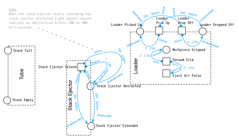
Figure 7: Causality topology

Each edge in the causality topology represents a temporal proximity relationship between an actuator to a sensor: A state change in an actuator (source node) leads to a state change in a sensor (destination node). We assert that this must happen within some time range. The way we model this is by representing devices as nodes and the assertion as edges. Each edge is annotated with three pieces of information:

• Cause: the state change of the actuator. This is done by annotating the leading edge with the value the actuator state changes TO.

• Duration Range: One minimum and one maximum time duration.

• Effect: the state change of the sensor. This is done by annotating the trailing edge with the value the sensor state changes TO.

The BeSpaceD encoding of these annotations use a TemporalConstraint as follows:

    class  FestoStateConstraint(
              cause: FestoDeviceState,
              durationRange: TimeDurationRange[FestoDeviceState],
              effect: FestoDeviceState, inverse: Boolean = false
              )
          extends TemporalConstraint[FestoDeviceState, Integer]
              (cause, durationRange, effect, inverse)

Below is an example of one such causality edge in BeSpaceD serialized to JSON (this edge is the same one commented on in Figure 7):

{
    "type" : "EdgeAnnotated",
    "source" : {"type":"Component","id":"Stack Ejector Extend"},
    "target" : {"type":"Component","id":"Stack Ejector Retracted"},
    "annotation" : {
        "type": "FestoStateConstraint",
        "cause": {"type": "Active"},
        "durationRange": {
            "type":"TimeDurationRange",
            "minimum":{
                "type":"TimeDuration",
                "start":{
                    "type": "SS Variable",
                    "expression": {"type": "Active"}},
                "scalar":{
                    "type": "SS Addition",
                    "expression": [
                        {"type": "SS Variable", "expression": {"type": "Active"}},
                        {"type": "SS Constant", "expression": 200}
                        ]}
                },
            "maximum":{
                "type":"TimeDuration",
                "start":{"type": "SS Variable", "expression": {"type": "Active"}},
                "scalar":{
                    "type": "SS Addition",
                    "expression": [
                        {"type": "SS Variable", "expression": {"type": "Active"}},
                        {"type": "SS Constant", "expression": 300}
                        ]}
                }
            },
    "effect": {"type": "Unobstructed"}}
}

5.3.3 Actuator-Actuator Avoidance (Safety Rules)

The avoidance topology is illustrated in Figure 8.

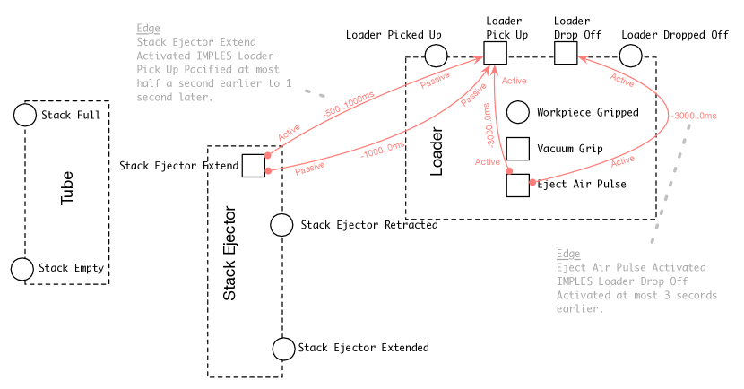
Figure 8: Avoidance topology

Each edge in the avoidance topology represents a temporal proximity relationship between two actuators: A state change in a first actuator (source node) leads to a state change in a second actuator (destination node). We assert that this must happen within some time range. The way we model this is by representing devices as nodes and the assertion as edges.

• Cause: the state change of the first actuator. This is done by annotating with the leading edge with the value the actuator state changes TO.

• Duration Range: One minimum and one maximum time duration.

• Effect: the state change of the second actuator. This is done by annotating with the leading edge with the value the actuator state changes TO.

The BeSpaceD encoding of these annotations use a TemporalConstraint as in Section 5.3.2. Below is an example of one such avoidance edge in BeSpaceD serialized to JSON (this edge is the top edge commented on in Figure 8):

{
    "type" : "EdgeAnnotated",
    "source" : {"type":"Component","id":"Stack Ejector Extend"},
    "target" : {"type":"Component","id":"Loader Pickup"},
    "annotation" : {
        "type": "FestoStateConstraint",
        "cause": {"type": "Active"},
        "durationRange": {
            "type":"TimeDurationRange",
            "minimum":{
                "type":"TimeDuration",
                "start":{"type": "SS Variable", "expression": {"type": "Active"}},
                "scalar":{"type": "SS Addition", "expression": [
                    {"type": "SS Variable", "expression": {"type": "Active"}},
                    {"type": "SS Constant", "expression": -500}
                    ]}
                },
            "maximum":{
                "type":"TimeDuration",
                "start":{
                    "type": "SS Variable",
                    "expression": {"type": "Active"}},
                "scalar":{
                    "type": "SS Addition",
                    "expression": [
                        {"type": "SS Variable", "expression": {"type": "Active"}},
                        {"type": "SS Constant", "expression": 1000}
                        ]
                    }
                }
            },
    "effect": {"type": "Passive"}}
}

5.4 Events

The model for live events from the food processing factory is built in layers of domain specific types that ultimately derive from BeSpaceD constructs. Figure 9 illustrates the BeSpaceD data structure for live events.

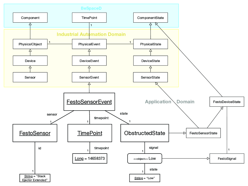
Figure 9: Example sensor event

The figure also shows the traits from the industrial automation domain to further illustrate the layers. The entity Low on the diagram is an immutable singleton object (in Scala) meaning the name refers to an object instance of a class with the same name as the object.

    case object Low  extends FestoSignal("Low" )

Types for sensors, actuators and parts are built from Component objects. Types for the state of these devices are built from ComponentState objects. And finally types for events are built from the core type in the industrial automation domain called PhysicalEvent (see Section 3.4).

Physical events are a composition of the previous two types plus a time point. The three key pieces of information are the object this event is scoped to, the time this event occurred and the state this object changed to. Below is an example of how to create a live event for the demonstrator plant. Apart from the time this constrction code matched the the illustration in Figure 9:

      val now = new GregorianCalendar()
      val timePoint = TimePoint(now.getTime.getTime)
      val event = FestoSensorEvent(
                         CapDispenser.StackEjectorExtended,
                         timePoint,
                         ObstructedLow
                         )

The state ObstructedLow is predefined in our application domain along with general light sensor states as follows:

      abstract class FestoLightSensorState(sig: FestoSignal)
               extends FestoSensorState(sig)
      class ObstructedState(sig: FestoSignal)
            extends FestoLightSensorState(sig)
      val ObstructedHigh = ObstructedState(High)
      val ObstructedLow = ObstructedState(Low)

5.5 Visualizing Topology and Events

We created a visualisation of live events from our food processing demonstrator in the context of a topology. A snapshot of an example visualisation can be seen in Figure 10.

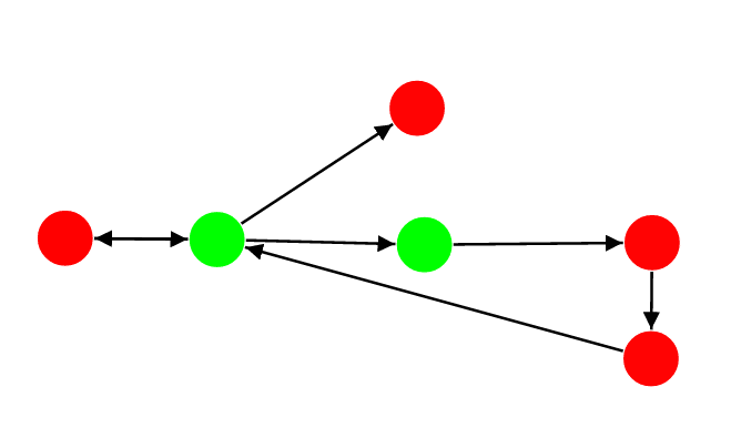
Figure 10: Example visualisation of topology and events

In this visualisation, a red node means the sensor is obstructed and a green node means it is not. This corresponds to the the state changes inferred from the incoming live events. The tool eStoreEd was used to create this visualisation.

6 Conclusion

We have presented domain specific constructs for industrial automation in our BeSpaceD modelling and reasoning framework. Furthermore, we presented some specific insights into the formalization of our food processing facility. This report continues a series of work, where we exemplify and highlight characteristics of our BeSpaceD framework.

Acknowledgement

We would like to thank Ian D. Peake, Lasith Fernando, James Harland, Huai Liu, Zoran Savic, and Yvette Wouters as well as our students for supporting us with the formalization work of the factory demonstrator.

References

- [1] The BeSpaceD development team. BeSpaceD repository https://bitbucket.org/bespaced/bespaced-2016
- [2] Jan Olaf Blech. An Example for BeSpaceD and its Use for Decision Support in Industrial Automation. http://arxiv.org/abs/1512.04656. arXiv.org, 2015.
- [3] Jan Olaf Blech, Lasith Fernando, Keith Foster, Abhilash G and Sudarsan Sd. Spatio-temporal Reasoning and Decision Support for Smart Energy Systems. Emerging Technologies and Factory Automation (ETFA), IEEE, 2016.
- [4] Jan Olaf Blech, Keith Foster. Operators for Space and Time in BeSpaceD. http://arxiv.org/abs/1602.08809. arXiv.org, 2016
- [5] Jan Olaf Blech, Ian Peake, Heinz Schmidt, Mallikarjun Kande, Srini Ramaswamy, Sudarsan Sd, Venkateswaran Narayanan. Collaborative Engineering through Integration of Architectural, Social and Spatial Models. Emerging Technologies and Factory Automation (ETFA), IEEE, 2014.
- [6] Jan Olaf Blech, Ian Peake, Heinz Schmidt, Mallikarjun Kande, Akilur Rahman, Srini Ramaswamy, Sudarsan SD, Venkateswaran Narayanan. Efficient Incident Handling in Indus- trial Automation through Collaborative Engineering. Emerging Technologies and Factory Au- tomation (ETFA), IEEE, 2015.
- [7] Jan Olaf Blech and Heinz Schmidt. Towards Modeling and Checking the Spatial and Interaction Behavior of Widely Distributed Systems. Improving Systems and Software Engineering Conference, Melbourne, 2013.
- [8] Jan Olaf Blech, Heinz Schmidt. BeSpaceD: Towards a Tool Framework and Methodology for the Specification and Verification of Spatial Behavior of Distributed Software Component Systems, http://arxiv.org/abs/1404.3537.arXiv.org, 2014.
- [9] Jan Olaf Blech, Maria Spichkova, Ian Peake, Heinz Schmidt. Cyber-Virtual Systems: Simulation, Validation & Visualization. Evaluation of Novel Approaches to Software Engineering. Lisbon, ISBN 978-989-758-030-7, pages 218-225, 2014.
- [10] J. Chen, A. G. Cohn, D. Liu, S. Wang, J. Ouyang, and Q. Yu. A survey of qualitative spatial representations. The Knowledge Engineering Review, 30(01):106–136, 2015.
- [11] A. G. Cohn and S. M. Hazarika. Qualitative spatial representation and reasoning: An overview. Fundamenta informaticae, 46(1-2):1–29, 2001.
- [12] Keith Foster, Jan Olaf Blech. Example Data Sets and Collections for BeSpaceD Ex- plained. http://arxiv.org/abs/1608.00433. arXiv.org, 2016.
- [13] Fenglin Han, Jan Olaf Blech, Peter Herrmann and Heinz Schmidt. Model-based Engineering and Analysis of Space-aware Systems Communicating via IEEE 802.11. CompSac’15, IEEE, 2015.
- [14] James Harland, Jan Olaf Blech, Ian Peake, Luke Trodd. Formal Behavioural Models to Facilitate Distributed Development and Commissioning in Industrial Automation. Evaluation of Novel Approaches to Software Engineering (ENASE), COLAFORM Track, ISBN 978-989-758-189-2, pages 363-369, ScitePress, 2016.
- [15] Peter Herrmann, Alexander Svae, Henrik Heggelund Svendsen, Jan Olaf Blech. Collaborative Model-based Development of a Remote Train Monitoring System. Evaluation of Novel Approaches to Software Engineering, COLAFORM Track, 2016.
- [16] Simon Hordvik, Kristoffer Øseth, Jan Olaf Blech, Peter Herrmann. A Methodology for Model-based Development and Safety Analysis of Transport Systems. Evaluation of Novel Approaches to Software Engineering, 2016.
- [17] Frank Alexander Kraemer, Vidar Slatten, and Peter Herrmann. Tool support for the rapid composition, analysis and implementation of reactive services. Journal of Systems and Software, vol. 82, issue 12, pp. 2068-2080, Elsevier, 2009.
- [18] Ian D. Peake, Jan Olaf Blech, Edward Watkins, Stefan Greuter, Heinz W. Schmidt. The Virtual Experiences Portals – A Reconfigurable Platform for Immersive Visualization. 3rd International Conference on Augmented Reality, Virtual Reality and Computer Graphics (SALENTO AVR 2016), Springer, 2016.
- [19] D. A. Randell, Z. Cui, and A. G. Cohn. A spatial logic based on regions and connection. In Proceedings of the 3rd International Conference on Knowledge Representation and Reasoning, pages 165–176, 1992.