Advanced Data Reduction for the MUSE Deep Fields

Abstract

The Multi Unit Spectroscopic Explorer (MUSE) is an integral-field spectrograph operating in the visible wavelength range, and installed at the Very Large Telescope (VLT). The official MUSE pipeline is available from ESO. However, for the data reduction of the Deep Fields program (Bacon et al., in prep.), we have built a more sophisticated reduction pipeline, with additional reduction tasks, to extend the official pipeline and produce cubes with fewer instrumental residuals.

1 Introduction

MUSE is composed of 24 Integral-field spectrographs (IFU) operating in the visible wavelength. The instrument has a field of view of $1^{\prime}\times 1^{\prime}$ sampled at 0.2 arcsec, an excellent image quality (limited by the 0.2 arcsec sampling), a large simultaneous spectral range (4650–9300 Ȧ), a medium spectral resolution ($R\simeq 3000$) and a very high throughput.

The data reduction for this instrument is the process which converts raw data from the 24 CCDs into a combined datacube (with two spatial and one wavelength axis) which is corrected for instrumental and atmospheric effects. Since the instrument consists of many subunits (24 integral-field units, each slicing the light into 48 parts, i.e. 1152 regions with a total of almost 90000 spectra per exposure), this task requires many steps and is computationally expensive, in terms of processing speed, memory usage, and disk input/output. This can be achieved with the MUSE standard pipeline (Weilbacher et al. 2012), with is available from ESO (http://www.eso.org/sci/software/pipelines/muse/muse-pipe-recipes.html).

For the data reduction of the Deep Fields program (Bacon et al., in prep.), we have built a more sophisticated reduction pipeline, with additional data-reduction tasks, to extend the official one. We use this pipeline to process the exposures we have for these two fields:

Hubble Deep Field South (HDFS)

As one of the commissioning activities MUSE acquired single deep field in the HDFS. A $1^{\prime}\times 1^{\prime}$ field was observed to a 26.5h depth (53 $\times$ 1800 s). Bacon et al. (2015) present a full description of the data, which is also available on the Muse Science website (http://muse-vlt.eu/science/hdfs-v1-0/).

Hubble Ultra Deep Field (UDF)

The MUSE-Deep GTO survey has observed a 9 field mosaic that covers the UDF. This $3^{\prime}\times 3^{\prime}$ field has been observed to a depth of $\sim$10h (in exposures of 1500 s each). In addition, there is also an extra-deep $1^{\prime}\times 1^{\prime}$ portion of the mosaic that reaches $\sim$31h. This data will be appear in Bacon at al. (in prep.), the redshifts in Brinchmann et al. (in prep.) and the full catalogue in Inami at al. (in prep.).

Section 2 describes the data reduction pipeline that we implement to process the data. Section 3 describes the additional tasks that are used to reduce the data.

Figure 1.: Example of a Ly$\alpha$ emitter detected in the HDFS data cube.

2 Data Processing

When there are many exposures ($\sim$300 in our cases, $\sim$2.2Tb of raw data), it becomes infeasible to manually keep track of everything. Instead it is crucial to build automated and reproducible procedures for tasks like associating the multiple calibration files needed for a given observation. That’s why we have built a custom data-reduction system with a database that contains all of the information from the science and calibration exposures. This lets us reliably identify files, based on criteria such as time offsets or temperature differences.

Running all the reduction steps for all the exposures requires a lot of computing time and produces a lot of files (several Tb per reduction). To keep track of the results and output logs of the different steps and versions, we have built a processing pipeline based on several key components:

• doit: having a dozen of tasks to run for each exposure, one of the key points was to be able to track the state of the processing for each task. doit (http://pydoit.org) is a task management and automation tool, open source and written in Python. doit is a flexible tool which allows to define task dependencies, actions and targets. doit remember the tasks execution, and can run multiple tasks in parallel.

• SQlite: a database used to store information about all the files (raw, calibration, outputs) and the runs.

• Jupyter notebook: used for the quality analysis. It is an easy way to explore the data and plot the relevant information, while running directly onto the computing server and accessed remotely. Once the notebook is ready, we use it to generate HTML pages for each exposure.

3 Additional reduction steps

The pipeline works well for the general case, but several things can be improved with some additional reduction steps (Figure 2). Most of these steps can be done with the recently released MPDAF Python package (Piqueras et al. 2017).

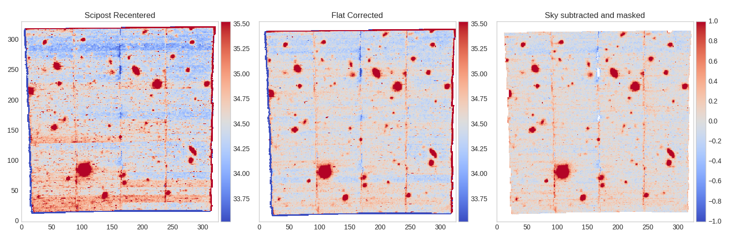
Figure 2.: Reduction of an HDFS exposure: white-light image after running the pipeline (left), after recentering and correction of the slices level (middle), after the sky subtraction with ZAP and masking the edges (right).

Flat fielding

We developed an automatic flat-fielding procedure, which computes and apply a correction to the slices level, using the sky level as a reference (thus this needs to be done before the sky subtraction). Available in MPDAF:

p = mpdaf.drs.PixTable(’PIXTABLE.fits’)  # open pixtable
mask = p.mask_column(maskfile=maskfile)  # mask sources
sky = p.sky_ref(pixmask=mask)            # compute the sky spectrum
cor = p.subtract_slice_median(sky, mask) # correct the slices level
p.write(’PIXTABLE-COR.fits’)             # save corrected pixtable
cor.write(’AUTOCALIB.fits’)              # save statistics
        

Sky subtraction

Sky subtraction is performed with ZAP (Soto et al. 2016), a high precision sky subtraction tool, also released this year. The method uses Principal Component Analysis to isolate the residual features and remove them from the observed datacube (Figure 3). ZAP can also be run in addition to the sky subtraction of the MUSE pipeline.

Masking

Various masking steps are applied, to remove instrumental artifacts that cannot be corrected. This is done both on pixtables and datacubes.

Combination

Exposures combination applied on data cubes, which allow to run additional steps on the cubes before combining them. This is also part of MPDAF. Several combination algorithm are available (mean, median, sigma clipping, with the CubeList class), and it can be used to create a mosaic (CubeMosaic).

PSF estimation

We developed a way to estimate the PSF parameters, calibration factors and pointing offsets, using HST as a reference: for each HST band, the image is resampled to the MUSE resolution, and fitted to a MUSE image computed on the same band (Figure 4).

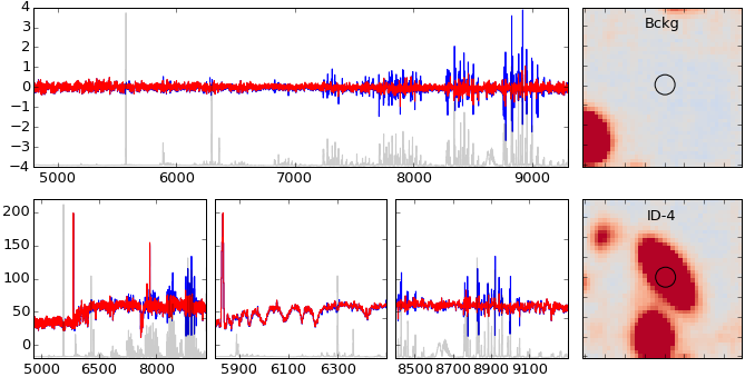
Figure 3.: Spectra after ZAP (red) compared to the MUSE pipeline (blue)

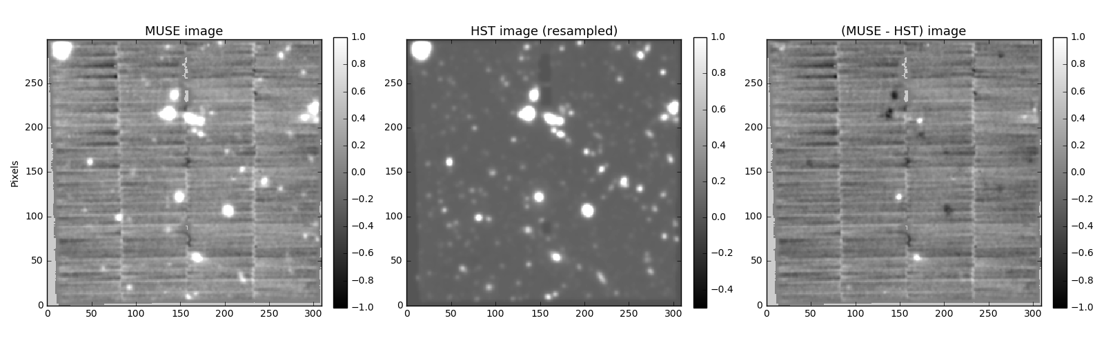
Figure 4.: PSF estimation: fitted MUSE image, fitted HST image, and residual.

4 Conclusion

The additional data reduction tasks presented here allow us to produce final (combined) cubes with reduced sky residuals, smaller background variations, and fewer instrumental effects, which is useful for the next steps: sources detection, redshifts estimation, and the scientific exploitation. Most of the steps are available in the recently released MPDAF Python package (Piqueras et al. 2017).

Acknowledgments

RB acknowledges support from the ERC advanced grant MUSICOS.

References

- Bacon et al. (2015) Bacon, R., , et al. 2015, A&A, 575, A75. 1411.7667
- Piqueras et al. (2017) Piqueras, L., Conseil, S., Shepherd, M., & Bacon, R. 2017, in ADASS XXVI, edited by TBD (San Francisco: ASP), vol. TBD of ASP Conf. Ser., TBD
- Soto et al. (2016) Soto, K. T., Lilly, S. J., Bacon, R., Richard, J., & Conseil, S. 2016, MNRAS, 458, 3210. 1602.08037
- Weilbacher et al. (2012) Weilbacher, P. M., Streicher, O., Urrutia, T., Jarno, A., Pécontal-Rousset, A., Bacon, R., & Böhm, P. 2012. URL http://dx.doi.org/10.1117/12.925114