Better Higgs Measurements Through Information Geometry

Abstract

Information geometry can be used to understand and optimize Higgs measurements at the LHC. The Fisher information encodes the maximum sensitivity of observables to model parameters for a given experiment. Applied to higher-dimensional operators, it defines the new physics reach of any LHC signature. We calculate the Fisher information for Higgs production in weak boson fusion with decays into tau pairs and four leptons, and for Higgs production in association with a single top quark. In a next step we analyze how the differential information is distributed over phase space, which defines optimal event selections. Conversely, we consider the information in the distribution of a subset of the kinematic variables, showing which production and decay observables are the most powerful and how much information is lost in traditional histogram-based analysis methods compared to fully multivariate ones.

I Introduction

After its experimental discovery higgs ; discovery the Higgs boson and its properties have immediately become one of the most important and active fields of searches for physics beyond the Standard Model at the LHC. In the Lagrangian language of fundamental physics, the Higgs properties can be described by a continuous and high-dimensional parameter space, for instance in terms of Wilson coefficients in an effective field theory (EFT) eftfoundations ; eftorig ; eftreviews . One of the main features of moving from simple coupling modifications to higher-dimensional operators is that we can now include kinematic distributions in these searches higgs_fit ; yr4 . A common challenge of all Higgs analyses is how to navigate the vast family of phase-space distributions.

Responding to the overwhelming amount of search strategies, we expect the LHC collaborations to focus more and more on high-level statistical tools, including hypothesis tests based on multivariate analysis with machine learning or the matrix element method statistics ; kyle_review . Historically, these tools compare two discrete hypotheses, and applying them to continuous, high-dimensional parameter spaces is computationally expensive. Only recently, machine learning techniques have been extended to include inference on such continuous high-dimensional parameter spaces machine_learning . With these capabilities, it becomes increasingly important to be able to effectively characterize the information contained in these distributions. We present an approach based on information geometry information-geometry , intrinsically designed to study continuous parameter spaces of arbitrary dimensionality without the need for any discretization of the hypothesis. We use this to compare and improve Higgs measurement strategies.

Our central object is the Fisher information matrix. Through the Cramér-Rao bound it determines the maximum knowledge on model parameters that we can derive from an observation cramer-rao ; information-applications . In that sense the Cramér-Rao bound for the Fisher information plays a similar role as the Neyman-Pearson lemma neyman-pearson plays for a discrete hypothesis test and the log-likelihood ratio: it allows us to define and to compute the best possible outcome of any multivariate black-box analysis kyle_review ; madmax1 . In addition, the Fisher information matrix defines a metric in the space of model parameters, which not only provides an intuitive geometric picture, but also gives us a handle on the linearization of the observable in terms of new physics effects.

When we apply our information geometry framework to Higgs physics, in particular to analyses of the dimension-6 Higgs Lagrangian, we can tackle questions of the kind:

• What is the maximum precision with which we can measure continuous model parameters?

• How is the information distributed over phase space?

• How much of the full information is contained in a given set of distributions?

• Which role do higher-dimensional corrections in the EFT expansion play?

We demonstrate our approach using three examples: Higgs production in weak boson fusion (WBF) dave_thesis with its tagging-jet kinematics tagging is well known to probe many aspects of the Higgs-gauge coupling structure phi_jj . Focusing on the WBF production kinematics we first analyze its combination with a Higgs decay to tau leptons wbf_tau . This will for example allow us to estimate how much of the entire information on higher-dimensional operators is typically included in the leading tagging jet distributions. Combining WBF production with a Higgs decay to $ZZ^{*}$ pairs we can test how much additional information is included in the decay distributions. Conceptually, this contrasts two ways to constrain the same effective Lagrangian via large momentum flow through the relevant vertices or via precision observables higgs_fit . Finally, we will test how useful Higgs production in association with a single top top_higgs is for a dimension-6 operator analysis.

In a set of appendices we give a worked-out simple example for our approach, explain how we compute the Fisher information, show more information on our example processes, indicate how systematic or theory uncertainties can be included, and discuss the relation of our approach to standard log-likelihood ratios.

II Information geometry and Cramér-Rao bound

At the LHC, we typically use a set of possibly correlated event rates $\mathbf{x}$ to measure a set of model parameters. Those can, for example, be a vector of Higgs couplings with the unknown true value $\mathbf{g}$. These Higgs couplings define a continuous, high-dimensional model space. The outcome of the measurement is an estimator for the couplings $\hat{\mathbf{g}}$ that follows a probability distribution $f(\hat{\mathbf{g}}|\mathbf{g})$. For an unbiased estimator its expectation value is equal to its true value,

$$\bar{g}_{i}\equiv E\left[\hat{g}_{i}\middle|\mathbf{g}\right]=g_{i}\,.$$ (1)

Our argument can be trivially extended to biased estimators. The variance, or for more than one model parameter the covariance matrix

$$C_{ij}(\mathbf{g})\equiv E\left[(\hat{g}_{i}-\bar{g}_{i})(\hat{g}_{j}-\bar{g}_{j})\middle|\mathbf{g}\right]\,,$$ (2)

provides a measure of the precision of the measurement. For a set of uncorrelated measurements the covariance matrix is a diagonal matrix made of the individual variances.

The relation $f(\mathbf{x}|\mathbf{g})$ between the measurement $\mathbf{x}$ and assumed true parameters $\mathbf{g}$ can be extracted from Monte-Carlo and detector simulations. If we know it, we can describe the reach of a measurement using the Fisher information matrix

$$I_{ij}(\mathbf{g})\equiv-E\left[\frac{\partial^{2}\log f(\mathbf{x}|\mathbf{g})}{\partial g_{i}\,\partial g_{j}}\middle|\mathbf{g}\right]\,.$$ (3)

The Cramér-Rao bound cramer-rao states that the covariance matrix in Eq. (2) is bounded from below by the inverse Fisher information: the smallest achievable uncertainty is then given by

$$C_{ij}\geq(I^{-1})_{ij}\,.$$ (4)

Large entries in the Fisher information indicate directions in model space which can be measured well. Eigenvectors with eigenvalue zero are blind directions. Fortunately, the Fisher information is invariant under a reparametrization of the observables $\mathbf{x}$, and transforms covariantly under a reparametrization of the model parameters $\mathbf{g}$.

After removing blind directions, the Fisher information is a symmetric and positive definite rank-two tensor and defines a Riemannian metric on the model space information-geometry . This allows us define a local as well a as global distance measure in model space,

$$d_{\text{local}}(\mathbf{g}_{b};\mathbf{g}_{a}) =\sqrt{(\mathbf{g}_{a}-\mathbf{g}_{b})_{i}\,I_{ij}(\mathbf{g}_{a})\,(\mathbf{g}_{a}-\mathbf{g}_{b})_{j}}$$

$$d(\mathbf{g}_{b},\mathbf{g}_{a}) =\min_{\mathbf{g}(s)}\;\int_{s_{a}}^{s_{b}}ds\;\sqrt{\frac{dg_{i}(s)}{ds}\,I_{ij}(\mathbf{g}(s))\,\frac{dg_{j}(s)}{ds}}\,,$$ (5)

where the global distance is the length of a geodesic (the curve that minimizes the distance). Contours of constant distances define optimal error ellipsoids. The distance tracks how (un-)likely it is to measure $\hat{\mathbf{g}}=\mathbf{g}_{b}$ given the true value $\mathbf{g}=\mathbf{g}_{a}$. If the estimator is distributed according to a multivariate Gaussian around the true value, the local distance values directly correspond to the difference in $\hat{\mathbf{g}}$ and $\mathbf{g}_{a}$ measured in standard deviations.

A typical LHC measurement includes an observed total number of events $n$, distributed over possible phase space positions $\mathbf{x}$. The probability distribution in Eq. (3) factorizes kyle_review ; madmax1

$$f(\mathbf{x}_{1},\dots,\mathbf{x}_{n}|\mathbf{g})=\operatorname{Pois}(n|L\sigma(\mathbf{g}))\;\prod_{i=1}^{n}f^{(1)}(\mathbf{x}_{i}|\mathbf{g})\,,$$ (6)

where $f^{(1)}(\mathbf{x}|\mathbf{g})$ is the normalized probability distribution for a single event populating the phase space position $\mathbf{x}$. This can be calculated for example with Monte-Carlo simulations. The total cross section is $\sigma(\mathbf{g})$, to be multiplied with the integrated luminosity $L$. The corresponding Fisher information is

$$I_{ij} =\frac{L}{\sigma}\;\frac{\partial\sigma}{\partial g_{i}}\,\frac{\partial\sigma}{\partial g_{j}}-L\,\sigma\;E\left[\frac{\partial^{2}\log f^{(1)}(\mathbf{x}|\mathbf{g})}{\partial g_{i}\,\partial g_{j}}\right]\,.$$ (7)

The Fisher information is additive when we combine phase-space regions. After integrating over the entire phase space, this full Fisher information defines the minimum covariance matrix possible.

Instead of integrating over the entire phase space, it is enlightening to study how the information is distributed in phase space. Consider the differential quantity $dI_{ij}/d\mathbf{v}$, where $\mathbf{v}$ is a kinematic variable like an invariant mass or angle calculated from $\mathbf{x}$. Here $I_{ij}$ uses all the information in $\mathbf{x}$, but we are able to study the distribution of the information with respect to $\mathbf{v}$. Such a distribution defines the important phase-space region for a measurement and should drive the design of event selections: it allows us to calculate the information loss from kinematic cuts, and to quantify the trade-off between signal purity and maximal information. Integrating over this differential information will reproduce the total Fisher information $I_{ij}$.

Conversely, if in Eq. (7) we replace the full phase space point $\mathbf{x}$ with a lower-dimensional set of kinematic variables $\mathbf{v}$, we will arrive at the information in this reduced set of kinematic variables. We refer to this as the information in distributions, and we will use this definition to identify how efficient analyses in terms of a small number of available kinematic distributions can be.

For our analysis we parametrize the Higgs properties in terms of dimension-6 operators eftfoundations ; eftorig ; eftreviews ,

$$\mathcal{L}_{\text{}}=\mathcal{L}_{\text{SM}}+\frac{f_{i}}{\Lambda^{2}}\mathcal{O}_{i}\quad\text{implying}\quad g_{i}=\frac{f_{i}\,v^{2}}{\Lambda^{2}}\,,$$ (8)

where the additional factor $v^{2}$ ensures that our parameters $\mathbf{g}$ are dimensionless, and the Standard Model corresponds to $\mathbf{g}=\mathbf{0}$. In Eq. (33) we see that the Fisher information around this point, $I_{ij}(\mathbf{0})$, only measures the linear terms in $\mathbf{g}\propto 1/\Lambda^{2}$ and is not sensitive to higher corrections. Dimension-6 squared contributions appear away from the Standard Model point and in the corresponding global distances. The difference between local and global distances thus provides a measure of the impact of $1/\Lambda^{4}$ contributions eft-edge .

III Weak-boson-fusion Higgs to taus

The first question we tackle with our information geometry approach is what we can learn about higher-dimensional operators from the non-trivial kinematics of weak-boson-fusion production. As a decay we include a simple fermionic two-body decay $H\to\tau\tau$ wbf_tau , see Fig. 1. For our proof of concept we stick to a parton-level analysis at leading order. The dominant irreducible backgrounds are QCD $Zjj$ production and electroweak $Zjj$ production, both with the decay $Z\to\tau\tau$, and Higgs production in gluon fusion with $H\to\tau\tau$.

Figure 1: Example Feynman diagram for weak-boson-fusion Higgs production with $H\to\tau\tau$. The red dot shows the Higgs-gauge interactions affected by the dimension-6 operators of our analysis.

We do not simulate tau decays, but multiply the rates with the branching ratios for the semi-leptonic di-tau mode and assume the di-tau system can be reconstructed with the collinear approximation with a realistic resolution for $m_{\tau\tau}$. Following the procedure outlined in Refs. madmax1 ; madmax2 , we smear the $m_{\tau\tau}$ distributions using a Gaussian (with width 17 GeV) for Higgs production and a double Gaussian (where the dominant component has a width of 13 GeV) for $Z$ production, estimated from Fig. 1a of Ref. Aad:2015vsa . The double Gaussian ensures an accurate description of the high-mass tail of the $Z$ peak around $m_{\tau\tau}=m_{H}$. Otherwise, no detector effects are included. We require loose cuts

$$p_{T,j} >20\ {\mathrm{GeV}}\qquad \qquad|\eta_{j}| <5.0\qquad \qquad\Delta\eta_{jj} >2.0$$

$$p_{T,\tau} >10\ {\mathrm{GeV}}\qquad \qquad|\eta_{\tau}| <2.5\,,$$ (9)

to include as much of phase space as possible.

The different QCD radiation patterns of electroweak and QCD signal and background processes are a key feature to separate the signal from the background tagging . We take it into account through approximate individual jet veto survival probabilities wbf_tau ,

$$\varepsilon^{\text{CJV}}_{\text{WBF $H$}}=0.71\qquad\qquad\varepsilon^{\text{CJV}}_{\text{EW $Z$}}=0.48\qquad\qquad\varepsilon^{\text{CJV}}_{\text{QCD $Z$}}=0.14\qquad\qquad\varepsilon^{\text{CJV}}_{\text{GF $H$}}=0.14\,.$$ (10)

Since our phase space $\mathbf{x}$ does not include any jets other than the two tagging jets, we are not sensitive to details of the central jet veto other than the relative survival probabilities and possible second-order effects that would correlate the veto with $\mathbf{x}$. After the event selection of Eq. (9) and applying the CJV efficiencies, the WBF Higgs signal of 53 fb in the SM faces a dominant QCD $Z$ background of 2.7 pb.

We consider five $CP$-even dimension-6 operators in the HISZ basis hisz ; higgs_fit ,

$$\mathcal{O}_{B} =i\frac{g}{2}\,(D^{\mu}\phi^{\dagger})(D^{\nu}\phi)\,B_{\mu\nu}\quad \quad\mathcal{O}_{W} =i\frac{g}{2}\,(D^{\mu}\phi)^{\dagger}\sigma^{k}(D^{\nu}\phi)\,W_{\mu\nu}^{k}$$

$$\mathcal{O}_{BB} =-\frac{g^{\prime 2}}{4}\,(\phi^{\dagger}\phi)\,B_{\mu\nu}\,B^{\mu\nu}\quad \quad\mathcal{O}_{WW} =-\frac{g^{2}}{4}\,(\phi^{\dagger}\phi)\,W^{k}_{\mu\nu}\,W^{\mu\nu\,k}$$

$$\mathcal{O}_{\phi,2} =\frac{1}{2}\,\partial^{\mu}(\phi^{\dagger}\phi)\,\partial_{\mu}(\phi^{\dagger}\phi)\,.$$ (11)

The first four operators introduce new Lorentz structures into Higgs-gauge interactions, which translate into changed kinematic shapes. The pure Higgs operator $\mathcal{O}_{\phi,2}$ leads to a universal rescaling of all single-Higgs couplings and otherwise only affects the Higgs self-coupling. Other operators that contribute to WBF Higgs production are tightly constrained by electroweak precision data or can be removed from the basis using field redefinitions power-to-the-data . The effect of $\mathcal{O}_{\phi,2}$ on gluon-fusion Higgs production is taken into account in our analysis, while the effects from $\mathcal{O}_{W}$ and $\mathcal{O}_{B}$ on the subleading electroweak $Zjj$ background are neglected.

III.1 Maximum precision on Wilson coefficients

Figure 2: Error ellipses defined by the Fisher information in the WBF $H\to\tau\tau$ channel. We show contours of local distance $d_{\text{local}}(\mathbf{g};\mathbf{0})$ (dashed) and global distance $d(\mathbf{g},\mathbf{0})$ (solid). The colored contours indicate distances of $d=1~{}...~{}5$. In grey we show example geodesics. The $g_{i}$ not shown are set to zero.

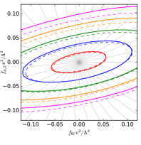
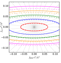
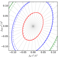
Following Eq. (8), our model space is spanned by five dimensionless parameters

$$\mathbf{g}=\frac{v^{2}}{\Lambda^{2}}\begin{pmatrix}[c]f_{\phi,2}\\ f_{W}\\ f_{WW}\\ f_{B}\\ f_{BB}\end{pmatrix}\,.$$ (12)

With these basis vectors we calculate the Fisher information for 13 TeV using a combination of MadGraph5 madgraph , MadMax madmax2 , and our own MadFisher algorithm, described in Appendix A.2. We absorb all particle identification and trigger efficiencies into a single universal $\varepsilon$ (which does not include the process-dependent CJV efficiencies). Then for our toy example we assume the integrated luminosity times universal efficiencies to be $L\cdot\varepsilon=30~{}\mathrm{fb}^{-1}$. We find

$$I_{ij}(\mathbf{0})=\begin{pmatrix}[r]3202.1&-625.3&-7.2&-34.8&0.3\\ -625.3&451.0&-109.5&23.3&-1.5\\ -7.2&-109.5&243.7&-5.5&2.8\\ -34.8&23.3&-5.5&4.1&-0.3\\ 0.3&-1.5&2.8&-0.3&0.1\end{pmatrix}\,.$$ (13)

The eigenvectors, ordered by the size of their eigenvalues, are

$$\mathbf{g}_{1}=\begin{pmatrix}[r]0.98\\ -0.21\\ 0.01\\ -0.01\\ 0.00\end{pmatrix}\quad\mathbf{g}_{2}=\begin{pmatrix}[r]-0.18\\ -0.79\\ 0.58\\ -0.04\\ 0.01\end{pmatrix}\quad\mathbf{g}_{3}=\begin{pmatrix}[r]0.12\\ 0.57\\ 0.81\\ 0.03\\ 0.01\end{pmatrix}\quad\mathbf{g}_{4}=\begin{pmatrix}[r]0.00\\ -0.05\\ 0.00\\ 1.00\\ -0.07\end{pmatrix}\quad\mathbf{g}_{5}=\begin{pmatrix}[r]0.00\\ -0.00\\ -0.01\\ 0.07\\ 1.00\end{pmatrix}\,.$$ (14)

The corresponding eigenvalues are $\left(3338,395,165,2.9,0.1\right)$, indicating that the WBF process has very different sensitivities to the five operators: $\mathcal{O}_{\phi,2}$ can be most strongly constrained and is weakly correlated with $\mathcal{O}_{W}$. It is followed by the strongly correlated $\mathcal{O}_{W}$-$\mathcal{O}_{WW}$ plane. The sensitivity to $\mathcal{O}_{B}$ and $\mathcal{O}_{BB}$, which only play a role in subleading $Z$-mediated production diagrams, is much smaller and shows very little correlation with each other and everything else.

We visualize our results as contours of the local and global distances defined in Eq. (5) for slices of parameter space in Fig. 2. First, the contours show the maximum precision that can be attained in a measurement in this process. Without taking into account systematic uncertainties, an optimal measurement will probe the $\mathcal{O}_{\phi,2}$ direction with $\Delta g\approx 0.02$, translating into $\Lambda/\sqrt{f_{\phi,2}}\approx 1.8$ TeV. The $\mathcal{O}_{W}$ and $\mathcal{O}_{WW}$ directions can optimally be probed at the $\Delta g\approx 0.05$ or $\Lambda/\sqrt{f_{\phi,2}}\approx 1.1$ TeV level.

Comparing the local and global distances provides some insight into the role of $\mathcal{O}\!\left(1/\Lambda^{4}\right)$ effects, as discussed before. At $d=1,2$ the differences are small, signaling that an optimal measurement will be dominated by the linearized dimension-6 amplitudes. On the other hand, analyses based on less luminosity or requiring more stringent exclusion criteria (translating into larger distances) will only probe new physics scales closer to the electroweak scale, in which case the squared dimension-6 terms will have a larger effect.

III.2 Differential information

The fact that the Fisher information is additive across different phase-space regions means that we can consider the differential information with respect to phase space ($dI_{ij}/d\mathbf{x}$) or a specific kinematic variable ($dI_{ij}/d\mathbf{v}$). In Fig. 3 we show the differential cross sections of the signal and dominant background process for typical kinematic distributions and compare it to the differential information. More distributions are shown in Appendix A.3.

Figure 3: Distribution of the Fisher information in the WBF $H\to\tau\tau$ channel (shaded red). We also show the normalized SM signal (solid black) and QCD $Z$+jets (dotted grey) rates. The dashed blue line shows the effect of an exaggerated $f_{W}\,v^{2}/\Lambda^{2}=0.5$. The last bin is an overflow bin.

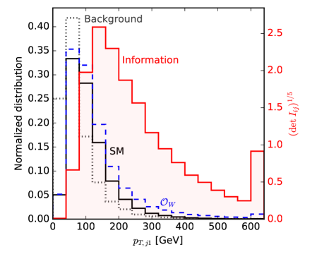
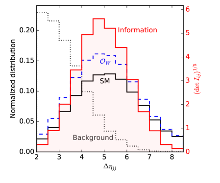
Obviously, the signal-to-background ratio improves for large invariant masses of the tagging jets and towards $m_{\tau\tau}$ values around the Higgs mass. The information is larger in these phase-space regions, independent of the direction in model space. On the other hand, most of our dimension-6 operators include derivatives, leading to an increasing amplitude with momentum transfer through the gauge-Higgs vertex. This momentum flow is not observable, but the transverse momenta of the tagging jets and the Higgs boson are strongly correlated with it eft-edge . Indeed most of the information on higher-dimensional operators comes from the high-energy tail of $p_{T,j_{1}}$.

The rapidity difference between the tagging jets indicates a trade-off between these two effects: on the one hand, at larger rapidity distances the signal-to-background ratio clearly improves phi_jj . On the other hand, the largest effects from dimension-6 operators appear at smaller $\Delta\eta_{jj}$, again driven by the larger momentum transfer eft-edge . In the right panel of Fig. 3 we see that the information on these operators comes from $\Delta\eta_{jj}=3\dots 7$. Tight cuts with the aim to remove backgrounds lose a sizable fraction of the information on dimension-6 operators.

III.3 Information in distributions

Figure 4: Information from histograms compared to the full information (black) in the WBF $H\to\tau\tau$ channel, shown as contours $d_{\text{local}}(\mathbf{g};\mathbf{0})=1$. We include $p_{T,j_{1}}$, $\Delta\phi_{jj}$, their naive combination assuming no mutual information, and their two-dimensional histogram. The $g_{i}$ not shown are set to zero.

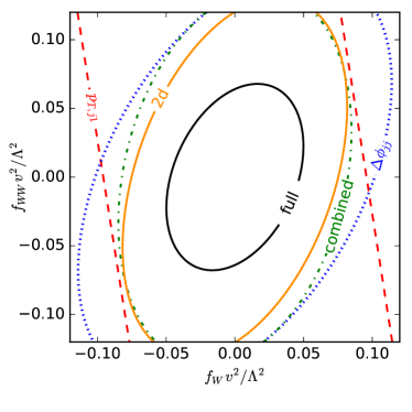
While the integrated, fully differential information defined in Eq. (7) provides us with optimal experimental results, it remains to be shown that we can access it in practice. Recent proposals using machine learning for high-dimensional likelihood fits aim to tackle exactly this problem machine_learning . Regardless, a relevant question is how much of this maximum information is retained in simple one-dimensional or two-dimensional distributions of standard kinematic observables $\mathbf{v}$.

In the presence of backgrounds, a histogram-based analysis first requires a stringent event selection, either based on traditional kinematic cuts or on a multivariate classifier. First, we choose the WBF cuts

$$105~{}{\mathrm{GeV}}<m_{\tau\tau}<165~{}{\mathrm{GeV}}\qquad p_{T,j_{1}}>50~{}{\mathrm{GeV}}\qquad m_{jj}>1~{}{\mathrm{TeV}}\qquad\Delta\eta_{jj}>3.6\,.$$ (15)

This improves the signal-to-background ratio to approximately unity, but at the cost of losing discrimination power. Eventually, a histogram-based analysis will benefit from optimizing this selection, for instance foregoing the simple cuts for a multivariate approach, going beyond the scope of this demonstration. Based on this selection, we analyze the distributions

• $p_{T,\tau_{1}}$ with bin size 25 GeV up to 500 GeV and an overflow bin;

• $m_{\tau\tau}$ with bin size 5 GeV in the allowed range of $105~{}...~{}165~{}{\mathrm{GeV}}$;

• $p_{T,\tau\tau}$ with bin size 50 GeV up to 800 GeV and an overflow bin;

• $p_{T,j_{1}}$ with bin size 50 GeV up to 800 GeV and an overflow bin;

• $m_{jj}$ with bin size 250 GeV up to 4 TeV and an overflow bin;

• $\Delta\eta_{jj}$ with bin size $0.5$ up to $8.0$ and an overflow bin;

• $\Delta\phi_{jj}=\phi_{j_{\eta<0}}-\phi_{j_{\eta>0}}$ phi_jjs with bin size $2\pi/20$;

• $\Delta\eta_{\tau\tau,j1}$ with bin size $0.5$ up to $8.0$ and an overflow bin;

• $\Delta\phi_{\tau\tau,j1}$ with bin size $\pi/10$.

Figure 5: Fisher information for the WBF $H\to\tau\tau$ channel exploiting the full phase space, after the cuts in Eq. (15), and for several kinematic distributions. The top panel shows the eigenvalues, the colors denote the composition of the corresponding eigenvectors. The right axis translates the eigenvalues into a new physics reach for the corresponding combination of Wilson coefficients. In the bottom panel we show the determinants of the Fisher information restricted to $\mathcal{O}_{\phi,2}$, $\mathcal{O}_{W}$, and $\mathcal{O}_{WW}$, normalized to the full information. Again, the right axis translates them into a new physics reach.

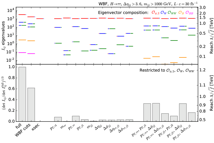
Figure 4 demonstrates that virtuality measures such as the transverse momentum of the leading tagging jet mostly constrain $\mathcal{O}_{W}$, while angular correlations between the jets are more sensitive to $\mathcal{O}_{WW}$. Stringent constraints on the full operator space can only be achieved by combining the information in these (or more) distributions, ideally in a two-dimensional histogram.

In Fig. 5 we extend our comparison to the information in all of the above distributions. The top panel shows the eigenvalues of the individual information matrices, and the colors indicate which operators the corresponding eigenvectors are composed of. This allows us to see which operators can be measured well in which distributions, and where blind (or flat) directions arise. In the lower panel we compare the determinants, providing a straightforward measure of the information in distributions that is invariant under basis rotations.

In general, single differential cross sections probe individual directions in phase space well, but always suffer from basically blind directions. To maximize the constraining power on all operators we need to combine virtuality measures and angular correlations. Even then there is a substantial difference to the maximum information in the process: the combined analysis of jet transverse momenta and $\Delta\phi_{jj}$ has a new physics reach in the $\mathcal{O}_{\phi,2}$-$\mathcal{O}_{W}$-$\mathcal{O}_{WW}$ space of $0.9~{}{\mathrm{TeV}}$, compared to $1.2~{}{\mathrm{TeV}}$ for the fully differential cross section. Under our simplistic assumptions this corresponds to roughly three times more data. Half of this loss in constraining power is due to information in background-rich regions discarded by the WBF cuts, and half is due to non-trivial kinematics not captured by the double differential distributions.

In light of the large amount of information discarded by the WBF cuts in Eq. (15), we repeat this comparison with an alternative multivariate event selection. Instead of cutting on standard kinematic observables, we select all events in “signal-like” phase-space regions, defined as those with a larger expected SM WBF rate than expected background rates,

$$\frac{\sigma_{\text{SM WBF}}\;f^{(1)}(\mathbf{x}|\text{SM WBF})}{\sigma_{\text{backgrounds}}\;f^{(1)}(\mathbf{x}|\text{backgrounds})}=\frac{\Delta\sigma_{\text{SM WBF}}(\mathbf{x})}{\Delta\sigma_{\text{backgrounds}}(\mathbf{x})}>1\,.$$ (16)

We then calculate the information in the same distributions as before.

Figure 6: Fisher information for the WBF $H\to\tau\tau$ channel exploiting the full phase space, after the likelihood-based event selection in Eq. (16), and for several kinematic distributions. Except for the initial cuts, the plot is analogous to Fig. 5.

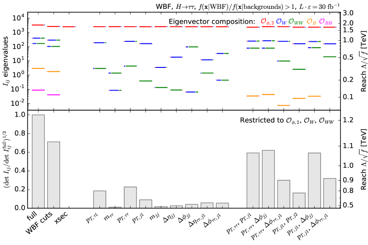
As shown in Fig. 6, the cut in Eq. (16) defines a sample with little background contamination without sacrificing much discrimination power. One-dimensional and two-dimensional distributions can extract information on the operators more reliably than after the kinematic event selection in Eq. (15). A combined measurement of the jet transverse momenta and $\Delta\phi_{jj}$ is now able to probe new physics scales of up to 1.1 GeV compared to 1.2 GeV for the fully multivariate approach, corresponding to $70\%$ more data.

IV Weak-boson-fusion Higgs to four leptons

Another question we can approach with information geometry is how much the non-trivial decay mode $H\to 4\ell$ adds to the WBF production analyzed in Sec. III. For this particularly clean channel, shown in Fig. 7, the backgrounds are not the limiting factor, so we omit them for our toy study. For instance, in the relevant phase-space region the cross section of the dominant irreducible $ZZ^{*}\,jj$ background is over an order of magnitude smaller than the SM Higgs signal. This also allows us to avoid smearing the $m_{4\ell}$ distribution. At parton level we apply the generator-level cuts

$$p_{T,j} >20\ {\mathrm{GeV}}\qquad \qquad|\eta_{j}| <5.0$$

$$p_{T,\ell} >10\ {\mathrm{GeV}}\qquad \qquad|\eta_{\ell}| <2.5\;,$$ (17)

with $\ell=e,\mu$. The SM cross section after these cuts is 0.36 fb.

Figure 7: Example Feynman diagram for weak-boson-fusion Higgs production with $H\to 4\ell$. The red dots show the Higgs-gauge interactions affected by the dimension-6 operators of our analysis.

IV.1 Maximum precision on Wilson coefficients

Again we study the five-dimensional space of CP-even Wilson coefficients given in Eq. (12). For increased luminosity, $L\cdot\varepsilon=100~{}\mathrm{fb}^{-1}$, we find the SM information

$$I_{ij}(\mathbf{0})=\begin{pmatrix}[r]144.3&-27.3&-11.5&-1.6&-0.7\\ -27.3&50.9&-9.1&6.7&-0.2\\ -11.5&-9.1&36.9&-1.2&1.0\\ -1.6&6.7&-1.2&1.9&-0.1\\ -0.7&-0.2&1.0&-0.1&0.1\end{pmatrix}$$ (18)

with the eigenvectors

$$\mathbf{g}_{1}=\begin{pmatrix}[r]0.96\\ -0.25\\ -0.08\\ -0.02\\ 0.00\end{pmatrix}\quad\mathbf{g}_{2}=\begin{pmatrix}[r]-0.16\\ -0.79\\ 0.58\\ -0.11\\ 0.02\end{pmatrix}\quad\mathbf{g}_{3}=\begin{pmatrix}[r]0.21\\ 0.54\\ 0.81\\ 0.09\\ 0.02\end{pmatrix}\quad\mathbf{g}_{4}=\begin{pmatrix}[r]0.02\\ 0.14\\ 0.01\\ -0.99\\ 0.04\end{pmatrix}\quad\mathbf{g}_{5}=\begin{pmatrix}[r]0.00\\ -0.00\\ -0.03\\ 0.04\\ 1.00\end{pmatrix}\,.$$ (19)

and the eigenvalues $\left(152.4,52.8,27.8,1.0,0.0\right)$.

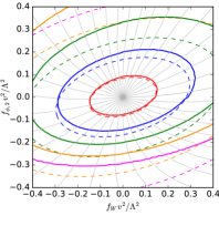
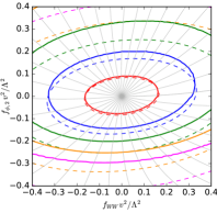
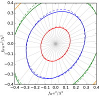
The Fisher information approach allows us to directly compare this outcome to our earlier results for WBF production with $H\to\tau\tau$ in Eq. (13), or to calculate the combined information in these two channels by simply adding their Fisher information matrices after rescaling them to the same luminosity. Clearly, the $\tau\tau$ channel contains significantly more information on all operators. The decay $H\to 4\ell$ does not even increase the sensitivity to $\mathcal{O}_{B}$ or $\mathcal{O}_{BB}$, both of them are still basically blind directions. We visualize the information geometry in the remaining directions in Fig. 8. The differences between local and global distances are much larger than in the $H\to\tau\tau$ channel. This is because the tiny $H\to 4\ell$ branching fraction decreases the new physics reach and with it the hierarchy of scales in our effective Lagrangian. This means that the squared dimension-6 amplitudes are numerically more relevant.

Figure 8: Error ellipses defined by the Fisher information in the WBF $H\to 4\ell$ channel. We show contours of local distance $d_{\text{local}}(\mathbf{g};\mathbf{0})$ (dashed) and global distance $d(\mathbf{g},\mathbf{0})$ (solid). The colored contours indicate distances of $d=1~{}...~{}5$. In grey we show example geodesics. The $g_{i}$ not shown are set to zero.

IV.2 Production vs decay kinematics

Figure 9: Information in the WBF $H\to 4\ell$ channel from including dimension-6 operators only in the production vertex (red), only in the decay vertex (blue), and both (black). The information is visualized as local contours $d_{\text{local}}(\mathbf{g};\mathbf{0})=1$. The $g_{i}$ not shown are set to zero.

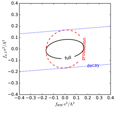
Focusing on the question how the decay analysis improves our global information, we disentangle the effects on the production and decay vertices in Fig. 9. As well known for the LHC, the production-side analysis benefits from a large momentum flow through the Higgs vertex, while the momentum flow through the decay vertices is bounded by the Higgs mass (neglecting off-shell phase space regions). For momentum-dependent operators this disadvantage is not compensated by the complex $H\to 4\ell$ decay kinematics. Consequently, the Higgs decay only improves the reach in the $\mathcal{O}_{\phi,2}$ direction, corresponding to a change in the total rate. This operator also affects many other total Higgs rates, so we conclude that the complex $H\to 4\ell$ kinematics does not play a significant role as part of a global analysis.

Figure 10: Fisher information for the WBF $H\to 4\ell$ channel, based on the full kinematics and on individual kinematic distributions. The top panel shows the eigenvalues, the colors denote the composition of the corresponding eigenvectors. The right axis translates the eigenvalues into a new physics reach for the corresponding combination of Wilson coefficients. In the bottom panel we show the determinants of the Fisher information restricted to $\mathcal{O}_{\phi,2}$, $\mathcal{O}_{W}$, and $\mathcal{O}_{WW}$, normalized to the full information. Again, the right axis translates them into a new physics reach.

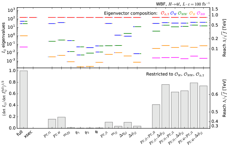
In complete analogy to Fig. 5 for the WBF production, we compare the information in different distributions for $CP$-even operators in Fig. 10. The standard tagging jet observables are complemented by five observables characterizing the $4\ell$ decay kinematics,

• $p_{T,\ell_{1}}$;

• $p_{T,4\ell}$;

• $m_{Z_{2}}$ for the lower-mass reconstructed $Z$ boson;

• $\cos\theta_{1}=\hat{p}_{\ell^{-}_{1}}\cdot\hat{p}_{Z_{2}}\Big{|}_{Z_{1}}$ defined in terms of unit-3-vectors $\hat{p}$, and analogously $\cos\theta_{2}$;

• $\cos\Phi=(\hat{p}_{\ell^{-}_{1}}\times\hat{p}_{\ell^{+}_{1}})\cdot(\hat{p}_{\ell^{-}_{2}}\times\hat{p}_{\ell^{+}_{2}})$, defined in the $ZZ$ or Higgs rest frame phi_jj .

In all cases we use at least ten bins and include underflow and overflow bins where applicable.

In our quantitative analysis we find similar patterns as in the $\tau\tau$ mode. The key observables are again transverse momenta and jet angular correlations. Without the complication of removing backgrounds efficiently, the combined analysis of these variables comes close to the maximum information: a two-dimensional histogram of jet transverse momenta and $\Delta\phi_{jj}$ probes new physics scales up to 650 GeV, while for a fully differential analysis the maximum probed new physics scale is close to 700 GeV. Under our assumptions, this difference roughly corresponds to 25% more data. The decay kinematics and its angular observables do not help significantly or change the picture qualitatively. This shows again how much the sensitivity of the decay vertices to dimension-6 operators is limited by the restriction of the momentum flow to the Higgs mass. This is not accidental: the reason behind this role of the momentum dependence is that for all operators shown in Eq. (12) with the exception of $\mathcal{O}_{\phi,2}$, gauge invariance forces us to include the field strength tensor instead of the gauge boson field, automatically introducing a momentum dependence.

V Higgs plus single top

Our final example is Higgs production with a single top with $H\to\gamma\gamma$ and a hadronic top decay. As shown in Fig. 11, diagrams where the Higgs is radiated off a $W$ boson interfere destructively with diagrams with a top-Higgs coupling, making this channel a direct probe of the sign of the top Yukawa coupling top_higgs . We stick to a parton-level analysis at leading order in the five-flavor scheme. For our toy example we include only one of the dominant backgrounds, single top production with two photons, and in particular ignore the multi-jet background. The subleading $t\bar{t}\,\gamma\gamma$ background populates qualitatively different phase-space regions from the single-top signal and can be supressed with an appropriate event selection Kling:2012up . We smear the $m_{\gamma\gamma}$ distribution of the signal process with a Gaussian of width 1.52 GeV estimated from Fig. 6b of Ref. CMS:2016zjv , and do not include any other detector effects. Our basic event selection requires

$$p_{T,j} >20\ {\mathrm{GeV}}\quad \quad|\eta_{j}| <5.0\quad \quad\Delta R_{jj} >0.4\quad \quad 152\ {\mathrm{GeV}} <m_{bjj}<192\ {\mathrm{GeV}}$$

$$p_{T,\gamma} >10\ {\mathrm{GeV}}\quad \quad|\eta_{\gamma}| <2.5\quad \quad\Delta R_{\gamma j},\Delta R_{\gamma\gamma} >0.4\quad \quad 120\ {\mathrm{GeV}} <m_{\gamma\gamma}<130\ {\mathrm{GeV}}\,,$$ (20)

leading to a SM $tH$ cross section of 0.10 fb and a background of 0.22 fb.

Figure 11: Example Feynman diagrams for Higgs production with a single top, not resolving the loop-induced $H\gamma\gamma$ coupling. The red dots show the Higgs interactions affected by the dimension-6 operators of our analysis.

We consider four $CP$-even dimension-6 operators

$$\mathcal{O}_{W} =i\frac{g}{2}\,(D^{\mu}\phi)^{\dagger}\sigma^{k}(D^{\nu}\phi)\,W_{\mu\nu}^{k}\qquad \qquad\mathcal{O}_{t\phi} =(\phi^{\dagger}\phi)\,(\mkern 1.5mu\overline{\mkern-1.5muQ\mkern-1.5mu}\mkern 1.5mu_{3}\tilde{\phi}t_{R})+\text{h.c.}$$

$$\mathcal{O}_{WW} =-\frac{g^{2}}{4}\,(\phi^{\dagger}\phi)\,W^{k}_{\mu\nu}\,W^{\mu\nu\,k}\qquad \qquad\mathcal{O}_{\phi,2} =\frac{1}{2}\,\partial^{\mu}(\phi^{\dagger}\phi)\,\partial_{\mu}(\phi^{\dagger}\phi)\,.$$ (21)

The operators $\mathcal{O}_{W}$ and $\mathcal{O}_{WW}$ affect the production amplitudes where the Higgs couples to a $W$, while $\mathcal{O}_{t\phi}$ re-scales the top Yukawa coupling. Both, $\mathcal{O}_{WW}$ and $\mathcal{O}_{\phi,2}$ also affect the $H\to\gamma\gamma$ decay.

V.1 Maximum precision on Wilson coefficients

Figure 12: Error ellipses defined by the Fisher information in Higgs plus single top production. We show contours of local distance $d_{\text{local}}(\mathbf{g};\mathbf{0})$ (dashed) and global distance $d(\mathbf{g},\mathbf{0})$ (solid). The colored contours indicate distances of $d=1~{}...~{}5$. In grey we show example geodesics. The $g_{i}$ not shown are set to zero.

We calculate the Fisher information in terms of the dimensionless parameters

$$\mathbf{g}=\frac{v^{2}}{\Lambda^{2}}\begin{pmatrix}[c]f_{\phi,2}\\ f_{W}\\ f_{WW}\\ f_{t\phi}\end{pmatrix}$$ (22)

for 13 TeV and an integrated luminosity times efficiencies of $L\cdot\varepsilon=300~{}\mathrm{fb}^{-1}$ and find

$$I_{ij}(\mathbf{0})=\begin{pmatrix}[r]80.1&-18.7&-957.0&13.2\\ -18.7&32.6&221.7&27.0\\ -957.0&221.7&11446.1&-146.0\\ 13.2&27.0&-146.0&150.3\end{pmatrix}\,.$$ (23)

The eigenvectors are

$$\mathbf{g}_{1}=\begin{pmatrix}[r]0.08\\ -0.02\\ -1.00\\ 0.01\end{pmatrix}\qquad\mathbf{g}_{2}=\begin{pmatrix}[r]0.00\\ -0.23\\ -0.01\\ -0.97\end{pmatrix}\qquad\mathbf{g}_{3}=\begin{pmatrix}[r]-0.02\\ 0.97\\ -0.02\\ -0.23\end{pmatrix}\qquad\mathbf{g}_{4}=\begin{pmatrix}[r]1.00\\ 0.02\\ 0.08\\ -0.01\end{pmatrix}$$ (24)

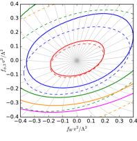
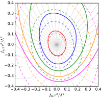
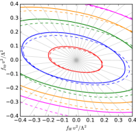
with corresponding eigenvalues $\left(11532,155,21.3,0.1\right)$. The best constrained direction is along $\mathcal{O}_{WW}$ and corresponds to the combination of Wilson coefficients that affects the $H\to\gamma\gamma$ decay in addition to production effects, which will already be tightly constrained once a $tH$ measurement is feasible. The orthogonal direction in the $\mathcal{O}_{\phi,2}$-$\mathcal{O}_{WW}$ plane is for all practical purposes blind. Even with the assumed sizeable event rate corresponding to 300 $\mathrm{fb}^{-1}$, the sensitivity to $\mathcal{O}_{W}$ and $\mathcal{O}_{t\phi}$ is limited, with some mixing between the two operators.

We visualize this maximum sensitivity to dimension-6 operators in Fig. 12. With the exception of $\mathcal{O}_{WW}$, an optimal measurement can probe all operators at the $\Delta g\approx 0.1\dots 0.2$ level, equivalent to $\Lambda/\sqrt{f_{\phi,2}}\approx 600\dots 750$ GeV. There are large differences between local and global distances already at the $d=2$ level, implying that a measurement of this channel will always be sensitive to the squared dimension-6 terms.

V.2 Differential information

Figure 13: Distribution of the Fisher information in the Higgs plus single top channel (shaded red). We also show the normalized SM signal (solid black) and single-top background (dotted grey) rates. The dashed blue line shows the effect of $f_{t\phi}\,v^{2}/\Lambda^{2}=0.2$. The last bin is an overflow bin.

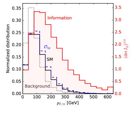
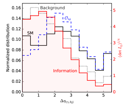
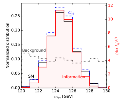
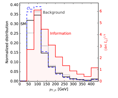
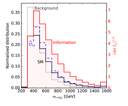
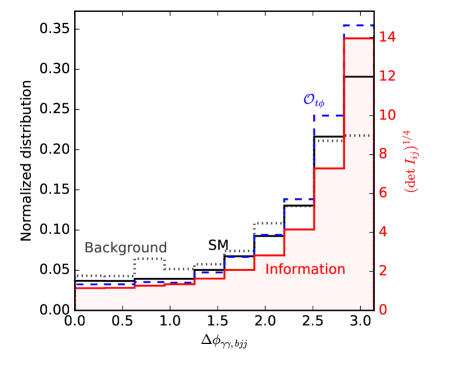
In Fig. 13 we show the distribution of this information over phase space. More distributions are shown in Appendix A.3. As expected, the information is concentrated in the $m_{\gamma\gamma}\sim m_{H}$ peak and in the high-energy tails of transverse momenta. Studying angular correlations between the Higgs system and the top decay products, we find that the region $\Delta\eta_{\gamma\gamma,bjj}\lesssim 3$ contains a lot of discrimination power.

V.3 Information in distributions

In a next step, we compare this full information to the reduced information in one-dimensional and two-dimensional distributions of kinematic observables. We now require harder cuts

$$p_{T,j_{1}}>50~{}{\mathrm{GeV}}\qquad p_{T,\gamma}>50,~{}30~{}{\mathrm{GeV}}\qquad 122~{}{\mathrm{GeV}}<m_{\gamma\gamma}<128~{}{\mathrm{GeV}}\,,$$ (25)

which reduces the background to the level of the signal. We then analyze the distributions top_higgs ; Kling:2012up

• $p_{T,\gamma_{1}}$ with bin size 25 GeV up to 400 GeV and an overflow bin;

• $m_{\gamma\gamma}$ with bin size 1 GeV in the allowed range of $123~{}...~{}127~{}{\mathrm{GeV}}$;

• $p_{T,\gamma\gamma}$ with bin size 40 GeV up to 600 GeV and an overflow bin;

• $\Delta\phi_{\gamma\gamma}$ with bin size $\pi/10$;

• $p_{T,j_{1}}$ with bin size 40 GeV up to 400 GeV and an overflow bin;

• $p_{T,b}$ with bin size 40 GeV up to 400 GeV and an overflow bin;

• $p_{T,bjj}$ with bin size 40 GeV up to 600 GeV and an overflow bin;

• $\Delta\phi_{\gamma\gamma,b}$ with bin size $\pi/10$;

• $\Delta\eta_{\gamma\gamma,b}$ with bin size $0.5$ up to $5.0$ and an overflow bin;

• $m_{\gamma\gamma bjj}$ with bin size 100 GeV up to 1500 GeV and an overflow bin;

• $p_{T,\gamma\gamma bjj}$ with bin size 40 GeV up to 400 GeV and an overflow bin;

• $\Delta\phi_{\gamma\gamma,bjj}$ with bin size $\pi/10$;

• $\Delta\eta_{\gamma\gamma,bjj}$ with bin size $0.5$ up to $5.0$ and an overflow bin.

Figure 14: Information from histograms compared to the full information (black), shown as contours $d_{\text{local}}(\mathbf{g};\mathbf{0})=1$. We include $p_{T,\gamma\gamma}$, $\Delta\eta_{\gamma\gamma,bjj}$, their naive combination assuming no mutual information, and their two-dimensional histogram. The $g_{i}$ not shown are set to zero.

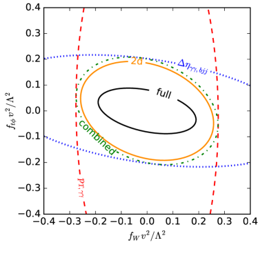
As in the WBF case, different observables probe different Wilson operators. Figure 14 shows that the di-photon transverse momentum constrains mostly the $\mathcal{O}_{W}$ direction, while the rapidity separation between the Higgs and top systems is more sensitive to $\mathcal{O}_{t\phi}$.

Figure 15: Fisher information for the Higgs plus single top channel exploiting the full phase space, after the cuts in Eq. (25), and for several kinematic distributions. The top panel shows the eigenvalues, the colors denote the composition of the corresponding eigenvectors. The right axis translates the eigenvalues into a new physics reach for the corresponding combination of Wilson coefficients. In the bottom panel we show the determinants of the Fisher information restricted to $\mathcal{O}_{\phi,2}$, $\mathcal{O}_{W}$, and $\mathcal{O}_{t\phi}$, normalized to the full information. Again, the right axis translates them into a new physics reach.

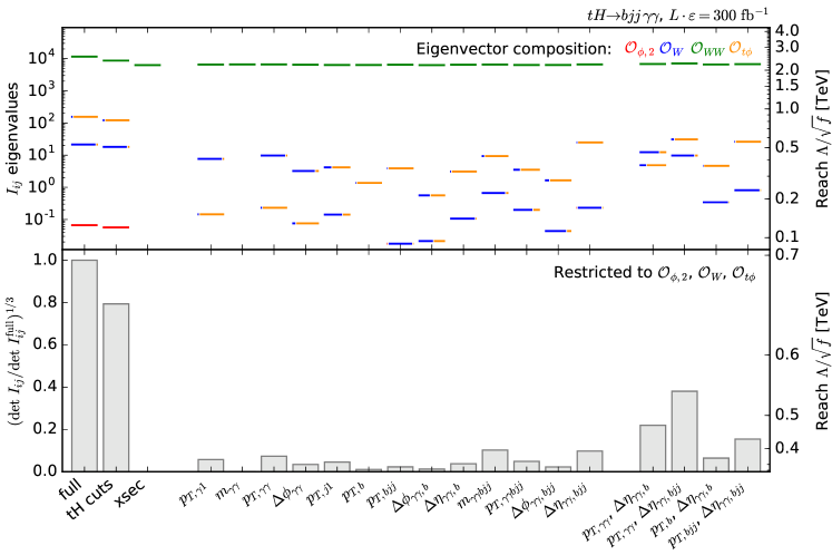
In Fig. 15 we compare the eigenvalues, eigenvectors and determinants of the information matrices in all of the above distributions. We confirm that the photon observables mostly probe changes in the Higgs-gauge coupling from $\mathcal{O}_{W}$, while a rescaled top Yukawa will be visible in the properties of the top decay products. Distributions of the properties of the $b$ jet consistently contain significantly less information than the corresponding distributions for the reconstructed top system. The rapidity difference between the $\gamma\gamma$ system and the reconstructed top provides a particularly good probe of this operator top_higgs . Combining this variable with the transverse momentum of the $\gamma\gamma$ system we can probe new physics scales in the $\mathcal{O}_{\phi,2}$-$\mathcal{O}_{W}$-$\mathcal{O}_{t\phi}$ space around 550 GeV, compared to 700 GeV for the fully differential cross section. This corresponds to almost three times more data under our simplifying assumptions.

VI Conclusions

We have used information geometry to calculate the maximum sensitivity of Higgs measurements to dimension-6 operators, to understand the structure of the observables, and to discuss how to improve these measurements. Our approach is based on the Fisher information matrix, which according to the Cramér-Rao bound defines the maximum precision that can be achieved in a measurement. Unlike traditional multivariate analysis techniques, it is designed for continuous, high-dimensional parameter spaces like effective field theories. We have demonstrated how the Fisher information can be reliably calculated using Monte-Carlo techniques.

Going beyond global statements, the Fisher information can be studied differentially to understand how the discriminating power is distributed over phase space, which helps guide event selection strategies. Moreover, we can also calculate the information contained in subsets of kinematic distributions. This helps us determine which observables are the most powerful, and allows us to compare the constraining power in conventional analyses with one or two variables to that in more complex multivariate analyses.

Our first testing ground was Higgs production in weak boson fusion with decays into a tau pair or into four leptons. Crucial information comes from the high-energy tails as well as from angular correlations between jets. Decay kinematics hardly adds any information, since the momentum flow is limited by the Higgs mass and gauge invariance forces us to include operators with a momentum dependence. Tight cuts on the rapidity separation of the tagging jets throw away a large amount of discrimination power. Under idealized conditions, conventional analyses based on a simple event selection and standard kinematic distributions can probe new physics scales around $900~{}{\mathrm{GeV}}$ in the early phase of Run II. Multivariate analyses have the potential to significantly enhance the sensitivity and probe new physics scales of up to $1.2~{}{\mathrm{TeV}}$.

In Higgs production with a single top we find that kinematic properties of the Higgs decay products and observables in the top system provide orthogonal information. The transverse momenta of the di-photon system as well as the rapidity separation of the $\gamma\gamma$ and $bjj$ systems are powerful observables. But even with HL-LHC data these distributions are only sensitive to new physics scales around $550~{}{\mathrm{GeV}}$, while a multivariate analysis might be able to probe scales up to $700~{}{\mathrm{GeV}}$.

To summarize, information geometry provides a powerful and intuitive tool that can help understand the phenomenology of models with a continuous, high-dimensional parameter space, and in turn can be used to optimize measurement strategies. We have demonstrated this approach in different Higgs channels for dimension-6 operators, but it can easily be translated to other processes and models.

Acknowledgments

We would like to thank Juan Gonzalez-Fraile for many fruitful discussions and sharing his model file for some of the dimension-6 operators. We are grateful to Peter Schichtel for helping us to set up and use MadMax. We would also like to acknowledge Ben Allanach’s early interest in pursuing information geometry in the context of supersymmetry.

JB is funded by the DFG through the Graduiertenkolleg Particle physics beyond the Standard Model (GRK 1940). KC is supported through NSF ACI-1450310 and PHY-1505463. The work of FK is supported by NSF under Grant PHY-1620638. TP is supported by the DFG Forschergruppe New Physics at the LHC (FOR 2239). The authors acknowledge support by the state of Baden-Württemberg through bwHPC.

Appendix A Additional results

A.1 A simple example

As a simple example we study the Fisher information in a number of rates $n_{c}$ measured in various Higgs channels $c$. In the absence of systematic uncertainties they follow Poisson statistics,

$$f(\mathbf{n}|\boldsymbol{\nu})=\prod_{c}\operatorname{Pois}(n_{c}|\nu_{c})=\prod_{c}\,\frac{\nu_{c}^{n_{c}}e^{-\nu_{c}}}{n_{c}!}\,.$$ (26)

We can calculate the Fisher information in terms of the Poisson mean $\boldsymbol{\nu}$ as

$$\frac{\partial\log f}{\partial\nu_{c}}=\frac{n_{c}}{\nu_{c}}-1\qquad\qquad\frac{\partial^{2}\log f}{\partial\nu_{c}\partial\nu_{c^{\prime}}}=-\frac{\delta_{cc^{\prime}}\,n_{c}}{\nu_{c}^{2}}\qquad\qquad I_{cc^{\prime}}\equiv-E\left[\frac{\partial^{2}\log f}{\partial\nu_{c}\partial\nu_{c^{\prime}}}\middle|\boldsymbol{\nu}\right]=\frac{\delta_{cc^{\prime}}}{\nu_{c}}\,.$$ (27)

If we express the expected count rates in terms of model parameters $g_{i}$, the Fisher information becomes

$$I_{ij}=\sum_{c}\frac{1}{\nu_{c}}\,\frac{\partial\nu_{c}}{\partial g_{i}}\,\frac{\partial\nu_{c}}{\partial g_{j}}\,.$$ (28)

The matrix $\partial\nu_{c}/\partial g_{i}$ is determined by selection requirements, detector acceptance, and efficiencies. In the $\kappa$ framework that only scales cross sections and branching ratios, the matrix $\partial\nu_{c}/\partial g_{i}$ is trivial to calculate in closed form. For each channel this matrix is singular, which means it measures one direction in parameter space and is blind to all others. At least as many channels as parameters are required to make the combined information in Eq. (28) non-singular and remove all blind directions (assuming the channels do not provide degenerate information, i. e. the same eigenvectors in the Fisher information).

For illustration, we consider the case where we want to measure one coupling $g$ in one channel with the expected number of events

$$\nu=L\left(\sigma_{S}+\sigma_{B}\right)=Lg^{2}\sigma_{0}+L\sigma_{B}\;.$$ (29)

The Fisher information is then

$$I=4L\,\frac{g^{2}\sigma_{0}^{2}}{g^{2}\sigma_{0}+\sigma_{B}}=\frac{4L}{g^{2}}\,\frac{\sigma_{S}^{2}}{\sigma_{S}+\sigma_{B}}\,.$$ (30)

According to the Cramér-Rao bound, the standard deviation of any unbiased estimator $\hat{g}$ is at least

$$\frac{\Delta\hat{g}}{g}\geq\frac{1}{g\,\sqrt{I}}=\frac{1}{2\,\sqrt{L}}\,\frac{\sqrt{\sigma_{S}+\sigma_{B}}}{\sigma_{S}}\,.$$ (31)

The three terms show how the sensitivity to $g$ profits from the square in the cross section, the square-root dependence on the statistics, and the dependence on the signal-to-background ratio.

A.2 The MadFisher algorithm

We calculate the Fisher information in Eq. (7) with Monte-Carlo methods. With

$$\int\!dx\;f^{(1)}(x)\to\sum_{\text{events k}}\Delta\sigma_{k}/\sigma$$ (32)

we find

$$I_{ij}(\mathbf{g})=\sum_{\text{events }k}\frac{L}{\Delta\sigma_{k}(\mathbf{g})}\frac{\partial\Delta\sigma_{k}(\mathbf{g})}{\partial g_{i}}\,\frac{\partial\Delta\sigma_{k}(\mathbf{g})}{\partial g_{j}}\,,$$ (33)

requiring the differential cross sections and their derivatives as input.

We first generate event samples for a number of benchmark parameters with MadMax madmax2 . This add-on to MadGraph 5 madgraph allows us to simultaneously calculate differential rates for different parameter points using the same phase-space grid. Our FeynRules feynrules model file of the relevant dimension-6 operators does not truncate operator effects at $\mathcal{O}\!\left(1/\Lambda^{2}\right)$. MadMax requires fixed renormalization and factorization scales, which we set following Ref. yr4 . To keep the calculation times manageable, we restrict some processes to the dominant sub-processes, for instance to initial-state $u$ and $d$ quarks in the WBF case. We then normalize the Higgs rates to the LHC HXS WG recommendations for the total cross section yr4 , calculating the effect of the different acceptance regions with MadGraph 5. Background processes are simply rescaled to MadGraph predictions.

A morphing technique allows us to calculate the differential cross sections and their derivatives at arbitrary positions in parameter space morphing . The effect of $\mathcal{O}_{\phi,2}$ and systematic rate uncertainties (see Sec. A.4) is taken into account analytically. The contributions from the other operators are decomposed into a number of basis components and can be exactly reconstructed from a set of simulated benchmark points. Our example processes require up to 70 such basis components (in the WBF $H\to 4\ell$ case).

We can then easily calculate the Fisher information according to Eq. (33). Finally, global distances as in Eq. (5) are calculated in analogy to free fall in general relativity: a starting point and a set of directions in parameter space define the initial conditions, from which we numerically calculate distances along curves defined by the geodesic equation.

A.3 Additional distributions

Figure 16: Distribution of the Fisher information in the WBF $H\to\tau\tau$ channel (shaded red). We also show the normalized SM signal (solid black) and QCD $Z$+jets (dotted grey) rates. The dashed blue line shows the effect of an exaggerated $f_{W}\,v^{2}/\Lambda^{2}=0.5$ ($f_{WW}\,v^{2}/\Lambda^{2}=0.5$ in the bottom right panel). The first (last) bins are underflow (overflow) bins.

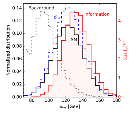
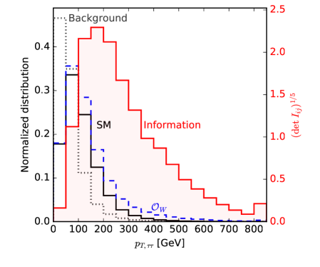
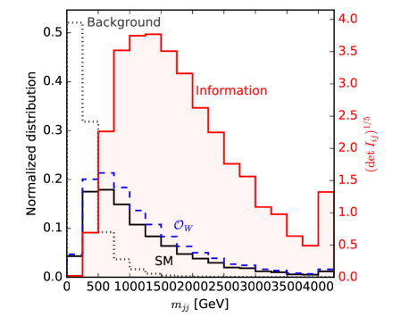
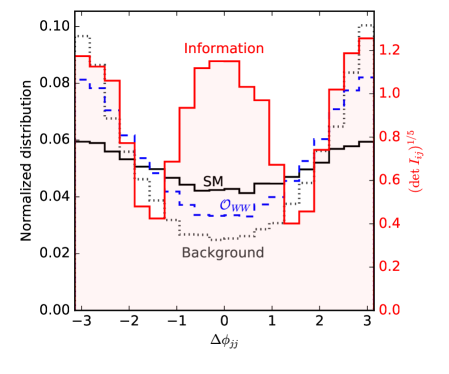
In Fig. 16 we show the distribution of the differential information in the WBF $H\to\tau\tau$ channel over various kinematic variables. Figure 17 contains similar distributions for the Higgs plus single top channel.

Figure 17: Distribution of the Fisher information in the Higgs plus single top channel (shaded red). We also show the normalized SM signal (solid black) and single-top background (dotted grey) rates. The dashed blue line shows the effect of $f_{t\phi}\,v^{2}/\Lambda^{2}=0.2$. The first (last) bins are underflow (overflow) bins.

A.4 Systematic uncertainties

Our information geometry approach can easily be extended to include systematic and theory uncertainties. The parameter space then consists of nuisance parameters $\nu_{i}$ in addition to the Wilson coefficients, and constraint terms are added to the likelihood. If for instance the $k$th parameter is a nuisance parameter with a Gaussian constraint term with width $\sigma_{k}$, the additional term in the Fisher information reads

$$I_{ij}(\mathbf{g},\boldsymbol{\nu})=\dots+\frac{\delta_{ik}\delta_{jk}}{\sigma_{k}^{2}}\,.$$ (34)

This also applies to a log-normal constraint through reparametrization of $\nu$. Local and global distances now refer to combined theory and nuisance parameters $(\mathbf{g},\boldsymbol{\nu})$.

We define a profiled local distance between two points $\mathbf{g}_{b}$ and $\mathbf{g}_{a}$

$$d_{\text{profiled}}(\mathbf{g}_{b},\mathbf{g}_{a})=\min_{\boldsymbol{\nu}}\;d_{\text{local}}((\mathbf{g}_{b},\boldsymbol{\nu});(\mathbf{g}_{a},\mathbf{0}))\,.$$ (35)

Equivalently, we can define a profiled Fisher information matrix. Assuming the last parameter to be the only nuisance parameter, the Fisher information matrix has the form

$$I_{ij}=\begin{pmatrix}[c]I^{\text{theory}}&\mathbf{m}\\ \mathbf{m}^{T}&n\end{pmatrix}$$ (36)

where $I^{\text{theory}}$ is the information matrix restricted to the theory parameters, the vector $\mathbf{m}$ describes the mixing between theory and nuisance parameter, and $n$ is the component that only affects the nuisance parameters. Technically described by the parallel projection of an ellipsoid, the projected Fisher information is given by

$$I_{\text{profiled}\,ij}=I^{\text{theory}}_{ij}-\frac{m_{i}m_{j}}{n}\,.$$ (37)

Figure 18: Effects of Gaussian uncertainties of $5\%$ and $10\%$ on the total signal rate. In the left panel we show the expected error ellipse $d_{\text{local}}((g,\nu);\mathbf{0})=1$ in the plane spanned by a physical parameter and the nuisance parameter $\nu$ rescaling the signal rate. In the right panel we show the error ellipses in the $\mathcal{O}_{W}$-$\mathcal{O}_{\phi,2}$ plane after profiling over this systematic uncertainty.

Figure 19: Fisher information for the WBF $H\to\tau\tau$ channel profiled over a $10\%$ signal rate uncertainty. We compare the information for the full phase space, after the cuts in Eq. (15), and for several kinematic distributions. The top panel shows the eigenvalues, the colors denote the composition of the corresponding eigenvectors. The right axis translates the eigenvalues into a new physics reach for the corresponding combination of Wilson coefficients. In the bottom panel we show the determinants of the Fisher information restricted to $\mathcal{O}_{\phi,2}$, $\mathcal{O}_{W}$, and $\mathcal{O}_{WW}$, normalized to the full information. Again, the right axis translates them into a new physics reach.

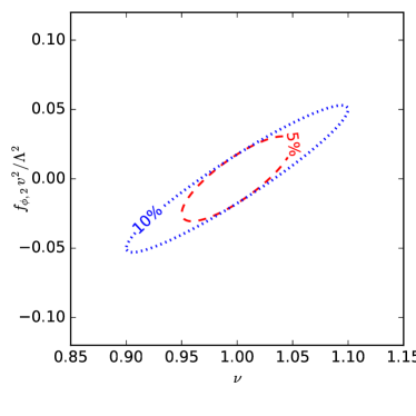
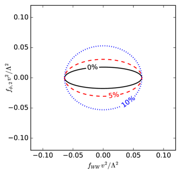
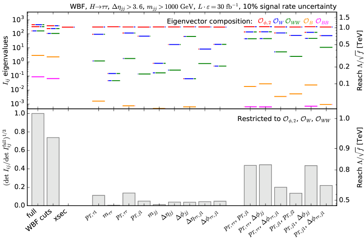
We demonstrate this for WBF Higgs production in the $\tau\tau$ mode in Fig. 18. We assign a $5\%$ or $10\%$ Gaussian uncertainty on the overall signal rate, representing for instance missing higher orders, pdf or efficiency uncertainties. This significantly reduces the information in the total rate, and thus mostly the expected precision in the $\mathcal{O}_{\phi,2}$ direction. In Fig. 19 we show how the information in various distributions is affected by such an uncertainty. The new physics reach in the $\mathcal{O}_{\phi,2}$ direction is reduced by 800 GeV.

A.5 Likelihood ratios and Fisher distance

There is some subtlety in the relationship between standard likelihood ratio tests and the Fisher distance. We anticipate that the confidence intervals in $\mathbf{g}$ will continue to be based on likelihood ratio tests. While both are invariant to reparametrization of $\mathbf{g}$, non-linear terms in $\mathbf{g}$ that lead to curvature in the information geometry can break the one-to-one relationship between the expected value of the log-likelihood ratio and the Fisher information distance.

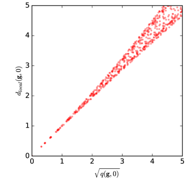
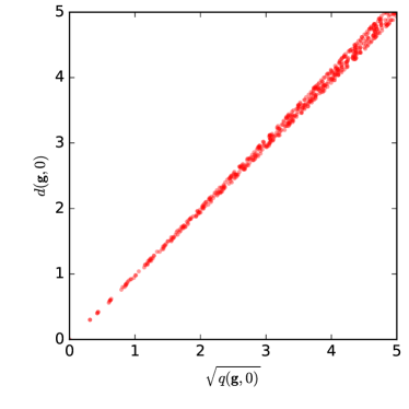
In Fig. 20 we compare the two tools. As an example, we study WBF Higgs production in the $\tau\tau$ mode and sample parameter points $\mathbf{g}$ in the $\mathcal{O}_{W}$-$\mathcal{O}_{WW}$ plane. For each of these points we calculate the local and global distance from the SM defined by the Fisher information, as well as the expected log-likelihood ratio

$$q(\mathbf{g}_{b},\mathbf{g}_{a})\equiv-2\,E\left[\log\frac{f(\mathbf{x}|\mathbf{g}_{b})}{f(\mathbf{x}|\mathbf{g}_{a})}\middle|\mathbf{g}_{a}\right]\,.$$ (38)

For small significance deviations, the local and especially the global distances are almost exactly equal to the expected likelihood ratio, with differences only becoming visible around the $3\sigma$ level. This demonstrates that different statistical tools probe the same physics and can be chosen based on convenience.

Figure 20: Comparison of the local (left) and global (right) distances defined by the Fisher information with the expected local likelihood ratio. We use WBF Higgs production in the $\tau\tau$ mode and sample parameter points in the $\mathcal{O}_{W}$-$\mathcal{O}_{WW}$ plane.

References

- (1) P. W. Higgs, Phys. Lett. 12, 132 (1964); P. W. Higgs, Phys. Rev. Lett. 13, 508 (1964); F. Englert and R. Brout, Phys. Rev. Lett. 13, 321 (1964).
- (2) G. Aad et al. [ATLAS Collaboration], Phys. Lett. B 716, 1 (2012) [arXiv:1207.7214 [hep-ex]]; S. Chatrchyan et al. [CMS Collaboration], Phys. Lett. B 716, 30 (2012) [arXiv:1207.7235 [hep-ex]].
- (3) S. Weinberg, Phys. Lett. B 91, 51 (1980); S. R. Coleman, J. Wess and B. Zumino, Phys. Rev. 177, 2239 (1969); C. G. Callan, Jr., S. R. Coleman, J. Wess and B. Zumino, Phys. Rev. 177, 2247 (1969).
- (4) C. J. C. Burges and H. J. Schnitzer, Nucl. Phys. B 228, 464 (1983); C. N. Leung, S. T. Love and S. Rao, Z. Phys. C 31, 433 (1986); W. Buchmüller and D. Wyler, Nucl. Phys. B 268, 621 (1986).
- (5) For reviews see e. g. M. S. Bilenky and A. Santamaria, Nucl. Phys. B 420, 47 (1994) [arXiv:hep-ph/9310302]; G. Buchalla, A. J. Buras and M. E. Lautenbacher, Rev. Mod. Phys. 68, 1125 (1996) [arXiv:hep-ph/9512380]; C. Englert, A. Freitas, M. M. Mühlleitner, T. Plehn, M. Rauch, M. Spira and K. Walz, J. Phys. G 41, 113001 (2014) [arXiv:1403.7191 [hep-ph]].
- (6) for a comprehensive analysis of Run I and LEP data and including weak boson production see e. g. A. Butter, O. J. P. Eboli, J. Gonzalez-Fraile, M. C. Gonzalez-Garcia, T. Plehn and M. Rauch, JHEP 1607, 152 (2016) [arXiv:1604.03105 [hep-ph]]; A. Falkowski, M. Gonzalez-Alonso, A. Greljo, D. Marzocca and M. Son, arXiv:1609.06312 [hep-ph].
- (7) D. de Florian et al. [LHC Higgs Cross Section Working Group Collaboration], arXiv:1610.07922 [hep-ph].
- (8) K. Kondo, J. Phys. Soc. Jap. 57, 4126 (1988) and 60, 836 (1991); R. H. Dalitz and G. R. Goldstein, Phys. Rev. D 45, 1531 (1992); D. Atwood and A. Soni, Phys. Rev. D 45, 2405 (1992). Y. Gao, A. V. Gritsan, Z. Guo, K. Melnikov, M. Schulze and N. V. Tran, Phys. Rev. D 81, 075022 (2010) [arXiv:1001.3396 [hep-ph]]. A. V. Gritsan, R. Röntsch, M. Schulze and M. Xiao, Phys. Rev. D 94, no. 5, 055023 (2016) [arXiv:1606.03107 [hep-ph]]; for some recent progress beyond leading order see e. g. T. Martini and P. Uwer, JHEP 1509, 083 (2015) [arXiv:1506.08798 [hep-ph]].
- (9) For a review see e. g. K. Cranmer, arXiv:1503.07622 [physics.data-an].
- (10) K. Cranmer, J. Pavez and G. Louppe, arXiv:1506.02169 [stat.AP]; K. Cranmer and G. Louppe, J. Brief Ideas, doi:10.5281/zenodo.198541.
- (11) B. Efron “Defining the Curvature of a Statistical Problem ”, Ann. Statist. Volume 3, Number 6 (1975), 1189-1242; S. Amari, “Differential-geometrical methods in statistics,” Springer (1985).
- (12) R. C. Rao, Bull. Calcutta Math. Soc. 37, 81 (1945); H. Cramér, Princeton University Press (1946).
- (13) CMS Collaboration, CMS-PAS-TOP-15-008; for applications in other fields see for instance P. Jaranowski, A. Pand Królak, Phys. Rev. D 49, 1723–1739 (1994).
- (14) J. Neyman and E. S. Pearson, Phil. Trans. R. Soc. Lond. A 231 no. 694-706, 289-337 (1933).
- (15) K. Cranmer and T. Plehn, Eur. Phys. J. C 51, 415 (2007) [arXiv:hep-ph/0605268].
- (16) D. Rainwater, arXiv:hep-ph/0702124; M. Rauch, arXiv:1610.08420 [hep-ph].
- (17) R. Kleiss and W. J. Stirling, Phys. Lett. B 200, 193 (1988); U. Baur and E. W. N. Glover, Phys. Lett. B 252, 683 (1990); V. D. Barger, K. m. Cheung, T. Han, J. Ohnemus and D. Zeppenfeld, Phys. Rev. D 44, 1426 (1991); D. L. Rainwater, R. Szalapski and D. Zeppenfeld, Phys. Rev. D 54, 6680 (1996) [arXiv:hep-ph/9605444]; B. E. Cox, J. R. Forshaw and A. D. Pilkington, Phys. Lett. B 696, 87 (2011) [arXiv:1006.0986 [hep-ph]]; E. Gerwick, T. Plehn and S. Schumann, Phys. Rev. Lett. 108, 032003 (2012) [arXiv:1108.3335 [hep-ph]].
- (18) T. Plehn, D. L. Rainwater and D. Zeppenfeld, Phys. Rev. Lett. 88, 051801 (2002) [arXiv:hep-ph/0105325]; K. Hagiwara, Q. Li and K. Mawatari, JHEP 0907, 101 (2009) [arXiv:0905.4314 [hep-ph]]; C. Englert, D. Goncalves-Netto, K. Mawatari and T. Plehn, JHEP 1301, 148 (2013) [arXiv:1212.0843 [hep-ph]]; C. Englert, D. Goncalves, G. Nail and M. Spannowsky, Phys. Rev. D 88, 013016 (2013) [arXiv:1304.0033 [hep-ph]]; K. Hagiwara and S. Mukhopadhyay, JHEP 1305, 019 (2013) [arXiv:1302.0960 [hep-ph]]; M. R. Buckley, T. Plehn and M. J. Ramsey-Musolf, Phys. Rev. D 90, no. 1, 014046 (2014); [arXiv:1403.2726 [hep-ph]]; J. Brehmer, J. Jaeckel and T. Plehn, Phys. Rev. D 90, no. 5, 054023 (2014) [arXiv:1404.5951 [hep-ph]]; A. Greljo, G. Isidori, J. M. Lindert and D. Marzocca, Eur. Phys. J. C 76, no. 3, 158 (2016) [arXiv:1512.06135 [hep-ph]].
- (19) D. Rainwater, D. Zeppenfeld and K. Hagiwara, Phys. Rev. D 59, 014037 (1999); T. Plehn, D. L. Rainwater and D. Zeppenfeld, Phys. Rev. D 61, 093005 (2000) [arXiv:hep-ph/9911385].
- (20) F. Maltoni, K. Paul, T. Stelzer and S. Willenbrock, Phys. Rev. D 64, 094023 (2001) [arXiv:hep-ph/0106293]; S. Biswas, E. Gabrielli and B. Mele, JHEP 1301, 088 (2013) [arXiv:1211.0499 [hep-ph]]; M. Farina, C. Grojean, F. Maltoni, E. Salvioni and A. Thamm, JHEP 1305, 022 (2013) [arXiv:1211.3736 [hep-ph]]; C. Englert and E. Re, Phys. Rev. D 89, no. 7, 073020 (2014) [arXiv:1402.0445 [hep-ph]]; F. Demartin, F. Maltoni, K. Mawatari and M. Zaro, Eur. Phys. J. C 75, no. 6, 267 (2015) [arXiv:1504.00611 [hep-ph]].
- (21) T. Plehn, P. Schichtel and D. Wiegand, Phys. Rev. D 89, no. 5, 054002 (2014) [arXiv:1311.2591 [hep-ph]]; F. Kling, T. Plehn and P. Schichtel, arXiv:1607.07441 [hep-ph].
- (22) J. Brehmer, A. Freitas, D. Lopez-Val and T. Plehn, Phys. Rev. D 93, no. 7, 075014 (2016) [arXiv:1510.03443 [hep-ph]]; A. Biekötter, J. Brehmer and T. Plehn, Phys. Rev. D 94, no. 5, 055032 (2016) [arXiv:1602.05202 [hep-ph]].
- (23) G. Aad et al. [ATLAS Collaboration], JHEP 1504, 117 (2015) [arXiv:1501.04943 [hep-ex]].
- (24) K. Hagiwara, S. Ishihara, R. Szalapski and D. Zeppenfeld, Phys. Rev. D 48, 2182 (1993).
- (25) T. Corbett, O. J. P. Eboli, J. Gonzalez-Fraile and M. C. Gonzalez-Garcia, Phys. Rev. D 87, 015022 (2013) [arXiv:1211.4580 [hep-ph]].
- (26) J. Alwall et al., JHEP 1407, 079 (2014) [arXiv:1405.0301 [hep-ph]].
- (27) G. Klamke and D. Zeppenfeld, JHEP 0704 (2007) 052 [arXiv:hep-ph/0703202].
- (28) F. Kling, T. Plehn and M. Takeuchi, Phys. Rev. D 86 (2012) 094029 [arXiv:1207.4787 [hep-ph]].
- (29) CMS Collaboration, CMS-PAS-HIG-15-005.
- (30) A. Alloul, N. D. Christensen, C. Degrande, C. Duhr and B. Fuks, Comput. Phys. Commun. 185, 2250 (2014) [arXiv:1310.1921 [hep-ph]].
- (31) ATLAS, ATL-PHYS-PUB-2015-047 (2015) http://cds.cern.ch/record/2066980