A robust mass estimator for dark matter subhalo perturbations in strong gravitational lenses

Abstract

A few dark matter substructures have recently been detected in strong gravitational lenses though their perturbations of highly magnified images. We derive a characteristic scale for lensing perturbations and show that this is significantly larger than the perturber’s Einstein radius. We show that the perturber’s projected mass enclosed within this radius, scaled by the log-slope of the host galaxy’s density profile, can be robustly inferred even if the inferred density profile and tidal radius of the perturber are biased. We demonstrate the validity of our analytic derivation by using several gravitational lens simulations where the tidal radii and the inner log-slopes of the density profile of the perturbing subhalo are allowed to vary. By modeling these simulated data we find that our mass estimator, which we call the effective subhalo lensing mass, is accurate to within about 10% or smaller in each case, whereas the inferred total subhalo mass can potentially be biased by nearly an order of magnitude. We therefore recommend that the effective subhalo lensing mass be reported in future lensing reconstructions, as this will allow for a more accurate comparison with the results of dark matter simulations.

1. Introduction

A robust prediction of the standard Cold Dark Matter (CDM) paradigm is that galaxy-sized dark matter halos are populated by thousands of bound subhalos left over from the hierarchical assembly process (Diemand et al., 2008; Navarro et al., 2010; Springel et al., 2008). As is well known, far fewer satellite galaxies of the Milky Way have been observed compared to the number seen in CDM simulations (the so-called “missing satellites problem”; Klypin et al. 1999). Additionally, the most massive observed Milky Way satellite galaxies seem to have significantly low central densities compared to massive satellites in CDM simulations; this is the “too-big-to-fail problem” (Boylan-Kolchin et al., 2011, 2012), and the related “core-cusp problem” (Flores & Primack, 1994; Moore, 1994; Kuzio de Naray et al., 2006). These problems may be entirely resolved in the context of CDM through baryonic feedback effects, such as supernova feedback (Governato et al., 2012) or stellar quenching through photoevaporation during reionization (Bullock et al., 2000). However, it is also possible that the solution is partially due to a modification of the standard collisionless CDM paradigm. For example, self-interacting dark matter (SIDM) has been invoked to explain the too-big-to-fail problem through the formation of constant-density cores at the centers of subhalos (Rocha et al., 2013; Elbert et al., 2014; Spergel & Steinhardt, 2000). Warm dark matter (WDM) has been proposed to explain the missing satellites problem, in which the thermal motion of free-streaming dark matter particles erase small-scale structure (Lovell et al., 2014; Bode et al., 2001; Abazajian, 2006). However, because of uncertainties in initial conditions and the star formation physics involved, it is difficult to robustly estimate the effect that stellar feedback should have on the subhalos of observed Milky Way satellite galaxies. Thus, constraining physical properties of the dark matter particle using observed local group satellites is a daunting task.

Strong gravitational lensing is an alternative approach that shows great promise in being able to constrain the properties of dark matter substructure at high redshift (Mao & Schneider, 1998; Metcalf & Madau, 2001; Dalal & Kochanek, 2002; Moustakas & Metcalf, 2003; Kochanek & Dalal, 2004; Keeton & Moustakas, 2009; Koopmans, 2005; Vegetti & Koopmans, 2009; Nierenberg et al., 2014; Xu et al., 2015; Cyr-Racine et al., 2016). Since even completely dark subhalos can be lensed, lensing offers the promise of observing substructure where little or no star formation has occurred. This allows us to constrain not only the abundance and mass function of subhalos that might otherwise be invisible (Vegetti et al., 2014), but also (in principle) the density profile of subhalos for whom stellar feedback effects may be relatively small (Vegetti & Vogelsberger, 2014).

In the past several years, a few detections of dark substructures in gravitational lenses have already been reported by observing their effect on highly magnified images. Two of these were discovered in the SLACS dataset (Vegetti et al., 2010, 2012), while more recently, a subhalo was reported by Hezaveh et al. (2016) to have been detected in an ALMA image of the lens system SDP.81 (ALMA Partnership et al., 2015). Comparing the masses reported in these studies to subhalo properties in cosmological simulations, however, is not straightforward. Nearly all of the parametric subhalo modeling studies to date (Vegetti et al. 2010, Vegetti et al. 2012, Hezaveh et al. 2016, Suyu & Halkola 2010) have modeled the subhalo as a smoothly truncated singular isothermal sphere using the so-called Pseudo-Jaffe profile (the one exception we are aware of being Nierenberg et al. 2014); however, since subhalos are typically quite dark matter-dominated, there is no compelling theoretical expectation for them to have an isothermal profile. CDM simulations suggest that the subhalos are more likely to have a Navarro-Frenk-White (NFW) profile (Navarro et al., 1996) or Einasto profile. In addition, the assumed tidal radius of the subhalo may be incorrect. For example, if the true tidal radius is greater than the assumed tidal radius, there would be unaccounted-for mass further out in the lens plane. It would also affect the shape of the projected density profile of the subhalo even at smaller radii, because there would be a differing amount of mass along the line of sight. Thus, since the assumed density profile is unlikely to perfectly match the subhalo’s true density profile, it is important to establish whether the total subhalo mass can be determined robustly; and if not, whether there is a characteristic scale within which the enclosed mass is robust to changes in the subhalo’s density profile.

In this article, we show that the subhalo masses thus far reported in gravitational lens systems may be significantly biased, mainly due to unrealistic assumptions about the subhalos’ tidal radius (which is also pointed out by Vegetti et al. 2014), but also due to a mismatched subhalo density profile. By fitting to simulated lens data, we will show that there exists a characteristic scale for subhalo lensing, which we call the subhalo perturbation radius, within which the subhalo’s estimated mass is approximately invariant to changes in the subhalo’s density profile and tidal radius.

We introduce the subhalo perturbation radius in Section 2, and discuss its general properties, including the robust subhalo mass estimator defined by this radius, which call the effective subhalo lensing mass. In Section 3 we discuss the assumptions underlying the subhalo’s tidal radius in gravitational lens models, and compare these to theoretical expectations for dark matter subhalos. In Section 4 we describe the gravitational lens simulations we use to demonstrate the effective subhalo lensing mass. We present the results of our analysis in Section 5, and show that the effective subhalo lensing mass is well-reproduced in each case. In Section 6 we explore the range of validity of the effective lensing mass for different subhalo masses and positions. Finally, in Section 7 we discuss our recommendations for modeling subhalos to obtain reliable mass estimates, and conclude with our main points in Section 8. Analytic formulas for the subhalo perturbation radius, along with the effective subhalo lensing mass and corresponding derivations, are given in the appendices.

2. A characteristic scale for subhalo lensing perturbations

2.1. The size of subhalo perturbations and defining a subhalo’s effective lensing mass

The perturbation in a lensed image produced by a subhalo is only evident if that subhalo lies near the tangential critical curve of the lens, distorting the critical curve. Near the warped critical curve, the surface brightness is altered and additional images may even appear. The size of this critical curve distortion is comparable to the scale at which the lensed surface brightness is significantly perturbed by the subhalo.

We define the subhalo perturbation radius to be the distance from the subhalo to the critical curve along the direction where the magnification is perturbed the most by the subhalo. This radius, which we denote as $\delta\theta_{c}$, can be loosely thought of as the “radius of maximum warping” of the critical curve, i.e. the furthest distance by which the subhalo “pushes” the critical curve outward compared to the position of the critical curve without the subhalo present. As we show in Appendix A, $\delta\theta_{c}$ can be found by solving the following equation for $r$:

$$1-\kappa_{0}(\boldsymbol{\theta_{s}}+\boldsymbol{r})-\Gamma_{tot}(\boldsymbol{\theta_{s}}+\boldsymbol{r})=\bar{\kappa}_{s}(r)$$ (1)

Here, $\kappa_{0}(\boldsymbol{\theta})$ refers to the projected density profile of the host galaxy, $\Gamma_{tot}$ is the magnitude of the total unperturbed shear, i.e. the complex sum of the shear from the host galaxy $\Gamma_{0}(\boldsymbol{\theta})$ plus the external shear $\Gamma_{ext}$ created by neighboring galaxies, and $\bar{\kappa}_{s}(r)$ is the average projected density of the subhalo a distance $r$ from the center of the subhalo. The direction of $\boldsymbol{r}$ corresponds to the direction along which the subhalo’s shear aligns with that of the total unperturbed shear $\boldsymbol{\Gamma_{tot}}$. As long as the external shear is not too large ($\Gamma_{ext}\lesssim 0.2$), then to good approximation $\boldsymbol{r}$ simply lies along the radial direction with respect to the host galaxy (this is discussed in detail in Appendix B1).

Since the projected subhalo mass enclosed within a given radius is simply $m_{sub}(r)=\bar{\kappa}(r)\pi r^{2}\Sigma_{cr}$, it is evident that the solution $\delta\theta_{c}$ to Eq. 1 depends on the subhalo mass enclosed within $r=\delta\theta_{c}$, regardless of how the subhalo mass is distributed within that radius. Thus, it follows that if a subhalo is detected in a gravitational lens and if the best-fit model reproduces both the host halo parameters and the subhalo perturbation radius $\delta\theta_{c}$ well, then the inferred subhalo mass within $\delta\theta_{c}$ will be accurate regardless of the actual density profile of the subhalo.

In reality, unless the subhalo density profile perfectly matches the model, the host halo parameters will also be perturbed in order to better fit the lensed images in the vicinity of the subhalo. To get an idea of how this affects the inferred subhalo mass, let us first assume an idealized scenario where the host galaxy is axisymmetric and no external shear is present. In this case, Eq. 1 can be written as

$$1-\bar{\kappa}_{0}(\theta_{s}+r)=\bar{\kappa}_{s}(r),$$ (2)

where we have used the fact that for an axisymmetric lens, $\kappa_{0}+\Gamma_{0}=\bar{\kappa}_{0}$. Note the direction of maximum warping is simply the radial direction in this case. If we assume the host galaxy’s projected density follows a power-law profile, then we can write

$$\kappa_{0}(\theta)=\frac{2-\alpha}{2}\left(\frac{b}{\theta}\right)^{\alpha}$$ (3)

where $b$ is the Einstein radius of the host galaxy. We then have

$$\bar{\kappa}_{0}(\theta)=\left(\frac{b}{\theta}\right)^{\alpha}.$$ (4)

In the vicinity of the subhalo, the host galaxy’s deflection profile $\bar{\kappa}_{0}\theta$ can be Taylor expanded to first order, which gives (after dividing by $\theta=\theta_{s}+r$)

$$\bar{\kappa}_{0}(\theta_{s}+r)\approx\left(\frac{b}{\theta_{s}}\right)^{\alpha}\left[1-\alpha\frac{r}{\theta_{s}+r}\right].$$ (5)

Note that in the isothermal case ($\alpha=1$), this formula becomes exact; this is because the deflection is constant for an isothermal profile, so higher-order terms vanish anyway in that case (indeed, this is our motivation for expanding the deflection instead of expanding $\bar{\kappa}_{0}$ directly).

Let us assume the subhalo is close to the critical curve, but not exactly on it; more precisely, if the distance between the subhalo and the unperturbed critical curve is $\Delta\theta\equiv b-\theta_{s}$, then we assume that $\Delta\theta/b\ll 1$. (If the subhalo is not close enough to the critical curve to satisfy this condition, its effects are unlikely to be observable in any case!) If we substitute $b=\theta_{s}+\Delta\theta$ into Eq. 5, expand to first order in $\Delta\theta/b$ and substitute the result into Eq. 2, we find that

$$\alpha\left(-\frac{\Delta\theta}{b}+\frac{r}{\theta_{s}+r}\right)\approx\bar{\kappa}_{s}(r),$$ (6)

and hence

$$1-\bar{\kappa}_{0,iso}(\theta_{s}+r)\approx\frac{\bar{\kappa}_{s}(r)}{\alpha}$$ (7)

where $\kappa_{0,iso}$ refers to the isothermal ($\alpha=1$) profile. This equation tells us that if the host galaxy deviates from isothermal, then we will get the same subhalo perturbation radius if we have an isothermal host and the same subhalo mass scaled by $1/\alpha$. For the more general and realistic case where the host galaxy has some ellipticity and external shear is present, we show in Appendix B2 that the inferred subhalo mass $m_{sub}(\delta\theta_{c})$ still scales as $1/\alpha$, with only a small amount of error due to the external shear (see Eq. B15 and following discussion). Thus, when fitting to lens data, as long as our model reproduces the position of the subhalo well, we can say that

$$\frac{m_{sub,fit}(\delta\theta_{c})}{\alpha_{fit}}\approx\frac{m_{sub,true}(\delta\theta_{c})}{\alpha_{true}}.$$ (8)

We therefore define the effective subhalo lensing mass $\tilde{m}_{sub}\equiv m_{sub}(\delta\theta_{c})/\alpha$. We will demonstrate by fitting to simulated data in Section 5 that, unlike the total subhalo mass, $\tilde{m}_{sub}$ can indeed be inferred robustly even if the subhalo density profile is modeled inaccurately.

2.2. Subhalo perturbation radius for an isothermal subhalo

It is useful to get an idea of the scale of $\delta\theta_{c}$. If both the host galaxy and the subhalo are modeled as a singular isothermal spheres, then Eq. 2 becomes

$$1-\frac{b}{\theta_{s}+r}=\frac{b_{s}}{r},$$ (9)

where $b$ is the Einstein radius of the host galaxy and $b_{s}$ is the Einstein radius of the subhalo. This leads to a quadratic equation in $r$; if we assume that the subhalo is right on the critical curve (i.e., $\theta_{s}=b$) and that $b_{s}\ll b$, the solution is approximately

$$\delta\theta_{c}\approx\sqrt{bb_{s}}+\frac{1}{2}b_{s},$$ (10)

where $b$ is the Einstein radius of the host galaxy and $b_{s}$ is the Einstein radius of the subhalo. Although the subhalo’s projected mass may extend well beyond this radius, typically it is only in the neighborhood of $\delta\theta_{c}$ that the subhalo perturbation will be apparent and distinguishable from a smooth lens model.

Eq. 10 is only accurate in the very idealized case we have described. In general, the subhalo will not sit exactly on the unperturbed critical curve, and the host galaxy will have some ellipticity as well as external shear from neighboring galaxies, all of which will tend to reduce the magnification and hence make $\delta\theta_{c}$ somewhat smaller. A general analytic formula is derived in Appendix B that takes all of these effects into account (see Eq. B23). For those who are not in the lens modeling business, however, it is useful to have a simpler approximate formula which is accurate to within 30% in realistic lens scenarios. We recommend the following formula, (which is derived in Appendix B):

$$\delta\theta_{c}\approx\sqrt{\frac{\epsilon\theta_{s}b_{s}}{\alpha}}\left(1-\frac{x}{2}+\frac{x^{2}}{8}\right)+\frac{\epsilon b_{s}}{2\alpha}(1-x)$$ (11)

where

$$x=\xi\sqrt{\frac{\theta_{s}}{b\epsilon\alpha}}.$$ (12)

In this formula, $\theta_{s}$ is the projected angular separation between the subhalo and the center of the host galaxy, and $\alpha$ is the log-slope of the host galaxy’s density profile. The constants $\epsilon$ and $\xi$ are determined by the tidal radius of the subhalo. If the subhalo’s distance to the host galaxy’s center $r_{0}$ (including the component along the line of sight) is much larger than the Einstein radius $b$, then we have $\epsilon\approx 1$, $\xi\approx 0$. On the other hand, if we make the assumption that $r_{0}\approx b$, as is often assumed in lens modeling studies, then we have $\epsilon=0.879$, $\xi=0.293$. Otherwise, for a given assumed value for $r_{0}$ (or equivalently $r_{t}$), $\epsilon$ and $\xi$ can be calculated using Eqs. B19, B20, and B21.

We find that Eq. 11 is accurate to within 1% if the subhalo sits exactly on the (unperturbed) critical curve, provided the external shear $\Gamma_{ext}\lesssim 0.2$. The further away the subhalo is from the critical curve, the worse this approximation becomes—generally it will give a value for $\delta\theta_{c}$ that is too large. In the simulated lenses we examine in Section 5, Eq. 11 is greater than the true $\delta\theta_{c}$ by about 17-25% depending on the simulation; by comparison, the more precise Eq. B23 is accurate to within 2% (see Table 4 in Appendix B for a comparison between the different estimates of $\delta\theta_{c}$). However, in the simulated lenses we examine in Section 5, we will find that the optimal radius where the effective subhalo lensing mass can be robustly estimated is a little bit larger than the actual value for $\delta\theta_{c}$ in each case, and this may tend to be generally the case. One can see from Figure 7 that Eq. 11 actually works better than using the actual $\delta\theta_{c}$. Therefore, we generally recommend using this approximation and calculating the effective lensing mass within this radius. Lens modelers who desire a more precise value can solve Eq. 1 numerically or use the analytic formula Eq. B23.

3. Expectations for the subhalo tidal radius

In the majority of subhalo modeling studies that have been performed to date, the subhalo’s tidal radius is assumed to be given by the formula $r_{t}\approx\sqrt{bb_{s}}$, where $b$ is the Einstein radius of the host galaxy and $b_{s}$ is the Einstein radius of the subhalo (Metcalf & Madau, 2001). This formula is derived from the formula for the Jacobi radius of an orbiting satellite, under the assumption that the subhalo has an isothermal density profile and the subhalo’s distance to the center of the host galaxy is roughly comparable to the host galaxy’s Einstein radius $b$. The latter assumption is motivated by the fact that any subhalo that significantly perturbs the observed surface brightness of the galaxy being lensed is likely to lie near the critical curve, and hence its projected distance to the center of the host galaxy is approximately equal to the Einstein radius. Thus, if we assume the line-of-sight component of its displacement from the host galaxy’s center is of the same order-of-magnitude as the component within the lens plane, its distance is roughly equal to $b$ (or $b\sqrt{2}$ in some studies).

Before we discuss whether this approximation is well-justified, it is worth noting that this formula for the tidal radius ($r_{t}=\sqrt{bb_{s}}$) is similar in scale to the subhalo perturbation radius (Eq. 10). Thus, if the tidal radius is accurately described by this formula, then the majority of the subhalo’s mass would lie within the subhalo perturbation radius. This would be extremely fortunate: since the subhalo’s projected mass within the subhalo perturbation radius can be robustly inferred (up to the scaling $1/\alpha$), it would follow that the total inferred subhalo mass would also be fairly robust, regardless of the assumed density profile of the subhalo—in other words, the subhalo’s total mass and its effective lensing mass would be approximately the same. We would then be able to conclude that the total subhalo mass estimated in previous gravitational lens studies should have little bias due to any mismatch between the subhalo’s density profile in the model compared to reality.

Unfortunately however, the assumption that $r_{0}\approx b$, i.e. that the subhalo’s distance to the host galaxy is approximately equal to the Einstein radius, is likely to be inaccurate based on the results of $\Lambda$CDM simulations. To take an example, in Vegetti et al. (2012), the inferred Einstein radius of the host galaxy is $b\approx 0.45$ arcseconds, which at its redshift $z_{L}=0.881$ translates to $\approx 3.6$ kpc. In dark matter-only CDM simulations, only a minute fraction of subhalos exist this close to the center of the host galaxy, because they are severely tidally disrupted at this radius. For example, in Figure 11 of Springel et al. (2008), virtually no subhalos exist closer than 30 kpc to the host halo, regardless of subhalo mass, and the vast majority are $\sim$ 100 kpc away or further.

In reality, the presence of baryons make subhalos less susceptible to tidal stripping by steepening their inner profiles, and dynamical friction with the stellar population of the subhalos may increase the chance of bringing subhalos closer in towards the host halo center. However, Despali & Vegetti (2016) analyze hydrodynamical simulations that include baryons and find a similar radial distribution of subhalos compared to dark matter-only simulations, but with fewer subhalos at small radii (see Figure 3 of their article). Observational results using Sloan Digital Sky Survey (SDSS) data have produced conflicting results; on the one hand, some studies (Nierenberg et al., 2012; Guo et al., 2012; Chen, 2009) show that satellite galaxies do appear to trace the dark matter density profile and thus can be found relatively close to the galaxy center, while others (Wojtak & Mamon, 2013; Budzynski et al., 2012; Hansen et al., 2005) suggest a shallower number density profile. More recently, Wang et al. (2014) find that for primary galaxies with stellar mass $M_{*}>10^{11}M_{\odot}$, the number density profile of satellites is shallower than the dark matter profile. In any case, such surveys tend to focus on relatively bright satellites, for which stellar feedback plays a bigger role. For the dark subhalos that are being detected in gravitational lens systems, it is more likely that the subhalo is at a considerably greater distance from the host galaxy compared to the Einstein radius, and hence the tidal radius is larger than assumed in the $r_{0}=b$ model.

Lens Scenario	$\gamma$	$r_{0}$ (kpc)	$r_{t}$ (kpc)	Description of subhalo
Simulation 1	2	7.4	1.04	Isothermal (inner slope -2), distance to host galaxy = Einstein radius ($b$=7.4 kpc)
Simulation 2	1.5	7.4	1.13	Inner slope (-1.5) shallower than isothermal, distance to host galaxy = Einstein radius
Simulation 3	1	7.4	1.26	Inner slope (-1) shallower than isothermal, distance to host galaxy = Einstein radius
Simulation 4	2	100	12.0	Isothermal, distance to host galaxy is 100 kpc

Table 1Description of each simulated gravitational lens to be modeled in Section 5. In each simulation, the subhalo’s inner density profile is of the form $\rho(r)\propto r^{-\gamma}$, and the tidal truncation radius $r_{t}$ is determined by the subhalo’s distance $r_{0}$ to the host galaxy’s center (Eq. 16). When we fit a lens model to each scenario, we model the subhalo with a tidally truncated isothermal ($\gamma=2$) profile, where the distance to the host galaxy is assumed to be equal to the Einstein radius ($b$ = 7.4 kpc). Thus, compared to the model, Simulation 1 has the same subhalo model, Simulations 2-3 have a shallower density profile, and Simulation 4 has a much larger tidal radius. Otherwise, the position of the subhalo, the host galaxy parameters, and the external shear are all the same in each lens simulation.

Figure 1.— Estimated subhalo mass from the NFW solution in Vegetti & Vogelsberger (2014) as a function of the subhalo’s line-of-sight distance to the lens plane $r_{los}$, plotted as the total subhalo mass (solid line) and the effective subhalo lensing mass (dashed line), defined as the projected mass of the subhalo enclosed within the subhalo perturbation radius. Note that at large $r_{los}$, where the subhalo has suffered relatively little tidal stripping, the total subhalo mass can be greater than the effective lensing mass by more than an order of magnitude.

To get an idea of the degree of tidal stripping an NFW subhalo would endure at this distance, consider an NFW subhalo which is truncated at its tidal radius. Vegetti & Vogelsberger (2014) find that the subhalo is consistent with having a $v_{max}\approx 28.5$ km/s and $r_{max}\approx 3.1$ kpc. Assuming an NFW subhalo, we can use this to get an approximate tidal radius $r_{t}$ from the formula for the Jacobi radius. If we define $x=r_{t}/r_{s}$, the following equation results,

$$\alpha x^{3}=\log(1+x)-\frac{x}{1+x},$$ (13)

where

$$\alpha\approx 9.8\times 10^{-4}\left(\frac{10^{-9}\Sigma_{cr}}{\mathrm{M_{\odot}kpc}^{-1}}\right)\left(\frac{v_{max}}{10~{}\mathrm{km/s}}\right)^{-2}\left(\frac{r_{max}}{\mathrm{kpc}}\right)^{2}$$ (14)

$$\times\left(\frac{b}{\mathrm{arcsec}}\right)\left(\frac{r_{0}}{100\mathrm{kpc}}\right)^{-2}\left(\frac{D_{L}}{\textrm{Gpc}}\right)^{-1},$$

and $r_{0}$ is the assumed distance to the host halo. In this case we are setting $r_{0}\approx b\approx 3.6$ kpc. When this equation is solved numerically, we find the tidal radius is $r_{t}\approx 0.34$ kpc, which is much smaller than $r_{max}$. Such extreme tidal stripping would imply that roughly 99% of the subhalo’s original virial mass has been stripped away, and almost certainly would result in the disruption of the subhalo. Indeed, in Figure 15 of Springel et al. (2008), there are no subhalos with a tidal radius smaller than 1 kpc, at any mass. By comparison, if a subhalo with the same parameters is placed at $r_{0}$ = 100 kpc from the host halo, solving Eq. 13 gives a tidal radius $r_{t}\approx 12.6$ kpc, which is far more reasonable.

To get an idea of how much the total subhalo mass can differ compared to the effective lensing mass, in Figure 1 we plot both these quantities as a function of the subhalo’s line-of-sight distance to the lens plane, $r_{los}\approx\sqrt{r_{0}^{2}-b^{2}}$ for the aforementioned NFW solution in Vegetti & Vogelsberger (2014). The total subhalo mass at each $r_{los}$ is found by solving Eq. 13 for the tidal radius, then calculating the total mass using the smoothly truncated NFW profile from Baltz et al. (2009), while the subhalo perturbation radius $\delta\theta_{c}$ is estimated using Eq. 10. At small $r_{los}$, the tidal radius is only somewhat larger than the subhalo perturbation radius, and hence the total mass of the subhalo is somewhat larger than the effective lensing mass. It follows that for $r_{los}\lesssim b\approx 3.6$ kpc, the total subhalo mass is relatively robust. As $r_{los}$ increases beyond $b$, the tidal radius becomes significantly larger than the subhalo perturbation radius and the effective lensing mass “freezes out”; for $r_{los}>$30 kpc, the subhalo’s total mass is at least an order of magnitude greater than the effective lensing mass. In this regime, which is a much more realistic subhalo distance, any estimate of the total mass of the subhalo is likely to be significantly biased due to lack of knowledge of the true $r_{los}$.

There is some good news, however: even if the assumption $r_{0}\approx b$ is inaccurate, it is still the case that if the subhalo is modeled using this assumption, then the total inferred subhalo mass should nevertheless be of the same order-of-magnitude as the effective lensing mass, which is robust. In other words, while the subhalo’s true total mass may be different from the best-fit model’s total subhalo mass, the latter may still be interpreted as an order-of-magnitude estimate of the projected mass of the subhalo enclosed within the subhalo perturbation radius $\delta\theta_{c}$. This may explain why a non-parametric reconstruction of the subhalo potential in Vegetti et al. (2012), which did not assume a particular density profile for the subhalo, gave an estimated subhalo mass which was of a similar magnitude as the total mass estimated using the parametric $r_{0}=b$ model. This can be expected to hold, even though the total subhalo mass may in fact be considerably larger than this value. In Section 5, we will demonstrate this by modeling a simulated gravitational lens with a subhalo 100 kpc from the host galaxy using the $r_{0}=b$ assumption.

4. Application to simulated gravitational lenses

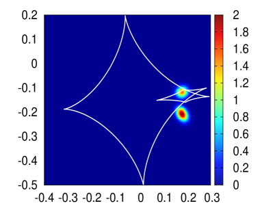
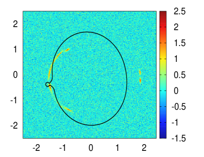
To investigate the effect of modeling a subhalo with an incorrect density profile, we simulate a gravitational lens similar to SDP.81 (ALMA Partnership et al., 2015; Dye et al., 2015; Wong et al., 2015; Tamura et al., 2015; Hatsukade et al., 2015), wherein a detection of a $\sim 10^{9}M_{\odot}$ subhalo was recently reported (Hezaveh et al. 2016; see also Inoue et al. 2016). The smooth lens component is modeled with an isothermal ellipsoid plus external shear, whose parameters are chosen to match those inferred for SDP.81 by Rybak et al. (2015). The surface brightness profiles of the two primary structures in the reconstructed source galaxy are modeled with Gaussian profiles, and the simulated image is generated by ray-tracing plus the addition of Gaussian noise (see Figure 2). To be conservative, we choose a noise level such that the signal-to-noise ratio is approximately equal to 2 over the extent of the images. In addition to adding Gaussian noise, we convolve the image with a Gaussian point spread function with dispersion 0.01 arcseconds (and thus a FWHM of $\approx$ 23 milliarcseconds, comparable to ALMA’s long-baseline resolution) along both the $x$ and $y$ directions. Our aim is not to perfectly simulate SDP.81, but rather to demonstrate the systematics of subhalo modelling in the context of a realistic gravitational lens. In particular, the correlated pixel noise arising from interferometry in actual ALMA data is not simulated here, since this is not the systematic we are interested in and would unnecessarily complicate the analysis.

(a) source plane

(b) image plane

Figure 2.— Simulated gravitational lens image where the source galaxy, host galaxy and external shear are similar to SDP.81 (axes are in arcseconds), and we have added a $\sim 10^{9}M_{\odot}$ subhalo centered at (-1.5,-0.37). Here, we plot the first gravitational lens simulation listed in Table 1, where the subhalo’s inner slope is isothermal ($\gamma=2$) and the subhalo’s distance to the host galaxy is equal to the Einstein radius of the lens ($r_{0}=b$). Critical curves and caustics are also plotted.

4.1. Subhalo density profile

For the subhalo, we require a projected density profile with a variable log-slope and a smooth truncation at a specified tidal radius. To accomplish this, we choose the “cuspy halo model” of Muñoz et al. (2001), whose density profile is

$$\rho=\frac{\rho_{0}r_{t}^{n}}{r^{\gamma}\left(r^{2}+r_{t}^{2}\right)^{(n-\gamma)/2}}.$$ (15)

This model has an inner slope $\gamma$ and outer slope $n$. The Pseudo-Jaffe profile corresponds to the special case $\gamma=2$, $n=4$, so that the inner slope corresponds to that of an isothermal sphere, while the outer slope achieves a smooth truncation around the tidal radius $r_{t}$. For general $\gamma,n$ values, the projected (spherically symmetric) density profile $\kappa(r)$ and deflection $\alpha(r)$ have analytic solutions in terms of the Gaussian hypergeometric function as given in Muñoz et al. (2001), which we use here. As with the Pseudo-Jaffe profile, we will fix $n=4$ for the outer slope, but will allow the inner slope to vary.

We will also consider the effect of varying the subhalo distance from the host galaxy center (while keeping the projected position of the subhalo fixed). The resulting tidal radius of the subhalo can be estimated by considering the subhalo before truncation, whose density profile can be written as $\rho=\rho_{0}(r_{t}/r)^{\gamma}$. Using the usual formula for the Jacobi radius, we find

$$r_{t}=\frac{r_{0}^{2}\kappa_{s,0}}{(3-\gamma)b}$$ (16)

where $r_{0}$ is the distance from the subhalo to the center of the host galaxy, $b$ is the Einstein radius of the host, and $\kappa_{s,0}=2\pi\rho_{0}r_{t}/\Sigma_{cr}$ (our definition differs from that of Muñoz et al. 2001 by a factor of $2\pi$).

For model fitting, we follow in the footsteps of previous work and model the subhalo explicitly with a Pseudo-Jaffe profile, which corresponds to $\gamma=2$, $n=4$ and whose projected density profile has a simple analytic form,

$$\kappa_{s}(r)=\frac{b_{s}}{2}\left[r^{-1}-\left(r^{2}+r_{t}^{2}\right)^{-\frac{1}{2}}\right].$$ (17)

The parameter $b_{s}$ is related to $\kappa_{s,0}$ by $\kappa_{s,0}=b_{s}/r_{t}$; plugging this into Eq. 16 gives $r_{t}=r_{0}\sqrt{b_{s}/b}$. Rather than vary $r_{t}$ explicitly, we will set $r_{0}=b$, which then fixes $r_{t}=\sqrt{bb_{s}}$, recovering the usual formula for the tidal radius under this assumption. Thus, our model subhalo parameters to be varied are $b_{s}$ along with the center coordinates $x_{c,s}$ and $y_{c,s}$.

4.2. Simulated gravitational lens scenarios

To investigate the effects of modeling a subhalo with an incorrect density profile, we consider four different gravitational lens simulations, which are listed and described in Table 1. In each scenario, the “actual” subhalo density profile is given by Eq. 15 and has the same projected position in the lens plane. For each simulated lens, we will follow the footsteps of previous work and fit the subhalo with a Pseudo-Jaffe model (Eq. 17), whose tidal radius is fixed by the condition that its distance to the host galaxy center $r_{0}$ is equal to the Einstein radius $b\approx$ 1.6” $\approx$ 7.4 kpc. Compared to the model subhalo, the “actual” subhalo density profile is identical in Simulation 1, has a shallower inner slope $\gamma$ in Simulations 2-3, and has a much larger distance from the host galaxy $r_{0}$=100 kpc in Simulation 4. Note that a larger $r_{0}$ also implies a significantly larger the tidal radius $r_{t}$ according to Eq. 16.

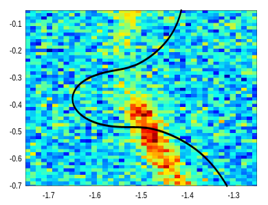
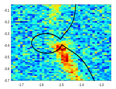
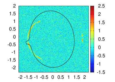
The simulated image and source planes for Simulation 1 are shown in Figure 2. In the first simulation (which is our “control” scenario since the actual subhalo profile matches the model), we choose the normalization of the density profile $\kappa_{s,0}$ so that the total subhalo mass is approximately $10^{9}M_{\odot}$. In the three remaining simulations, the normalization is chosen so that the mass within the subhalo perturbation radius $\delta\theta_{c}$ is roughly the same in each case, thus ensuring that the scale of the perturbation is not radically different in each case. Figure 3 plots the surface brightness and critical curves in each simulation. We see that indeed, the scale of the critical curve perturbation is approximately the same, although the shape of the perturbation differs: the steeper the subhalo density profile, the more the critical curve is “pinched”; likewise, the critical curve is pinched slightly more for a larger tidal radius.

For each scenario, we model the smooth lens component as a power-law ellipsoid (Tessore & Metcalf, 2015; Barkana, 1998), whose density profile can be expressed as

$$\kappa_{0}(x,y)=\frac{2-\alpha}{2}b^{\alpha}\left(qx^{2}+y^{2}/q\right)^{-\frac{\alpha}{2}}$$ (18)

where $q$ is the axis ratio. In this form, $b$ can be thought of as the average Einstein radius, since the semimajor axis of the critical curve is equal to $b/\sqrt{q}$ while the semiminor axis is equal to $b\sqrt{q}$. Eq. 18 is then rotated by an angle $\theta$, where we define the $\theta$ to be the (counterclockwise) angle between the galaxy’s semimajor axis and the $y$-axis of the observer’s coordinate system. Finally, in addition to the host galaxy, we add an external shear term which we parameterize by the shear components $\Gamma_{1}$, $\Gamma_{2}$.

	$b$	$\alpha$	$q$	$\theta$	$x_{c}$	$y_{c}$	$\Gamma_{1}$	$\Gamma_{2}$	$b_{s}$	$x_{c,s}$	$y_{c,s}$	-$\log\mathcal{E}$
Actual values	1.606	1	0.82	8.3$\degree$	-0.019	-0.154	0.0358	0.0038	—	-1.5	-0.37	—
Simulation 1	1.606	1.018	0.814	8.623$\degree$	-0.019	-0.156	0.0368	0.0026	0.0321	-1.495	-0.372	13978
Simulation 2	1.603	1.390	0.690	8.696$\degree$	-0.045	-0.160	0.0690	0.0085	0.0436	-1.492	-0.369	14004
Simulation 3	1.606	1.394	0.680	9.829$\degree$	-0.045	-0.163	0.0663	0.0047	0.0504	-1.473	-0.367	14082
Simulation 4	1.607	1.380	0.720	7.652$\degree$	-0.045	-0.157	0.0686	0.0110	0.0456	-1.503	-0.375	13989

Table 2Best-fit model parameters for each simulated lens scenario (see Table 1 for a descriptive comparison of each simulation). The top row gives the actual parameters which are the same for all four simulations, except for $b_{s}$ since the subhalo model differs for each simulation. The remaining rows give the best-fit model parameters in each case. The final column gives the logarithm of the Bayesian evidence $\mathcal{E}$ for a goodness-of-fit comparison (Suyu et al. 2006).

4.3. Lens modeling algorithm

To model our simulated lenses, we use the method of pixel-based source reconstruction, where the source is pixellated and the pixel values are inferred by linear inversion. Since this method is well-described in many papers (see e.g. Tagore & Keeton 2014, Warren & Dye 2003, Suyu et al. 2006), we do not describe it in great detail in here, but rather point out distinct features of our algorithm.

For a given set of lens parameters, we use linear 3-point interpolation for the ray-tracing to construct the lensing matrix $L$, which is well-described in Tagore & Keeton (2014). We use curvature regularization for smoothing of the source, and perform a matrix inversion to obtain the inferred source surface brightness pixel map. The reconstructed source is pixellated using an adaptive Cartesian grid (Dye & Warren, 2005), where the first-level pixels split into four smaller ones if the magnification of a source pixel is higher than $4\mu_{0}$, where $\mu_{0}$ is called the splitting threshold. This process is then repeated recursively for the higher-level pixels. For simplicity, the number of first-level source pixels is fixed to $0.3$ times the number of image pixels being fit. (We note however that more sophisticated adaptive source grids are possible; see e.g. Vegetti & Koopmans 2009 and Nightingale & Dye 2015.)

Apart from these points, we enumerate here the features that are unique in our implementation:

1) In principle, the splitting threshold can be varied and the optimal value inferred from maximizing the Bayesian evidence. In practice we find that $\mu_{0}\approx 5-6$ is typically preferred, so to save computation time we fix the splitting threshold to $\mu_{0}=5$.

2) Although our adaptive source grid is Cartesian, its borders are not fixed, but instead are redrawn each time the lens parameters are varied so that it is just large enough to include the inferred source signal. In this way, we exclude as many pixels as possible that only contain noise which could degrade the fit. In practice, we accomplish this by drawing the box so that it just barely contains all pixels for whom the surface brightness is greater than 1.3 times the pixel noise. To be conservative, we then extend the length and width of the box by 15% to make sure all the signal is being included. A side benefit of this is that computation time is saved, since typically fewer pixels are being evaluated compared to a fixed grid.

(a) Sim 1 ($\gamma$=2, $r_{t}=0.22^{\prime\prime}$)

(b) Sim 2 ($\gamma$=1.5, $r_{t}=0.24^{\prime\prime}$)

(c) Sim 3 ($\gamma$=1, $r_{t}=0.27^{\prime\prime}$)

(d) Sim 4 ($\gamma$=2, $r_{t}=2.6^{\prime\prime}$)

Figure 3.— Zoomed-in region around the subhalo in each of the simulated gravitational lenses (which are described in Table 1), with critical curves shown. Note that the subhalo perturbation radius is approximately the same in each simulation, i.e., the “size” of the critical curve perturbation is the same (by design). However, the shape of the critical curve perturbation differs dramatically: the critical curve is “pinched” more with a steeper subhalo profile, or with a larger tidal radius.

3) As is common practice, we mask regions of the image which only contain noisy pixels, so that the majority of the pixels being fit to contain the actual signal. However, there is a risk that certain solutions produce images in the masked region (i.e. outside the region being fit) that should not exist, and this may be missed. To avoid this, after inverting to find the source surface brightness distribution, we then reconstruct the lensing matrix using all of the pixels in the image, including the masked regions, and find the resulting surface brightness in each pixel. We then impose a penalty function prior, so that if the surface brightness in the masked region rises above 30% of the brightest pixel in the image, a steep penalty is imposed and this solution is discouraged.

4) In subhalo modeling studies that have used pixellated source reconstruction to date, typically an nonparametric approach (Hezaveh et al., 2016; Vegetti & Koopmans, 2009) is first used to attempt to locate where the lensing potential is being perturbed by a subhalo, before proceeding to the full parameterized subhalo model. One very important reason for doing so, rather than a parametric fit alone, is that if the mass distribution of the smooth lens component is more complicated than the chosen parametric model, spurious detections can result in an attempt to improve the fit (Vegetti et al., 2014). In this paper, since we are working with simulated data, we skip this step entirely; from a practical standpoint, this is possible thanks to an adaptive Markov Chain Monte Carlo (MCMC) algorithm called T-Walk (Christen & Fox, 2010), which is uniquely suited to efficient exploration of multimodal distributions. The T-Walk algorithm uses a Metropolis-Hastings step, but at each step, certain chains perform a “jump” over the current point in another, randomly chosen chain in an attempt to find new modes in the posterior distribution. In addition, linear coordinate transformations are performed in order to better handle parameter degeneracies. While a substantial number of chains may be required to confidently sample the parameter space, we find the T-Walk algorithm nevertheless converges much faster than a nested sampling algorithm even if there are many separate modes in the parameter space. One important benefit is that if there are multiple subhalo perturbations in the lensed image, the MCMC can find both modes even if only one subhalo is included in the model. One disadvantage of using T-Walk, however, is that it is not necessarily clear ahead of time how many chains will be needed to sample all the modes in the parameter space—for this reason along with the reasons stated above, a nonparametric analysis to identify lens perturbations in actual data is still recommended before proceeding to the MCMC.

(a) Sim 1, data

(b) Sim 1, best-fit solution

(c) Sim 3, data

(d) Sim 3, best-fit solution

Figure 4.— Pixel surface brightness data for Simulations 1 and 3, along with best-fit reconstructions and critical curves. (See Table 1 for a descriptive comparison of each simulation.) Note that in the reconstructed image plane for Simulation 3, a small additional image is present near the position of the subhalo which does not appear in the data; this is a consequence of modeling the subhalo with a steeper profile compared to the actual subhalo. Despite this, although the shape of the critical curve perturbation is different compared to the data, the scale of this perturbation $\delta\theta_{c}$ is remarkably well-reproduced.

(a) Sim 1, best-fit reconstructed source

(b) Sim 3, best-fit reconstructed source

Figure 5.— Reconstructed source plane for Simulations 1 and 3. The actual source surface brightness distribution is the same for all the simulations and shown in Figure 2(a). Note that source pixels are recursively split into 4 smaller subpixels in regions of high magnification. Despite the differences in each simulated lens image and reconstruction, the source structure is well-reproduced in each case, although the position and scale of the source pixels vary somewhat between the different simulations.

Figure 6.— Posterior probability distributions in the parameters for Simulation 3, where the subhalo has an inner log-slope -1 (see Table 1 for description). To reduce clutter, we have not shown the posteriors for the position of the host galaxy ($x_{c}$,$y_{c}$) or the regularization parameter, which are very well-constrained. Note that the log-slope of the host galaxy $\alpha$ is biased high, which attempts to mitigate the overly “sharp” perturbation created by the steeper density profile of the subhalo (inner log-slope -2) in the model.

	$m_{T}/10^{9}M_{\odot}$	$m_{T,fit}/10^{9}M_{\odot}$	$\Delta m_{T}/m_{T}$	$\delta\theta_{c}$ (kpc)	$\tilde{m}_{sub}/10^{9}M_{\odot}$	$\tilde{m}_{sub,fit}/10^{9}M_{\odot}$	$\Delta\tilde{m}_{sub}/\tilde{m}_{sub}$
Simulation 1	1.027	1.058	3.02%	0.679	0.473	0.476	0.60%
Simulation 2	1.504	1.674	11.3%	0.716	0.494	0.518	4.87%
Simulation 3	2.341	2.100	10.3%	0.809	0.592	0.662	11.7%
Simulation 4	8.698	1.794	79.4%	0.744	0.519	0.556	7.12%

Table 3Comparison of subhalo mass estimators for the actual vs. best-fit values in each simulated gravitational lens (see Table 1 for a descriptive comparison of each simulation). $m_{T}$ refers to the total subhalo mass, while the effective subhalo mass $\tilde{m}_{sub}\equiv m_{sub}(\delta\theta_{c})/\alpha$ is the projected subhalo mass enclosed within the subhalo perturbation radius $\delta\theta_{c}$ (which we list in parsecs in the middle column). Note that for Simulation 4, where the subhalo has a substantially larger tidal radius, the inferred total subhalo mass $m_{T}$ is off by $\sim 80$% while the effective subhalo lensing mass $\tilde{m}_{sub}$ is recovered very well by comparison.

(a) Simulation 1 ($\delta\theta_{c}\approx 0.149$”)

(b) Simulation 2 ($\delta\theta_{c}\approx 0.155$”)

(c) Simulation 3 ($\delta\theta_{c}\approx 0.175$”)

(d) Simulation 4 ($\delta\theta_{c}\approx 0.161$”)

Figure 7.— Best-fit mass profile of the subhalo compared to the true profile in each simulated lens, scaled by $1/\alpha\Sigma_{cr}$ (where $\alpha$ is the log-slope of the host galaxy’s density profile). For a descriptive comparison of each simulation, see Table 1. The vertical dashed line denotes the subhalo perturbation radius $\delta\theta_{c}$, which is the radius where the critical curve is maximally perturbed by the subhalo in the best-fit model; the best-fit $\delta\theta_{c}$ is given below each plot for comparison. In all cases except for Simulation 1, the total mass of the best-fit model is biased due to the mismatched density profile; nevertheless the mass enclosed within $\delta\theta_{c}$ is well-recovered, provided it is scaled by $1/\alpha$.

5. Results

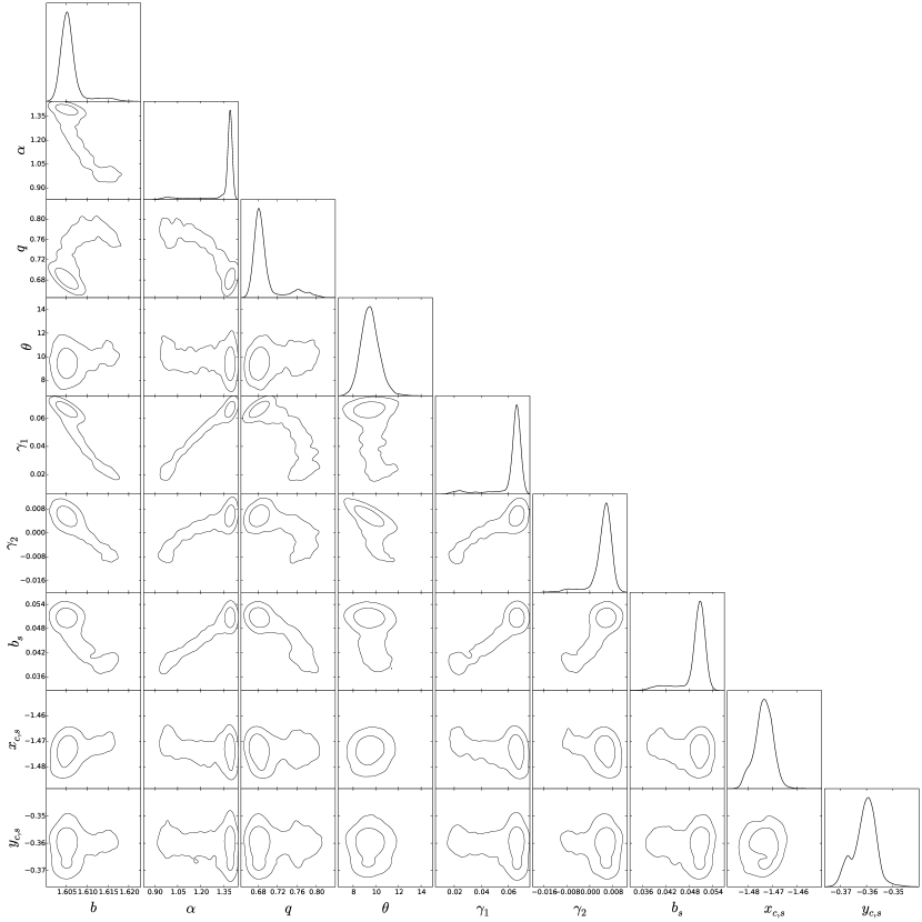
After running the T-Walk MCMC algorithm to explore the parameter space, posteriors are generated in each parameter; we plot the resulting joint posteriors for Simulation 3 in Figure 6. Finding the correct parameter space for the subhalo required a substantial number of chains (up to 96 chains). In the process, the chains found several false modes in parameter space with the subhalo located incorrectly, that partially mimicked the effect of the subhalo. Typically these false modes involved at least one extra source structure; for example, in one mode, one of the actual source structures was split into two, each of which were highly magnified. These kinds of modes involved a greater number of subpixels and/or greater regularization, and hence were disfavored by the Bayesian evidence compared to the “correct” mode. This highlights a major advantage of using the Bayesian evidence (beyond just setting the optimal regularization, which is discussed extensively in Suyu et al. 2006) rather than simply the likelihood.

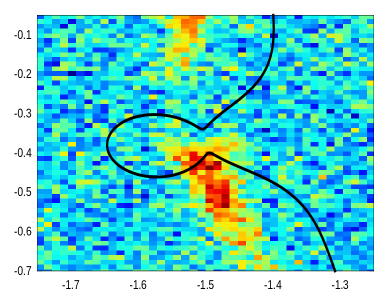
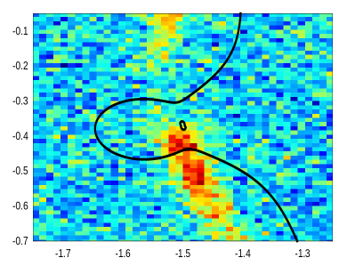
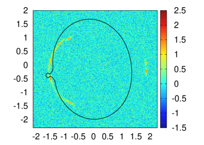
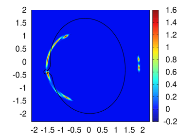
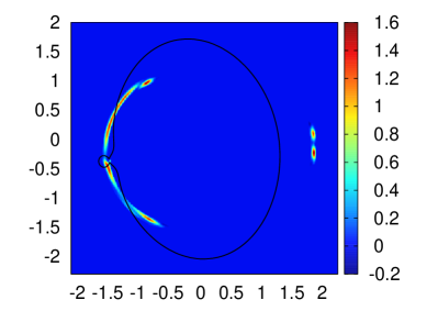
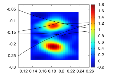
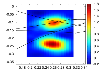
The resulting best-fit parameters in each case are shown in Table 2. For reference, we plot the reconstructed image and source planes for Simulations 1 and 3 in Figures 4 and 5 respectively. As expected, the model parameters in Simulation 1 are well-recovered, since the subhalo density profile is the same as in the model. In the other simulations, the position of the subhalo is fairly well-recovered, but some of the host halo parameters are biased in an attempt to make up for the fact that the subhalo in the model does not perfectly reproduce the observed perturbation. Most prominently, the model prefers the log-slope of the host galaxy’s profile $\alpha$ to be greater than 1; in fact, the best-fit values of $\alpha$ were close to our upper prior limit of 1.4. We believe this effect is a consequence of the shallower projected density profile in the actual subhalo in each simulation. In these cases, as Figure 3 shows, the subhalo perturbation is less “sharp” and does not pinch the critical curve as dramatically compared to the Pseudo-Jaffe subhalo; as a result, the magnification is lower in the vicinity of the subhalo. One consequence of this is that a small additional image is evident just to the right of the subhalo in Simulation 1 (Figures 4(a), 4(b)), whereas for Simulations 2-3 which have shallower profiles, these additional images are not evident (see Figure 4(c) for Simulation 3). Nevertheless, in the reconstructed solution, a small additional image does appear (Figure 4(d)), which is inevitable because we are modeling with a Pseudo-Jaffe subhalo. It seems that having a steeper density profile for the host galaxy mitigates this effect by reducing the magnification and hence the size of the additional image produced by the Pseudo-Jaffe subhalo, and hence a steeper log-slope $\alpha$ is preferred. However, this does not mean that $\alpha=1$ was excluded in all cases; for example, in Simulation 3, the posterior extends all the way down to $\alpha\approx 1$ (see Fig. 6), although the fit is not as good there.

5.1. How biased is the inferred mass of the subhalo?

To investigate the bias in the inferred subhalo mass in each scenario, in Table 3 we show the “true” total subhalo mass and the best-fit subhalo mass for each scenario. As expected, the total subhalo mass is well-recovered in Simulation 1, since the subhalo density profile matches that of the model. In Simulations 2 and 3 where the slope of the density profile differs but the subhalo distance matches the model ($r_{0}=b$), the error is still fairly small, roughly 11% in each case. This is a fortunate consequence of the fact that the scale of subhalo lensing perturbation is naturally similar to the tidal radius under this assumption, as discussed in Section 2. However, the situation is very different if the tidal radius differs significantly from the model, as is evident in the Simulation 4 results: here, the actual subhalo mass is nearly five times larger than the inferred mass, with an error of nearly 80%. The reason is clear: in this case the subhalo’s tidal radius is approximately 2.6 arcseconds, compared to 0.27 arcseconds in the best-fit model. Thus, the subhalo’s density profile extends much further out compared to the model, and beyond the critical curve perturbation radius $\delta\theta_{c}$, this extra mass can be “hidden” by adjusting the smooth lens component. This high systematic error in the total subhalo mass has also been pointed out by Vegetti et al. (2012) and Vegetti & Vogelsberger (2014) (indeed they estimate this error by considering different projected distances to the lens plane, under the assumption that the subhalo number density traces the dark matter profile of the host galaxy).

It has been suggested in Vegetti & Vogelsberger (2014) that the mass enclosed within the subhalo’s Einstein radius is robust to changes in the density profile, so we also test this idea on our simulated lenses. With the exception of Simulation 1 (where the subhalo’s density profile and tidal radius are correctly modeled), we find that at the subhalo’s Einstein radius $b_{s}$ in the best-fit model (which is in the range 0.04-0.05”; see Table 2), the enclosed subhalo mass is significantly overestimated. In the most extreme case, Simulation 3, the best-fit subhalo mass enclosed within its Einstein radius is $\sim$ 3.5 times larger than the actual mass, an error of 250%. It is also worth noting that the Einstein radius of the actual subhalo can also be dramatically different from the model if the slope of the density profile differs enough; in Simulation 3, the true Einstein radius of the subhalo is $7.3\times 10^{-4}$ arcseconds, much smaller than the Einstein radius of the best-fit model subhalo. Thus, we conclude that the Einstein radius of the subhalo itself plays no special role and the inferred mass within this radius is not robust to changes in the density profile.

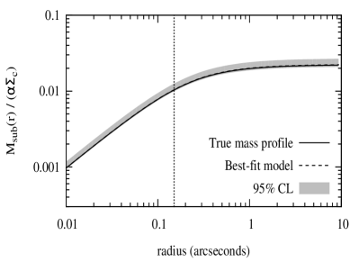
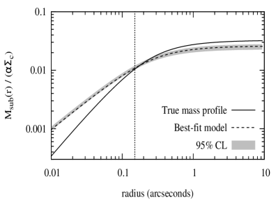
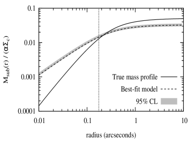
5.2. Robustness of the effective subhalo lensing mass

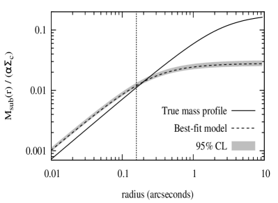
Having established that the bias in the inferred subhalo mass can be significant, we now investigate whether the effective subhalo lensing mass $\tilde{m}_{sub}\equiv m_{sub}(\delta\theta_{c})/\alpha$ (defined in Section 2) can indeed be considered a robust mass estimator. In Figure 7 we plot the subhalo mass profile of the best-fit model in each case (dashed line) divided by the log-slope $\alpha$ of the host galaxy, compared to the actual subhalo mass profile (solid line; recall that $\alpha=1$ for the actual model in each case). The shaded region denotes the 95% confidence interval, which is obtained by calculating a derived posterior probability in the subhalo mass enclosed within each radius. Simulation recovers the mass profile very well, as expected; for the remaining cases, the mass enclosed within $\delta\theta_{c}$ (denoted by the dotted vertical line) divided by $\alpha$ is indeed quite close to the actual subhalo mass even though the mass elsewhere is different. In Table 3 the values for $\tilde{m}_{sub}$ are tabulated along with the error. In Simulation 4, the error in this quantity is roughly 8%, a vast improvement compared to the discrepancy in the total subhalo mass. With the exception of the shallowest density profile $\gamma=1$ (Simulation 3), the error in $\tilde{m}_{sub}$ is significantly smaller than the error in the total subhalo mass.

Further evidence for the invariance of the effective subhalo mass $\tilde{m}_{sub}$ can be seen in the posteriors themselves. In the parameter region where the data are well-fit, if $m_{sub}(\delta\theta_{c})/\alpha$ is invariant then it follows that $b_{s}/\alpha$ must also be approximately invariant. Indeed, this can be seen in the approximate formula Eq. 11: to highest order, $\delta\theta_{c}$ will remain the same if the ratio $b_{s}/\alpha$ is fixed. Thus we expect a linear degeneracy between the parameters $b_{s}$ and $\alpha$, which is shown beautifully in the joint posterior in these parameters in Figure 6. For the best-fit solution, we have $b_{s}\approx 0.05$, $\alpha\approx 1.4$, and thus the ratio $b_{s}/\alpha\approx 0.036$. If we pick a different point, for example where $\alpha=1.2$, then to maintain this ratio we must therefore have $b_{s}\approx 0.036\times 1.2\approx 0.043$, and indeed this value falls within the allowed parameter region in the figure. The relationship is not satisfied quite as well for $\alpha=1$, where the posterior lies slightly above the expected value $b_{s}\approx 0.036$; however, in this region the subhalo position has drifted further away from the critical curve, which can be seen in the joint $\alpha$-$x_{c,s}$ posterior at $\alpha=1$. Since the subhalo position has shifted, the effective subhalo lensing mass will change, and in order to produce the same critical curve perturbation $b_{s}$ needs to be slightly larger, as the posterior shows. Nevertheless, in the neighborhood of the best-fit region it is clear that the $\alpha$-$b_{s}$ degeneracy is fully consistent with the invariance of the effective subhalo lensing mass $\tilde{m}_{sub}$.

5.3. Sources of bias in the effective subhalo lensing mass

Although Figure 7 shows that the effective subhalo lensing mass $\tilde{m}_{sub}$ is fairly robust, it is also biased a little bit high in each case. Why is this? There are two reasons. First, although $\delta\theta_{c}$ in the best-fit model is close to the actual value in each case, it is not exactly the same—it differs, either because the critical curve perturbation itself is larger or the subhalo is slightly farther from the unperturbed critical curve compared to the actual subhalo. This is most evident in Simulation 3, where the best-fit subhalo position is offset by 0.03 arcseconds to the right compared to the true position; this partly accounts for the larger $\delta\theta_{c}$ in the best-fit model for Simulation 3, since the subhalo is further from the critical curve. This shifting of the subhalo away from the actual position of the critical curve is a compromise to avoid an overly “sharp” pinching of the critical curve (and corresponding high magnification at the position of the subhalo) that results from the steeper density profile in the model subhalo. Likewise, the size of the critical curve perturbation itself may differ slightly as a compromise in order to better fit the perturbed surface brightness at different radii; given that the surface brightness variations will differ from lens to lens, the bias due to this is very difficult to quantify in general.

The second reason for the bias is due to differences in the smooth lens component. As is evident in Table 2, having a different log-slope $\alpha$ is not the only difference in the host galaxy parameters compared to their actual values. There is also a slightly different external shear $\Gamma_{ext}$ (specifically, the $x$-component $\Gamma_{1}$) and axis ratio $q$, and additionally the host galaxy is shifted significantly to the left. All of these change the left-hand side of Eq. 1, and hence the subhalo mass enclosed within $\delta\theta_{c}$ is not strictly invariant. Part of this can be specifically accounted for: in Appendix B it is shown that, assuming the subhalo position is well-reproduced, the invariant quantity is actually $m_{sub}(\delta\theta_{c})/\alpha\eta=\tilde{m}_{sub}/\eta$ (Eq. B15), where the parameter $\eta$ is determined by the external shear $\Gamma_{ext}$ (Eq. B10). Thus, we should have $\tilde{m}_{sub,fit}\approx m_{sub,true}\frac{\eta_{fit}}{\eta_{true}}$. In this case the direction of the subhalo $\phi$ and the direction of the external shear perturber $\phi_{p}$ differ by 90 degrees, so we have $\eta\approx 1+\Gamma_{ext}\approx 1+\Gamma_{1}$. Thus, using the best-fit values from Table 2, we have $\eta_{true}\approx 1.036$, while $\eta_{fit}\approx 1.07$ for Simulations 2-4. Thus, $\tilde{m}_{sub}$ is inflated by a factor of $1.07/1.036\approx 1.03$, or about 3% in each case. While this doesn’t account for all of the error in $\tilde{m}_{sub}$, we can see in the final column of Table 3 that it accounts for roughly half the error in Simulations 2 and 4 (though only a quarter of the error in Simulation 3; much of the remaining error is likely due to the offset position of the subhalo). Unfortunately, the factor $\eta$ doesn’t allow us to improve our mass estimator, because there is no way to know the true external shear (and hence $\eta_{true}$), but it at least allows us to quantify the error due to this effect in simulated cases.

Even if it were possible to have prior knowledge of the true parameters of the smooth lens component, fixing these to their correct values does not improve the fit; indeed, it makes it worse. The more freedom the smooth lens component has to partially mimic the effect of the subhalo beyond $\delta\theta_{c}$, the better the subhalo model will be able to reproduce the subhalo perturbation radius and hence, the (scaled) mass within $\delta\theta_{c}$. Thus, having sufficient freedom to vary the smooth lens component is essential to achieving a good fit, even if a small amount of bias inevitably results in these parameters as a result of the mismatched subhalo density profile. In fact, it may be beneficial to include additional components to the smooth lens model beyond what we have done here—in particular, higher-order multipole moments might allow for a better fit in the region of the subhalo, but we have not explored this option in this work.

(a) variable subhalo mass

(b) variable subhalo position

Figure 8.— Fractional error in effective lensing mass $\tilde{m}_{sub}$ from the best-fit subhalo (solid line), for different values of the “true” subhalo parameters for a subhalo 100 kpc from the lens plane (as in Simulation 4). In (a) the subhalo mass is varied, while in (b) we vary the subhalo’s projected separation from the host galaxy center; each time the parameter is varied, the evidence is minimized to find the best-fit model. To judge the quality of the fit, we compare the Bayesian evidence obtained from the best-fit model with vs. without a subhalo included in the model (dotted line); this is quantified by $\Delta\log\mathcal{E}=\log\mathcal{E}_{sub}-\log\mathcal{E}_{nosub}$. The vertical dotted line in (b) denotes the position of the critical curve along the direction of the subhalo. Note that in cases where the effective lensing mass is inaccurate by more than $\sim$ 20%, the Bayesian evidence does not prefer including a subhalo to high significance (i.e., $\Delta\log\mathcal{E}$ is either negative or is not significantly greater than the noise).

6. Range of validity of the effective subhalo lensing mass

Thus far we have only tested our subhalo mass estimator $\tilde{m}_{sub}$ in one example lens scenario, in which we have varied only the subhalo density profile and/or tidal radius. This begs the question, how accurate is $\tilde{m}_{sub}$ for subhalos of different masses, or at different positions relative to the images or critical curve? In this section we will consider different scenarios where these subhalo parameters are varied. For simplicity, we will consider only a subhalo at 100 kpc from the lens plane (as in Simulation 4; see Table 1), which has a considerably larger tidal radius compared to the subhalo model being used in the analysis. It would be computationally very expensive to perform an MCMC over a large number of scenarios, so here we take a different approach, by minimizing the Bayesian evidence for each scenario using our fiducial subhalo model.

The procedure is as follows. We start with the “true” subhalo parameters identical to Simulation 4, and minimize the Bayesian evidence to find the best-fit model (using our solution in Table 2 as the initial guess parameters). We then vary one of the “true” subhalo parameters by a small amount, generate a new data image (with different random noise added to the image each time), and minimize the Bayesian evidence again, using our previous best-fit model as the initial guess parameters; then we repeat the cycle. In this way, we generate a “chain” of solutions, and for each solution we calculate the subhalo perturbation radius numerically and hence, the effective lensing mass $\tilde{m}_{sub}$. To test the quality of the fit, we also fit a model that does not include a subhalo and compare the Bayesian evidence of the best-fit model with vs. without a subhalo.

The results are shown in Figure 8, where in each figure we plot the fractional error in $\tilde{m}_{sub}$ (solid line, left axis) and the difference in the Bayesian Evidence (dashed line, right axis). In Figure 8(a), we have varied the mass normalization of the subhalo (i.e. the parameter $b_{s}$) and plot with respect to the total subhalo mass. In Figure 8(b), we varied the subhalo’s projected distance from the host galaxy center, keeping the subhalo’s position angle with respect to the $x$-axis fixed; the dotted vertical line denotes the position of the critical curve along the direction of the subhalo (for comparison, the image being perturbed by the subhalo is roughly at $\sim 1.5$ arcseconds). In each case, note that in the regime where the error in $\tilde{m}_{sub}$ is less than $\sim$20%, the difference in Bayesian evidence $\Delta\log\mathcal{E}$ is positive and significantly greater than the fluctuations generated by the random noise, indicating that the subhalo model is favored in these cases. Conversely, when $\tilde{m}_{sub}$ rises well above 20%, $\Delta\log\mathcal{E}$ is either negative or is not significantly greater than the fluctuations, indicating that the subhalo detection is not favored in these cases. This gives us confidence that the effective subhalo lensing mass is relatively unbiased if the subhalo model is favored by the Bayesian evidence.

Note that in Figure 8(a), as the true subhalo mass rises above $\sim 5\times 10^{9}M_{\odot}$, the effective lensing mass $\tilde{m}_{sub}$ becomes gradually more inaccurate, even though the subhalo model is strongly favored. This is because the fit becomes gradually poorer for very strong subhalo perturbations, since the lensing effect of the true subhalo is more pronounced and more difficult to reproduce with the assumed subhalo model (which has a much smaller tidal radius, in this simulation). Hence the effective lensing mass becomes more biased for large subhalo masses.

Although Figure 8(a) suggests that only subhalos with total mass greater than $\sim 3\times 10^{9}M_{\odot}$ can be detected with confidence with an ALMA-like resolution ($\sim 0.01$ arcseconds), there are ways to lower this detection threshold. First, smaller mass subhalos should be detectable if both the subhalo and the image being perturbed are closer to the critical curve. This effect is enhanced if the lens itself is more symmetrical, resulting in highly magnified arcs where subhalo perturbations are amplified. In addition, the signal-to-noise ratio in our simulations is $\approx 2$, which is relatively low; for long exposures where the signal-to-noise is higher, detection of smaller subhalo perturbations becomes easier. Thus, detection of lower mass subhalos is still possible even with the current resolution limit.

7. Discussion

7.1. Can the subhalo position be well-fit in realistic scenarios?

While we have demonstrated in Section 5 that our subhalo mass estimator $\tilde{m}_{sub}$ can be determined robustly, we have seen in Section 6 that this condition depends on achieving a good fit, such that the subhalo model is favored by the Bayesian evidence. In particular, the fit must be good enough so that the inferred position of the subhalo is reasonably accurate (such that the error in the subhalo’s position is small compared to the subhalo’s distance to the critical curve, $\delta\theta_{c}$). One can see from Table 2 that this is true for each of the simulations analyzed in this paper. However, in Simulation 3 the subhalo’s position has the greatest error, with the best-fit position shifted by nearly 0.03 arcseconds further from the critical curve. This is a consequence of the true subhalo’s density profile having a much shallower slope ($\rho\sim r^{-1}$) compared to the model subhalo ($\rho\sim r^{-2}$). If the model subhalo is too close to the critical curve, it “pinches” the critical curve too much (recall the difference in perturbation shape from Figure 3), resulting in a perturbation that cannot fit the data well, so a compromise is reached where the best-fit subhalo is a bit further out. Indeed, by comparing the Bayesian evidence $\mathcal{E}$ in the last column of Table 2, one sees that of the four simulations we modeled, Simulation 3 gave the poorest fit, and also gave the greatest error in the effective lensing mass (Table 3).

Is it possible to have a realistic scenario where the density profile and tidal radius of the subhalo differ so dramatically from the model that a good fit cannot be achieved at all? While we cannot say for sure yet, it is conceivable that a typical NFW subhalo may fall in this category. In this paper we varied the suhalo’s log-slope and tidal radius separately, to isolate each effect. However, if the true subhalo has an NFW profile, it can be expected to exhibit a combination of these two effects—that is, a shallow inner log-slope of -1, plus a larger tidal radius since we expect $r_{0}>b$. In this case, the discrepancy in the inferred total subhalo mass will be even more profound than it was for Simulation 4, since the density profile would not fall off as quickly beyond $\delta\theta_{c}$ and more mass would lie outside the subhalo perturbation radius. More worringly, the perturbation of the neighboring images differs so much compared to the Pseudo-Jaffe model that it is questionable whether such a scenario could even be well-fit by a Pseudo-Jaffe subhalo at all. If so, the implication would be that the substructures detected thus far in gravitational lenses cannot correspond to NFW subhalos with realistic tidal radii. However, as we have not attempted to fit simulated data with an NFW subhalo in this paper, this remains an open question at present.

7.2. Implications of the bias in the inferred density profile of the host galaxy

The effect we have seen on the log-slope of the host galaxy $\alpha$ is rather striking, and it is tempting to interpret an $\alpha>1$ result from an actual dataset as evidence that the subhalo density profile is indeed shallower than isothermal or that the tidal radius is underestimated. In Vegetti et al. (2010), the inferred log-slope $\alpha\approx 1.2$, which could be consistent with the scenarios discussed here. On the other hand, in Vegetti (2012) they infer $\alpha\approx 1.05$, while for SDP.81, Hezaveh et al. (2016) find $\alpha\approx 1.06$; in both cases, the slope of the host galaxy’s profile is just barely consistent with isothermal. If taken at face value, this might suggest that the subhalo density profile cannot be much shallower than isothermal. However, we must be cautious when interpreting these results. It may be the case that the host galaxy’s density profile may have a log-slope somewhat less than 1, in which case these results could still be consistent with a shallower subhalo profile. Indeed, Schneider & Sluse (2013) show that the log-slope of the host galaxy in the vicinity of the images can be expected to be biased due to the mass-sheet degeneracy if the galaxy’s profile differs from a strict power-law at other radii. Furthermore, even if the true $\alpha$ is very close to 1 in these cases, the parameter-space solution may not necessarily be unique. As is clear in Figure 6, $\alpha=1$ may still be a viable region of parameter space; if $\alpha$ is fixed to 1, the subhalo may still be found in that parameter space even if the fit is poorer compared to having a steeper $\alpha$. Thus, it is possible that in these cases, a mode with higher $\alpha$ might be found by a more complete multimodal sampling of the parameter space, e.g. using the T-Walk algorithm, and would produce an even better fit.

Ultimately, to minimize the bias in both the inferred subhalo properties and the host galaxy parameters, the ideal approach is to vary both the subhalo’s tidal radius $r_{t}$ and inner log-slope $\gamma$ as free parameters. However, while it remains to be seen how well a subhalo’s density profile can be constrained, e.g. in high-resolution ALMA images of submillimeter gravitational lenses, it seems likely that the tidal radius will be prior-dominated given that the subhalo pertubation beyond $\delta\theta_{c}$ can be mimicked by perturbing the smooth lens component, and hence the exact tidal radius will be difficult to constrain. Therefore, given the difficulty in constraining these parameters (together with the added computational expense of varying them), we argue the effective subhalo lensing mass $m_{sub}(\delta\theta_{c})/\alpha$ is a very useful quantity given that it is largely robust to changes in the subhalo’s density profile and tidal radius. Given several subhalo detections, one could use these mass measurements to test whether they are consistent with the expected mass function from $\Lambda$CDM, or whether an alternate dark matter scenario (e.g., warm dark matter) would provide a better fit.

7.3. Procedure for calculating the subhalo perturbation radius

In this section, we provide a summary of procedures for calculating the subhalo perturbation radius $\delta\theta_{c}$ for a given lens model, at different levels of approximation.

If the model subhalo is isothermal/Pseudo-Jaffe and one is content with approximating $\delta\theta_{c}$ to 20-30% accuracy, we recommend using Eq. 11 due to its relative ease of use. Despite the approximation, the subhalo mass within this radius is still quite robust (and in fact works slightly better than the exact values in our Simulations 2-4). For lens modelers who wish to calculate $\delta\theta_{c}$ to better accuracy, the more rigorous Eq. B23 can be used, or Eq. 1 can be solved numerically.

To solve for $\delta\theta_{c}$ numerically using Eq. 1 (which works regardless of the model being used for the subhalo profile), one could adopt the following method. Calculate the direction $\phi_{\Gamma}$ of the unperturbed shear $\boldsymbol{\Gamma_{tot}}$ at the position of the subhalo. The solution to Eq. 1 will lie somewhere along the line perpendicular to this direction, i.e. along $\phi_{r}=\phi_{\Gamma}+90\degree$, because along this line the subhalo’s shear aligns with the shear of the unperturbed lens model. In this way, Eq. 1 is reduced to an equation in $r$, which can be found with a root-finding algorithm.

To get a sense of the relative accuracy of these different methods, in Table 4 in Appendix B we list a comparison of the $\delta\theta_{c}$ value calculated numerically using this procedure, and the values calculated using both Eq. 11 and the more exact Eq. B23 for the four simulations considered in this paper.

8. Conclusions

In this article, we have investigated the bias that results from modeling a dark matter subhalo in a strong gravitational lens with an incorrect density profile. We have derived formulas for the radius of the critical curve perturbation generated by subhalos (see Section 7.3 for a summary), and have shown this scale to be approximately independent of the mass distribution of the subhalo within that radius. We demonstrated the usefulness of this scale by modeling a subhalo in a gravitational lens which has a different log-slope of the density profile, and different tidal radius, compared to the model. Our key results are encapsulated in Figure 7 and Table 3.

We have found that the estimated total masses of subhalos detected in strong gravitational lens systems may be significantly biased because of our ignorance about the density profile (tidal radius and inner log-slope) of the perturbing subhalo. The most severe error, due to the unknown tidal radius, arises from our ignorance of the subhalo’s projected distance to the lens plane (this is also pointed out by Vegetti et al. 2014). However, regardless of this ignorance, we show that the effective lensing mass of the perturber, $m_{sub}/\alpha$, can be inferred accurately. The mass $m_{sub}$ is computed within a radius $\delta\theta_{c}$, defined by the perturbation of the critical curve in the vicinity of the subhalo, while $\alpha$ is the log-slope of the density profile of the host.

While we have focused on subhalos in this paper, we note that our mass estimator is equally applicable to perturbers along the line-of-sight to the lens, unassociated with the primary lens galaxy. In our notation this corresponds to the limit $r_{0}\rightarrow\infty$, where $r_{0}$ is the perturber’s distance from the lens galaxy center.

The effective lensing mass should allow for a more robust comparison to simulations and inference of the subhalo mass function from dark matter substructure detections. Whether we can go beyond this effective lensing mass and gain information about the density profile of a perturber from its effects on highly magnified images is an open question that has great relevance for the nature of dark matter.

Appendix A Appendix A: Equation for critical curve perturbations by subhalos

In this section we derive the general equation for the size of the perturbation to a critical curve generated by a subhalo.

Suppose we have a gravitational lens with a host galaxy whose density profile is denoted by $\kappa_{0}$, an external shear $\Gamma_{ext}$, and subhalo denoted by $\kappa_{s}$. To find the formula for the inverse magnification at a given position, we adopt a coordinate system where the combined shear of the host galaxy and the external shear is diagonalized. In this coordinate system, the Jacobian becomes

$$\frac{\partial{\boldsymbol{\beta}}}{\partial\boldsymbol{\theta}}=\left(\begin{array}[]{cc}1-(\kappa_{0}+\kappa_{s})-(\Gamma_{tot}-\Gamma_{s}\cos 2\phi_{s})&\Gamma_{s}\sin 2\phi_{s}\\ \Gamma_{s}\sin 2\phi_{s}&1-(\kappa_{0}+\kappa_{s})+(\Gamma_{tot}-\Gamma_{s}\cos 2\phi_{s})\end{array}\right)$$ (A1)

where $\phi_{s}$ gives the direction of the subhalo relative to the direction of the total unperturbed shear, $\boldsymbol{\Gamma_{tot}}=\boldsymbol{\Gamma_{0}}+\boldsymbol{\Gamma_{ext}}$. (Note, $\phi_{s}$ is not the shear direction of the subhalo, but rather points toward the subhalo itself. In this formula, the subhalo is assumed to be axisymmetric, so the subhalo’s shear is perpendicular to the direction of the subhalo—this accounts for the minus sign in front of $\Gamma_{s}$.) The inverse magnification is then the determinant of the Jacobian, which can be written as

$$\mu^{-1}=(\lambda_{-}-\kappa_{s}+\Gamma_{s}\cos 2\phi_{s})(\lambda_{+}-\kappa_{s}-\Gamma_{s}\cos 2\phi_{s})-\Gamma_{s}^{2}\sin^{2}2\phi_{s}$$ (A2)

where the $\lambda_{\pm}$ are the eigenvalues of the magnification of the unperturbed model,

$$\lambda_{\pm}=1-\kappa_{0}\pm\Gamma_{tot}.$$ (A3)

The set of points on the lens plane for which $\lambda_{-}=0$ corresponds to the tangential critical curve, while $\lambda_{+}=0$ corresponds to the radial critical curve. Radial critical curves do not exist if the host galaxy is isothermal, and since their effects are difficult to observe in any case, we will therefore focus on perturbations to the tangential critical curve.

After some algebraic manipulation, this can be cast into the following equation:

$$\mu^{-1}=\mu_{0}^{-1}+\mu_{s}^{-1}-1+2\kappa_{0}\kappa_{s}+2\Gamma_{tot}\Gamma_{s}\cos 2\phi_{s}$$ (A4)

Inside the tangential critical curve, the inverse magnification $\mu^{-1}$ is negative. In the case of an axisymmetric host galaxy with no external shear present, we define the direction of maximum warping of the critical curve to be the direction along which the critical curve is pushed furthest away from the subhalo, compared to its position without the subhalo present. This will be the direction for which the inverse magnification $\mu^{-1}$ is decreased the most (or rather, made more negative). According to Eq. A4, this occurs when $\phi_{s}=90\degree$, the direction along which the shear of the subhalo aligns with that of the host galaxy.

If the host galaxy is axisymmetric, its shear is parallel to the tangential critical curve, and thus $\phi_{s}=90\degree$ would be along the radial direction. For a non-axisymmetric host galaxy with external shear, the “direction of maximum warping” is a bit more ambiguous, because the comparison depends on how the critical curve is parameterized with and without the subhalo. Since the ambiguity only arises for highly asymmetric lenses and we are mainly interested in the overall scale of the perturbation, we choose the simplest approach and define $\phi_{s}=90\degree$ to be the direction of maximal warping in general.

If we return to Eq. A2 and set $\phi_{s}=90\degree$ and $\mu^{-1}=0$ to find the location of the tangential critical curve, we find

$$\lambda_{-}(\boldsymbol{\theta})=\kappa_{s}+\Gamma_{s}.$$ (A5)

Although there is also a radial critical curve solution, we are focusing only on the tangential critical curve solution involving $\lambda_{-}$. Using the fact that for an axisymmetric lens we have $\Gamma=\bar{\kappa}-\kappa$, we can rewrite the equation as follows,

$$1-\kappa_{0}(\boldsymbol{\theta_{s}}+\boldsymbol{r})-\Gamma_{tot}(\boldsymbol{\theta_{s}}+\boldsymbol{r})=\bar{\kappa}_{s}(r)$$ (A6)

where $\boldsymbol{r}=\boldsymbol{\theta}-\boldsymbol{\theta_{s}}$, and $\boldsymbol{\theta_{s}}$ is the position of the subhalo. Once the direction of $\boldsymbol{r}$ is fixed by the $\phi_{s}=90\degree$ requirement, this equation can be solved for $r$ to find the radius of maximum deformation of the critical curve. From the formula it is evident that the solution, which we call the “subhalo perturbation radius” $\delta\theta_{c}$, only depends on the mass of the subhalo enclosed within the radius $\delta\theta_{c}$ (and hence, the average kappa enclosed); it does not depend on how that mass is distributed within this radius.

Appendix B Appendix B: General solution for the subhalo perturbation radius and effective lensing mass

B.1. B1. General analytic equation for the subhalo perturbation radius

Here we will obtain a more rigorous result for the subhalo perturbation radius, in the case where the subhalo is not exactly on a critical curve and both ellipticity and external shear are present. Suppose the subhalo is located at a radius $\theta_{s}$ (not necessarily on the critical curve) and angle $\phi$ with respect to the $x$-axis, and the host galaxy has an axis ratio $q$ and major axis oriented at an angle $\phi_{0}$ with respect to the $x$-axis. Suppose also that there is an external shear $\Gamma_{ext}$ created by a distant perturbing mass whose direction is denoted by angle $\phi_{p}$.

The projected density profile of the host galaxy is modeled as a power-law ellipsoid. In a coordinate system ($x^{\prime},y^{\prime}$) where the major axis of the lens coincides with the $x^{\prime}$-axis, we write the profile as follows, using the notation $\boldsymbol{\theta^{\prime}}=(x^{\prime},y^{\prime})$:

$$\kappa_{0}(\boldsymbol{\theta}^{\prime})=\frac{2-\alpha}{2}b^{\alpha}\left(qx^{\prime 2}+y^{\prime 2}/q\right)^{-\frac{\alpha}{2}}$$ (B1)

In this formulation, the normalization parameter $b$ can be thought of as the average Einstein radius, while the semimajor axis of the critical curve is $b/\sqrt{q}$. Another common choice is to make the semimajor axis of the critical curve the normalization parameter (call it $b^{\prime}$), in which case one should substitute $b^{\prime}=b/\sqrt{q}$ in the following formulas. In any event, in the actual coordinate system of the lens plane ($x,y$), we calculate $\kappa_{0}(\boldsymbol{\theta})$ by rotating these coordinates by the angle $\phi_{0}$; in other words, by first calculating $\theta_{i}^{\prime}=\mathcal{R}_{ij}\theta_{j}$ where $\mathcal{R}_{ij}$ is the corresponding rotation matrix, and inserting into Eq. B1.

We can write this in terms of polar coordinates in the lens frame $(\theta,\phi)$ and separate out the angular dependence by rewriting it as follows:

$$\kappa_{0}(\boldsymbol{\theta})=\frac{2-\alpha}{2}\left(\frac{b\sigma}{\theta}\right)^{\alpha}$$ (B2)

where

$$\sigma\equiv\left(q\cos^{2}(\phi-\phi_{0})+\frac{1}{q}\sin^{2}(\phi-\phi_{0})\right)^{-\frac{1}{2}}.$$ (B3)

To solve Eq. A6, we need an expression for the shear from the host galaxy $\Gamma_{0}$. For an isothermal ellipsoid ($\alpha=1$), the magnitude of the shear is equal to $\kappa_{0}$ at that location, so that $\kappa_{0}+\Gamma_{0}=2\kappa_{0}$. For other values of $\alpha$ this is no longer true, but it can be shown that the ratio $g\equiv\Gamma_{0}/\kappa_{0}$ depends only on the angle $\phi-\phi_{0}$; for a fixed angle, $g$ is the same at all radii. This ratio can be found numerically using gravitational lensing software, but it can also be derived analytically using the results of Tessore & Metcalf (2015), where a closed-form solution for the deflection of a power-law ellipsoid lens is derived. The result is

$$g=\left|1-\frac{4(1-\alpha)\sqrt{q}}{(1+q)(2-\alpha)\sigma}e^{i(\Delta\phi^{\prime}-\Delta\phi)}{{}_{2}}F_{1}\left(1;\frac{\alpha}{2};2-\frac{\alpha}{2};\frac{q-1}{q+1}e^{i2\Delta\phi}\right)\right|$$ (B4)

where ${{}_{2}}F_{1}(\dots)$ is the complex Gaussian hypergeometric function, and $\Delta\phi^{\prime}$ is defined by $\tan\Delta\phi^{\prime}=\frac{1}{q}\tan\Delta\phi$, where it is understood that $\Delta\phi^{\prime}$ must be in the same quadrant as $\Delta\phi$. Note that in the isothermal case $\alpha=1$, Eq. B4 reduces to $g=1$, as expected.

If the axis ratio $q=1$, Eq. B4 reduces to the much simpler expression $g=\alpha/(2-\alpha)$, which is consistent with the fact that $\Gamma_{0}=\bar{\kappa}_{0}-\kappa_{0}$ when the host galaxy is axisymmetric. This expression may be used as a rough approximation for $g$ in the regime $q>0.8$, $0.8<\alpha<1.2$ or so with only a few percent loss of accuracy in $\delta\theta_{c}$; for $q$ and $\alpha$ outside this range however, the error can become severe, so in that case we recommend using Eq. B4 or else calculating $g$ using gravitational lensing software.

The direction of the shear is also important, since this determines the direction of maximal warping of the critical curve. In the $\alpha=1$ case, it can be shown algebraically that the shear from an isothermal ellipsoid is still along the tangential direction, even for small $q$-values (and even though the critical curve is not along the tangential direction!). Thus, in the absence of external shear, the direction of maximal warping of the critical curve by a subhalo is still along the radial direction for an isothermal galaxy. For $\alpha\neq 1$ this is no longer strictly true; however we find that as long as $\alpha>0.7$, the difference compared to the radial direction is no more than $5\degree$. The presence of external shear can also affect the shear direction, however. At a point given by polar coordinates $(\theta,\phi)$, the total shear magnitude and direction are given by

$$\Gamma_{tot}\approx\sqrt{g^{2}\kappa_{0}^{2}+\Gamma_{ext}^{2}+2g\kappa_{0}\Gamma_{ext}\cos 2(\phi-\phi_{p})},$$ (B5)

$$\phi_{\Gamma}\approx\frac{\pi}{2}+\frac{1}{2}\sin^{-1}\left(\frac{g\kappa_{0}\sin 2\phi+\Gamma_{ext}\sin 2\phi_{p}}{\Gamma_{tot}}\right).$$ (B6)

where we have made the approximation that the shear of the host galaxy is along the radial direction (which is exactly true if $\alpha=1$). It should be emphasized that $\phi_{p}$ is the direction of the (distant) perturbing galaxy producing the external shear, not the direction of the external shear itself (which differs from $\phi_{p}$ by $90\degree$). Note that for $\Gamma_{ext}=0$, the shear angle $\phi_{\Gamma,0}=\phi+\frac{\pi}{2}$, i.e. the shear is tangential in that case. However, the difference in the shear angle due to the external shear, $\Delta\phi_{\Gamma}=\phi_{\Gamma}-\phi_{\Gamma,0}$ is fairly small provided that $\Gamma_{ext}\lesssim 0.2$; in this case we find that typically $\Delta\phi_{\Gamma}\lesssim 10\degree$, and the corresponding change in $\delta\theta_{c}$ due to this direction change was within a few percent. Therefore, in the following derivation we will approximate the direction of $\delta\theta_{c}$ to still be along the radial direction, given that the effect of the perturbed shear direction is rather small.

To derive the formula for $\delta\theta_{c}$, we return to Eq. A6 and rewrite it as follows:

$$\eta-(1+g)\kappa_{0}(\boldsymbol{\theta_{s}}+\boldsymbol{r})=\bar{\kappa}_{s}(r),$$ (B7)

where we have defined

$$\eta \equiv 1+\Gamma_{0}-\Gamma_{tot}$$ (B8)

$$= 1+g\kappa_{0}-g\kappa_{0}\sqrt{1+\left(\frac{\Gamma_{ext}}{g\kappa_{0}}\right)^{2}+2\frac{\Gamma_{ext}}{g\kappa_{0}}\cos 2(\phi-\phi_{p})}.$$

As long as the external shear is not too small ($\Gamma_{ext}\lesssim 0.3$ or so), $\eta$ varies only a miniscule amount as $r$ is varied (in fact, it is easy to show that if we choose the direction $\phi=\phi_{p}$ or $\phi=\phi_{p}+\frac{\pi}{2}$, it does not vary at all with $r$; only for directions unaligned with the external shear is there a slight variation). Because it varies so little, a very good approximation can be found by fixing $\eta$ to its value at the (unperturbed) critical curve along the direction of the subhalo. Using the fact that on the unperturbed critical curve we have $1-\kappa_{0}-\Gamma_{tot}=0$, after some tedious algebra, we derive

$$\eta~{}~{}\approx \frac{1+g\Gamma_{ext}\cos 2(\phi-\phi_{p})}{g-1}$$ (B9)

$$\times~{}~{}\left\{-1+\sqrt{1+\frac{(g^{2}-1)(1-\Gamma_{ext}^{2})}{(1+g\Gamma_{ext}\cos 2(\phi-\phi_{p}))^{2}}}\right\}.$$

In general this expression increases extremely slowly with $g$, so a very good approximation is achieved by taking the limiting case $g\rightarrow 1$ (which corresponds to the isothermal case):

$$\eta\approx\frac{1-\Gamma_{ext}^{2}}{1+\Gamma_{ext}\cos 2(\phi-\phi_{p})}.$$ (B10)

In order for Eq. B7 to be analytically tractable, we need to simplify the expression for $\kappa_{0}$ (Eq. B2). For an isothermal ellipsoid, the magnitude of the deflection (which is proportional to $\kappa_{0}\theta$) is independent of radius; while this is not strictly true for $\alpha\neq 1$, $\kappa_{0}\theta$ will nevertheless vary slowly with radius provided the slope $\alpha$ is not too extreme. Therefore, we expand $\kappa_{0}\theta$ to first order in $\theta$ around the position of the subhalo $\theta_{s}$, which gives (after dividing by $\theta$),

$$\kappa_{0}(\boldsymbol{\theta_{s}}+\boldsymbol{r})\approx\kappa_{0}(\boldsymbol{\theta_{s}})\left[1-\alpha\frac{r}{\theta_{s}+r}\right].$$ (B11)

Plugging this into Eq. B7 results in the following equation, which can now be solved analytically for an assumed subhalo density profile:

$$\eta-(1+g)\kappa_{0}(\boldsymbol{\theta_{s}})+\frac{\alpha(1+g)\kappa_{0}(\boldsymbol{\theta_{s}})r}{\theta_{s}+r}=\bar{\kappa}_{s}(r).$$ (B12)

B.2. B2. Defining the effective subhalo lensing mass

Before assuming a density profile for the subhalo, we note that in the absence of the subhalo ($\bar{\kappa}_{s}=0$), Eq. B7 tells us the position of the (unperturbed) critical curve $\theta_{c}$ along the direction $\phi$ is given by $\eta=(1+g)\kappa_{0}(\theta_{c})$. Since the subhalo will be close to the unperturbed critical curve, we can expand $(1+g)\kappa_{0}(\boldsymbol{\theta}_{s})$ around $\theta_{c}$, which to second order is

$$(1+g)\kappa_{0}(\boldsymbol{\theta}_{s})\approx\eta\left[1-\alpha\frac{\Delta\theta_{s}}{\theta_{c}}+\frac{\alpha(\alpha+1)}{2}\left(\frac{\Delta\theta_{s}}{\theta_{c}}\right)^{2}\right]$$ (B13)

where $\Delta\theta_{s}=\theta_{s}-\theta_{c}$. For the moment, we will keep only first-order terms in $\Delta\theta_{s}/\theta_{c}$ and $r/\theta_{s}$. Combining Eqs. B13 and B12 and keeping first-order terms, we find

$$\frac{\Delta\theta_{s}}{\theta_{c}}+\frac{r}{\theta_{s}}\approx\frac{\bar{\kappa}_{s}(r)}{\alpha\eta}.$$ (B14)

This result is very important: it implies that if a lens model reproduces the correct subhalo perturbation radius $r=\delta\theta_{c}$ (which is the solution to the above equation), and if the best-fit position of the subhalo is accurate, the quantity $\bar{\kappa}_{s}(r)/\alpha\eta$ will be well-reproduced regardless of the mass distribution of the subhalo, and even if the best-fit $\alpha$ and external shear $\Gamma_{ext}$ differ from their actual values. Since the average kappa is proportional to the projected subhalo mass $m_{sub}(r)$ enclosed within a given radius, we can say that

$$\left(\frac{m_{sub}(\delta\theta_{c})}{\alpha\eta}\right)_{fit}\approx\left(\frac{m_{sub}(\delta\theta_{c})}{\alpha\eta}\right)_{true}.$$ (B15)

In general, after fitting a lens, it is impossible to know to what extent the true value for the external shear differs from the best-fit value. However, since $\eta\approx 1$ regardless, in practice this effects Eq. B15 only slightly, typically not more than a few percent. The effect of $\alpha$ can be more dramatic, but since most gravitational lens galaxies are well-fit by an isothermal profile, in practice one can surmise that $\alpha_{true}\approx 1$ and find the mass enclosed within the subhalo under this assumption. Thus, we define the effective subhalo lensing mass $\tilde{m}_{sub}$ to be the projected mass enclosed within the subhalo perturbation radius, divided by $\alpha$; in other words,

$$\tilde{m}_{sub}\equiv m_{sub}(\delta\theta_{c})/\alpha.$$ (B16)

In Section 5 we show that this mass estimator is robust even if the assumed density profile and/or tidal radius of the subhalo are inaccurate.

B.3. B3. Solution for the subhalo perturbation radius under the assumption of a Pseudo-Jaffe subhalo

Now that we have established the usefulness of the subhalo perturbation radius $\delta\theta_{c}$, we will now assume the subhalo has a Pseudo-Jaffe density profile with a tidal radius $r_{t}$, for which we have

$$\bar{\kappa}_{s}(r)=\frac{b_{s}}{r^{2}}\left(r+r_{t}-\sqrt{r_{t}^{2}+r^{2}}\right).$$ (B17)

In order to render the equation analytically tractable, we Taylor expand the deflection $r\bar{\kappa}$ to first order. Since a rough approximation for $\delta\theta_{c}$ is given by $r\approx\delta\theta_{c}\approx\sqrt{bb_{s}}$, we expand around this point. (The approximate solution we expand around can be improved upon, e.g. by taking the highest-order term in Eq. 11, which typically leads to an extra 1% percent accuracy in $\delta\theta_{c}$; however, in the interest of simplicity we choose $\sqrt{bb_{s}}$ instead.) The result is

$$\bar{\kappa}_{s}~{}\approx~{}\epsilon\frac{b_{s}}{r}-\xi\sqrt{b_{s}/b}$$ (B18)

where

$$\epsilon=1+2\beta-2\left(1+\beta^{2}\right)^{\frac{1}{2}}+\left(1+\beta^{2}\right)^{-\frac{1}{2}},$$ (B19)

$$\xi=\beta-\left(1+\beta^{2}\right)^{\frac{1}{2}}+\left(1+\beta^{2}\right)^{-\frac{1}{2}},$$ (B20)

and $\beta$ is defined as the ratio of the subhalo’s distance $r_{0}$ to the center of the host galaxy over the Einstein radius,

$$\beta\equiv\frac{r_{0}}{b}=\frac{r_{t}}{\sqrt{bb_{s}}}.$$ (B21)

The latter equality is given by the formula for the Jacobi radius of an isothermal subhalo. For many subhalos, we can expect that $\beta\gg 1$, and so a reasonable approximation in many cases may be obtained by taking $\beta\rightarrow\infty$, which gives $\epsilon\approx 1$, $\xi\approx 0$.

As we discussed in Section 3, it has been customary to assume that $r_{0}\approx b$ (so that $\beta\approx 1$), based on the fact that the projected distance of the subhalo to the host galaxy’s center is comparable to the Einstein radius. We emphasize that this assumption is unlikely to hold, because the Einstein radius is typically in the range of 5-10 kpc and a subhalo would be unlikely to survive the severe tidal stripping that would result from being so close to the host galaxy. However, for the sake of comparison to previous work, we will consider the results using this assumption, in which case $r_{t}\approx\sqrt{bb_{s}}$ and we have

$$\epsilon=3\left(1-\frac{1}{\sqrt{2}}\right),~{}~{}\xi=\frac{\epsilon}{3}~{}~{}~{}~{}~{}(\textrm{for}~{}r_{0}=\textrm{Einstein radius}).$$ (B22)

Substituting Eqs. B18 and B13 into Eq. B12 and solving the resulting quadratic equation in $r$, we find the following solution,

$$\delta\theta_{c}\approx\frac{1}{\mu}\left(\sqrt{b_{s}\theta_{s}\epsilon\mu+\left(\zeta/2\right)^{2}}+\zeta/2\right),$$ (B23)

where

$$\mu=\alpha\eta\left[1+\frac{\xi}{\alpha\eta}\sqrt{\frac{b_{s}}{b}}+(1-\alpha)\psi\right]$$ (B24)

$$\zeta=b_{s}\epsilon-\xi\theta_{s}\sqrt{\frac{b_{s}}{b}}-\alpha\eta\theta_{s}\psi,$$ (B25)

$$\psi=\frac{\Delta\theta_{s}}{\theta_{c}}\left(1-\frac{1}{2}(\alpha+1)\frac{\Delta\theta_{s}}{\theta_{c}}\right).$$ (B26)

To use these formulae, we need to calculate the position of the unperturbed critical curve $\theta_{c}$ along the direction of the subhalo. This can be found numerically using gravitational lensing software, in which case there is no need to calculate $g$ at all since it does not appear explicitly in Eqs. B23-B26. Alternatively, $\theta_{c}$ can be found analytically by solving the equation $\eta=(1+g)\kappa_{0}(\boldsymbol{\theta}_{s})$. By substituting Eq. B2, one can show that

$$\theta_{c}=b\sigma\left[\frac{1}{2\eta}(1+g)(2-\alpha)\right]^{1/\alpha}.$$ (B27)

We have tested Eq. B23 in many different scenarios and find that it is accurate to within 2%, provided the external shear is not too large ($\Gamma_{ext}\lesssim 0.2$). In order to test our formula on the simulated lenses we modeled in Section 5, in Table 4 we list the numerical solution (first column) for $\delta\theta_{c}$ along with the values given by Eq. B23 (second column) for the best-fit model in each simulation.

	$\delta\theta_{c}$ (exact)	$\delta\theta_{c}$ (Eq. B23)	$\delta\theta_{c}$ (approx, Eq. 11)
Sim. 1	0.149”	0.147”	0.185”
Sim. 2	0.155”	0.151”	0.188”
Sim. 3	0.175”	0.171”	0.202”
Sim. 4	0.161”	0.157”	0.193”

Table 4Comparison between different solutions for the subhalo perturbation radius $\delta\theta_{c}$ of the best-fit model in each simulated lens scenario (see Table 1 for a description of each simulation). We list the numerical solution (first column), analytic solution Eq. B23 (second column) and approximate analytic solution Eq. 11 (third column).

Since Eq. B23 is still cumbersome to use for non-lens modelers, it is useful to have a simpler approximate expression. If we approximate $\Delta\theta_{s}\approx 0$ (and hence $\psi\approx 0$) in the above equations and expand to first order in $\sqrt{b_{s}/b}$, we find

$$\delta\theta_{c}\approx\sqrt{\frac{\epsilon\theta_{s}b_{s}}{\alpha\eta}}\left(1-\frac{x}{2}+\frac{x^{2}}{8}\right)+\frac{\epsilon b_{s}}{2\alpha\eta}(1-x)$$ (B28)

where

$$x=\xi\sqrt{\frac{\theta_{s}}{b\epsilon\alpha\eta}}.$$ (B29)

One may set $\eta\approx 1$ in Eqs. B28 and B29 with at most a few percent loss of accuracy, so we reproduce this formula in Section 2 with $\eta$ set to one (Eq. 11). If $\Delta\theta_{s}$ is indeed zero, we find this formula (with $\eta$ set to 1) is accurate to within $\sim$1% provided the external shear is not too large ($\Gamma_{ext}\lesssim 0.1$). The further away the subhalo is from the critical curve, the worse this approximation becomes—generally it will give a value for $\delta\theta_{c}$ that is too large. However, in the simulated lenses we examine in Section 5, the optimal radius where the effective subhalo lensing mass is invariant is a bit larger than the actual value for $\delta\theta_{c}$, and this may be true in general. One can see from Figure 7 that Eq. B28 actually works better than using the actual $\delta\theta_{c}$, even though it is greater by about 17-25% depending on the simulation. The values given by this approximation are listed in the third column of Table 4 for the best-fit model in each simulation considered in Section 5.

Incidentally, one may verify from Eq. B28 that if the log-slope of the host galaxy $\alpha$ and external shear $\eta$ are varied, then to get the same $\delta\theta_{c}$ (to highest order) the Einstein radius of the subhalo $b_{s}$ must be scaled by a factor $1/\alpha\eta$; in other words, to keep the same perturbation scale, $b_{s}/\alpha\eta$ must be invariant. This is another manifestation of the fact that $\bar{\kappa}_{s}(\delta\theta_{c})/\alpha\eta$ is invariant, as follows from Eq. B15.

References

- Abazajian (2006) Abazajian, K. 2006, Phys. Rev. D, 73, 063513
- ALMA Partnership et al. (2015) ALMA Partnership, Vlahakis, C., Hunter, T. R., Hodge, J. A., & et al. 2015, ApJ, 808, L4
- Baltz et al. (2009) Baltz, E. A., Marshall, P., & Oguri, M. 2009, J. Cosmology Astropart. Phys, 1, 015
- Barkana (1998) Barkana, R. 1998, ApJ, 502, 531
- Bode et al. (2001) Bode, P., Ostriker, J. P., & Turok, N. 2001, ApJ, 556, 93
- Boylan-Kolchin et al. (2011) Boylan-Kolchin, M., Bullock, J. S., & Kaplinghat, M. 2011, MNRAS, 415, L40
- Boylan-Kolchin et al. (2012) —. 2012, MNRAS, 422, 1203
- Budzynski et al. (2012) Budzynski, J. M., Koposov, S. E., McCarthy, I. G., McGee, S. L., & Belokurov, V. 2012, MNRAS, 423, 104
- Bullock et al. (2000) Bullock, J. S., Kravtsov, A. V., & Weinberg, D. H. 2000, ApJ, 539, 517
- Chen (2009) Chen, J. 2009, A&A, 494, 867
- Christen & Fox (2010) Christen, J. A. & Fox, C. 2010, Bayesian Anal., 5, 263
- Cyr-Racine et al. (2016) Cyr-Racine, F.-Y., Moustakas, L. A., Keeton, C. R., Sigurdson, K., & Gilman, D. A. 2016, Phys. Rev. D, 94, 043505
- Dalal & Kochanek (2002) Dalal, N. & Kochanek, C. S. 2002, ApJ, 572, 25
- Despali & Vegetti (2016) Despali, G. & Vegetti, S. 2016, ArXiv e-prints
- Diemand et al. (2008) Diemand, J., Kuhlen, M., Madau, P., Zemp, M., Moore, B., Potter, D., & Stadel, J. 2008, Nature, 454, 735
- Dye et al. (2015) Dye, S., Furlanetto, C., Swinbank, A. M., Vlahakis, C., Nightingale, J. W., Dunne, L., Eales, S. A., Smail, I., Oteo, I., Hunter, T., Negrello, M., Dannerbauer, H., Ivison, R. J., Gavazzi, R., Cooray, A., & van der Werf, P. 2015, MNRAS, 452, 2258
- Dye & Warren (2005) Dye, S. & Warren, S. J. 2005, ApJ, 623, 31
- Elbert et al. (2014) Elbert, O. D., Bullock, J. S., Garrison-Kimmel, S., Rocha, M., Oñorbe, J., & Peter, A. H. G. 2014, ArXiv e-prints
- Flores & Primack (1994) Flores, R. A. & Primack, J. R. 1994, ApJ, 427, L1
- Governato et al. (2012) Governato, F., Zolotov, A., Pontzen, A., Christensen, C., Oh, S. H., Brooks, A. M., Quinn, T., Shen, S., & Wadsley, J. 2012, MNRAS, 422, 1231
- Guo et al. (2012) Guo, Q., Cole, S., Eke, V., & Frenk, C. 2012, MNRAS, 427, 428
- Hansen et al. (2005) Hansen, S. M., McKay, T. A., Wechsler, R. H., Annis, J., Sheldon, E. S., & Kimball, A. 2005, ApJ, 633, 122
- Hatsukade et al. (2015) Hatsukade, B., Tamura, Y., Iono, D., Matsuda, Y., Hayashi, M., & Oguri, M. 2015, PASJ, 67, 93
- Hezaveh et al. (2016) Hezaveh, Y. D., Dalal, N., Marrone, D. P., Mao, Y.-Y., Morningstar, W., Wen, D., Blandford, R. D., Carlstrom, J. E., Fassnacht, C. D., Holder, G. P., Kemball, A., Marshall, P. J., Murray, N., Perreault Levasseur, L., Vieira, J. D., & Wechsler, R. H. 2016, ApJ, 823, 37
- Inoue et al. (2016) Inoue, K. T., Minezaki, T., Matsushita, S., & Chiba, M. 2016, MNRAS, 457, 2936
- Keeton & Moustakas (2009) Keeton, C. R. & Moustakas, L. A. 2009, ApJ, 699, 1720
- Klypin et al. (1999) Klypin, A., Kravtsov, A. V., Valenzuela, O., & Prada, F. 1999, ApJ, 522, 82
- Kochanek & Dalal (2004) Kochanek, C. S. & Dalal, N. 2004, ApJ, 610, 69
- Koopmans (2005) Koopmans, L. V. E. 2005, MNRAS, 363, 1136
- Kuzio de Naray et al. (2006) Kuzio de Naray, R., McGaugh, S. S., de Blok, W. J. G., & Bosma, A. 2006, ApJS, 165, 461
- Lovell et al. (2014) Lovell, M. R., Frenk, C. S., Eke, V. R., Jenkins, A., Gao, L., & Theuns, T. 2014, MNRAS, 439, 300
- Mao & Schneider (1998) Mao, S. & Schneider, P. 1998, MNRAS, 295, 587
- Metcalf & Madau (2001) Metcalf, R. B. & Madau, P. 2001, ApJ, 563, 9
- Moore (1994) Moore, B. 1994, Nature, 370, 629
- Moustakas & Metcalf (2003) Moustakas, L. A. & Metcalf, R. B. 2003, MNRAS, 339, 607
- Muñoz et al. (2001) Muñoz, J. A., Kochanek, C. S., & Keeton, C. R. 2001, ApJ, 558, 657
- Navarro et al. (1996) Navarro, J. F., Frenk, C. S., & White, S. D. M. 1996, ApJ, 462, 563
- Navarro et al. (2010) Navarro, J. F., Ludlow, A., Springel, V., Wang, J., Vogelsberger, M., White, S. D. M., Jenkins, A., Frenk, C. S., & Helmi, A. 2010, MNRAS, 402, 21
- Nierenberg et al. (2012) Nierenberg, A. M., Auger, M. W., Treu, T., Marshall, P. J., Fassnacht, C. D., & Busha, M. T. 2012, ApJ, 752, 99
- Nierenberg et al. (2014) Nierenberg, A. M., Treu, T., Wright, S. A., Fassnacht, C. D., & Auger, M. W. 2014, MNRAS, 442, 2434
- Nightingale & Dye (2015) Nightingale, J. W. & Dye, S. 2015, MNRAS, 452, 2940
- Rocha et al. (2013) Rocha, M., Peter, A. H. G., Bullock, J. S., Kaplinghat, M., Garrison-Kimmel, S., Oñorbe, J., & Moustakas, L. A. 2013, MNRAS, 430, 81
- Rybak et al. (2015) Rybak, M., McKean, J. P., Vegetti, S., Andreani, P., & White, S. D. M. 2015, MNRAS, 451, L40
- Schneider & Sluse (2013) Schneider, P. & Sluse, D. 2013, A&A, 559, A37
- Spergel & Steinhardt (2000) Spergel, D. N. & Steinhardt, P. J. 2000, Physical Review Letters, 84, 3760
- Springel et al. (2008) Springel, V., Wang, J., Vogelsberger, M., Ludlow, A., Jenkins, A., Helmi, A., Navarro, J. F., Frenk, C. S., & White, S. D. M. 2008, MNRAS, 391, 1685
- Suyu & Halkola (2010) Suyu, S. H. & Halkola, A. 2010, A&A, 524, A94
- Suyu et al. (2006) Suyu, S. H., Marshall, P. J., Hobson, M. P., & Blandford, R. D. 2006, MNRAS, 371, 983
- Tagore & Keeton (2014) Tagore, A. S. & Keeton, C. R. 2014, MNRAS, 445, 694
- Tamura et al. (2015) Tamura, Y., Oguri, M., Iono, D., Hatsukade, B., Matsuda, Y., & Hayashi, M. 2015, PASJ, 67, 72
- Tessore & Metcalf (2015) Tessore, N. & Metcalf, R. B. 2015, A&A, 580, A79
- Vegetti & Koopmans (2009) Vegetti, S. & Koopmans, L. V. E. 2009, MNRAS, 392, 945
- Vegetti et al. (2014) Vegetti, S., Koopmans, L. V. E., Auger, M. W., Treu, T., & Bolton, A. S. 2014, MNRAS, 442, 2017
- Vegetti et al. (2010) Vegetti, S., Koopmans, L. V. E., Bolton, A., Treu, T., & Gavazzi, R. 2010, MNRAS, 408, 1969
- Vegetti et al. (2012) Vegetti, S., Lagattuta, D. J., McKean, J. P., Auger, M. W., Fassnacht, C. D., & Koopmans, L. V. E. 2012, Nature, 481, 341
- Vegetti & Vogelsberger (2014) Vegetti, S. & Vogelsberger, M. 2014, MNRAS, 442, 3598
- Wang et al. (2014) Wang, W., Sales, L. V., Henriques, B. M. B., & White, S. D. M. 2014, MNRAS, 442, 1363
- Warren & Dye (2003) Warren, S. J. & Dye, S. 2003, ApJ, 590, 673
- Wojtak & Mamon (2013) Wojtak, R. & Mamon, G. A. 2013, MNRAS, 428, 2407
- Wong et al. (2015) Wong, K. C., Suyu, S. H., & Matsushita, S. 2015, ApJ, 811, 115
- Xu et al. (2015) Xu, D., Sluse, D., Gao, L., Wang, J., Frenk, C., Mao, S., Schneider, P., & Springel, V. 2015, MNRAS, 447, 3189