Private Learning on Networks 111This research is supported in part by National Science Foundation awards 1421918 and 1610543, and Toyota InfoTechnology Center. Any opinions, findings, and conclusions or recommendations expressed here are those of the authors and do not necessarily reflect the views of the funding agencies or the U.S. government.
Abstract
Continual data collection and widespread deployment of machine learning algorithms, particularly the distributed variants, have raised new privacy challenges. In a distributed machine learning scenario, the dataset is stored among several machines and they solve a distributed optimization problem to collectively learn the underlying model. We present a secure multiparty computation inspired privacy preserving distributed algorithm for optimizing a convex function consisting of several possibly non-convex functions. Each individual objective function is privately stored with an agent while the agents communicate model parameters with neighbor machines connected in a network. We show that our algorithm can correctly optimize the overall objective function and learn the underlying model accurately. We further prove that under a vertex connectivity condition on the topology, our algorithm preserves privacy of individual objective functions. We establish limits on the what a coalition of adversaries can learn by observing the messages and states shared over a network.
Keywords – Distributed optimization, privacy preservation, distributed learning, networks.
1 Introduction
Advances in fast machine learning algorithms have resulted in widespread deployment of machine learning algorithms [1]. Distributed learning and inference have become popular due to their inherent efficiency, scalability, robustness and geo-distributed nature of datasets [2, 3, 4, 5, 6, 7, 8]. Distributed learning reduces communication requirements of learning, since machines communicate/share updates (gradients or states) that are much smaller in size than datasets. Several distributed optimization algorithms have appeared in literature over the past decade [9, 10, 11, 12, 13, 14, 15, 16, 17, 18, 19, 8, 20]. Solutions to distributed optimization of convex functions have been proposed for myriad scenarios involving directed graphs [15], link failures and losses [21], asynchronous communication models [14, 22, 16], stochastic objective functions [11, 23, 24], fault tolerance [25] and differential privacy [17].
Privacy has emerged to be one of the most critical challenges in machine learning [26, 1, 27, 28, 29]. For instance, in the healthcare industry, hospitals/insurance providers use medical records to learn predictive models estimating individual risk towards certain diseases. Data driven learning on DNA sequences and medical records, has allowed to predict individual predisposition to certain life threatening ailments, based solely on genetic factors. The genomic data and medical records are highly sensitive and need to be protected (they can be easily misused by malicious entities) [30]. Personalized recommendation systems is another application in which privacy is important. Specifically, predicting the next word a user will input (using language models trained on personal typing history e.g. SwiftKey [31]) or recommending pictures/videos based on viewing history are examples where sensitive personal preferences are used for training models, and may threaten privacy [32]. Corporations use data based analytics to learn models for everything ranging from product demand-supply schedules [33], pricing, to marketing/advertising strategies using consumer data. Collaborative shipping and transportation of goods among sellers can be modeled as a linear programming problem, where, participating sellers would want to protect privacy [34, 35]. Financial fraud detection, transaction authentication, stock prediction, and credit risk etc can be learned from large financial databases available with banks and credit bureaus. Roboticists are interested in looking at problems like coverage [36], rendezvous [37], search and tracking [38, 39], herding [40] etc. that involve use of multiple, collaborative robots. Robots location, internal states and observations may be extremely sensitive (based on the application) and one would ideally want robots to cooperatively solve problems, without sharing any of these pieces of private information. All of these critical machine learning applications utilize datasets that contain personal and often times extremely sensitive information. In this report we address a fundamental question - “How do we accurately learn underlying models without leaking any private information?”
Current privacy preserving methods can be broadly classified into cryptographic approaches and non-cryptographic approaches [41]. Cryptographic approaches as the name suggests, use cryptographic techniques and have been extensively studied in literature [41, 42, 43, 44, 45, 35, 46]. Cryptography based privacy preserving techniques typically provide better security, however, are computationally expensive and inefficient [46]. Cryptographic methods are also vulnerable to attacks that involve stealing of encryption keys [41].
Several types of non-cryptographic approaches have gained popularity in recent years. -differential privacy is a popular probabilistic technique that involves use of randomized perturbations. Differential privacy aims to maximize accuracy of the queries made to a statistical database while minimizing the probability of information leakage [17, 47, 48, 1]. Differential privacy methods suffer from a fundamental trade-off between the accuracy of the solution and the privacy margin (parameter ). Transformation techniques involve concocting a new problem via algebraic transformations such that the solution of the new problem is the same as the solution of the old problem. This enables agents to conceal private problem data (of the original problem) effectively while the quality of solution is preserved [41, 42]. Scaling, translation, affine transformation and certain nonlinear transformations are some of the algebraic transformation techniques that have been used in literature [49, 50, 51, 42, 41].
Lou et.al in [52] claim that unconstrained, synchronous, distributed optimization protocols are generally not privacy preserving and that asynchronous updates and projection sets (constrained optimization) can be used to introduced privacy. We, however, show in Example 1, that projection sets do not provide privacy protection from adversaries222We show that, in a system implementing projected gradient descent protocol from [23] or [53], a strong adversary is successful in uncovering private objective functions.. We also conjecture, that if adversary can additionally observe and keep track of state updates then asynchronous nature of algorithm may not be effective in providing any additional privacy.
Problem structure or the learning system architecture can be further exploited to improve privacy. Preliminary ideas on such strategies, viz. function partitioning (splitting) and function sharing are reported in our previous report [53]. We also show that structured randomization of gradient updates can improve privacy in client-server architecture (multiple parameter servers and multiple clients) in our prior report [8]. In this report, we present the function sharing approach to privacy preservation followed by convergence (correctness) and privacy results. The objective of this work is to introduce and quantify privacy guarantees in distributed machine learning.
1.1 Contributions
The main contributions of the report are threefold.
-
1.
We develop a privacy preserving distributed optimization algorithm using a function sharing strategy. Our novel algorithm is easy to use and computationally inexpensive.
-
2.
We present and rigorously prove that the algorithm accurately optimizes the objective function while ensuring privacy of individual objective functions.
-
3.
The strategy presented here (and ideas in [53]), allows us to establish crafty privacy preserving techniques, that exploit the structure of distributed learning architectures. We believe that such methods are practical for introducing privacy in distributed learning.
1.2 Organization
Problem formulation, adversary model and privacy definitions are presented in Section 2. Our privacy preserving distributed optimization protocol in presented and detailed in Section 3. Convergence and privacy guarantees are presented and proved in Section 4. Simulation results are presented in Section 5.
1.3 Notation
Let the set of agents (also referred to as nodes) be denoted by and the number of agents be . We use the symbol “” to denote a directed communication link over which information sharing can occur between agents, e.g., denotes a directed communication link from agent to agent . We define edge set as the set of all directed communication links . We consider bidirected communication links, hence, edge whenever edge . Communicating links between agents induce a graph , defined by the set of all nodes (agents), and the set of all edges (communication links), . The neighborhood set of agent , the set of all agents that communicate with agent , is denoted by . denotes Euclidean norm for vectors.
Every agent maintains an estimate of the model parameter vector (also referred to as iterate). Iterate stored in agent at iteration is denoted by , where the superscript denotes the agent-id, the subscript denotes the time index. The average of iterates at time instant is denoted by and the disagreement of an iterate () with the iterate average () by .
| (1) |
Agents also maintain an estimate of iterate average denoted by , where the superscript represents the agent-id and the subscript denotes the iteration index.
2 Problem Formulation
We consider a distributed optimization problem involving agents, each of whom has access to a private, possibly non-convex objective function . Agents intend to collectively solve the following optimization problem,
| (2) |
where is the feasible parameter set, and is a convex objective function. The dimension of the problem (number of parameters in the decision vector, ) is denoted by . We enforce the following assumption on the functions and on the feasible parameter set .
Assumption 1 (Objective Function and Decision Set).
The individual objective functions and the feasible parameter set satisfy the following properties,
-
(A)
The objective functions are potentially non-convex functions of model parameter vector . However, the sum of individual objective functions is necessarily convex, i.e., is a convex function.
-
(B)
The feasible parameter vector set, , is a non-empty, convex, and compact subset of .
Following the above assumption, we will refer to the aggregate function, , as a convex aggregate of non-convex functions.
We further make a boundedness assumption on the gradient of individual function followed by an assumption on the Lipschitzness of gradients.
Assumption 2 (Gradient Boundedness and Lipschitzness).
Let denote the gradient of the function . The gradients satisfy,
-
(A)
The gradients are norm bounded, i.e. there exist scalars such that, .
-
(B)
Each function gradient () is assumed to be Lipschitz continuous i.e. there exist scalars such that, for all () and .
Agents communicate with their neighbors and share model parameter estimates. The communication graph constitutes bidirectional links. is assumed to be a connected graph. All agents are assumed to be synchronous and fault-free. All communication links are assumed to be reliable. Throughout this report, we will use the following definitions and notation regarding the set of all optima () and the function value at optima (),
The optimal function value, at the solution of the optimization problem or the minimizing state vector is denoted by , is denoted by .
2.1 Adversary Model
Various adversary models have been studied and employed in literature and they are broadly classified, as follows, based on the capabilities and intentions of the adversary:
-
•
Passive Adversary [44] - Passive adversaries limit the interaction to eavesdropping on their own communication channels and storing evolution of observed states and other information. Passive adversaries follow default protocol as other “good” participants333An agent that is not an adversary is referred to as “good” agent..
- •
-
•
Curious Adversary - Curious adversaries try to uncover private information of the system (e.g. individual objective functions ) using information available with them.
-
•
Bounded Rationality - Bounded rationality adversaries have limited computational power and they cannot perform complex computations. Conversely, unbounded rationality models have also been proposed and there exist strategies like Shamir’s secret sharing mechanism [55] that are secure against adversaries with unbounded rationality (information theoretic security).
In this report, we model the adversary as Passive-Curious (PC) entity444For the purposes of this report, we will assume that all adversaries are strong PC adversaries.. An adversary (denoted by ) is PC, if it records the evolution of the system states by eavesdropping and tries to uncover information that is private to other agents. We consider a very strong adversary in the sense that the adversary has access to a lot of information about the system, which is typically unavailable in a distributed setting. A strong adversary makes privacy preservation difficult and underlines the strength of our approach. Note that we consider privacy in synchronous setting and it further shows the competence of our approach555Privacy in synchronous executions is relatively challenging as compared to asynchronous executions [56]. This follows from the fact that in asynchronous executions the step sizes (and the update counts) are uncoordinated and it makes estimating gradients form the observed states difficult.. The assumption of a strong and motivated adversary with complete knowledge of the system (states and the underlying network) is essential to ensure that we perform vulnerability analysis in the worst scenario, following Kerckhoffs’s principle.
Adversary has access to all the states of the system (model parameters of all agents at all time instants ) and its own private objective function. It also has access to all incoming and outgoing secure communications from itself. The adversary also has an understanding of the network structure and topology. The adversary, being passive, is restricted to following the same distributed optimization protocol as other “good” agents666Agent is “good” agent if .. The adversary, although curious, wants the system to correctly solve the optimization problem.
An alliance of cooperating adversaries is called a coalition (denoted by ). In this report we also show privacy guarantees against a coalition of PC adversaries (). Information available to any adversary , is shared instantaneously among the other coalition members. Hence, any adversary can observe the evolution of all states, the network topology and any communication that is inbound and outbound from any of the adversaries.
2.2 Privacy Definitions
We define privacy as the inability of the adversary to uncover private objective functions. Distributed optimization protocols involve agents utilizing its own local gradients to perform state updates followed by sharing the state estimate with neighbors. Since, a PC adversary has access to both the states and the network topology, under distributed gradient descent protocols [23], a PC adversary can estimate states and local gradients at these states. An adversary, by employing numerical techniques like polynomial regression (polynomial interpolation, numerical integration etc.) on the history of state and gradients pair (), can estimate gradients of private objective functions private to agents. This does not exactly provide , since is available only at discrete state values (and not known analytically) and there will be integration constants that cannot be resolved. However, an adversary can guess with good accuracy the form (shape) and general behavior of a private function.
In this report we attempt to solve a more demanding privacy problem. If we assume that an adversary can in fact estimate the gradients accurately, it is easy to see that the adversary can uncover private objective functions. We provide a scheme that ensures that no adversary can guess the individual objective functions with any accuracy. Formally we first define the set of all admissible private objective functions as,
Definition 1 (Admissible Function Set).
The set of all possible objective functions is called the admissible function set and is denoted by .
Let denote the set of private objective functions (each associated to one of the agents and each belonging to set ). Hence, , where for .
Following the definition of admissible function set, we use the inability of the adversary to accurately guess the function from set as the basis for defining privacy. Formally, an optimization protocol is called privacy preserving if it satisfies the following definition of privacy.
Definition 2 (Privacy).
An optimization algorithm is said to be privacy preserving under a given adversary model, if the information observed by the adversaries is compatible with any set of functions i.e. any element of (e.g. () ), such that the sum of its functions is original aggregate function , i.e. .
Intuitively, we define privacy as the inability of a PC adversary (or a coalition) to reduce the ambiguity associated with any guessed objective function. In other words, even after observing the execution of the optimization protocol (states, gradients etc.), an adversary (or a coalition) finds any arbitrarily guessed candidate functions (belonging to and such that its functions add up to original ) to be equally likely of being the true objective function.
A Motivating Example
In the following example we show that, in a standard distributed optimization problem being solved by a distributed protocol, a strong PC adversary can guess private objective functions merely by observing the state evolution.
Example 1.
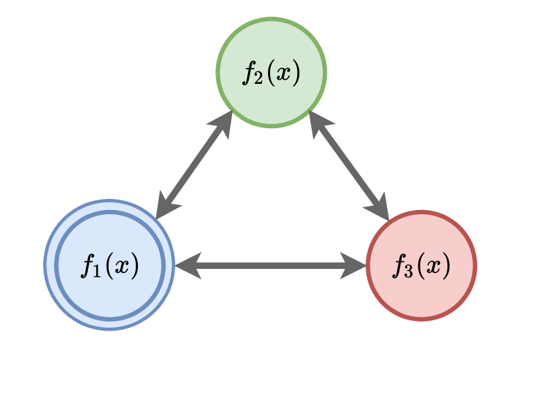
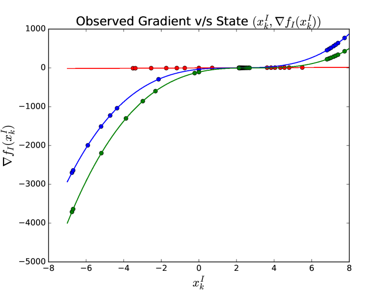
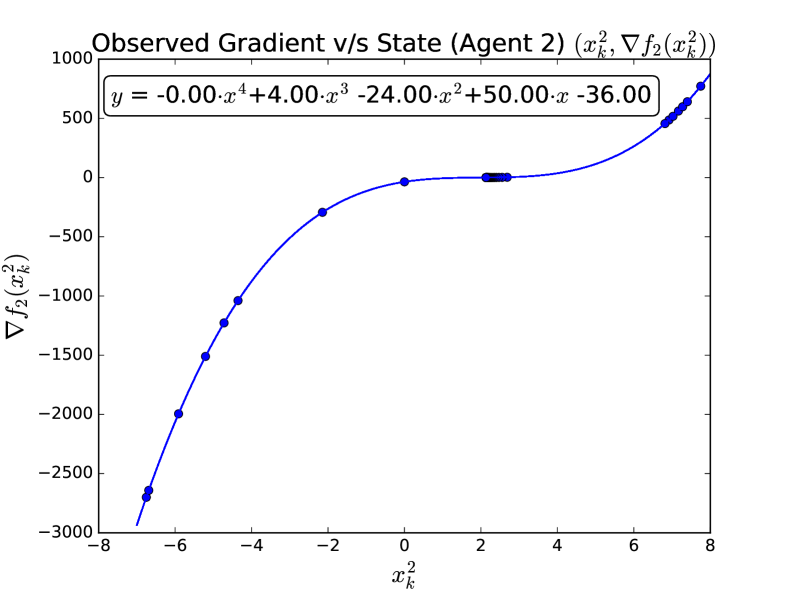
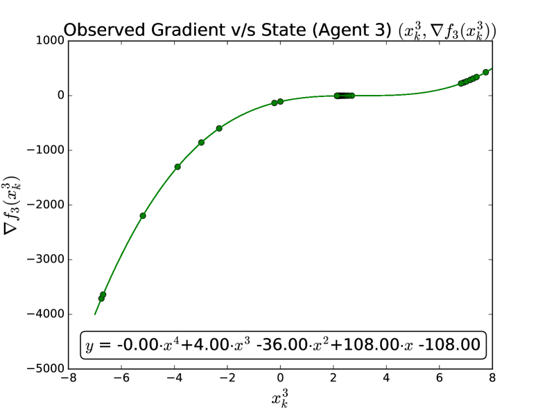
Let us consider a distributed optimization problem over a network with three nodes in a fully connected topology (Figure 1(a)). The private objective functions for each of the nodes are . The system of agents tries to find an optima of using distributed optimization protocol (for deterministic objective functions) from [53] or [23]. Agent 1 is a strong PC adversary (as shown in Figure 1(a) with two concentric circles in blue) with private objective function . The adversary has complete knowledge of state evolution of all states () and the network connectivity. Agent 1 can estimate both and , since it is privy to the states, network structure and step sizes. The adversary can estimate the gradient function using polynomial interpolation or polynomial regression. Integrating the gradient provides the objective functions and with an ambiguity of a constant term.
In this example we show a successful attack from a strong PC adversary. Distributed optimization protocol from [53] is executed for 300 iterations. The system of agents correctly solves the optimization problem. During the execution, adversary observes the state evolution and using its knowledge of the protocol and the network structure, it estimates gradient values at discrete iterates. Agent 1 uses least squares polynomial fitting (numpy.polyfit) to guess the gradient function based on estimated gradient and iterate pairs. This gradient function is further integrated to obtain the objective function. In this attack, the functions guessed by the adversary are tabulated in Table 1. The adversary is successful in uncovering objective functions and (with an ambiguity in the constant term).
| Problem 1 | |||
|---|---|---|---|
| True Obj. Function, | Estimated Obj. Function, | Ambiguity | |
| Known to Adversary | - | ||
3 Privacy Preserving Distributed Optimization Algorithm
We present privacy preserving distributed optimization algorithm inspired by secure multiparty aggregation algorithm in [27]. We present a two step protocol. In the first step we perform a secure exchange of arbitrarily generated functions and then use these functions to transform the private objective functions. The second step involves an interleaved consensus and projected gradient algorithm [53]. Our algorithm, differs from popular distributed gradient descent protocols, in the sense that it involves the objective function being transformed enabling us to provide privacy guarantees. The convergence analysis used here (presented in [53]) is also novel in the sense that it proves convergence of a distributed projected gradient descent algorithm for a convex aggregate of non-convex functions.
Each agent is endowed with a private objective function . Now consider that each agent, , arbitrarily generates functions corresponding to each of its neighbors (). All agents, , then securely share with their neighbors . Any agent , thus has access to functions that it has shared with neighbors, for , and functions that it has received from neighbors, for such that . This step is followed by obfuscation of the private objective function using the arbitrarily generated functions . Every agent transforms its objective function by adding all the arbitrary functions that it has received from its neighbors and subtracting all the arbitrary functions transmitted to the neighbors, and arrives to the obfuscated objective function ,
| (3) |
The objective obfuscation step is followed by iterative distributed projected gradient algorithm similar to [23, 53]. The algorithm is formally presented as Algorithm 1. The interleaved consensus and projected gradient algorithm involves two operations. The first operation in the algorithm is to fuse information from the neighbors and build an estimate of average of the parameter vector. A doubly stochastic matrices , with the property that any entry is greater than zero if and only if and can communicate with each other, is used for information fusion. Also, we assume that all non-zero entries are lower bounded by , i.e. if then for some constant . We can write the fusion step as,
| (4) |
The information aggregation step is followed by projected gradient step and it is formally written as,
| (5) |
where, is the projection operator onto set (cf. [57]), and is the learning rate. Projected gradient descent is a well known iterative gradient based method that guarantees convergence to optimum under reducing learning rate () [58]. We assume that the monotonically non-increasing learning rate (step-size, ) possesses the following properties,
| (6) |
Remark 1 (Invariant Aggregate).
Every arbitrary function gets added to the objective function of and gets subtracted from the objective function of . Then, it is easy to see that the sum of obfuscated objective functions, , is the same as the sum of private objective functions, , i.e. the aggregate is invariant under this transformation.
| (7) |
Remark 2 (Computational Complexity).
Secure transmissions are computationally complex and expensive. It is one of the major drawbacks of cryptographic approaches to privacy and security [41]. Although, our algorithm involves a secure transmission, it is worth noting that this exchange happens only once, at the start of the algorithm. The iterative consensus and projected gradient steps (Lines 5 - 10 of Algorithm 1) belong to the category of standard iterative distributed optimization algorithms that are known to be computationally inexpensive. Our algorithm does not involve any additional computational overhead due to privacy.
3.1 Generating Arbitrary Functions
We claim that using obfuscated functions instead of original functions , the agents expose only and can hide the original objective functions. We will now build intuition for selecting the arbitrarily generated functions . We know that any agent has access to the following quantities: Original objective function, , functions shared by agent to neighbors, (controlled by agent ), and functions received by agent from neighbors, (controlled by agent ). Clearly, if any agent wishes to hide its objective functions, it needs to be smart in generating .
Assumption 3.
is an additive Abelian group.
For the purpose of discussion below, the admissible function set, (Definition 1), is assumed to satisfy the following axioms. These axioms (A1-A5) are called Abelian axioms; and set and operator that satisfies the Abelian axioms, forms an algebraic structure called Additive Abelian Group denoted by . If the commutativity of the operator is not established, would simply be an additive group [59] [60].
-
A1
The admissible function set is closed under addition.
-
A2
There exists an element , such that, for any , .
-
A3
For every element , there exists such that, .
-
A4
For all , holds.
-
A5
For all , holds.
Example 2 (Bounded Degree Polynomials).
The set of all polynomials of degree less than or equal to is an admissible function set (if denotes a -degree polynomial in , then ). Consider two polynomials in of degree and (), denoted by and where for all . Note, and the closure axiom A1 is satisfied. The zero element corresponding to is a polynomial with all coefficients () being zero. The inverse element corresponding to is a polynomial with . A4 and A5 are trivially satisfied for polynomials. Thus, is an additive Abelian group.
Example 3 (Even Degree Polynomials).
The set of polynomials with even degrees upper bounded by is an admissible function set, . Additive closure, associativity and commutativity can be easily proved. The zero element is just an even degree polynomial with zero coefficients and inverse element is another polynomial with coefficients .
Using the definition and closure properties of the admissible set (due to being an additive Abelian group), we can clearly see that if functions , for all (, ) pairs, then . Another important consideration for selecting , comes from technical assumption 2. The arbitrary functions are so selected that the obfuscated functions satisfy Assumptions 2, i.e. the obfuscated functions should have bounded gradients and must have Lipschitz gradients. It is clear from the above arguments that the strategy of generating functions is problem specific and needs to be looked at on individually.
4 Convergence Analysis and Privacy Results
In this section, we prove the convergence of Algorithm 1, present precise privacy claims and provide proofs.
4.1 Convergence Analysis
Each of the obfuscated objective functions are possibly non-convex functions with a convex aggregate ( is convex, as noted in Remark 1). Convergence results developed in [53] show that Algorithm 1 correctly minimizes convex aggregate of non-convex functions (and hence accurately solves the optimization problem in (2)).
Theorem 1 (Theorem 5 and Claim 1, [53]).
-
Proof:
The proof follows as per the proof for Theorem 5 in [53].
4.2 Privacy Guarantees
We first establish a connectivity condition on the underlying communication topology. Note that we only need strong connectedness for convergence. The following conditions will be used to characterize graph topologies for which privacy guarantees can be provided. We begin with the definition of vertex connectivity and use it to define admissible topologies.
Definition 3 (Vertex Connectivity , [61]).
The vertex connectivity of a connected graph is the minimum number of vertices whose deletion would increase the number of connected components.
Definition 4 (-admissible topology).
A graph is called -admissible if its vertex connectivity is greater than , i.e. .
We use a result from Whitney [62] that relates the vertex connectivity (), the edge connectivity () and the minimum degree of the graph (). We will use this result to obtain a inequality on the minimum degree of a -admissible graph.
Theorem 2 (Whitney, [62]).
For any arbitrary graph , .
We know that for a -admissible graph, , along with the above result we get, . This condition is necessary to ensure the privacy of individual objective functions777We will characterize a few failure scenarios (loss of privacy) including the one with presence of nodes that have degree less than . This is, however, not the only loss of privacy scenario.. Topology being -admissible is necessary and sufficient to ensure privacy of additive objective functions of type , where .
We now formally state the privacy guarantee for our privacy preserving distributed optimization algorithm. As described in Section 2.1, strong PC adversarial coalition has access to parameter vectors (from all agents) and the underlying graph topology. The problem is assumed to satisfy Assumptions 1 and 2 for correctness of the algorithm.
Theorem 3.
-
Proof:
We present a constructive method to show that given an execution (and corresponding observations), any guess of objective functions (, such that the sum of functions is ) made by the coalition is equally likely.
We conservatively assume that the adversary can observe the obfuscated functions, , the private objective functions of the coalition members () and arbitrary functions transmitted from and received by each of the coalition members, and ( and , for all ). Since the adversaries also follow the same protocol (Algorithm 1), the coalition is also aware of the fact that the private objective functions have been obfuscated by function sharing approach (Eq. 3).
Clearly, one can rewrite this transformation approach, using signed incidence matrix of bidirectional graph [61] [63].
| (8) |
where, is a vector of obfuscated functions for , and is a vector of private (true) objective functions, . , where (of dimension ) is the incidence matrix of a directed graph obtained by considering only one of the directions of every bidirectional edge in graph 888This represents an orientation of graph [61].. Each column of represents a directed communication link between any two agents. Hence, any bidirectional edge between agents and is represented as two directed links, to , and to and corresponds to two columns in . R represents a vector consisting of functions . Each entry in vector , function corresponds to a column of which, in turn corresponds to link ; and similarly, function corresponds to a different column of which, in turn corresponds to link . Note that row of column vector corresponds to column of incidence matrix .
We will show that, two different sets of true objective functions ( and ) and correspondingly two different set of arbitrary functions ( and ), can lead to exactly same execution and observations for the adversaries999f and are dissimilar and arbitrarily different.. We want to show that both these cases can result in same obfuscated objective functions. That is,
| (9) |
We will show that given any set of private objective functions , suitably selecting arbitrary functions corresponding to links incident at “good” agents, it is possible to make indistinguishable from original private objective functions , solely based on the execution observed by the adversaries. We do so by determining entries of G, which are arbitrary functions that are dissimilar from when and are both “good”. The design such that the obfuscated objective functions are the same for both situations.
Since adversaries observe arbitrary functions corresponding to edges incident to and from them, we set the arbitrary functions corresponding to edges incident on adversaries as and arbitrary functions corresponding to edges incident away the adversary as (where and , for all ). Now, we define as the vector containing all elements of except those corresponding to the edges incident to and from the adversaries101010The only entries of , that are undecided at this stage are included in . These are functions such that , are both “good”.. Similarly, we define to be the new incidence matrix obtained after deleting all edges that are incident on the adversaries (i.e. deleting columns corresponding to the links incident on adversaries, from the old incidence matrix ). We subtract and () by subtracting them from (in Eq. 9) to get effective function difference denoted by as follows,
| (10) | |||||
| (11) | |||||
where, if entries of were fixed111111Total number of edges incident to and from adversaries is . We fixed them to be the same as corresponding entries from , since the coalition can observe them. then is a vector and is a matrix with dimension . The columns deleted from correspond to the edges that are incident to and from the adversaries. Hence, represents the incidence of a graph with these edges deleted.
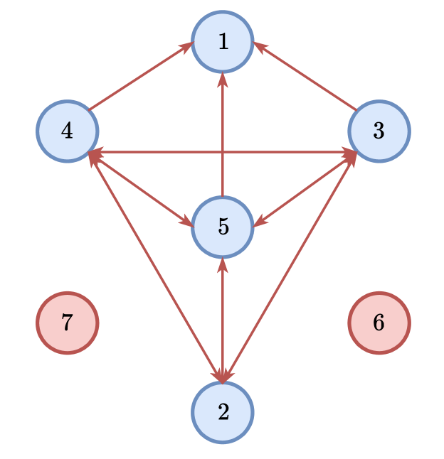
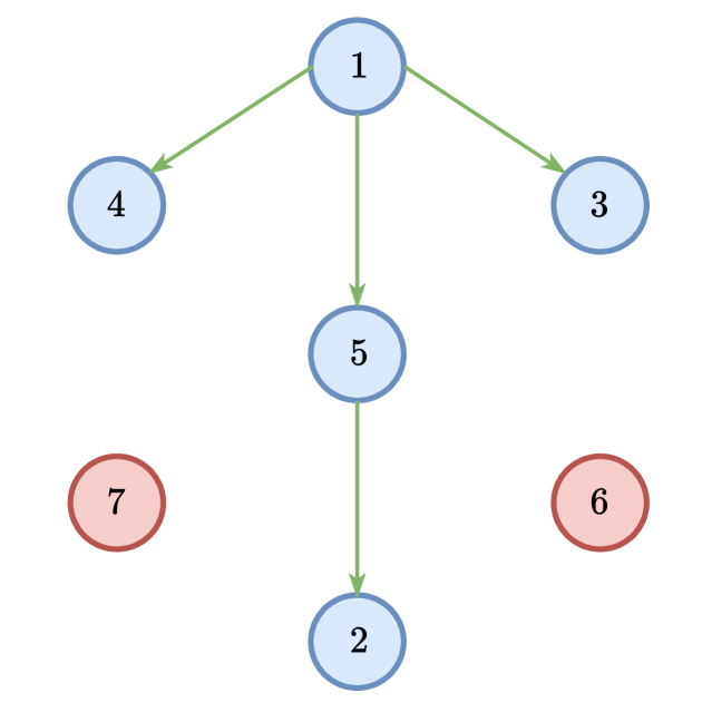
We know from the -admissibility of the graph, that connects all the non-adversarial agents into a connected component121212The adversarial nodes become disconnected due to the deletion of edges incident on adversaries (previous step).. Since, the remaining edges form a connected component, the edges can be split into two groups. A group with edges that form a spanning tree over the good nodes (agents) and all other edges in the other group (see Remark 3 and Figure 2). Let represent the incidence matrix131313Its columns correspond to the edges that form spanning tree. of the spanning tree and represents the arbitrary functions corresponding to the edges of the spanning tree. represents the incidence matrix formed by all other edges and represents the arbitrary functions related to all other edges.
| (12) |
We now arbitrary assign functions to elements of (as per Section 3.1) and then compute the arbitrary weights for . We know that the columns of are linearly independent, since is the incidence matrix of a spanning tree (cf. Lemma 2.5 in [64]). Hence, the left pseudoinverse141414 represents the pseudoinverse of matrix . of exists; and , giving us the solution for 151515An alternate way to look at this would be to see that represents the edge Laplacian [65] of the spanning tree. The edge Laplacian of an acyclic graph is non-singular and this also proves that left-pseudoinverse of exists..
| (13) |
Using the construction shown above, for any we can construct G such that the execution as seen by adversaries is exactly the same as the original problem where the objective is f and the arbitrary functions are R. A strong PC coalition cannot distinguish between two executions involving and f. Hence, no coalition can estimate ().
Remark 3 (Method for Constructing ).
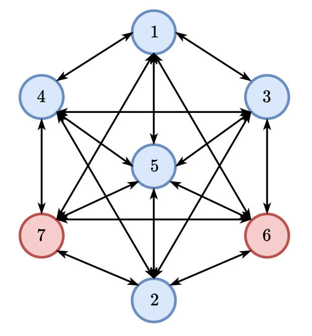
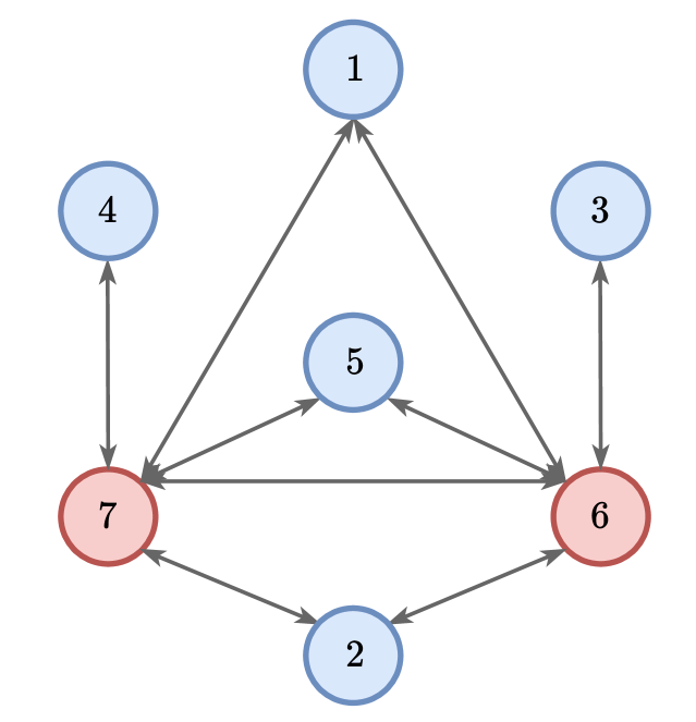
We present an example for the construction used in the above proof. Let us consider a system of agents communicating under a -admissible topology (see Figure 2(a)). A coalition of two PC adversaries (, ) is a part of the system. We can divide the task of constructing into three steps -
-
1.
Fix and (links incident on adversaries) to be the corresponding entries in ,
-
2.
Arbitrarily select the functions corresponding to non spanning tree edges (), and
-
3.
Solve for the functions corresponding to the spanning tree () using Eq. 13.
We first, follow the Step 1 and fix and (where and , for all ). Step 1 follows form the fact that the adversaries observe and , and hence they need to be same in both executions. This is followed by substituting the known entries in and subtract them from the left hand side as shown in Eq. 11. This corresponds to the deletion of all incoming and outgoing edges from the adversaries. The incidence matrix of this new graph is denoted by . The edges in the new graph can be decomposed into two groups - a set containing edges that form a spanning tree and a set that contains all other edges. This is seen in Figure 2(c) where the red edges are all the remaining links (incidence matrix, ); and Figure 2(d) where the green edges form a spanning tree (incidence matrix, ) with Agent 1 as the root and all other “good” agents as its leaves (agents 2, 3, 4, 5). We now arbitrarily select (Step-2) followed by solving for using Eq. 13 (Step-3). This completes construction of .
Example 4.
The privacy preserving optimization algorithm completely obfuscates the true objective functions (topology as shown in Figure 1(a)). We can have, for arbitrarily large number of problems, executions that are exactly same. For instance consider three agents with one adversary (Agent 1). We show that for two different sets of objective functions and 161616The two problems are restricted to have, ., there exists two sets of arbitrarily functions, , such that and , while the adversaries observe the same execution. Column 1 of Table 2 shows the objective functions for two distributed optimization problems. Now we consider two sets of arbitrarily functions, , as seen in Column 2. Observe that the obfuscated objective functions for both problems are exactly the same (Column 3), giving rise to identical executions (iterations) and the quantities observed by the adversary ( and ) are the same for both problems. This results in the inability of the adversary to distinguish between the two different optimization problems.
| Problem 1 | ||
|---|---|---|
| Problem 2 | ||
Theorem 3 states that none of the private objective functions can be meaningfully recovered (Definition 2). However, we can further talk about the privacy of the overall aggregate function, , and the aggregate of objective functions belonging to “good” agents, , under relaxed requirements (like allowing ambiguity in the constant term). We also allow the coalition to run numerical schemes like polynomial regression on observed quantities. With these added assumptions we can claim that a coalition may uncover (not necessarily) the overall aggregate and the aggregate of objective functions private to “good” agents.
Remark 4 (Privacy of ).
The invariance of aggregate is described in Remark 1. Clearly, if the coalition can extract via a numerical scheme (like polynomial regression) albeit with ambiguity in the constant term, then by simply adding all together, the coalition can estimate with uncertainty in the constant term.
Remark 5 (Privacy of ).
We know from Remark 4 that the coalition can estimate and the coalition already has access to the objective functions of the adversaries. Hence, the coalition can estimate using the relation . The coalition can estimate with ambiguity in constant term.
4.3 Loss of Privacy
Theorem 3 clearly characterizes the conditions on communication topology for privacy preservation. The -admissibility condition is both necessary and sufficient for privacy of Algorithm 1. In this section we characterize certain topologies that (do not satisfy -admissibility condition) and are prone to specific types of attacks.
-
•
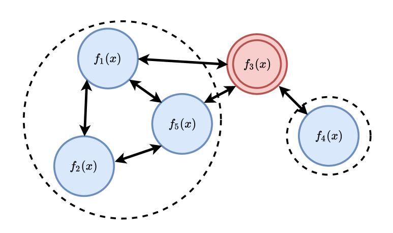
Loss of individual privacy - If the degree of one or more nodes is less than , then those agents are susceptible to privacy loss and a coalition may uncover their objective functions. Figure 3(a) shows a system of five agents () with one adversary (, ) and its communication topology is not -admissible. Agent 4 has a degree deficiency. Since the adversary can observe all the arbitrary functions (, ) used by Agent 4 for obfuscating its objective function, the objective function of Agent 4 () is vulnerable to privacy loss from the adversary.
-
•
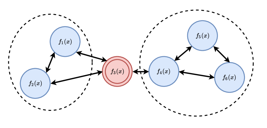
Loss of group privacy - If the vertex is only -admissible and the coalition is a of size , then there exists cases where the coalition can effectively uncover sum of objective functions of a set of agents (group). Figure 3(b) shows a system with six agents () with one adversary (, ) under a -admissible topology. The objective function sums, and are susceptible to privacy loss from the adversary.
5 Simulation Results
In this section, we show that the privacy preserving optimization algorithm in Section 3 solves the learning problem correctly. We consider a network of connected agents as shown in Figure 1(a). Each agent is endowed with a private objective function, given by , and . The system tries to optimize the additive aggregate, . The aggregate function achieves optimum (minimum) at . Agents implement the privacy preserving distributed optimization protocol presented as Algorithm 1. The agents share their states (model parameters) with neighbors. States received from other agents are fused using a doubly-stochastic matrix . The learning step is given by a monotonically decreasing, non-summable but square summable sequence, .
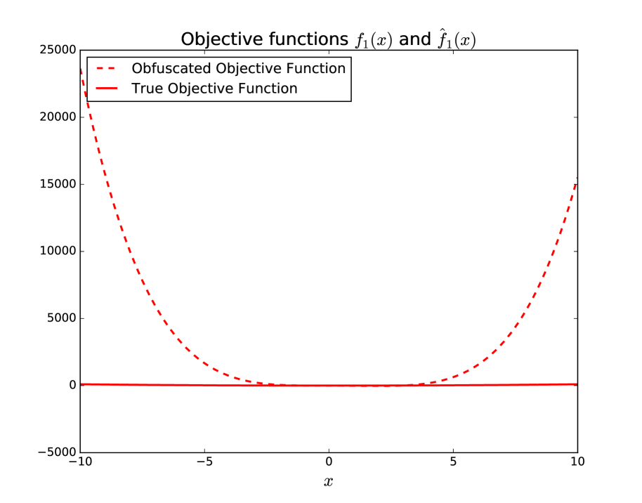
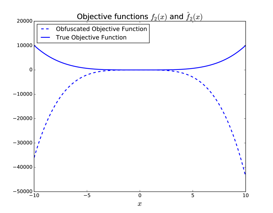
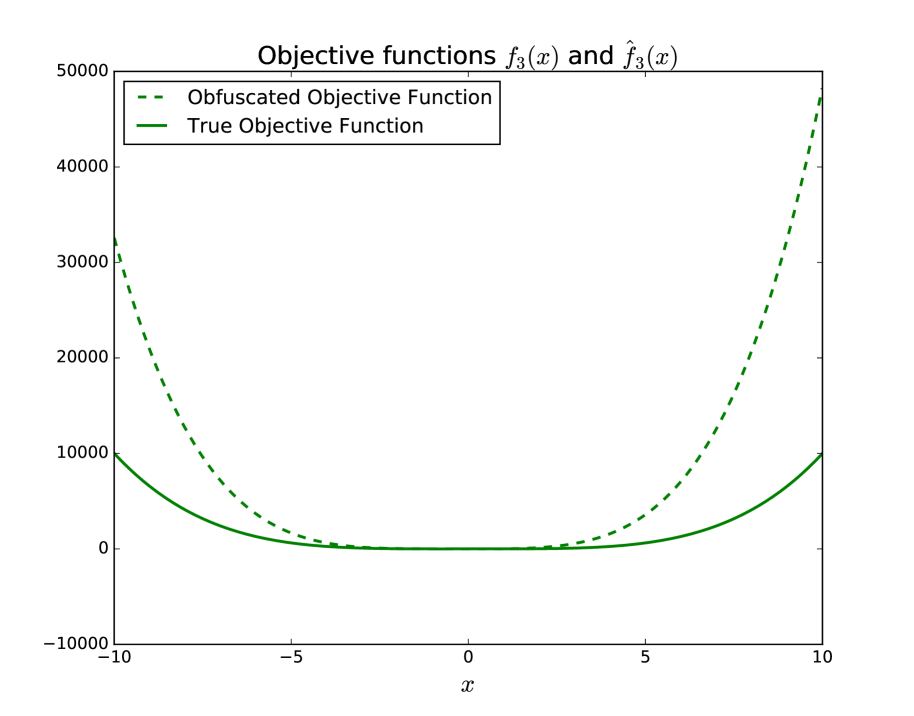
We consider arbitrarily generated function in Table 2 (Problem 1). The obfuscated objective functions are given by (Column 3),
It can be easily verified that the aggregate function is an invariant (Remark 1), . Note, that transformed problem falls under the “distributed optimization of a convex aggregate of non-convex functions” framework, presented in [53]. Figure 4(a), 4(b), and 4(c) shows the effect of obfuscation using arbitrary random functions on the private objective function . As seen in Figure 4, the private objective function and obfuscated functions are different from each other.
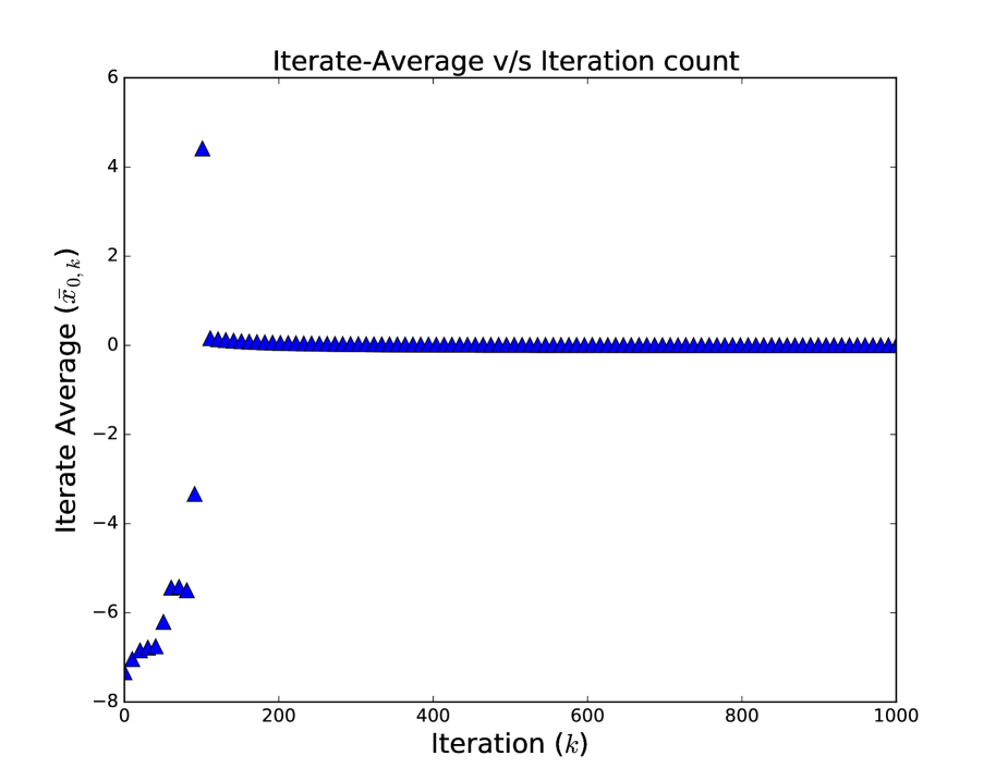
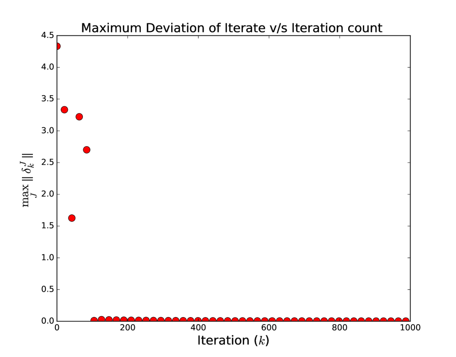
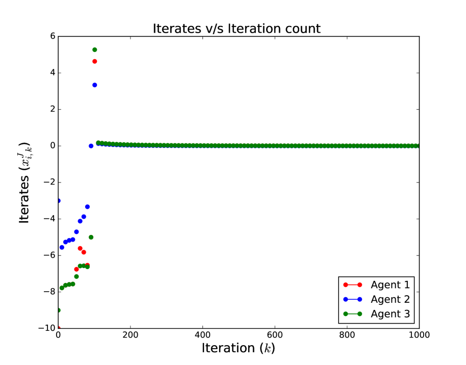
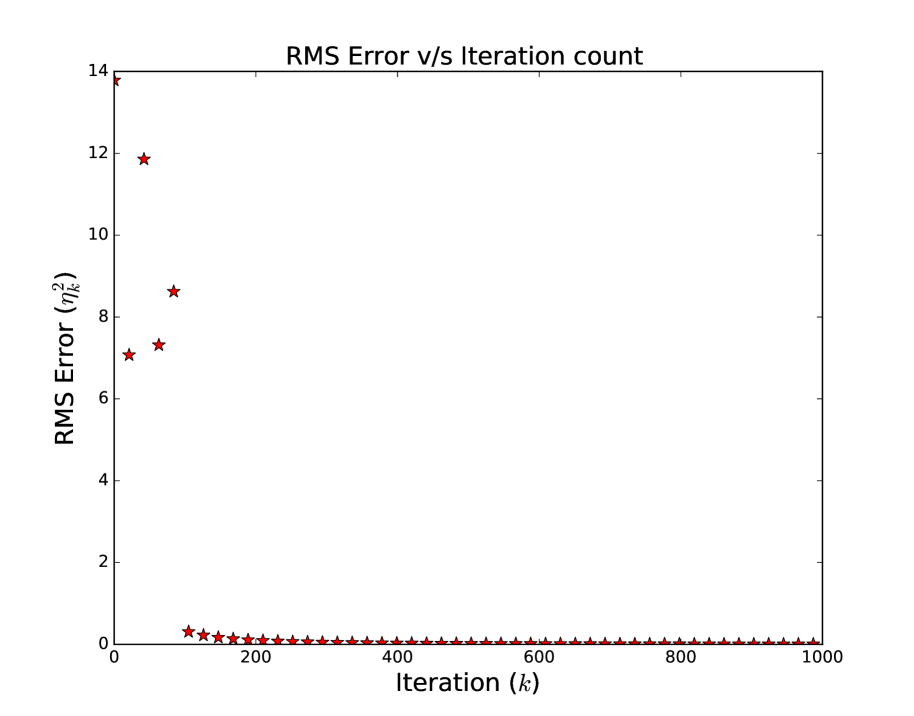
The iterate-average () is plotted in Figure 5(a). The iterate average converges to the optimal point of . Figure 5(b) plots the maximum deviation () of an iterate from the iterate average. The reduction in maximum deviation shows that all the agents converge to the iterate average. Figure 5(c) plots the iterates of each agent with respect to the iteration count. Figure 5(d) decrease in the RMS error ().
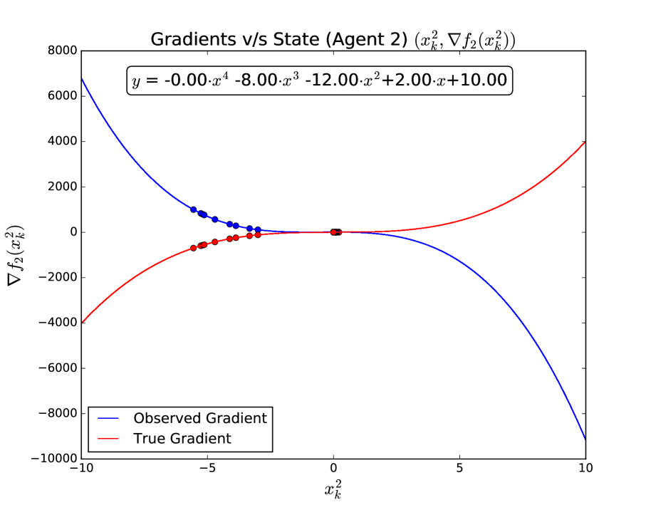
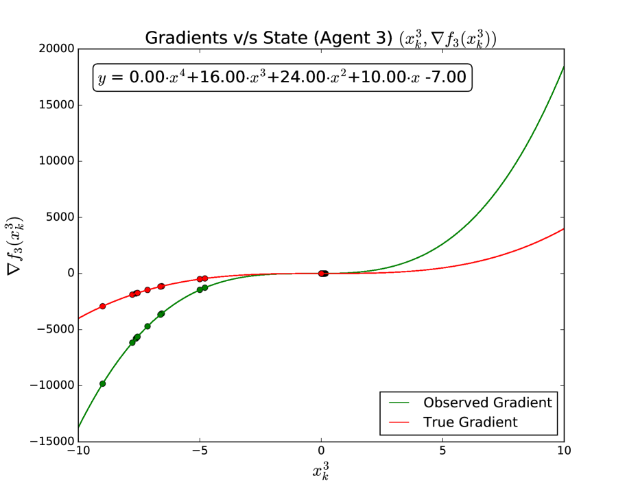
Note that the observed gradient is drastically different from the true gradient. This ensures that even a strong PC adversary can estimate only the obfuscated function. The private objective function remains hidden and an adversary cannot uncover any private objective function.
6 Conclusion
In this report, we present a privacy preserving algorithm for distributed optimization over networks. We show that a secure function sharing approach can be used to obfuscate private objective functions and protect them from adversarial estimation. We define privacy of individual objective functions, in the context of distributed optimization problems, as the inability of an adversary to reduce ambiguity between any arbitrarily guessed (feasible) candidate function. We use vertex connectivity () to characterize graphs that allow Algorithm 1 to be privacy preserving against a coalition of adversaries, in the sense that any arbitrary guess of the objective functions made by the coalition is equally consistent. We prove that the function sharing strategy for privacy preserving distributed optimization preserves privacy under an -admissible graph topology and show correctness, convergence and privacy claims through an example and simulations.
References
- [1] M. Abadi, A. Chu, I. Goodfellow, H. B. McMahan, I. Mironov, K. Talwar, and L. Zhang, “Deep learning with differential privacy,” arXiv preprint arXiv:1607.00133, 2016.
- [2] S. Boyd, N. Parikh, E. Chu, B. Peleato, and J. Eckstein, “Distributed optimization and statistical learning via the alternating direction method of multipliers,” Foundations and Trends® in Machine Learning, vol. 3, no. 1, pp. 1–122, 2011.
- [3] T. Kraska, A. Talwalkar, J. C. Duchi, R. Griffith, M. J. Franklin, and M. I. Jordan, “Mlbase: A distributed machine-learning system.,” in CIDR, vol. 1, pp. 2–1, 2013.
- [4] M. Li, D. G. Andersen, A. J. Smola, and K. Yu, “Communication efficient distributed machine learning with the parameter server,” in Advances in Neural Information Processing Systems 27, pp. 19–27, Curran Associates, Inc., 2014.
- [5] M. Li, L. Zhou, Z. Yang, A. Li, and F. Xia, “Parameter Server for Distributed Machine Learning,” Big Learning Workshop, pp. 1–10, 2013.
- [6] I. Cano, M. Weimer, D. Mahajan, C. Curino, and G. M. Fumarola, “Towards geo-distributed machine learning,” arXiv preprint arXiv:1603.09035, 2016.
- [7] A. Nedić and A. Olshevsky, “Distributed Optimization Over Time-Varying Directed Graphs,” IEEE Transactions on Automatic Control, vol. 60, no. 3, pp. 601–615, 2015.
- [8] S. Gade and N. Vaidya, “Distributed optimization for client-server architecture with negative gradient weights,” arXiv preprint arXiv:1608.03866, 2016.
- [9] Y. Nesterov, “Efficiency of coordinate descent methods on huge-scale optimization problems,” SIAM Journal on Optimization, vol. 22, no. 2, pp. 341–362, 2012.
- [10] J. Liu and S. J. Wright, “Asynchronous stochastic coordinate descent: Parallelism and convergence properties,” SIAM Journal on Optimization, vol. 25, no. 1, pp. 351–376, 2015.
- [11] A. Agarwal and J. C. Duchi, “Distributed delayed stochastic optimization,” in Advances in Neural Information Processing Systems, pp. 873–881, 2011.
- [12] C. Singh, A. Nedić, and R. Srikant, “Random Block-Coordinate Gradient Projection Algorithms,” in 53rd IEEE Conference on Decision and Control, pp. 185–190, 2014.
- [13] A. Nedić and A. Ozdaglar, “On the rate of convergence of distributed subgradient methods for multi-agent optimization,” Proceedings of the IEEE Conference on Decision and Control, vol. 54, no. 1, pp. 4711–4716, 2007.
- [14] A. Nedić, “Asynchronous broadcast-based convex optimization over a network,” IEEE Transactions on Automatic Control, vol. 56, no. 6, pp. 1337–1351, 2011.
- [15] A. Nedić and A. Olshevsky, “Distributed Optimization Over Time-Varying Directed Graphs,” IEEE Transactions on Automatic Control, vol. 60, no. 3, pp. 601–615, 2015.
- [16] R. Zhang and J. T. Kwok, “Asynchronous distributed admm for consensus optimization.,” in ICML, pp. 1701–1709, 2014.
- [17] Z. Huang, S. Mitra, and N. Vaidya, “Differentially private distributed optimization,” in Proceedings of the 2015 International Conference on Distributed Computing and Networking, p. 4, ACM, 2015.
- [18] M. Rabbat and R. Nowak, “Distributed optimization in sensor networks,” in Proceedings of the 3rd international symposium on Information processing in sensor networks, pp. 20–27, ACM, 2004.
- [19] M. Zhu and S. Martínez, “On distributed convex optimization under inequality and equality constraints,” IEEE Transactions on Automatic Control, vol. 57, no. 1, pp. 151–164, 2012.
- [20] S. Sra, S. Nowozin, and S. J. Wright, Optimization for machine learning. MIT Press, 2012.
- [21] C. N. Hadjicostis, N. H. Vaidya, and A. D. Domínguez-García, “Robust distributed average consensus via exchange of running sums,” IEEE Transactions on Automatic Control, vol. 61, no. 6, pp. 1492–1507, 2016.
- [22] E. Wei and A. Ozdaglar, “On the o (1= k) convergence of asynchronous distributed alternating direction method of multipliers,” in Global Conference on Signal and Information Processing (GlobalSIP), 2013 IEEE, pp. 551–554, IEEE, 2013.
- [23] S. S. Ram, A. Nedić, and V. V. Veeravalli, “Distributed stochastic subgradient projection algorithms for convex optimization,” Journal of optimization theory and applications, vol. 147, no. 3, pp. 516–545, 2010.
- [24] S. S. Ram, A. Nedić, and V. V. Veeravalli, “Incremental stochastic subgradient algorithms for convex optimization,” SIAM Journal on Optimization, vol. 20, no. 2, pp. 691–717, 2009.
- [25] L. Su and N. H. Vaidya, “Fault-tolerant multi-agent optimization: Optimal iterative distributed algorithms,” in Proceedings of the 2016 ACM Symposium on Principles of Distributed Computing, pp. 425–434, ACM, 2016.
- [26] R. Shokri and V. Shmatikov, “Privacy-Preserving Deep Learning,” Proceedings of the 22nd ACM SIGSAC Conference on Computer and Communications Security - CCS ’15, pp. 1310–1321, 2015.
- [27] E. A. Abbe, A. E. Khandani, and A. W. Lo, “Privacy-preserving methods for sharing financial risk exposures,” The American Economic Review, vol. 102, no. 3, pp. 65–70, 2012.
- [28] M. Alizadeh, T.-H. Chang, and A. Scaglione, “Grid integration of distributed renewables through coordinated demand response,” in 2012 IEEE 51st IEEE Conference on Decision and Control (CDC), pp. 3666–3671, IEEE, 2012.
- [29] F. Pasqualetti, F. Dörfler, and F. Bullo, “Cyber-physical security via geometric control: Distributed monitoring and malicious attacks,” in 2012 IEEE 51st IEEE Conference on Decision and Control (CDC), pp. 3418–3425, IEEE, 2012.
- [30] R. Shokri and V. Shmatikov, “Privacy-preserving deep learning,” in Proceedings of the 22nd ACM SIGSAC Conference on Computer and Communications Security, pp. 1310–1321, ACM, 2015.
- [31] “SwiftKey.” https://swiftkey.com/en. Accessed: 2016-10-16.
- [32] H. B. McMahan, E. Moore, D. Ramage, et al., “Federated learning of deep networks using model averaging,” arXiv preprint arXiv:1602.05629, 2016.
- [33] H. S. Hippert, C. E. Pedreira, and R. C. Souza, “Neural networks for short-term load forecasting: A review and evaluation,” IEEE Transactions on power systems, vol. 16, no. 1, pp. 44–55, 2001.
- [34] J. Vaidya, “Privacy-preserving linear programming,” in Proceedings of the 2009 ACM symposium on Applied Computing, pp. 2002–2007, ACM, 2009.
- [35] Y. Hong, J. Vaidya, N. Rizzo, and Q. Liu, “Privacy preserving linear programming,” arXiv preprint arXiv:1610.02339, 2016.
- [36] J. Cortes, S. Martinez, and F. Bullo, “Spatially-distributed coverage optimization and control with limited-range interactions,” ESAIM: Control, Optimisation and Calculus of Variations, vol. 11, no. 4, pp. 691–719, 2005.
- [37] W. Ren, R. W. Beard, and E. M. Atkins, “A survey of consensus problems in multi-agent coordination,” in Proceedings of the 2005, American Control Conference, 2005., pp. 1859–1864, IEEE, 2005.
- [38] R. Olfati-Saber, “Distributed tracking for mobile sensor networks with information-driven mobility,” in 2007 American Control Conference, pp. 4606–4612, IEEE, 2007.
- [39] S. Gade and A. Joshi, “Heterogeneous uav swarm system for target search in adversarial environment,” in 2013 International Conference on Control Communication and Computing (ICCC), pp. 358–363, Dec 2013.
- [40] S. Gade, A. A. Paranjape, and S.-J. Chung, “Herding a flock of birds approaching an airport using an unmanned aerial vehicle,” in AIAA Guidance, Navigation, and Control Conference, p. 1540, AIAA, 2015.
- [41] P. C. Weeraddana, G. Athanasiou, C. Fischione, and J. S. Baras, “Per-se privacy preserving solution methods based on optimization,” in Proceedings of the 52nd IEEE Conference on Decision and Control (CDC), pp. 206–211, 2013.
- [42] P. C. Weeraddana, G. Athanasiou, M. Jakobsson, C. Fischione, and J. S. Baras, “On the privacy of optimization approaches,” arXiv preprint arXiv:1210.3283, 2012.
- [43] O. Goldreich, Foundations of cryptography: volume 2, basic applications. Cambridge university press, 2009.
- [44] S. Goldwasser, “Multi party computations: past and present,” in Proceedings of the sixteenth annual ACM symposium on Principles of distributed computing, pp. 1–6, ACM, 1997.
- [45] B. Pinkas, “Cryptographic techniques for privacy-preserving data mining,” ACM Sigkdd Explorations Newsletter, vol. 4, no. 2, pp. 12–19, 2002.
- [46] A. Bednarz, Methods for two-party privacy-preserving linear programming. PhD thesis, 2012.
- [47] S. Han, U. Topcu, and G. J. Pappas, “Differentially private distributed constrained optimization,” IEEE Transactions on Automatic Control, vol. PP, no. 99, pp. 1–1, 2016.
- [48] E. Nozari, P. Tallapragada, and J. Cortés, “Differentially private distributed convex optimization via functional perturbation,” arXiv preprint arXiv:1512.00369, 2015.
- [49] O. L. Mangasarian, “Privacy-preserving horizontally partitioned linear programs,” Optimization Letters, vol. 6, no. 3, pp. 431–436, 2012.
- [50] C. Wang, K. Ren, and J. Wang, “Secure and practical outsourcing of linear programming in cloud computing,” in INFOCOM, 2011 Proceedings IEEE, pp. 820–828, IEEE, 2011.
- [51] J. Dreier and F. Kerschbaum, “Practical privacy-preserving multiparty linear programming based on problem transformation,” in Privacy, Security, Risk and Trust (PASSAT) and 2011 IEEE Third Inernational Conference on Social Computing (SocialCom), 2011 IEEE Third International Conference on, pp. 916–924, IEEE, 2011.
- [52] Y. Lou, L. Yu, and S. Wang, “Privacy preservation in distributed subgradient optimization algorithms,” arXiv preprint arXiv:1512.08822, 2015.
- [53] S. Gade and N. Vaidya, “Distributed optimization of convex sum of non-convex functions,” arXiv preprint arXiv:1608.05401, 2016.
- [54] L. Lamport, R. Shostak, and M. Pease, “The byzantine generals problem,” ACM Transactions on Programming Languages and Systems (TOPLAS), vol. 4, no. 3, pp. 382–401, 1982.
- [55] A. Shamir, “How to share a secret,” Communications of the ACM, vol. 22, no. 11, pp. 612–613, 1979.
- [56] C. Li and P. Zhou, “Differentially private distributed online learning,” arXiv preprint arXiv:1505.06556, 2015.
- [57] D. P. Bertsekas, A. Nedić, A. E. Ozdaglar, et al., Convex analysis and optimization. Athena Scientific, 2003.
- [58] D. P. Bertsekas, “On the Goldstein-Levitin-Polyak gradient projection method,” Automatic Control, IEEE Transactions on, vol. 21, no. 2, pp. 174–184, 1976.
- [59] T. W. Judson, “Abstract algebra,” 2010.
- [60] J. Gallian, Contemporary abstract algebra. Cengage Learning, 2016.
- [61] C. Godsil and G. F. Royle, Algebraic graph theory, vol. 207. Springer Science & Business Media, 2013.
- [62] H. Whitney, “Congruent graphs and the connectivity of graphs,” American Journal of Mathematics, vol. 54, no. 1, pp. 150–168, 1932.
- [63] R. Diestel, “Graph theory. 2005,” Grad. Texts in Math, vol. 101, 2005.
- [64] R. B. Bapat, Graphs and Matrices. Springer, 2010.
- [65] D. Zelazo, A. Rahmani, and M. Mesbahi, “Agreement via the edge laplacian,” in Decision and Control, 2007 46th IEEE Conference on, pp. 2309–2314, IEEE, 2007.
