Tunable Efficient Unitary Neural Networks (EUNN) and their application to RNNs

Abstract

Using unitary (instead of general) matrices in artificial neural networks (ANNs) is a promising way to solve the gradient explosion/vanishing problem, as well as to enable ANNs to learn long-term correlations in the data. This approach appears particularly promising for Recurrent Neural Networks (RNNs). In this work, we present a new architecture for implementing an Efficient Unitary Neural Network (EUNNs); its main advantages can be summarized as follows. Firstly, the representation capacity of the unitary space in an EUNN is fully tunable, ranging from a subspace of SU(N) to the entire unitary space. Secondly, the computational complexity for training an EUNN is merely $\mathcal{O}(1)$ per parameter. Finally, we test the performance of EUNNs on the standard copying task, the pixel-permuted MNIST digit recognition benchmark as well as the Speech Prediction Test (TIMIT). We find that our architecture significantly outperforms both other state-of-the-art unitary RNNs and the LSTM architecture, in terms of the final performance and/or the wall-clock training speed. EUNNs are thus promising alternatives to RNNs and LSTMs for a wide variety of applications.

1 Introduction

Deep Neural Networks (LeCun et al., 2015) have been successful on numerous difficult machine learning tasks, including image recognition(Krizhevsky et al., 2012; Donahue et al., 2015), speech recognition(Hinton et al., 2012) and natural language processing(Collobert et al., 2011; Bahdanau et al., 2014; Sutskever et al., 2014). However, deep neural networks can suffer from vanishing and exploding gradient problems(Hochreiter, 1991; Bengio et al., 1994), which are known to be caused by matrix eigenvalues far from unity being raised to large powers. Because the severity of these problems grows with the the depth of a neural network, they are particularly grave for Recurrent Neural Networks (RNNs), whose recurrence can be equivalent to thousands or millions of equivalent hidden layers.

Several solutions have been proposed to solve these problems for RNNs. Long Short Term Memory (LSTM) networks (Hochreiter & Schmidhuber, 1997), which help RNNs contain information inside hidden layers with gates, remains one of the the most popular RNN implementations. Other recently proposed methods such as GRUs(Cho et al., 2014) and Bidirectional RNNs (Berglund et al., 2015) also perform well in numerous applications. However, none of these approaches has fundamentally solved the vanishing and exploding gradient problems, and gradient clipping is often required to keep gradients in a reasonable range.

A recently proposed solution strategy is using orthogonal hidden weight matrices or their complex generalization (unitary matrices) (Saxe et al., 2013; Le et al., 2015; Arjovsky et al., 2015; Henaff et al., 2016), because all their eigenvalues will then have absolute values of unity, and can safely be raised to large powers. This has been shown to help both when weight matrices are initialized to be unitary (Saxe et al., 2013; Le et al., 2015) and when they are kept unitary during training, either by restricting them to a more tractable matrix subspace (Arjovsky et al., 2015) or by alternating gradient-descent steps with projections onto the unitary subspace (Wisdom et al., 2016).

In this paper, we will first present an Efficient Unitary Neural Network (EUNN) architecture that parametrizes the entire space of unitary matrices in a complete and computationally efficient way, thereby eliminating the need for time-consuming unitary subspace-projections. Our architecture has a wide range of capacity-tunability to represent subspace unitary models by fixing some of our parameters; the above-mentioned unitary subspace models correspond to special cases of our architecture. We also implemented an EUNN with an earlier introduced FFT-like architecture which efficiently approximates the unitary space with minimum number of required parameters(Mathieu & LeCun, 2014b).

We then benchmark EUNN’s performance on both simulated and real tasks: the standard copying task, the pixel-permuted MNIST task, and speech prediction with the TIMIT dataset (Garofolo et al., 1993). We show that our EUNN algorithm with an $\mathcal{O}(N)$ hidden layer size can compute up to the entire $N\times N$ gradient matrix using $\mathcal{O}(1)$ computational steps and memory access per parameter. This is superior to the $\mathcal{O}(N)$ computational complexity of the existing training method for a full-space unitary network (Wisdom et al., 2016) and $\mathcal{O}(\log N)$ more efficient than the subspace Unitary RNN(Arjovsky et al., 2015).

2 Background

2.1 Basic Recurrent Neural Networks

A recurrent neural network takes an input sequence and uses the current hidden state to generate a new hidden state during each step, memorizing past information in the hidden layer. We first review the basic RNN architecture.

Consider an RNN updated at regular time intervals $t=1,2,...$ whose input is the sequence of vectors ${\bf x}^{(t)}$ whose hidden layer ${\bf h}^{(t)}$ is updated according to the following rule:

$${\bf h}^{(t)}=\sigma({\bf U}{\bf x}^{(t)}+\bm{W}{\bf h}^{(t-1)}),$$ (1)

where $\sigma$ is the nonlinear activation function. The output is generated by

$${\bf y}^{(t)}={\bf W}{\bf h}^{(t)}+{\bf b},$$ (2)

where ${\bf b}$ is the bias vector for the hidden-to-output layer. For $t=0$, the hidden layer $\mathbf{h^{(0)}}$ can be initialized to some special vector or set as a trainable variable. For convenience of notation, we define ${\bf z}^{(t)}={\bf U}{\bf x}^{(t)}+{\bf W}{\bf h}^{(t-1)}$ so that ${\bf h}^{(t)}=\sigma({{\bf z}^{(t)}})$.

2.2 The Vanishing and Exploding Gradient Problems

When training the neural network to minimize a cost function $C$ that depends on a parameter vector ${\bf a}$, the gradient descent method updates this vector to ${\bf a}-\lambda\frac{\partial C}{\partial{\bf a}}$, where $\lambda$ is a fixed learning rate and $\frac{\partial C}{\partial{\bf a}}\equiv\nabla C$. For an RNN, the vanishing or exploding gradient problem is most significant during back propagation from hidden to hidden layers, so we will only focus on the gradient for hidden layers. Training the input-to-hidden and hidden-to-output matrices is relatively trivial once the hidden-to-hidden matrix has been successfully optimized.

In order to evaluate $\frac{\partial C}{\partial W_{ij}}$, one first computes the derivative $\frac{\partial C}{\partial h^{(t)}}$ using the chain rule:

$$\frac{\partial C}{\partial{\bf h}^{(t)}} = \frac{\partial C}{\partial{\bf h}^{(T)}}\frac{\partial{\bf h}^{(T)}}{\partial{\bf h}^{(t)}}$$ (3)

$$= \frac{\partial C}{\partial{\bf h}^{(T)}}\prod_{k=t}^{T-1}\frac{\partial{\bf h}^{(k+1)}}{\partial{\bf h}^{(k)}}$$ (4)

$$= \frac{\partial C}{\partial{\bf h}^{(T)}}\prod_{k=t}^{T-1}{\bf D}^{(k)}{{\bf W}},$$ (5)

where ${\bf D}^{(k)}={\rm diag}\{\sigma^{\prime}({\bf U}{\bf x}^{(k)}+{\bf W}{\bf h}^{(k-1)})\}$ is the Jacobian matrix of the pointwise nonlinearity. For large times $T$, the term $\prod{\bf W}$ plays a significant role. As long as the eigenvalues of ${\bf D}^{(k)}$ are of order unity, then if ${\bf W}$ has eigenvalues $\lambda_{i}\gg 1$, they will cause gradient explosion $|\frac{\partial C}{\partial{\bf h}^{(T)}}|\rightarrow\infty$, while if ${\bf W}$ has eigenvalues $\lambda_{i}\ll 1$, they can cause gradient vanishing, $|\frac{\partial C}{\partial{\bf h}^{(T)}}|\rightarrow 0$. Either situation prevents the RNN from working efficiently.

3 Unitary RNNs

3.1 Partial Space Unitary RNNs

In a breakthrough paper, Arjovsky, Shah & Bengio (Arjovsky et al., 2015) showed that unitary RNNs can overcome the exploding and vanishing gradient problems and perform well on long term memory tasks if the hidden-to-hidden matrix in parametrized in the following unitary form:

$${\bf W}={\bf D}_{3}{\bf T}_{2}\mathcal{F}^{-1}{\bf D}_{2}{\bm{\Pi}}{\bf T}_{1}\mathcal{F}{\bf D}_{1}.$$ (6)

Here ${\bf D}_{1,2,3}$ are diagonal matrices with each element $e^{i\omega_{j}},j=1,2,\cdots,n$. ${\bf T}_{1,2}$ are reflection matrices, and ${\bf T}=I-2\frac{\widehat{\bf v}\widehat{\bf v}^{\dagger}}{||\widehat{\bf v}||^{2}}$, where $\widehat{\bf v}$ is a vector with each of its entries as a parameter to be trained. $\bm{\Pi}$ is a fixed permutation matrix. $\mathcal{F}$ and $\mathcal{F}^{-1}$ are Fourier and inverse Fourier transform matrices respectively. Since each factor matrix here is unitary, the product ${\bf W}$ is also a unitary matrix.

This model uses $\mathcal{O}(N)$ parameters, which spans merely a part of the whole $\mathcal{O}(N^{2})$-dimensional space of unitary $N\times N$ matrices to enable computational efficiency. Several subsequent papers have tried to expand the space to $\mathcal{O}(N^{2})$ in order to achieve better performance, as summarized below.

3.2 Full Space Unitary RNNs

In order to maximize the power of Unitary RNNs, it is preferable to have the option to optimize the weight matrix ${\bf W}$ over the full space of unitary matrices rather than a subspace as above. A straightforward method for implementing this is by simply updating ${\bf W}$ with standard back-propagation and then projecting the resulting matrix (which will typically no longer be unitary) back onto to the space of unitary matrices. Defining ${\bf G}_{ij}\equiv\frac{\partial{C}}{\partial{W_{ij}}}$ as the gradient with respect to ${\bf W}$, this can be implemented by the procedure defined by (Wisdom et al., 2016):

$${\bf A}^{(t)} \equiv {{\bf G}^{(t)}}^{\dagger}{\bf W}^{(t)}-{{\bf W}^{(t)}}^{\dagger}{\bf G}^{(k)},$$ (7)

$${\bf W}^{(t+1)} \equiv \left({\bf I}+\frac{\lambda}{2}{\bf A}^{(t)}\right)^{-1}\left({\bf I}-\frac{\lambda}{2}{\bf A}^{(t)}\right){\bf W}^{(t)}.$$ (8)

This method shows that full space unitary networks are superior on many RNN tasks (Wisdom et al., 2016). A key limitation is that the back-propation in this method cannot avoid $N$-dimensional matrix multiplication, incurring $\mathcal{O}(N^{3})$ computational cost.

4 Efficient Unitary Neural Network (EUNN) Architectures

In the following, we first describe a general parametrization method able to represent arbitrary unitary matrices with up to $N^{2}$ degrees of freedom. We then present an efficient algorithm for this parametrization scheme, requiring only $\mathcal{O}(1)$ computational and memory access steps to obtain the gradient for each parameter. Finally, we show that our scheme performs significantly better than the above mentioned methods on a few well-known benchmarks.

4.1 Unitary Matrix Parametrization

Any $N\times N$ unitary matrix ${\bf W}_{N}$ can be represented as a product of rotation matrices $\{{\bf R}_{ij}\}$ and a diagonal matrix ${\bf D}$, such that ${\bf W}_{N}={\bf D}\prod_{i=2}^{N}\prod_{j=1}^{i-1}{\bf R}_{ij}$, where ${\bf R}_{ij}$ is defined as the $N$-dimensional identity matrix with the elements $R_{ii}$, $R_{ij}$, $R_{ji}$ and $R_{jj}$ replaced as follows (Reck et al., 1994; Clements et al., 2016):

$$\begin{pmatrix}R_{ii}&R_{ij}\\ R_{ji}&R_{jj}\\ \end{pmatrix}=\begin{pmatrix}e^{i\phi_{ij}}\cos\theta_{ij}&-e^{i\phi_{ij}}\sin\theta_{ij}\\ \sin\theta_{ij}&\cos\theta_{ij}\\ \end{pmatrix}.$$ (9)

where $\theta_{ij}$ and $\phi_{ij}$ are unique parameters corresponding to $\mathbf{R_{ij}}$. Each of these matrices performs a $U(2)$ unitary transformation on a two-dimensional subspace of the N-dimensional Hilbert space, leaving an $(N-2)$-dimensional subspace unchanged. In other words, a series of $U(2)$ rotations can be used to successively make all off-diagonal elements of the given $N\times N$ unitary matrix zero. This generalizes the familiar factorization of a 3D rotation matrix into 2D rotations parametrized by the three Euler angles. To provide intuition for how this works, let us briefly describe a simple way of doing this that is similar to Gaussian elimination by finishing one column at a time. There are infinitely many alternative decomposition schemes as well; Fig. 1 shows two that are particularly convenient to implement in software (and even in neuromorphic hardware (Shen et al., 2016)). The unitary matrix ${\bf W}_{N}$ is multiplied from the right by a succession of unitary matrices ${\bf R}_{Nj}$ for $j=N-1,\cdots,1$. Once all elements of the last row except the one on the diagonal are zero, this row will not be affected by later transformations. Since all transformations are unitary, the last column will then also contain only zeros except on the diagonal:

$${\bf W}_{N}{\bf R}_{N,N-1}{\bf R}_{N,N-2}\cdot\cdot{\bf R}_{N,1}=\begin{pmatrix}{\bf W}_{N-1}&0\\ 0&e^{iw_{N}}\end{pmatrix}$$ (10)

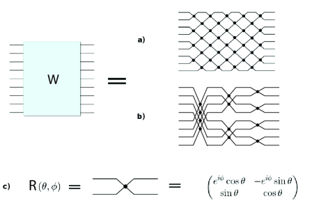
Figure 1: Unitary matrix decomposition: An arbitrary unitary matrix ${\bf W}$ can be decomposed (a) with the square decomposition method of Clements et al. (Clements et al., 2016) discussed in section 4.2; or approximated (b) by the Fast Fourier Transformation(FFT) style decomposition method (Mathieu & LeCun, 2014b) discussed in section 4.3. Each junction in the a) and b) graphs above represent the U(2) matrix as shown in c).

The effective dimensionality of the the matrix ${\bf W}$ is thus reduced to $N-1$. The same procedure can then be repeated $N-1$ times until the effective dimension of ${\bf W}$ is reduced to 1, leaving us with a diagonal matrix:

$${\bf W}_{N}{\bf R}_{N,N-1}{\bf R}_{N,N-2}\cdots{\bf R}_{i,j}{\bf R}_{i,j-1}\cdots{\bf R}_{3,1}{\bf R}_{2,1}={\bf D},$$ (11)

where ${\bf D}$ is a diagonal matrix whose diagonal elements are $e^{iw_{j}}$, from which we can write the direct representation of ${\bf W}_{N}$ as

$${\bf W}_{N} ={\bf D}{\bf R}_{2,1}^{-1}{\bf R}_{3,1}^{-1}\dots\bf R_{N,N-2}^{-1}{\bf R}_{N,N-1}^{-1}$$ (12)

$$={\bf D}{\bf R}^{\prime}_{2,1}{\bf R}^{\prime}_{3,1}\dots\bf R^{\prime}_{N,N-2}{\bf R}^{\prime}_{N,N-1}.$$

where

$${\bf R}^{\prime}_{ij}={\bf R}(-\theta_{ij},-\phi_{ij})={\bf R}(\theta_{ij},\phi_{ij})^{-1}={\bf R}_{ij}^{-1}$$ (13)

This parametrization thus involves $N(N-1)/2$ different $\theta_{ij}$-values, $N(N-1)/2$ different $\phi_{ij}$-values and $N$ different $w_{i}$-values, combining to $N^{2}$ parameters in total and spans the entire unitary space. Note we can always fix a portion of our parameters, to span only a subset of unitary space – indeed, our benchmark test below will show that for certain tasks, full unitary space parametrization is not necessary.

4.2 Tunable space implementation

The representation in Eq. 12 can be made more compact by reordering and grouping specific rotational matrices, as was shown in the optical community (Reck et al., 1994; Clements et al., 2016) in the context of universal multiport interferometers. For example (Clements et al., 2016), a unitary matrix can be decomposed as

$${\bf W}_{N} = {\bf D}\left({\bf R}_{1,2}^{(1)}{\bf R}_{3,4}^{(1)}\dots\bf R_{N/2-1,N/2}^{(1)}\right)$$ (14)

$$\times\left({\bf R}_{2,3}^{(2)}{\bf R}_{4,5}^{(2)}\dots\bf R_{N/2-2,N/2-1}^{(2)}\right)$$

$$\times\dots$$

$$= {\bf D}{\bf F}_{A}^{(1)}{\bf F}_{B}^{(2)}\dots\bf F_{B}^{(L)},$$

where every

$$\mathbf{F}_{A}^{(l)}={\bf R}_{1,2}^{(l)}{\bf R}_{3,4}^{(l)}\dots\bf R_{N/2-1,N/2}^{(l)}$$

is a block diagonal matrix, with $N$ angle parameters in total, and

$$\mathbf{F}_{B}^{(l)}={\bf R}_{2,3}^{(l)}{\bf R}_{4,5}^{(l)}\dots\bf R_{N/2-2,N/2-1}^{(l)}$$

with $N-1$ parameters, as is schematically shown in Fig. 1a. By choosing different values for $L$ , ${\bf W}_{N}$ will span a different subspace of the unitary space. Specifically,when $L=N$, ${\bf W}_{N}$ will span the entire unitary space.

Following this physics-inspired scheme, we decompose our unitary hidden-to-hidden layer matrix ${\bf W}$ as

$$\mathbf{W}=\mathbf{D}\mathbf{F}_{A}^{(1)}\mathbf{F}_{B}^{(2)}\mathbf{F}_{A}^{(3)}\mathbf{F}_{B}^{(4)}\cdots\mathbf{F}_{B}^{(L)}.$$ (15)

4.3 FFT-style approximation

Inspired by (Mathieu & LeCun, 2014a), an alternative way to organize the rotation matrices is implementing an FFT-style architecture. Instead of using adjacent rotation matrices, each $\mathbf{F}$ here performs a certain distance pairwise rotations as shown in Fig. 1b:

$$\mathbf{W}=\mathbf{D}\mathbf{F}_{1}\mathbf{F}_{2}\mathbf{F}_{3}\mathbf{F}_{4}\cdots\mathbf{F}_{\log(N)}.$$ (16)

The rotation matrices in $\mathbf{F}_{i}$ are performed between pairs of coordinates

$$(2pk+j,p(2k+1)+j)$$ (17)

where $p=\frac{N}{2^{i}}$, $k\in\{0,...,2^{i-1}\}$ and $j\in\{1,...,p\}$. This requires only $\log(N)$ matrices, so there are a total of $N\log(N)/2$ rotational pairs. This is also the minimal number of rotations that can have all input coordinates interacting with each other, providing an approximation of arbitrary unitary matrices.

4.4 Efficient implementation of rotation matrices

To implement this decomposition efficiently in an RNN, we apply vector element-wise multiplications and permutations: we evaluate the product $\mathbf{F}{\bf x}$ as

$$\mathbf{F}\mathbf{x}=\mathbf{v_{1}}*\mathbf{x}+\mathbf{v_{2}}*\mathrm{permute}(\mathbf{x})$$ (18)

where $*$ represents element-wise multiplication, $\mathbf{F}$ refers to general rotational matrices such as $\mathbf{F}_{A/B}$ in Eq. 14 and $\mathbf{F}_{i}$ in Eq. 16. For the case of the tunable-space implementation, if we want to implement $\mathbf{F}_{A}^{(l)}$ in Eq. 14, we define $\mathbf{v}$ and the permutation as follows:

$$\mathbf{v_{1}}=(e^{i\phi_{1}^{(l)}}\cos\theta_{1}^{(l)},\cos\theta_{1}^{(l)},e^{i\phi_{2}^{(l)}}\cos\theta_{2}^{(l)},\cos\theta_{2}^{(l)},\cdots)$$

$$\mathbf{v_{2}}=(-e^{i\phi_{1}^{(l)}}\sin\theta_{1}^{(l)},\sin\theta_{1}^{(l)},-e^{i\phi_{2}^{(l)}}\sin\theta_{2},\sin\theta_{2}^{(l)},\cdots)$$

$$\mathrm{permute}(\mathbf{x})=(x_{2},x_{1},x_{4},x_{3},x_{6},x_{5},\cdots).$$

For the FFT-style approach, if we want to implement $\mathbf{F}_{1}$ in Eq  16, we define $\mathbf{v}$ and the permutation as follows:

$$\mathbf{v_{1}}=(e^{i\phi_{1}^{(l)}}\cos\theta_{1}^{(l)},e^{i\phi_{2}^{(l)}}\cos\theta_{2}^{(l)},\cdots,\cos\theta_{1}^{(l)},\cos\theta_{2}^{(l)},\cdots)$$

$$\mathbf{v_{2}}=(-e^{i\phi_{1}^{(l)}}\sin\theta_{1}^{(l)},-e^{i\phi_{2}^{(l)}}\sin\theta_{2},\cdots,\sin\theta_{1}^{(l)},\sin\theta_{2}^{(l)},\cdots)$$

$$\mathrm{permute}(\mathbf{x})=(x_{\frac{n}{2}+1},x_{\frac{n}{2}+2}\cdots x_{n},x_{1},x_{2}\cdots).$$

In general, the pseudocode for implementing operation $\mathbf{F}$ is as follows:

Algorithm 1 Efficient implementation for $\mathbf{F}$ with parameter $\theta_{i}$ and $\phi_{i}$.

  Input: input $\mathbf{x}$, size $N$; parameters $\mathbf{\theta}$ and $\mathbf{\phi}$, size $N/2$; constant permuatation index list $\mathbf{ind_{1}}$ and $\mathbf{ind_{2}}$.

  Output: output $\mathbf{y}$, size $N$.

  $\mathbf{v_{1}}$ $\leftarrow$ concatenate($\cos\mathbf{\theta}$, $\cos\mathbf{\theta}$ * $\exp(i\mathbf{\phi})$)

  $\mathbf{v_{2}}$ $\leftarrow$ concatenate($\sin\mathbf{\theta}$, - $\sin\mathbf{\theta}$ * $\exp(i\mathbf{\phi})$)

  $\mathbf{v_{1}}$ $\leftarrow$ $\mathrm{permute}(\mathbf{v_{1}},\mathbf{ind_{1}})$

  $\mathbf{v_{2}}$ $\leftarrow$ $\mathrm{permute}(\mathbf{v_{2}},\mathbf{ind_{1}})$

  $\mathbf{y}$ $\leftarrow$ $\mathbf{v_{1}}*\mathbf{x}+\mathbf{v_{2}}*\mathrm{permute}(\mathbf{x},\mathbf{ind_{2}})$

Note that $\mathbf{ind_{1}}$ and $\mathbf{ind_{2}}$ are different for different $\mathbf{F}$.

From a computational complexity viewpoint, since the operations $*$ and $\mathrm{permute}$ take $\mathcal{O}(N)$ computational steps, evaluating $\mathbf{F}\mathbf{x}$ only requires $\mathcal{O}(N)$ steps. The product $\mathbf{D}\mathbf{x}$ is trivial, consisting of an element-wise vector multiplication. Therefore, the product $\mathbf{W}\mathbf{x}$ with the total unitary matrix $\mathbf{W}$ can be computed in only $\mathcal{O}(NL)$ steps, and only requires $\mathcal{O}(NL)$ memory access (for full-space implementation $L=N$, for FFT-style approximation gives $L=\log N$). A detailed comparison on computational complexity of the existing unitary RNN architectures is given in Table 1.

Table 1: Performance comparison of four Recurrent Neural Network algorithms: URNN (Arjovsky et al., 2015), PURNN (Wisdom et al., 2016), and EURNN (our algorithm). $T$ denotes the RNN length and $N$ denotes the hidden state size. For the tunable-style EURNN, $L$ is an integer between 1 and $N$ parametrizing the unitary matrix capacity.

Model	Time complexity of one	number of parameters	Transition matrix
	online gradient step	in the hidden matrix	search space
URNN	$\mathcal{O}(TN\log N)$	$\mathcal{O}(N)$	subspace of $\mathbf{U}(N)$
PURNN	$\mathcal{O}(TN^{2}+N^{3})$	$\mathcal{O}(N^{2})$	full space of $\mathbf{U}(N)$
EURNN (tunable style)	$\mathcal{O}(TNL)$	$\mathcal{O}(NL)$	tunable space of $\mathbf{U}(N)$
EURNN (FFT style)	$\mathcal{O}(TN\log N)$	$\mathcal{O}(N\log N)$	subspace of $\mathbf{U}(N)$

4.5 Nonlinearity

We use the same nonlinearity as (Arjovsky et al., 2015):

$$(\mathrm{modReLU}(\mathbf{z},\mathbf{b}))_{i}=\frac{z_{i}}{|z_{i}|}*\mathrm{ReLU}(|z_{i}|+b_{i})$$ (19)

where the bias vector $\mathbf{b}$ is a shared trainable parameter, and $|z_{i}|$ is the norm of the complex number $z_{i}$.

For real number input, $\mathrm{modReLU}$ can be simplified to:

$$(\mathrm{modReLU}(\mathbf{z},\mathbf{b}))_{i}=\mathrm{sign}(z_{i})*\mathrm{ReLU}(|z_{i}|+b_{i})$$ (20)

where $|z_{i}|$ is the absolute value of the real number $z_{i}$.

We empirically find that this nonlinearity function performs the best. We believe that this function possibly also serves as a forgetting filter that removes the noise using the bias threshold.

5 Experimental tests of our method

In this section, we compare the performance of our Efficient Unitary Recurrent Neural Network (EURNN) with

1. an LSTM RNN (Hochreiter & Schmidhuber, 1997),

2. a Partial Space URNN (Arjovsky et al., 2015), and

3. a Projective full-space URNN (Wisdom et al., 2016).

All models are implemented in both Tensorflow and Theano, available from https://github.com/jingli9111/EUNN-tensorflow and https://github.com/iguanaus/EUNN-theano.

5.1 Copying Memory Task

We compare these networks by applying them all to the well defined Copying Memory Task (Hochreiter & Schmidhuber, 1997; Arjovsky et al., 2015; Henaff et al., 2016). The copying task is a synthetic task that is commonly used to test the network’s ability to remember information seen $T$ time steps earlier.

Specifically, the task is defined as follows (Hochreiter & Schmidhuber, 1997; Arjovsky et al., 2015; Henaff et al., 2016). An alphabet consists of symbols $\{a_{i}\}$, the first $n$ of which represent data, and the remaining two representing “blank” and “start recall”, respectively; as illustrated by the following example where $T=20$ and $M=5$:

Input:  BACCA--------------------:----
Output: -------------------------BACCA

In the above example, $n=3$ and $\{a_{i}\}=\{A,B,C,-,:\}$. The input consists of $M$ random data symbols ($M=5$ above) followed by $T-1$ blanks, the “start recall” symbol and $M$ more blanks. The desired output consists of $M+T$ blanks followed by the data sequence. The cost function $C$ is defined as the cross entropy of the input and output sequences, which vanishes for perfect performance.

We use $n=8$ and input length $M=10$. The symbol for each input is represented by an $n$-dimensional one-hot vector. We trained all five RNNs for $T=1000$ with the same batch size 128 using RMSProp optimization with a learning rate of 0.001. The decay rate is set to 0.5 for EURNN, and 0.9 for all other models respectively. (Fig. 2). This results show that the EURNN architectures introduced in both Sec.4.2 (EURNN with N=512, selecting L=2) and Sec.4.3 (FFT-style EURNN with N=512) outperform the LSTM model (which suffers from long term memory problems and only performs well on the copy task for small time delays $T$) and all other unitary RNN models, both in-terms of learnability and in-terms of convergence rate. Note that the only other unitary RNN model that is able to beat the baseline for $T=1000$ (Wisdom et al., 2016) is significantly slower than our method.

Moreover, we find that by either choosing smaller $L$ or by using the FFT-style method (so that $\mathbf{W}$ spans a smaller unitary subspace), the EURNN converges toward optimal performance significantly more efficiently (and also faster in wall clock time) than the partial (Arjovsky et al., 2015) and projective (Wisdom et al., 2016) unitary methods. The EURNN also performed more robustly. This means that a full-capacity unitary matrix is not necessary for this particular task.

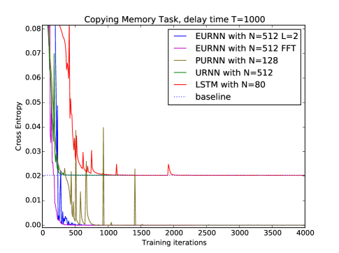
Figure 2: Copying Task for $T=1000$. EURNN corresponds to our algorithm, projective URNN corresponds to algorithm presented in (Wisdom et al., 2016), URNN corresponds to the algorithm presented in (Arjovsky et al., 2015). A useful baseline performance is that of the memoryless strategy, which outputs $M+T$ blanks followed by $M$ random data symbols and produces a cross entropy $C=(M\log{n})/(T+2*M)$. [Note that each iteration for PURNN takes about 32 times longer than for EURNN models, for this particular simulation, so the speed advantage is much greater than apparent in this plot.]

5.2 Pixel-Permuted MNIST Task

The MNIST handwriting recognition problem is one of the classic benchmarks for quantifying the learning ability of neural networks. MNIST images are formed by a 28$\times$28 grayscale image with a target label between 0 and 9.

To test different RNN models, we feed all pixels of the MNIST images into the RNN models in 28$\times$28 time steps, where one pixel at a time is fed in as a floating-point number. A fixed random permutation is applied to the order of input pixels. The output is the probability distribution quantifying the digit prediction. We used RMSProp with a learning rate of 0.0001 and a decay rate of 0.9, and set the batch size to 128.

Table 2: MNIST Task result. EURNN corresponds to our algorithm, PURNN corresponds to algorithm presented in (Wisdom et al., 2016), URNN corresponds to the algorithm presented in (Arjovsky et al., 2015).

Model	hidden size	number of	validation	test
	(capacity)	parameters	accuracy	accuracy
LSTM	80	16k	0.908	0.902
URNN	512	16k	0.942	0.933
PURNN	116	16k	0.922	0.921
EURNN (tunable style)	1024 (2)	13.3k	0.940	0.937
EURNN (FFT style)	512 (FFT)	9.0k	0.928	0.925

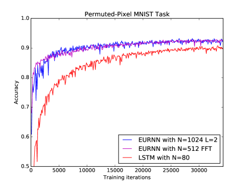
Figure 3: Pixel-permuted MNIST performance on the validation dataset.

As shown in Fig. 3, EURNN significantly outperforms LSTM with the same number of parameters. It learns faster, in fewer iteration steps, and converges to a higher classification accuracy. In addition, the EURNN reaches a similar accuracy with fewer parameters. In Table. 2, we compare the performance of different RNN models on this task.

5.3 Speech Prediction on TIMIT dataset

Table 3: Speech Prediction Task result. EURNN corresponds to our algorithm, projective URNN corresponds to algorithm presented in (Wisdom et al., 2016), URNN corresponds to the algorithm presented in (Arjovsky et al., 2015).

Model	hidden size	number of	MSE	MSE
	(capacity)	parameters	(validation)	(test)
LSTM	64	33k	71.4	66.0
LSTM	128	98k	55.3	54.5
EURNN (tunable style)	128 (2)	33k	63.3	63.3
EURNN (tunable style)	128 (32)	35k	52.3	52.7
EURNN (tunable style)	128 (128)	41k	51.8	51.9
EURNN (FFT style)	128 (FFT)	34k	52.3	52.4

Figure 4: Example spectrograms of ground truth and RNN prediction results from evaluation sets.

We also apply our EURNN to real-world speech prediction task and compare its performance to LSTM. The main task we consider is predicting the log-magnitude of future frames of a short-time Fourier transform (STFT) (Wisdom et al., 2016; Sejdić et al., 2009). We use the TIMIT dataset (Garofolo et al., 1993) sampled at 8 kHz. The audio .wav file is initially diced into different time frames (all frames have the same duration referring to the Hann analysis window below). The audio amplitude in each frame is then Fourier transformed into the frequency domain. The log-magnitude of the Fourier amplitude is normalized and used as the data for training/testing each model. In our STFT operation we uses a Hann analysis window of 256 samples (32 milliseconds) and a window hop of 128 samples (16 milliseconds). The frame prediction task is as follows: given all the log-magnitudes of STFT frames up to time $t$, predict the log-magnitude of the STFT frame at time $t+1$ that has the minimum mean square error (MSE). We use a training set with 2400 utterances, a validation set of 600 utterances and an evaluation set of 1000 utterances. The training, validation, and evaluation sets have distinct speakers. We trained all RNNs for with the same batch size 32 using RMSProp optimization with a learning rate of 0.001, a momentum of 0.9 and a decay rate of 0.1.

The results are given in Table. 3, in terms of the mean-squared error (MSE) loss function. Figure. 4 shows prediction examples from the three types of networks, illustrating how EURNNs generally perform better than LSTMs. Furthermore, in this particular task, full-capacity EURNNs outperform small capacity EURNNs and FFT-style EURNNs.

6 Conclusion

We have presented a method for implementing an Efficient Unitary Neural Network (EUNN) whose computational cost is merely $\mathcal{O}(1)$ per parameter, which is $\mathcal{O}(\log N)$ more efficient than the other methods discussed above. It significantly outperforms existing RNN architectures on the standard Copying Task, and the pixel-permuted MNIST Task using a comparable parameter count, hence demonstrating the highest recorded ability to memorize sequential information over long time periods.

It also performs well on real tasks such as speech prediction, outperforming an LSTM on TIMIT data speech prediction.

We want to emphasize the generality and tunability of our method. The ordering of the rotation matrices we presented in Fig. 1 are merely two of many possibilities; we used it simply as a concrete example. Other ordering options that can result in spanning the full unitary matrix space can be used for our algorithm as well, with identical speed and memory performance. This tunability of the span of the unitary space and, correspondingly, the total number of parameters makes it possible to use different capacities for different tasks, thus opening the way to an optimal performance of the EUNN. For example, as we have shown, a small subspace of the full unitary space is preferable for the copying task, whereas the MNIST task and TIMIT task are better performed by EUNN covering a considerably larger unitary space. Finally, we note that our method remains applicable even if the unitary matrix is decomposed into a different product of matrices (Eq. 12).

This powerful and robust unitary RNN architecture also might be promising for natural language processing because of its ability to efficiently handle tasks with long-term correlation and very high dimensionality.

References

- Arjovsky et al. (2015) Arjovsky, Martin, Shah, Amar, and Bengio, Yoshua. Unitary evolution recurrent neural networks. arXiv preprint arXiv:1511.06464, 2015.
- Bahdanau et al. (2014) Bahdanau, Dzmitry, Cho, Kyunghyun, and Bengio, Yoshua. Neural machine translation by jointly learning to align and translate. arXiv preprint arXiv:1409.0473, 2014.
- Bengio et al. (1994) Bengio, Yoshua, Simard, Patrice, and Frasconi, Paolo. Learning long-term dependencies with gradient descent is difficult. IEEE transactions on neural networks, 5(2):157–166, 1994.
- Berglund et al. (2015) Berglund, Mathias, Raiko, Tapani, Honkala, Mikko, Kärkkäinen, Leo, Vetek, Akos, and Karhunen, Juha T. Bidirectional recurrent neural networks as generative models. In Advances in Neural Information Processing Systems, pp. 856–864, 2015.
- Cho et al. (2014) Cho, Kyunghyun, Van Merriënboer, Bart, Bahdanau, Dzmitry, and Bengio, Yoshua. On the properties of neural machine translation: Encoder-decoder approaches. arXiv preprint arXiv:1409.1259, 2014.
- Clements et al. (2016) Clements, William R., Humphreys, Peter C., Metcalf, Benjamin J., Kolthammer, W. Steven, and Walmsley, Ian A. An optimal design for universal multiport interferometers, 2016. arXiv:1603.08788.
- Collobert et al. (2011) Collobert, Ronan, Weston, Jason, Bottou, Léon, Karlen, Michael, Kavukcuoglu, Koray, and Kuksa, Pavel. Natural language processing (almost) from scratch. Journal of Machine Learning Research, 12(Aug):2493–2537, 2011.
- Donahue et al. (2015) Donahue, Jeffrey, Anne Hendricks, Lisa, Guadarrama, Sergio, Rohrbach, Marcus, Venugopalan, Subhashini, Saenko, Kate, and Darrell, Trevor. Long-term recurrent convolutional networks for visual recognition and description. In Proceedings of the IEEE Conference on Computer Vision and Pattern Recognition, pp. 2625–2634, 2015.
- Garofolo et al. (1993) Garofolo, John S, Lamel, Lori F, Fisher, William M, Fiscus, Jonathon G, and Pallett, David S. Darpa timit acoustic-phonetic continous speech corpus cd-rom. nist speech disc 1-1.1. NASA STI/Recon technical report n, 93, 1993.
- Henaff et al. (2016) Henaff, Mikael, Szlam, Arthur, and LeCun, Yann. Orthogonal rnns and long-memory tasks. arXiv preprint arXiv:1602.06662, 2016.
- Hinton et al. (2012) Hinton, Geoffrey, Deng, Li, Yu, Dong, Dahl, George E, Mohamed, Abdel-rahman, Jaitly, Navdeep, Senior, Andrew, Vanhoucke, Vincent, Nguyen, Patrick, Sainath, Tara N, et al. Deep neural networks for acoustic modeling in speech recognition: The shared views of four research groups. IEEE Signal Processing Magazine, 29(6):82–97, 2012.
- Hochreiter (1991) Hochreiter, Sepp. Untersuchungen zu dynamischen neuronalen netzen. Diploma, Technische Universität München, pp. 91, 1991.
- Hochreiter & Schmidhuber (1997) Hochreiter, Sepp and Schmidhuber, Jürgen. Long short-term memory. Neural computation, 9(8):1735–1780, 1997.
- Krizhevsky et al. (2012) Krizhevsky, Alex, Sutskever, Ilya, and Hinton, Geoffrey E. Imagenet classification with deep convolutional neural networks. In Advances in neural information processing systems, pp. 1097–1105, 2012.
- Le et al. (2015) Le, Quoc V, Jaitly, Navdeep, and Hinton, Geoffrey E. A simple way to initialize recurrent networks of rectified linear units. arXiv preprint arXiv:1504.00941, 2015.
- LeCun et al. (2015) LeCun, Yann, Bengio, Yoshua, and Hinton, Geoffrey. Deep learning. Nature, 521(7553):436–444, 2015.
- Mathieu & LeCun (2014a) Mathieu, Michael and LeCun, Yann. Fast approximation of rotations and hessians matrices. arXiv preprint arXiv:1404.7195, 2014a.
- Mathieu & LeCun (2014b) Mathieu, Michal and LeCun, Yann. Fast approximation of rotations and hessians matrices. CoRR, abs/1404.7195, 2014b. URL http://arxiv.org/abs/1404.7195.
- Reck et al. (1994) Reck, Michael, Zeilinger, Anton, Bernstein, Herbert J., and Bertani, Philip. Experimental realization of any discrete unitary operator. Phys. Rev. Lett., 73:58–61, Jul 1994. doi: 10.1103/PhysRevLett.73.58. URL http://link.aps.org/doi/10.1103/PhysRevLett.73.58.
- Saxe et al. (2013) Saxe, Andrew M, McClelland, James L, and Ganguli, Surya. Exact solutions to the nonlinear dynamics of learning in deep linear neural networks. arXiv preprint arXiv:1312.6120, 2013.
- Sejdić et al. (2009) Sejdić, Ervin, Djurović, Igor, and Jiang, Jin. Time–frequency feature representation using energy concentration: An overview of recent advances. Digital Signal Processing, 19(1):153 – 183, 2009. ISSN 1051-2004. doi: http://dx.doi.org/10.1016/j.dsp.2007.12.004. URL http://www.sciencedirect.com/science/article/pii/S105120040800002X.
- Shen et al. (2016) Shen, Yichen, Harris, Nicholas C, Skirlo, Scott, Prabhu, Mihika, Baehr-Jones, Tom, Hochberg, Michael, Sun, Xin, Zhao, Shijie, Larochelle, Hugo, Englund, Dirk, et al. Deep learning with coherent nanophotonic circuits. arXiv preprint arXiv:1610.02365, 2016.
- Sutskever et al. (2014) Sutskever, Ilya, Vinyals, Oriol, and Le, Quoc V. Sequence to sequence learning with neural networks. In Advances in neural information processing systems, pp. 3104–3112, 2014.
- Wisdom et al. (2016) Wisdom, Scott, Powers, Thomas, Hershey, John, Le Roux, Jonathan, and Atlas, Les. Full-capacity unitary recurrent neural networks. In Advances In Neural Information Processing Systems, pp. 4880–4888, 2016.