A high-fidelity solver for turbulent compressible flows on unstructured meshes

Abstract

We develop a high-fidelity numerical solver for the compressible Navier-Stokes equations, with the main aim of highlighting the predictive capabilities of low-diffusive numerics for flows in complex geometries. The space discretization of the convective terms in the Navier-Stokes equations relies on a robust energy-preserving numerical flux, and numerical diffusion inherited from the AUSM scheme is added limited to the vicinity of shock waves, or wherever spurious numerical oscillations are sensed. The solver is capable of conserving the total kinetic energy in the inviscid limit, and it bears sensibly less numerical diffusion than typical industrial solvers, with incurred greater predictive power, as demonstrated through a series of test cases including DNS, LES and URANS of turbulent flows. Simplicity of implementation in existing popular solvers such as OpenFOAM^® is also highlighted.

1 Introduction

Computational fluid dynamics (CFD) has become a common tool for the prediction of flows of engineering interest. Since the pioneering works of Orszag and Patterson [1], Kim et al. [2], which first showed the potential of computers for high-fidelity prediction of turbulent flows, many studies have appeared in which CFD has been used to tackle fundamental topics in turbulence research [3, 4, 5], and to solve flows of industrial interest [6, 7, 8, 9]. Although CFD is currently used with good degree of success in the routine industrial design process, a large disparity between the accuracy of algorithms used in commercial flow solvers and in academia is still evident. Spectral methods [10], high-order finite difference (FD) methods [11], discretely energy-preserving schemes [12, 13], and accurate explicit time integration [14, 15] are common features of many academic flow solvers. Accurate techniques are also available to capture shock waves in compressible flow, which include the essentially-non-oscillatory schemes and their weighted counterpart, or hybrid schemes [16, 17, 18]. On the other hand, most commercial flow solvers rely on first/second order unstructured finite volume (FV) discretizations, in which the nonlinear terms are typically stabilized through upwinding, and time is advanced through implicit segregated algorithms [19, 20]. In the case of compressible flows, shock-capturing capability is frequently achieved through sturdy but outdated total-variation-diminishing (TVD) schemes, or rougher. A common feature of most commercial flow solvers is the use of severely diffusive numerical algorithms, which may negatively impact the prediction of unsteady turbulent flows, especially in large-eddy simulation (LES) [21]. Although high-accuracy, energy-consistent discretizations can also be applied to unstructured meshes of industrial relevance [22, 23, 24], it appears that the approach has not been incorporated in solvers of common use. The main aim of this work is trying to bridge this gap, by introducing high-fidelity low-diffusive numerical schemes of academic use into existing unstructured flow solvers, with the eventual intent of achieving more accurate prediction of turbulent flows of industrial interest, possibly with little computational overhead. For illustrative purposes, we consider as baseline solver the open-source library OpenFOAM^® [25], which is released under the General Public Licence (GPL), and which has experienced large diffusion in the recent years. The baseline distribution of OpenFOAM^® comes with several compressible flow solvers, of which the most widely used is rhoCentralFoam, relying on full discretization of the convective fluxes through the central TVD scheme of Kurganov and Tadmor [26].

Some attention has been recently devoted to modification of the standard OpenFOAM^® algorithms with the goal of reducing their numerical diffusion [27, 28]. For instance, Vuorinen et al. [27, 28] have introduced a scale-selective mixed central/upwind discretization which is particularly beneficial for LES, especially when coupled with low-diffusion Runge-Kutta time integration. Although the approach limits the amount of numerical diffusion, discrete conservation of total kinetic energy in the inviscid limit is not guaranteed. Shen et al. [29, 30] developed an implicit compressible solver for OpenFOAM^® relying on the AUSM scheme [31] and found similar performances as rhoCentralFoam. Cerminara et al. [32] developed a compressible multi-phase solver for OpenFOAM^® based on the PIMPLE algorithm [20] for the simulation of volcanic ash plumes, which is considerably less diffusive than rhoCentralFoam. Hence, it appears that the OpenFOAM^® community is concerned about numerical diffusion, and some effort is being devoted to trying to minimize it, both for incompressible and compressible flows. Herein we describe an algorithm for the numerical solution of the compressible Navier-Stokes equations which allows to discretely preserve the total flow kinetic energy from convection in the inviscid limit on Cartesian meshes [33], and to maintain good conservation properties also on unstructured triangular meshes through localized augmentation of the numerical flux with the AUSM pressure diffusive flux. Shock-capturing capability is further obtained through localized use of the full AUSM diffusive flux, wherever shocks are sensed. The full algorithm is illustrated in detail in Section 2, and the results of several numerical tests reported in Section 3. Concluding remarks are given in Section 4

2 Numerical algorithm

Figure 1: Computational cell for evaluation of the numerical flux. $ON$ denotes the interface between the owner cell $O$, and the neighbouring cell $N$, and $\mathbf{n}_{ON}$ is the outer normal for $O$. $L$ and $R$ denote limit states at the two sides of the interface ($L\equiv O$, $R\equiv N$ in the case of first-order reconstruction).

We consider the Navier-Stokes equations for a compressible ideal gas, integrated over an arbitrary control volume $V$

$$\frac{\mathrm{d}}{\mathrm{d}t}\int_{V}{\bf u}\,{\mathrm{d}V}+\sum_{i=1}^{3}\int_{\partial V}\left({\bf f}_{i}-{\bf f}^{v}_{i}\right)\,n_{i}\,{\mathrm{d}S}=0,$$ (1)

where ${\bf n}$ is the outward normal, and

$$\mathbf{u}=\begin{Bmatrix}\rho\\ \rho u_{i}\\ \rho E\\ \end{Bmatrix},\quad\mathbf{f}_{i}=\begin{Bmatrix}\rho u_{i}\\ \rho u_{i}u_{j}+p\delta_{ij}\\ \rho u_{i}H\\ \end{Bmatrix},\quad\mathbf{f}_{i}^{v}=\begin{Bmatrix}0\\ \sigma_{ij}\\ \sigma_{ik}u_{k}-q_{i}\\ \end{Bmatrix},$$ (2)

are the vector of conservative variables, and the associated Eulerian and viscous fluxes, respectively. Here $\rho$ is the density, $u_{i}$ is the velocity component in the $i$-th coordinate direction, $p$ is the thermodynamic pressure, $E=e+u^{2}/2$ is the total energy per unit mass, $e=RT/(\gamma-1)$ is the internal energy per unit mass, $H=E+p/\rho$ is the total enthalpy, $R$ is the gas constant, $\gamma=c_{p}/c_{v}$ is the specific heat ratio, $\sigma_{ij}$ is the viscous stress tensor, and $q_{i}$ is the heat flux vector.

The boundary Eulerian flux in Eqn. (1) is approximated on a polyhedral cell $O$ (see Fig. 1 for illustration) as follows

$$\frac{1}{V}\int_{\partial V}\mathbf{f}_{i}n_{i}\mathrm{d}S\approx\sum_{N}(\mathbf{f}_{i}n_{i})_{ON}\mathrm{\Delta}S_{ON}=\sum_{N}\hat{\mathbf{f}}_{ON}\mathrm{\Delta}S_{ON},$$ (3)

where $\hat{\mathbf{f}}_{ON}$ is the numerical flux at the interface between the cell and its neighbour $N$, $\mathrm{\Delta}S_{ON}$ is the interface area, and $\sum_{N}$ denotes summation on all cell faces.

As customary in the AUSM approach [31], we proceed by splitting the Eulerian flux in Eqn. (2) into a convective and a pressure contribution, namely

$$\mathbf{f}_{i}=\mathbf{f}_{i}+\mathbf{p}_{i}=\begin{Bmatrix}\rho u_{i}\\ \rho u_{i}u_{j}\\ \rho u_{i}H\\ \end{Bmatrix}+\begin{Bmatrix}0\\ p\delta_{ij}\\ 0\end{Bmatrix},$$ (4)

whose associated numerical fluxes are cast as the sum of a central and a diffusive part,

$$\hat{\mathbf{f}}_{ON}=\hat{\mathbf{f}}_{ON}^{C}+\hat{\mathbf{f}}_{ON}^{D},\quad\hat{\mathbf{p}}_{ON}=\hat{\mathbf{p}}_{ON}^{C}+\hat{\mathbf{p}}_{ON}^{D}.$$ (5)

The central part of the convective flux is here evaluated as follows [33]

$$\hat{\mathbf{f}}_{ON}^{C}=1/8\left(\rho_{O}+\rho_{N}\right)\left({u_{n}}_{O}+{u_{n}}_{N}\right)\left(\boldsymbol{\varphi}_{O}+\boldsymbol{\varphi}_{N}\right),$$ (6)

where $\boldsymbol{\varphi}=\left(\rho,\rho u_{i},\rho H\right)^{T}$, and the pressure flux is evaluated through standard central interpolation,

$$\hat{\mathbf{p}}_{ON}^{C}=1/2\left(\mathbf{p}_{O}+\mathbf{p}_{N}\right).$$ (7)

Unlike straightforward central differencing, the numerical flux (6) allows to discretely preserve the total kinetic energy of the flow from convection, with incurred strong nonlinear stability properties. The above central numerical flux is in fact found to be stable in fully resolved simulations (DNS) on Cartesian or weakly distorted meshes [33, 34]. However, in the case of practical engineering computations on unstructured meshes, and certainly if shock waves are present, some (possibly small) amount of numerical diffusion is necessary. Hence, the diffusive fluxes in Eqn. (5) should be locally activated wherever resolution is lost. To judge on the local smoothness of the numerical solution we rely on a classical shock sensor [35]

$$\theta=\max{\left(\frac{-\nabla\cdot{u}}{\sqrt{{\nabla\cdot u}^{2}+{\nabla\times u}^{2}+u_{0}^{2}/L_{0}}},0\right)}\in[0,1],\quad\theta_{ON}=1/2\left(\theta_{O}+\theta_{N}\right),$$ (8)

where $u_{0}$ and $L_{0}$ are suitable velocity and length scales [17], defined such that $\theta\approx 0$ in smooth zones, and $\theta\approx 1$ in the presence of shocks.

Mode	Intent	IC	IP
A	Fully resolved smooth flows	0	0
B	Unresolved smooth flows	0	1
C	Shocked flows	1	1

Table 1: Modes of operation of the flow solver, with corresponding suggested values for the flags in Eqn. (9).

In the case of smooth flows (no shocks) we have found that additional numerical stability with minimal accuracy penalty can be achieved by applying the artificial diffusion term to the pressure flux only, in amount proportional to $\theta_{ON}$. Capturing shock waves further requires concurrent activation of the convective diffusive flux, wherever $\theta_{ON}$ exceeds a suitable threshold (say $\theta^{*}$, here set to $0.05$, unless explicitly stated otherwise). Hence, the diffusive numerical fluxes to be used in Eqn. (5) may be synthetically expressed as follows

$$\hat{\mathbf{f}}_{ON}^{D}=\mathrm{IC}\,H(\theta_{ON}-\theta^{*})\,\hat{\mathbf{f}}_{ON}^{AUSM},\quad\hat{\mathbf{p}}_{ON}^{D}=\mathrm{IP}\,\theta_{ON}\,\hat{\mathbf{p}}_{ON}^{AUSM},$$ (9)

where IC and IP are flags controlling the activation of the convective and pressure diffusive fluxes, $H$ indicates the Heaviside step function, and the artificial diffusion fluxes are borrowed from the AUSM scheme, as reported for convenience in Appendix 5. Suggested values for IC and IP are given in Tab. 1, according to the type of numerical simulation to be carried out.

Discretization of the viscous fluxes relies on standard second-order approximations for unstructured meshes [36], which is implemented through the $\mathrm{fvc::laplacian()}$ primitive of OpenFOAM^®. The resulting semi-discretized system of ordinary differential equations, say $\mathrm{d}\mathbf{u}/\mathrm{d}t=\mathbf{R}(\mathbf{u})$, is advancement in time using a low-storage third-order, four-stage Runge-Kutta algorithm,

$$\mathbf{u}^{(\ell)}=\mathbf{u}^{(0)}+\alpha_{\ell}\Delta t\mathbf{R}(\mathbf{u}^{(\ell-1)}),\quad\ell=1,\ldots,4,$$ (10)

where $\mathbf{u}^{(0)}=\mathbf{u}^{n}$, $\mathbf{u}^{n+1}=\mathbf{u}^{(4)}$, with $\alpha_{1}=1/4$, $\alpha_{2}=1/3$, $\alpha_{3}=1/2$, $\alpha_{4}=1$.

3 Results

We hereafter present a series of test cases representative of the three modes of operation listed in Tab. 1, with the goal of testing the energy-preserving capabilities of the present solver, here referred to as rhoEnergyFoam, and compare its performance with standard OpenFOAM^® solvers. Inviscid homogeneous isotropic turbulence and Taylor-Green flow are used to quantify numerical diffusion. DNS of supersonic channel flow is used to compared with data from an academic finite-difference solver. RANS and DES of subsonic turbulent flow past a circular cylinder are performed to test the effectiveness of background numerical diffusion for smooth flows. The shock-capturing capabilities are further tested using three classical flow cases, namely the inviscid supersonic flow past a forward-facing step, the transonic flow past a RAE airfoil, and the transonic flow past the ONERA M6 wing.

3.1 Decaying homogeneous isotropic turbulence

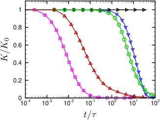
Figure 2: Decaying isotropic turbulence: time evolution of turbulence kinetic energy for rhoEnergyFoam in Mode A (right triangles), Mode B (gradient symbols), Mode C with $\theta^{*}=0$ (deltas), and for dnsFOAM (circles), rhoCentralFoam (squares). $\tau$ is the eddy turnover time.

In order to quantify the energy preservation properties of the present solver, numerical simulations of decaying homogeneous isotropic turbulence are carried out at zero physical viscosity. Random initial conditions are used with prescribed energy spectrum [37],

$$E(k)=16\sqrt{\frac{2}{\pi}}\frac{u_{0}^{2}}{k_{0}}\left(\frac{k}{k_{0}}\right)^{4}e^{-2(k/k_{0})^{2}},$$ (11)

where $k_{0}=4$ is the most energetic mode, and $u_{0}$ is the initial r.m.s. velocity. The initial turbulent Mach number is $M_{t0}=\sqrt{3}u_{0}/c_{0}=0.01$ ($c_{0}$ is the initial mean sound speed), and time is made nondimensional with respect to the eddy turnover time $\tau=2\sqrt{3}/(k_{0}M_{t0}c_{0})$. Numerical simulations are carried out on a $32^{3}$ Cartesian mesh with spacing $\Delta x$, and the time step $\Delta t$ is kept constant, corresponding to an initial Courant number $\mathrm{CFL}=\max{(u_{0}+c_{0})}{\Delta t}/{\Delta x}=1$. Figure 2 shows the turbulence kinetic energy $K=1/2\sum_{i}\overline{u_{i}u_{i}}V_{i}$, as a function of time for rhoEnergyFoam in the three modes of operation previously described. Note that in the numerical experiments the threshold for activation of the convective diffusive fluxes is here momentarily set to zero, to give a perception for the maximum possible amount of numerical diffusion in shock-capturing simulations. For comparison purposes, results obtained with rhoCentralFoam and with the OpenFOAM^® incompressible DNS solver (dnsFoam) are also shown. It is clear that both baseline OpenFOAM^® solvers are not capable of preserving the total kinetic energy, because of the presence of numerical diffusion, which is higher in rhoCentralFoam. As expected, total kinetic energy is exactly preserved from rhoEnergyFoam when operated in Mode A. The addition of numerical diffusion to the pressure term (Mode B) causes some numerical diffusion, although still smaller than dnsFoam, and most kinetic energy is in fact retained for one eddy turn-over time. Operation in Mode C (with $\theta^{*}=0$) further increases numerical diffusion, although the behavior is still sensibly better than rhoCentralFoam.

3.2 Taylor-Green flow

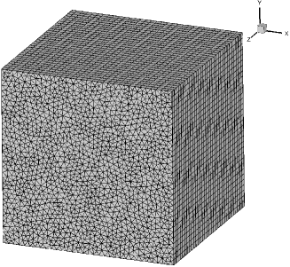
Figure 3: Unstructured mesh for numerical simulation of Taylor-Green flow.

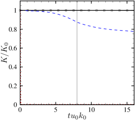
(a)    (b)

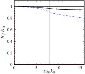
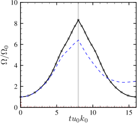
(c)    (d)

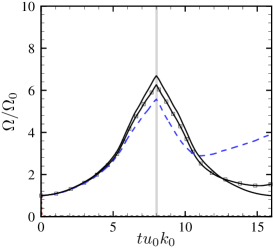
Figure 4: Time evolution of total kinetic energy (a-b), and enstrophy (c-d) for Taylor-Green flow at $M_{0}=0.01$ on Cartesian mesh (a-c) and on unstructured mesh (b-d). Data are shown for rhoEnergyFoam in Mode A (solid lines), rhoEnergyFoam in Mode B (solid lines with square symbols), dnsFoam (dashed lines), and rhoCentralFoam (dotted lines). The vertical line indicates the time $tu_{0}k_{0}=8$, at which velocity vectors are reversed.

The energy-preserving properties of the solver are further tested for the case proposed by Duponcheel et al. [38], namely the time reversibility of the inviscid Taylor-Green flow. The solution is computed in a $(2\pi)^{3}$ triply-periodic box, and initialized as follows

$$\rho =\rho_{0},$$ (12a)

$$u =u_{0}\sin{(k_{0}\,x)}\cos{(k_{0}\,y)}\cos{(k_{0}\,z)},$$ (12b)

$$v =u_{0}\cos{(k_{0}\,x)}\sin{(k_{0}\,y)}\cos{(k_{0}\,z)},$$ (12c)

$$w =0,$$ (12d)

$$p =p_{0}+u_{0}^{2}/16[\cos{(2\,k_{0}\,z)}+2\,(\cos{(2\,k_{0}\,x)}+\cos{(2\,k_{0}\,y)})-2],$$ (12e)

where $k_{0}=1$ is the initial wavenumber, $u_{0}=M_{0}c_{0}$ is the reference velocity (here $M_{0}=0.01$), and $c_{0},p_{0}$, $T_{0}$, and $\rho_{0}$ are the reference speed of sound, pressure, temperature and density. The Taylor-Green flow is widely studied as a model for turbulence formation from ordered initial conditions, exhibiting rapid formation of small-scale structures with incurred growth of vorticity. This flow case is computed both on a Cartesian and an unstructured mesh. The Cartesian mesh has $32^{3}$ cells, whereas the unstructured mesh is obtained by extruding a two-dimensional mesh with triangular cells (see Fig. 3), hence including 85056 triangular prisms. This setting guarantees exact geometrical correspondence of the elements on opposite faces of the computational box, hence periodicity can be exploited in all space directions. The solution is advanced in time up to time $tu_{0}k_{0}=8$, at which all velocity vectors are reversed, and then further advanced in time up to $tu_{0}k_{0}=16$. Based on the mathematical properties of the Euler equations, the initial conditions should be exactly recovered [38].

Numerical diffusion generally spoils time reversibility, as shown in Fig. 4 where we report the time evolution of turbulence kinetic energy and of the total enstrophy, defined as $\Omega=1/2\sum_{i}\overline{\omega_{i}\omega_{i}}V_{i}$. The total kinetic energy (panels a, b) in fact shows monotonic decrease for dnsFoam both on structured and unstructured meshes, and rhoCentralFoam exhibits sudden dissipation of all kinetic energy, on a time scale which is much less than unity (the lines are barely visible in the chosen representation). On the other hand, kinetic energy is almost perfectly retained by rhoEnergyFoam when operated in Mode A, whereas some effect of numerical diffusion is found in Mode B. The total enstrophy computed on a Cartesian mesh (panel c) shows substantial growth up to time reversal, followed by corresponding decrease. However, recovery of the initial condition is imperfect for dnsFoam, and the maximum vorticity at the end of the simulation is higher than expected. This odd behavior is associated with the flow randomization at the end of the forward run, which is not fully recovered in simulations contaminated by numerical diffusion. On unstructured mesh (panel d) the behavior is similar, although the peak enstrophy is lower because of errors associated with mesh distortion. Overall, this test shows that rhoEnergyFoam retains good low-diffusive characteristics also on unstructured meshes which are used in practical engineering computations.

3.3 DNS of supersonic turbulent channel flow

Case	$M_{b}$	$\mbox{{Re}}_{b}$	$\mbox{{Re}}_{\tau}$	$N_{x}$	$N_{y}$	$N_{z}$	$\Delta x^{+}$	$\Delta y_{w}^{+}$	$\Delta z^{+}$	$C_{f}$	$-B_{q}$
CH15-OF	1.5	6000	220	384	128	192	7.20	0.40	4.80	0.0078	0.049
CH15-FD	1.5	6000	220	256	128	192	10.8	0.70	4.80	0.0077	0.048

Table 2: Flow parameters for DNS of plane channel flow for rhoEnergyFoam in Mode A (CH15-OF) and for finite-difference solver [39] (CH15-FD). $M_{b}=u_{b}/c_{w}$ and $\mbox{{Re}}_{b}=2h\rho_{b}u_{b}/\mu_{w}$ are the bulk Mach and Reynolds number, respectively. The computational box is $4\pi h\times 2h\times 4/3\pi$, with $h$ the channel half-height. $N_{i}$ are the mesh points in each coordinate direction, and $\Delta y_{w}^{+}$ is the distance of the first grid point from the wall, $\Delta x^{+}$, $\Delta z^{+}$ are the streamwise and spanwise grid spacings, in wall units. $B_{q}=q_{w}/(\rho_{w}c_{p}u_{\tau}T_{w})$ is the heat flux coefficient and $C_{f}=2\tau_{w}/(\rho_{b}u_{b})$ is the skin friction coefficient.

(a)    (b)

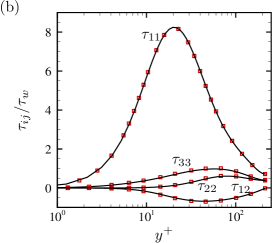
Figure 5: DNS of turbulent flow in plane channel: distribution of mean velocity (a) and Reynolds stresses (b) in wall units for CH15-OF (solid lines) and CH15-FD (squares), for the DNS listed in Tab. 2.

In order to test rhoEnergyFoam for fully resolved compressible turbulent flows we carry out DNS of supersonic channel flow at bulk Mach number $M_{b}=u_{b}/c_{w}=1.5$, and bulk Reynolds number $\mbox{{Re}}_{b}=2h\rho_{b}u_{b}/\mu_{w}=6000$, where $u_{b}$ and $\rho_{b}$ are the bulk channel velocity and density, $c_{w}$ is the speed of sound evaluated at the wall, and $h$ is the channel-half width. Supersonic channel flow is a common prototype of compressible wall-bounded turbulence, and several database have been developed, spanning a wide range of Reynolds numbers [40, 41, 39]. In this flow case a Cartesian mesh is used fine enough that no artificial diffusion is needed, hence the solver is operated in Mode A. The results obtained with rhoEnergyFoam are compared with DNS data obtained with a finite-difference sixth-order accurate energy-preserving solver [39] (see Tab. 2). Figure 5 compares the mean velocity and the Reynolds stresses distributions in wall units and Favre density scaling (denoted with tildas), namely friction velocity $u_{\tau}=(\tau_{w}/\rho_{w})^{1/2}$, and viscous length scale $\delta_{v}=\nu_{w}/u_{\tau}$. The excellent agreement provides convincing evidence for the effectiveness of the solver for DNS of compressible turbulent flows.

3.4 RANS and DES of flow past circular cylinder

Case	$M_{\infty}$	$C_{D}$	$-C_{pbase}$	$\mathrm{St}_{0}$	${\Delta t}_{av}u_{\infty}/D$
URANS	0.1	0.28	0.35	-	220
DES	0.1	0.35	0.44	0.31	150
URANS [42]	-	0.40	0.41	0.31	200
LES [42]	-	0.31	0.32	0.35	200
Exp. [43]	-	0.24	0.33	0.22	-

Table 3: Main estimated properties for turbulent flow around circular cylinder. URANS and DES are carried out using rhoEnergyFoam in Mode B, and compared with previous numerical simulations and experimental data. $C_{D}$ and $C_{pbase}$ are the drag coefficient and the base pressure coefficient, respectively, $\mathrm{St_{0}=f_{0}D/u_{0}}$ is the typical Strouhal number, and ${\Delta t}_{av}$ is the time averaging interval.

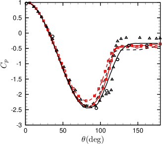
Figure 6: Numerical simulation of flow around circular cylinder: wall pressure coefficient obtained from rhoEnergyFoam in Mode B with URANS (solid line and squares) and DES (dashed line with squares), compared with URANS (solid) and LES (dashed) by Catalano et al. [42] and with experiments by Warschauer and Leene [44] (triangles) and Zdravkovich [45] (circles).

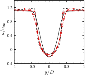
(a)    (b)

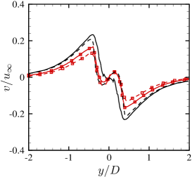
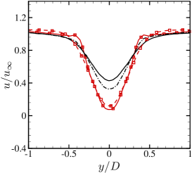
(a)    (b)

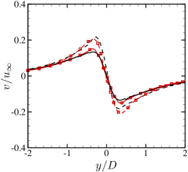
Figure 7: Numerical simulation of flow around circular cylinder: mean velocity profiles at $x/D=0.75$ (a)-(b) and $x/D=1.5$ (c)-(d) for URANS (solid line with squares) and DES (dashed line with squares) compared with URANS (solid) and LES (dashed) by Catalano et al. [42].

The turbulent flow around a circular cylinder is here numerically studied by means of rhoEnergyFoam in mode B, through both unsteady Reynolds-averaged Navier-Stokes simulation (URANS) and detached-eddy simulation (DES), relying on the classical Spalart-Allmaras turbulence model [46] and its DES extension [47], respectively. The free stream Mach number is $M_{\infty}=u_{\infty}/c_{\infty}=0.1$, where $u_{\infty}$ and $c_{\infty}$ are the free stream velocity and speed of sound, and the Reynolds based on the cylinder diameter is $\mbox{{Re}}_{D}=\rho_{\infty}u_{\infty}D/\mu_{w}$, with $\rho_{\infty}$ the free stream density and $\mu_{w}$ the wall viscosity. An O-type mesh is used for DES with $N_{r}\times N_{\theta}\times N_{z}=256\times 256\times 48$ cells in a $L_{r}\times L_{z}=20D\times 2D$ domain, whereas the same mesh with $N_{z}=1$ is used for URANS. The mesh is stretched towards the cylinder with the first off-wall mesh point at $y^{+}\approx 150-200$, hence we rely on the use of wall functions for proper wall-treatment [48]. Specifically, Spalding’s equilibrium law-of-the-wall is used [49]. Isothermal no-slip boundary conditions are imposed at the wall, whereas inlet/outlet boundary conditions are used for all variables at the far field, with the turbulent viscosity set to ${\mu_{t}}_{0}=3\mu_{w}$.

Table 3 shows the flow parameters used for the simulations, as well as the main flow properties including the drag and the base pressure coefficient, and the typical nondimensional frequency in the cylinder wake, as estimated from analysis of the pressure time spectra. The numerical results are compared with previous numerical simulations [42] and experiments [43]. The main difference with respect to those is the absence of sensible vortex shedding in the present URANS, which is probably to be traced to the use of wall functions. Shedding is observed in DES, with global flow parameters in reasonable agreement with other sources. The wall pressure coefficient and the mean velocity profiles in the cylinder wake are further scrutinized in Figs. 6, 7. Comparison is overall satisfactory for both the pressure coefficient and the velocity profiles, with the main difference that a longer cylinder wake is observed both in URANS and DES with respect to the reference numerical simulations of Catalano et al. [42]. Again, this deviation may be ascribed to imprecise prediction of the separation point caused by approximate wall treatment.

3.5 Supersonic flow over forward-facing step

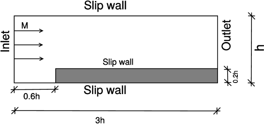
Figure 8: Sketch of the computational setup for flow over a forward-facing step [50].

(a)

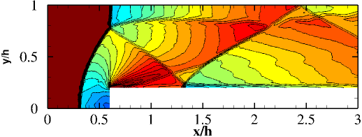
(b)

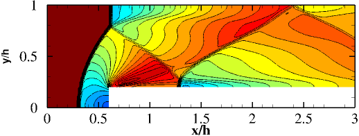
(c)

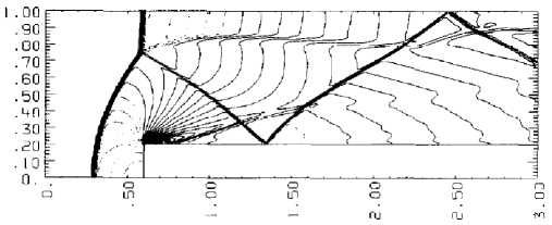
Figure 9: Supersonic flow past forward-facing step at $M_{\infty}=3$. 30 Mach number contours are shown in the range $-0.92\leq\rho\leq 2.86$ (color scale from blue to red) for rhoEnergyFoam (a), rhoCentralFoam (b) and Woodward and Colella [50] (c).

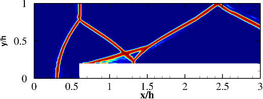
Figure 10: Supersonic flow past forward-facing step at $M_{\infty}=3$: contours of shock sensor, as defined in Eqn. 8. 24 levels are shown in the range $0.05\leq\theta\leq 1$, corresponding to the flow field shown in Fig. 9(a).

The study of the inviscid flow over a forward-facing step was originally proposed by Emery [51] to compare shock-capturing schemes. In particular, we consider the flow configuration used by Woodward and Colella [50], in which the supersonic flow in a channel at $M_{\infty}=3$ faces a step of height $0.2h$, where $h$ is the channel height. The total length of the channel is $3h$, the step leading edge is at $0.6h$ from the inlet and the mesh is uniform, with $N_{x}\times N_{y}=240\times 80$ cells in the coordinate directions (see Fig. 8). Slip boundary conditions are imposed at the top and lower walls, and all variables are extrapolated at the outlet.

For this test case the solver is run in Mode C, with threshold value of the shock sensor $\theta^{*}=0.05$. Fig. 9 shows Mach number contours for rhoEnergyFoam and rhoCentralFoam compared with the reference solution from Woodward and Colella [50]. Inspection of the shock pattern shows that, despite qualitative similarities, rhoEnergyFoam delivers additional flow details which are barely visible with rhoCentralFoam. In particular the slip line issuing from the quadruple point near the top wall in Fig. 9 is evanescent in rhoCentralFoam, because of its higher numerical diffusion. Quantitative differences are also found in the prediction of the Mach stem at the step wall, which is much taller in rhoCentralFoam. Figure 10 shows contours of the shock sensor corresponding to the field shown in Fig. 9(a), which highlights regions in which the convective diffusive flux is activated ($\theta\geq 0.05$). This is a convincing confirmation that numerical diffusion is only activated in close vicinity of shocks.

3.6 Transonic flow over the ONERA M6 wing

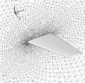
(a)    (b)

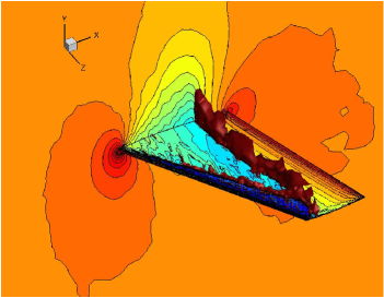
Figure 11: Unstructured mesh around the ONERA M6 wing (a), and computed pressure field with superposed iso-surface of shock sensor ($\theta=0.6$, in red) (b). 32 pressure contours are shown, in the range $0.2\leq p/p_{\infty}\leq 1.3$ (color scale from blue to red).

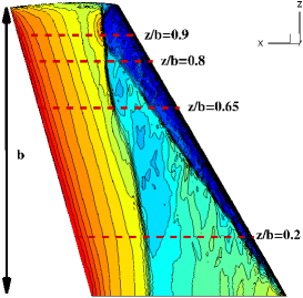
(a)    (b)

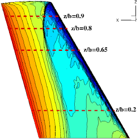
Figure 12: Flow around ONERA M6 wing: computed pressure contours on the wing surface for rhoEnergyFoam (a) and rhoCentralFoam (b). 32 levels are shown in the range $0.3\leq p/p_{\infty}\leq 1.3$ (color scale from blue to red). The dashed lines denote the wing sections used in Fig. 13.

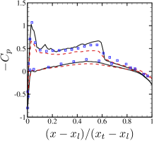
(a)    (b)

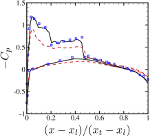
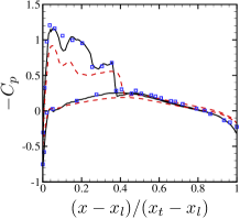
(c)    (d)

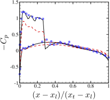
Figure 13: Flow around ONERA M6 wing: pressure coefficient ($C_{p}=(p-p_{\infty})/(1/2\rho_{\infty}u_{\infty}^{2})$) at various wing sections (see Fig. 12): (a) $z/b=0.2$, (b) $z/b=0.65$, (c) $z/b=0.8$, (d) $z/b=0.9$, for rhoEnergyFoam (solid lines) rhoCentralFoam (dashed lines) and experimental data [52] (square symbols). $x_{l}$ and $x_{t}$ denote the coordinates of the leading edge and trailing edge of each wing section, respectively.

Results of numerical simulations of the inviscid flow past the ONERA M6 wing [52] are reported here, at free stream Mach number $M_{\infty}=0.8395$, and angle of attack $\alpha=3.06^{\circ}$. An unstructured mesh including 341797 tetrahedral cells is used (see Fig. 11), within an outer computational box of size $L_{x}\times L_{y}\times L_{z}=10c\times 10c\times 5c$, where $c$ is the chord at the wing root section. Numerical simulations have been carried out using both rhoCentralFoam and rhoEnergyFoam in Mode C, and compared with experimental data. Figure 11b shows the pressure field computed with rhoEnergyFoam with an overlaid iso-surface of the shock sensor, which highlights the presence of two shock waves, a primary one roughly at the middle of the wind chord, and a secondary one close to the leading edge, eventually coalescing near the wing tip.

Figure 12 shows the computed pressure field on the suction surface of the wing for rhoEnergyFoam (panel a) and rhoCentralFoam (panel b), which highlights qualitative differences between the two solvers. Although the main flow features are captured by both the solvers, it seems that the leading-edge shock is much fainter in rhoCentralFoam, and the primary shock is much thicker especially towards the wing root, owing to the diffusive nature of the solver. A more quantitative evaluation is carried out in Fig. 13, where we compare the computed distributions of the pressure coefficient with the experimental data of Schmitt and Charpin [52], at the four wing sections indicated with dashed lines in Fig. 12. At the innermost section (panel a) the primary shock is is rather weak, and barely apparent in rhoCentralFoam, whereas rhoEnergyFoam yields favourable prediction of both shock strength and position. At intermediate sections (panels b,c) both shocks are present, which are again correctly captured by rhoEnergyFoam, whereas rhoCentralFoam shows excessive smearing. At the outermost section (panel d) the primary and the secondary shock merge into a single stronger shock, whose amplitude is well captured by rhoEnergyFoam.

3.7 Transonic flow over the RAE-2822 airfoil

Case	$C_{l}$	$C_{d}$
rhoEnergyFoam	0.713	0.0133
rhoCentralFoam	0.725	0.0185
Experiment [53]	0.743	0.0127

Table 4: Lift and drag coefficient of RAE 2822 airfoil at $M_{\infty}=0.725$, $\mbox{{Re}}_{c}=6.5\times 10^{6}$, $\alpha=2.31^{\circ}$, as predicted by rhoEnergyFoam and rhoCentralFoam, compared with experimental data [53].

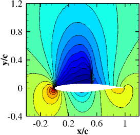
(a)    (b)

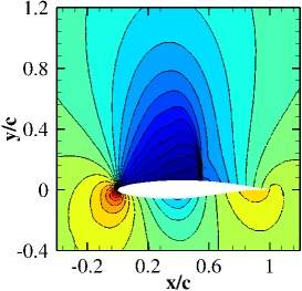
Figure 14: RANS of flow over RAE 2822 airfoil: computed pressure field as predicted by rhoEnergyFoam (a) and rhoCentralFoam (b). 24 contour levels are shown in the range $0.6\leq p/p_{\infty}\leq 1.4$, in color scale from blue to red.

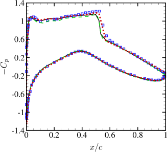
Figure 15: RANS of flow over RAE 2822 airfoil: pressure coefficient predicted by rhoEnergyFoam (solid lines), rhoCentralFoam (dots), compared with previous RANS [54] (dashed lines) and experimental data [53] (square symbols).

The transonic flow past RAE 2822 airfoil [54] has been simulated through RANS, using the standard Spalart-Allmaras model. The flow conditions corresponds to those of test case 6 in the experiments of Cook et al. [53], namely free stream Mach number $M_{\infty}=0.729$, chord Reynolds number $\mbox{{Re}}_{c}=\rho_{\infty}u_{\infty}c/\mu_{\infty}=6.5\times 10^{6}$, and angle of attack $\alpha=2.31^{\circ}$. A C-type structured mesh is used which includes $369\times 256$ cells. The far field boundary is at approximately $20$ chords from the wall, where inlet/outlet boundary conditions are enforced, whereas isothermal no-slip boundary conditions are imposed at the airfoil wall. The distance of the first mesh point off the wall ranges between $\Delta_{y}^{+}=25-180$, hence the wall is modeled through Spalding’s wall function. Table 4 shows the lift and drag coefficient predicted by rhoEnergyFoam in Mode C and rhoCentralFoam, as compared with experimental data [53]. The agreement is quite good, with some overestimation of drag from rhoCentralFoam. The computed pressure fields are compared in Fig. 14, which shows the presence of a single normal shock on the suction side, and very minor differences between the two solvers. Detailed comparison of the pressure coefficient with experiments [53] and simulations [54], shown in Fig. 15, is satisfactory for both solvers, although in this case rhoCentralFoam seems to be closer to experiments, and rhoEnergyFoam closer to previous simulations.

4 Conclusions

A novel numerical strategy has been proposed for accurate simulation of smooth and shocked compressible flows in the context of industrial applications. The algorithm relies on the use of an underlying energy-consistent, non-diffusive numerical scheme, which is locally augmented with the diffusive numerical flux of the AUSM scheme, in an amount dependent on the local smoothness of the flow on the computational mesh. Three modes of solver operation have been suggested, based on the intent of the simulation. We have found that fully resolved simulations (i.e. DNS) can be handled with no numerical diffusion (Mode A). Smooth unresolved flows (i.e. DES and RANS) require some small amount of numerical diffusion, granted by the pressure diffusive flux of AUSM (Mode B). Shocked flows require further addition of the convective diffusive flux of AUSM for stability (Mode C). For the sake of showing simplicity and generality of the approach, the method has been implemented in the OpenFOAM^® library. A broad range of academic-to-applicative test cases have been presented to highlight the main features of the solver. The simulation of homogeneous isotropic turbulence and Taylor-Green flow show that the solver operated in Mode A is capable of discretely preserving the discrete total kinetic energy from convection in the inviscid limit, whereas the baseline version of the OpenFOAM^® solvers herein tested cannot. This features, besides being essential for DNS, is also appealing for URANS and DES. The applicative test cases here presented in fact support the statement that the use of low-diffusive numerics yields better representation of the flow physics, in contrast to highly diffusive schemes which tends to blur many features of the flow field. This is reflected in improved quantitative prediction of local and global force coefficients in applied aerodynamics test cases.

Acknowledgements
We acknowledge that the numerical simulations reported in this paper have been carried out on the Galileo cluster based at CINECA, Casalecchio di Reno, Italy, using resources from the SHAPE project.

5 Appendix

Referring to Fig. 1, the AUSM convective and pressure flux to be used in Eqn. (5) are given below, based on the AUSM⁺-up formulation [55]

$$\hat{\mathbf{f}}_{ON}^{AUSM}=-\frac{c_{ON}}{2}\left[\left(\frac{1}{2}\delta m_{ON}-|M_{ON}|\right)\boldsymbol{\varphi}_{L}+\left(\frac{1}{2}\delta m_{ON}+|M_{ON}|\right)\boldsymbol{\varphi}_{R}\right],$$ (13)

$$\hat{\mathbf{p}}_{ON}^{AUSM}=-\frac{1}{2}\delta\mathbf{p}_{ON},$$ (14)

$$M_{ON}=\frac{M_{R}+M_{L}}{2}-\frac{1}{2}\delta m_{ON}+M_{p},$$ (15)

$$\delta m_{ON}=\left[\Delta\mathcal{M}(M_{R})-\Delta\mathcal{M}(M_{L})\right],\quad\Delta\mathcal{M}(M)=\mathcal{M}_{(4)}^{+}(M)-\mathcal{M}_{(4)}^{-}(M),$$ (16)

$$M_{p}=-\frac{k_{p}}{f_{a}}\max{(1-\sigma\overline{M}^{2},0)}\,\frac{2\,(p_{R}-p_{L})}{(\rho_{L}+\rho_{R})c_{ON}^{2}}.$$ (17)

The speed of sound at the cell interface is evaluated as $c_{ON}=(c_{L}+c_{R})/2$ and $\overline{M}^{2}=\left({u_{n}}_{L}^{2}+{u_{n}}_{R}^{2}\right)/(2c_{ON}^{2})$, $M_{0}^{2}=\min{(1,\max{(\overline{M}^{2},M_{\infty}^{2})})}$, $f_{a}(M_{0})=M_{0}(2-M_{0})$, with $k_{p}=0.25$, $k_{u}=0.75$, $\sigma=1$. The diffusive pressure flux is given by

$$\delta p_{ON}=\left[p_{R}\Delta\mathcal{P}(M_{R})-p_{L}\Delta\mathcal{P}(M_{L})\right]-2M_{u},\quad\Delta\mathcal{P}(M)=\mathcal{P}_{(5)}^{+}(M)-\mathcal{P}_{(5)}^{-}(M),$$ (18)

where

$$M_{u}=-\frac{1}{2}k_{u}\mathcal{P}^{+}_{(5)}(M_{L})\mathcal{P}^{-}_{(5)}(M_{R})\left(\rho_{L}+\rho_{R}\right)\left(f_{a}c_{ON}\right)\left({u_{n}}_{R}-{u_{n}}_{L}\right),$$ (19)

The subscript $L,R$ refers to the two sides of the cell interface, which have have been reconstructed through the Minmod limiter, also available in the OpenFOAM^® library. We further define the split Mach numbers $\mathcal{M}_{(m)}$ as $m$-th degree polynomials

$$\mathcal{M}^{\pm}_{(1)}(M)=\frac{1}{2}\left(M\pm|M|\right),$$ (20)

$$\mathcal{M}^{\pm}_{(2)}(M)=\pm\frac{1}{4}\left(M\pm 1\right)^{2},$$ (21)

$$\mathcal{M}^{\pm}_{(4)}(M)=\begin{cases}\mathcal{M}^{\pm}_{(1)}(M)&if\,\,\,|M|\geq 1\\ \mathcal{M}_{(2)}^{\pm}(M)\left(1\mp 16\beta\mathcal{M}^{\mp}_{(1)}(M)\right)&if\,\,\,|M|<1.\end{cases}$$ (22)

$\mathcal{P}^{\pm}_{(5)}$ is also defined in terms of the split Mach numbers, as follows

$$\mathcal{P}^{\pm}_{(5)}(M)=\begin{cases}\frac{1}{M}\mathcal{M}_{(1)}^{\pm}(M)&if\quad|M|\geq 1\\ \mathcal{M}_{(2)}^{\pm}(M)\left[\left(2\pm-M\right)\mp 16\alpha M\mathcal{M}_{(2)}^{\mp}(M)\mathcal{M}_{(1)}^{\pm}(M)\right]&if\quad|M|<1.\end{cases}$$ (23)

Following Liou [55], we set $\alpha=3/16(-4+5f_{a}^{2})$, $\beta=1/8$.

References

- Orszag and Patterson [1972] S. Orszag, G. Patterson, Numerical simulation of three-dimensional homogeneous isotropic turbulence, Phys. Rev. Lett. 28 (1972) 76.
- Kim et al. [1987] J. Kim, P. Moin, R. Moser, Turbulence statistics in fully developed channel flow at low Reynolds number, J. Fluid Mech 177 (1987) 133–166.
- Schlatter and Örlü [2010] P. Schlatter, R. Örlü, Assessment of direct numerical simulation data of turbulent boundary layers, J. Fluid Mech. 659 (2010) 116–126.
- Sillero et al. [2013] J. Sillero, J. Jiménez, R. Moser, One-point statistics for turbulent wall-bounded flows at Reynolds numbers up to 2000, Phys. Fluids (1994-present) 25 (2013) 105102.
- Bernardini et al. [2014] M. Bernardini, S. Pirozzoli, P. Orlandi, Velocity statistics in turbulent channel flow up to R, J. Fluid Mech. 742 (2014) 171–191.
- Kim et al. [1999] S. Kim, D. Choudhury, B. Patel, Computations of complex turbulent flows using the commercial code FLUENT, in: Modeling complex turbulent flows, Springer, 1999, pp. 259–276.
- Iaccarino [2001] G. Iaccarino, Predictions of a turbulent separated flow using commercial CFD codes, J. Fluids Eng. 123 (2001) 819–828.
- Mahesh et al. [2006] K. Mahesh, G. Constantinescu, S. Apte, G. Iaccarino, F. Ham, P. Moin, Large-eddy simulation of reacting turbulent flows in complex geometries, J. Appl. Mech. 73 (2006) 374–381.
- Bernardini et al. [2016] M. Bernardini, D. Modesti, S. Pirozzoli, On the suitability of the immersed boundary method for the simulation of high-Reynolds-number separated turbulent flows, Computers & Fluids 130 (2016) 84–93.
- Hussaini and Zang [1987] M. Hussaini, T. Zang, Spectral methods in fluid dynamics, Annu. Rev. Fluid Mech. 19 (1987) 339–367.
- Lele [1992] S. Lele, Compact finite difference schemes with spectral-like resolution, J. Comput. Phys. 103 (1992) 16–42.
- Harlow and Welch [1965] F. Harlow, J. Welch, Numerical calculation of time-dependent viscous incompressible flow of fluid with free surface, Phys. Fluids 8 (1965) 2182.
- Orlandi [2012] P. Orlandi, Fluid flow phenomena: a numerical toolkit, volume 55, Springer Science & Business Media, 2012.
- Jameson et al. [1981] A. Jameson, W. Schmidt, E. Turkel, Numerical solutions of the euler equations by finite volume methods using Runge-Kutta time-stepping schemes, AIAA Paper 12-59 (1981) 1981.
- Suresh and Huynh [1997] A. Suresh, H. Huynh, Accurate monotonicity-preserving schemes with Runge-Kutta time stepping, J. Comput. Phys. 136 (1997) 83–99.
- Pirozzoli [2002] S. Pirozzoli, Conservative hybrid compact-WENO schemes for shock-turbulence interaction, J. Comput. Phys. 178 (2002) 81–117.
- Pirozzoli [2011] S. Pirozzoli, Numerical methods for high-speed flows, Annu. Rev. Fluid Mech. 43 (2011) 163–194.
- Hickel et al. [2014] S. Hickel, C. Egerer, J. Larsson, Subgrid-scale modeling for implicit large eddy simulation of compressible flows and shock-turbulence interaction, Phys. Fluids (1994-present) 26 (2014) 106101.
- Patankar and Spalding [1972] S. Patankar, D. Spalding, A calculation procedure for heat, mass and momentum transfer in three-dimensional parabolic flows, Int. J. Heat Mass Transf. 15 (1972) 1787–1806.
- Ferziger and Peric [2012] J. Ferziger, M. Peric, Computational methods for fluid dynamics, Springer Science & Business Media, 2012.
- Mittal and Moin [1997] R. Mittal, P. Moin, Suitability of upwind-biased finite difference schemes for large-eddy simulation of turbulent flows, AIAA J. 35 (1997) 1415–1417.
- Nicolaides and Wu [1997] R. Nicolaides, X. Wu, Covolume solutions of three-dimensional div-curl equations, SIAM J. Numer. Anal. 34 (1997) 2195–2203.
- Ducros et al. [2000] F. Ducros, F. Laporte, T. Souleres, V. Guinot, P. Moinat, B. Caruelle, High-order fluxes for conservative skew-symmetric-like schemes in structured meshes: application to compressible flows, J. Comput. Phys. 161 (2000) 114–139.
- Perot [2000] B. Perot, Conservation properties of unstructured staggered mesh schemes, J. Comput. Phys. 159 (2000) 58–89.
- Weller et al. [1998] H. Weller, G. T. Hrvoje, C. Fureby, A tensorial approach to computational continuum mechanics using object-oriented techniques, Comput. Phys. 12 (1998) 620–631.
- Kurganov and Tadmor [2000] A. Kurganov, E. Tadmor, New high-resolution central schemes for nonlinear conservation laws and convection-diffusion equations, J. Comput. Phys. 160 (2000) 241–282.
- Vuorinen et al. [2012] V. Vuorinen, M. Larmi, P. Schlatter, L. Fuchs, B. Boersma, A low-dissipative, scale-selective discretization scheme for the Navier-Stokes equations, Comput. Fluids 70 (2012) 195–205.
- Vuorinen et al. [2014] V. Vuorinen, J. Keskinen, C. Duwig, B. Boersma, On the implementation of low-dissipative Runge-Kutta projection methods for time dependent flows using OpenFOAM®, Comput. Fluids 93 (2014) 153–163.
- Shen et al. [2014] C. Shen, F. Sun, X. Xia, Implementation of density-based solver for all speeds in the framework of openFOAM, Comput. Phys. Commun. 185 (2014) 2730–2741.
- Shen et al. [2016] C. Shen, X.-L. Xia, Y.-Z. Wang, F. Yu, Z.-W. Jiao, Implementation of density-based implicit lu-sgs solver in the framework of OpenFOAM, Adv. Eng. Softw. 91 (2016) 80–88.
- Liou et al. [1993] M. Liou, , C. Steffen, A new flux splitting scheme, J. Comput. Phys. 107 (1993) 23–39.
- Cerminara et al. [2016] M. Cerminara, T. E. Ongaro, L. Berselli, ASHEE-1.0: a compressible, equilibrium-Eulerian model for volcanic ash plumes, Geosci. Model Dev. 9 (2016) 697–730.
- Pirozzoli [2010] S. Pirozzoli, Generalized conservative approximations of split convective derivative operators, J. Comput Phys. 229 (2010) 7180–7190.
- Pirozzoli [2011] S. Pirozzoli, Stabilized non-dissipative approximations of Euler equations in generalized curvilinear coordinates, J. Comput. Phys. 230 (2011) 2997–3014.
- Ducros et al. [1999] F. Ducros, V. Ferrand, F. Nicoud, C. Weber, D. Darracq, D. Gacherieu, T. Poinsot, Large-eddy simulation of the shock/turbulence interaction, J. Comput. Phys. 152 (1999) 517–549.
- Hirsch [2007] C. Hirsch, Numerical computation of internal and external flows: The fundamentals of computational fluid dynamics, Butterworth-Heinemann, 2007.
- Blaisdell et al. [1991] G. Blaisdell, N. Mansour, W. Reynolds, Numerical simulation of compressible homogeneous turbulence, Report TF-50, Thermosciences Division,Dep. Mech. Eng., Stanford University, 1991.
- Duponcheel et al. [2008] M. Duponcheel, P. Orlandi, G. Winckelmans, Time-reversibility of the Euler equations as a benchmark for energy conserving schemes, J. Comput. Phys. 227 (2008) 8736–8752.
- Modesti and Pirozzoli [2016] D. Modesti, S. Pirozzoli, Reynolds and Mach number effects in compressible turbulent channel flow, Int. J. Heat Fluid Flow 59 (2016) 33–49.
- Coleman et al. [1995] G. Coleman, J. Kim, R. Moser, A numerical study of turbulent supersonic isothermal-wall channel flow, J. Fluid Mech. 305 (1995) 159–183.
- Lechner et al. [2001] R. Lechner, J. Sesterhenn, R. Friedrich, Turbulent supersonic channel flow, J. Turbul. 2 (2001) 1–25.
- Catalano et al. [2003] P. Catalano, M. Wang, G. Iaccarino, P. Moin, Numerical simulation of the flow around a circular cylinder at high Reynolds numbers, Int. J. Heat Fluid Flow 24 (2003) 463–469.
- Shih et al. [1993] W. Shih, C. Wang, D. Coles, A. Roshko, Experiments on flow past rough circular cylinders at large Reynolds numbers, J. Wind Eng. Indust. Aerodyn. 49 (1993) 351–368.
- Warschauer and Leene [1971] K. Warschauer, J. Leene, Experiments on mean and fluctuating pressures of circular cylinders at cross flow at very high Reynolds numbers, in: Proc. Int. Conf. on Wind Effects on Buildings and Structures, pp. 305–315.
- Zdravkovich [1997] M. Zdravkovich, Flow around circular cylinders. Fundamentals, Vol. 1, 1997.
- Spalart and Allmaras [1992] P. Spalart, S. Allmaras, A one equation turbulence model for aerodinamic flows., AIAA J. 94 (1992) 6–10.
- Spalart et al. [1997] P. Spalart, W. Jou, M. Strelets, S. Allmaras, Comments on the feasibility of LES for wings, and on a hybrid RANS/LES approach, Advances in DNS/LES 1 (1997) 4–8.
- Piomelli and Balaras [2002] U. Piomelli, E. Balaras, Wall-layer models for large-eddy-simulations, Annu. Rev. Fluid Mech. 34 (2002) 349–374.
- Spalding [1961] D. Spalding, A single formula for the ”law of the wall”, J. Appl. Mech. 28 (1961) 455–458.
- Woodward and Colella [1984] P. Woodward, P. Colella, The numerical simulation of two-dimensional fluid flow with strong shocks, J. Comput. Phys. 54 (1984) 115–173.
- Emery [1968] A. Emery, An evaluation of several differencing methods for inviscid fluid flow problems, J. Comput. Phys. 2 (1968) 306–331.
- Schmitt and Charpin [1979] V. Schmitt, F. Charpin, Pressure distributions on the ONERA-M6-wing at transonic Mach numbers, AGARD Advisory Report, AR-138, 1979.
- Cook et al. [1979] P. Cook, M. Firmin, M. McDonald, Aerofoil RAE 2822: pressure distributions, and boundary layer and wake measurements, AGARD Advisory Report, AR-138, 1979.
- Nelson and Dudek [2009] C. Nelson, J. Dudek, RAE 2822 Transonic Airfoil: Study 5, 2009.
- Liou [2006] M. Liou, A sequel to AUSM, Part II: AUSM+-up for all speeds, J. Comput. Phys. 214 (2006) 137–170.