Three-dimensional Topological Insulators

and Bosonization

Andrea CAPPELLI^(a),   Enrico RANDELLINI^(a,b),    Jacopo SISTI^(c)

^(a) INFN, Sezione di Firenze
^(b) Dipartimento di Fisica e Astronomia, Università di Firenze
Via G. Sansone 1, 50019 Sesto Fiorentino - Firenze, Italy

^(c) SISSA, Via Bonomea 265, 34136 Trieste, Italy

Massless excitations at the surface of three-dimensional time-reversal invariant topological insulators possess both fermionic and bosonic descriptions, originating from band theory and hydrodynamic BF gauge theory, respectively. We analyze the corresponding field theories of the Dirac fermion and compactified boson and compute their partition functions on the three-dimensional torus geometry. We then find some non-dynamic exact properties of bosonization in $(2+1)$ dimensions, regarding fermion parity and spin sectors. Using these results, we extend the Fu-Kane-Mele stability argument to fractional topological insulators in three dimensions.

1 Introduction

The topological phases of matter [1, 2, 3, 4] have been described by several approaches, such as wavefunction modeling [5], band theory [6] and effective field theory of boundary excitations [7, 8], whose interplay has been extremely rich and fruitful. In this paper, we analyze $(3+1)$-dimensional time-reversal invariant topological insulators using field theory methods.

The main motivation of our study is the success of the field theory approach for $(2+1)$ dimensional topological states, where exact methods are available for describing the one-dimensional edge excitations, most notably those of conformal field theory [9]. In several instances, these methods give access to strongly interacting dynamics and make use of powerful symmetry principles. The extensive modeling of quantum Hall states has been applied to the description of the quantum spin Hall effect and then to time-reversal invariant topological insulators [10].

In particular, the $\mathbb{Z}_{2}$ characterization of stability of topological insulators, originally derived within band theory by Fu, Kane and Mele [11, 12], has been reformulated in field-theory language and extended to interacting fermion models with Abelian [10] and non-Abelian [13, 14] fractional statics of excitations. The $\mathbb{Z}_{2}$ stability also extends to $(3+1)$ dimensional band insulators and it is interesting to find the corresponding field theory argument for analyzing interacting systems. In this paper, we shall present results in this direction.

More generally, the theoretical methods in $(3+1)$ dimensions are facing the problem of bosonization, namely that of finding correspondences between two seemingly different theoretical approaches:

• That of fermionic theories, dealing with band structures and topological effects related to Berry phases, and leading to the ten-fold classification of non-interacting topological states [6].

• That of bosonic theories, also called hydrodynamic approach, dealing with topological gauge theories and their description of braiding relations and boundary excitations [15, 16, 8, 17, 18].

Bosonization is an exact map in $(1+1)$-dimensional field theories that is very well understood [9]; thus, the above interplay does not cause any problem for $(2+1)$-dimensional topological states. The bosonic approach can provide exact results for interacting systems and well as the methods for discussing bulk wavefunctions and braiding statistics.

In this paper, we review and develop both the fermionic and bosonic field theory descriptions of massless surface states for time-reversal invariant topological insulators in $(3+1)$ dimensions. Our main method is the study of partition functions on the space-time geometry of the three-torus and their behaviour under flux insertions and modular transformations, namely for large gauge transformations of the electromagnetic and gravitational backgrounds [19, 13]. In the fermionic theory, we study the free Dirac excitations at the surface of topological insulators [20]. In the bosonic approach, we analyze the BF topological theory and the associated bosonic field theory of surface excitations [8, 21]. We then quantize the theory of the compactified boson.

Although these fermionic and bosonic theories are different in $(2+1)$ dimensions, we can establish some basic properties of bosonization that are exact being independent of dynamics:

• We show that the quantization of the compactified boson in $(2+1)$ dimension yields eight sectors that correspond to the spin sectors of the fermionic theory on the three-torus. The partition functions in the two theories transform in the same way under flux insertions and modular transformations; actually, they become equal under dimensional reduction to $(1+1)$ dimensions, where bosonization is an exact map.

• We identify the fermion parity of bosonic states and using this assignment we formulate the Fu-Kane-Mele stability argument in the bosonic theory.

• We then prove the stability of interacting topological insulators described by the hydrodynamic BF theory with odd integer coupling constant $K$, possessing fractional changed quasiparticles and fractional Abelian braiding between quasiparticles and vortices.

The paper includes the following parts. In Section 2, we recall the fermionic theory of surface states of topological insulators, compute the partition function on the three-torus and study its transformations properties. We reformulate the Fu-Kane-Mele stability analysis in terms of properties of the spectrum in the different spin sectors and study the dimensional reduction to the two-torus. In section 3, we review the hydrodynamic approach of the BF theory, derive the bosonic surface theory and discuss two Hamiltonians consistent with the topological data. We then quantize the compactified boson and obtain the partition functions. In Section 4, we find their transformation properties, match the fermionic and bosonic sectors, assign the fermion parity and extend the stability analysis to the bosonic theory.

2 Fermionic topological insulators

2.1 Introduction: surface states and anomaly cancellation

We start by recalling some known features of three-dimensional topological band insulators, involving non-interacting fermions with time reversal invariance [2]. At the microscopic level, the topological states occur for an odd number of level crossings between the valence and conduction bands. Near each crossing a Dirac cone is approximatively present and a massless relativistic fermionic excitation is realized at small energies. Actually, this is a $(2+1)$-dimensional Dirac fermion located at the surface of the system [6, 22].

The low-energy effective field theory description of these topological states is realized by the $(3+1)$-dimensional free Dirac fermion with mass $M$ in the bulk that vanishes at the surface [6, 16]. Let us consider a plane located at $z=0$ separating the bulk of the material ($z<0$) from empty space ($z>0$): we can take the mass profile $M(z)=-M_{0}\tanh(z/\ell)$, where $M_{0}$ is of the order of the bulk gap and $\ell$ of the lattice spacing (see Fig. 1).

The Dirac theory with this mass profile possesses massless fermionic surface excitations that are obtained by the so-called Jackiw-Rebbi dimensional reduction, originally formulated for the polyacetylene chain in $(1+1)$ dimensions [23, 1]. Let us recall the main steps of this argument in the case of reduction from $(3+1)$ to $(2+1)$ dimensions. A convenient basis for the $\gamma$ matrices in $d=(3+1)$ is given by:

$$\gamma^{0}=\left(\begin{matrix}0&\sigma_{3}\\ \sigma_{3}&0\end{matrix}\right),\ \ \gamma^{1}=i\left(\begin{matrix}0&\sigma_{1}\\ \sigma_{1}&0\end{matrix}\right),\ \ \gamma^{2}=i\left(\begin{matrix}0&\sigma_{2}\\ \sigma_{2}&0\end{matrix}\right),\ \ \gamma^{3}=i\left(\begin{matrix}1&0\\ 0&-1\end{matrix}\right),$$ (2.1)

where the $\sigma$’s are the Pauli matrices. The Dirac Hamiltonian takes the form:

$$H=-i\gamma^{0}\gamma^{1}\partial_{x}-i\gamma^{0}\gamma^{2}\partial_{y}-i\gamma^{0}\gamma^{3}\partial_{z}+\gamma^{0}M(z)\equiv H_{xy}+H_{z}.$$ (2.2)

We look for eigenstates of $H$ which are simultaneously zero-energy eigenstates of $H_{z}$, so as to realize the dimensional reduction. We assume the separation of variables,

$$H\psi=E\psi,\qquad\quad\psi=\varphi(z)u(x,y),$$ (2.3)

where $\varphi(z)$ is a function and $u(x,y)$ a spinor, and impose the zero-energy condition for $H_{z}$, i.e.

$$\left(i\partial_{z}+\gamma^{3}M(z)\right)\varphi(z)u(x,y)=0.$$ (2.4)

The solutions to this equation are of the form:

$$\psi_{\pm}=\varphi_{\pm}(z)u_{\pm},\qquad\quad\left(\partial_{z}\pm M(z)\right)\varphi_{\pm}(z)=0\ ,\qquad\quad\gamma^{3}u_{\pm}=\pm iu_{\pm}\ .$$ (2.5)

In this equation, the spinor $u_{\pm}$ has non-vanishing components in the upper/lower two-dimensional subspaces of the representation (2.1). Only one solution of (2.5) is normalizable, given the kink shape in Fig. 1, namely $\varphi_{-}$:

$$\varphi_{-}(z)=\exp\left(\int_{0}^{z}dz^{\prime}~{}M(z^{\prime})\right).$$ (2.6)

The explicit calculation shows that this zero mode is localized at the surface $z=0$ where the mass changes sign.

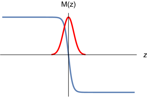
Figure 1: Mass profile $M=M(z)$ (blue line) and wavefunction of the Hamiltonian zero mode (red line).

The remaining surface dynamics is governed by the Hamiltonian $H_{xy}$ acting on spinors of the form $u_{-}=(0,\chi_{-})$, where $\chi_{-}$ is a bicomponent spinor. Once projected in this subspace, $H_{xy}$ takes the form,

$$(k_{y}\sigma_{1}-k_{x}\sigma_{2})\chi_{-}=E\chi_{-}\ ,$$ (2.7)

in terms of surface momenta $(k_{x},k_{y})$. This is the expected Hamiltonian of a massless Dirac excitation in $(2+1)$ dimensions. Of course, the dimensional reduction holds for energies $E\ll M_{0}$.

In a physical setup, the system has two boundaries along the $z$ axis, with the second surface described by the inverted mass profile $M(z)\to-M(z+z_{0})$. Performing the same steps as before, the normalizable zero mode is now given by the positive sign in (2.5), i.e. $u_{+}=(\chi_{+},0)$. It turns out that the bispinor $\chi_{+}$ obeys the same Dirac equation (2.7).

In the study of the microscopic model of band topological insulators, the authors of Ref.[22] considered the expansion of the Hamiltonian for momenta near the band crossing point and obtained the result (2.7) at low-energy. In that approach, the angular momentum of the surface states was also discussed, involving the electron spin as well as a $L=1$ contribution from the $p$-wave orbitals involved. They found that the low-energy surface excitations have angular momentum one-half that is represented by $S_{i}\sim\sigma_{i}$, where the $\sigma_{i}$ are the Pauli matrices introduced before. Therefore, the solutions of (2.7) have associated the values:

$$\langle S_{z}\rangle=0\ ,\qquad\quad\langle S_{x}k_{x}+S_{y}k_{y}\rangle=0\ .$$ (2.8)

Namely, the spin lies on the surface and is orthogonal to momentum (helical spin excitations). These results are in agreement with the time reversal symmetry ${\cal T}$ in $(3+1)$ dimensions: the Dirac mass is ${\cal T}$ invariant, as well as the helical states on the boundary of the topological insulator.

We remark that the analogous Jackiw-Rebbi dimensional reduction from $(2+1)$ to $(1+1)$ dimensions would lead to chiral (resp. antichiral) edge fermions for kink (resp. antikink) mass profile. Indeed, the massive Dirac theory in $(2+1)$ dimensions breaks parity and time reversal symmetries and can model chiral topological states such as the (anomalous) quantum Hall effect and Chern insulators [1]. Analogous Jackiw-Rebbi reductions exist for all ten classes of non-interacting fermionic topological states, and actually provide an independent derivation of the classification [6].

Fermionic surface states with mass $\pm m$ can be introduced by adding the following ${\cal T}$ breaking mass to the $(3+1)$ dimensional Dirac Hamiltonian (2.2):

$$\Delta H=i\gamma^{0}\gamma^{5}m\ .$$ (2.9)

Upon repeating the Jackiw-Rebbi reduction, one find the following $(2+1)$-dimensional Dirac Lagrangians on the two boundary surfaces,

$$\mathcal{L}_{-}=\overline{\chi}_{-}(i\not{\partial}-m)\chi_{-},\qquad\quad\mathcal{L}_{+}=\overline{\chi}_{+}(i\not{\partial}+m)\chi_{+}.$$ (2.10)

Time reversal transformations act as ${\cal T}:m\to-m$; moreover, the two electrons correspond to inequivalent representations of the Clifford algebra, such that the mass sign is physically relevant for surface fermions.

Another result that is relevant for the following discussion is the induced effective action obtained by coupling the $(2+1)$-dimensional fermion to the electromagnetic field $A_{\mu}$. The expansion of the fermionic determinant $\det\left(i\not{\partial}+\not{A}-m\right)$ corresponds to an effective action involving any power of $A_{\mu}$. The first, quadratic term is given by the one-loop vacuum polarization $\Pi_{\mu\nu}$,

$$S_{\rm eff}[A]=-\frac{1}{2}\int\frac{d^{3}k}{(2\pi)^{3}}\ A_{\mu}(k)\Pi_{\mu\nu}(k,m)A_{\nu}(-k)\ +\ O\left(A^{3}\right)\ .$$ (2.11)

This reads in Euclidean space [24, 25]:

$$\Pi_{\mu\nu}(k,m)= \frac{1}{4\pi}k_{\alpha}\epsilon^{\alpha\mu\nu}\left(\frac{m}{|m|}\frac{\arctan(x)}{x}-\frac{\Lambda}{|\Lambda|}\right)$$

$$-\left(k^{2}\delta_{\mu\nu}-k_{\mu}k_{\nu}\right)\frac{1}{8\pi|k|}\left(\frac{1}{x}-\frac{1-x^{2}}{x^{2}}\arctan(x)\right),$$

$$x= \frac{|k|}{2|m|}\ .$$ (2.12)

This expression contains a first term that is odd in momentum, and a second that is even. The first term breaks parity and time reversal, and has been regularized by subtracting the contribution of a Pauli-Villars fermion with mass $\Lambda\to\infty$.

In the limit of large mass $|m|\to\infty$, the expression for $\Pi_{\mu\nu}$ becomes:

$$\Pi_{\mu\nu}(k,m)=\frac{1}{4\pi}k_{\alpha}\epsilon^{\alpha\mu\nu}\left(\frac{m}{|m|}-\frac{\Lambda}{|\Lambda|}\right)-\left(k^{2}\delta_{\mu\nu}-k_{\mu}k_{\nu}\right)\frac{1}{12\pi|m|}\ ,\quad(|m|\gg|k|).$$ (2.13)

The vanishing of the effective action in the static limit fixes the sign of the regulator mass to be ${\rm sign}(\Lambda)={\rm sign}(m)$. In the massless limit, one instead obtains the result

$$\Pi_{\mu\nu}(k,m)=-\frac{1}{4\pi}k_{\alpha}\epsilon^{\alpha\mu\nu}\frac{m}{|m|}-\left(k^{2}\delta_{\mu\nu}-k_{\mu}k_{\nu}\right)\frac{1}{16|k|},\qquad(|m|\ll|k|).$$ (2.14)

The first term corresponds to an induced Chern-Simons action,

$$S_{CS}[A]=i\frac{K}{4\pi}\int d^{3}x\,\varepsilon^{\mu\nu\rho}A_{\mu}\partial_{\nu}A_{\rho},\qquad\quad K=\frac{1}{2}\frac{m}{|m|}\ .$$ (2.15)

Therefore, in the massless theory the parity and time reversal symmetries are restored but are broken at the quantum level: this is the $\mathbb{Z}_{2}$ anomaly of $(2+1)$-dimensional fermions [25]. Note that the sign of Chern-Simons coupling $K$, i.e. the sign of the Pauli-Villars regulator, cannot be determined in the massless theory without referring to a massive phase [26]. The second, parity invariant term in the effective action (2.12) will be relevant for the discussion in Section 3.2.

In the case of topological insulators, the anomaly (2.15) of surface massless states cancels against the bulk contribution. Let us recall how this occurs. The bulk action is given by the Abelian theta term [16],

$$S_{\theta}[A]=-\frac{\theta}{32\pi^{2}}\int d^{4}x~{}\epsilon^{\mu\nu\lambda\rho}F_{\mu\nu}F_{\lambda\rho},$$ (2.16)

with parameter $\theta=\pi$. In the geometry of the slab considered here, $S_{\theta}[A]$ is a total derivative that reduces to the Chern-Simons action (2.15) on the two surfaces with coupling taking opposite values $K=\pm 1/2$.

Furthermore, in the earlier discussion of the Jackiw-Rebbi reduction we argued that the $(3+1)$-dimensional time-reversal breaking mass induces opposite masses on the two surfaces, Eqs. (2.9), (2.10). It is thus natural to expect that in the $m\to 0$ limit, the corresponding anomalies are given by Chern-Simons actions $S_{CS}^{+}[A]$ and $S_{CS}^{-}[A]$ with opposite couplings $K_{-}=1/2$ and $K_{+}=-1/2$. Therefore, the time-reversal breaking terms cancel in the whole system by matching their signs, as follows:

$$S_{\rm tot}[A]=S^{+}_{CS}[A]+S_{\theta}[A]+S^{-}_{CS}[A]=0\ ,\qquad\quad\theta=\pi.$$ (2.17)

This result establishes the bulk-boundary cancellation of the $\mathbb{Z}_{2}$ anomaly in $(3+1)$-dimensional topological insulators [27, 28]. Actually, it should rather be called a boundary-boundary cancellation: the theta term does not imply local effects in the bulk; its role is that of ‘transporting’ the anomalous action $S_{CS}[A]$ from one surface to the other. This result should be contrasted with the mechanism of ‘anomaly inflow’ [29] in the quantum Hall effect in $(2+1)$ dimensions, where the chiral anomaly of the edge, i.e. the non-conservation of charge, is compensated by the classical Hall current in the bulk [1, 30].

In the case of compact $(3+1)$-dimensional manifolds, $S_{\rm tot}[A]=S_{\theta}[A]$ does not vanish, but is proportional to the integral of the second Chern class ${\cal C}_{2}$ of the gauge field, $S_{\theta}[A]=\theta\,{\cal C}_{2}$. Since ${\cal C}_{2}$ is an integer valued topological invariant quantity, the coupling $\theta$ is defined modulo $2\pi$. Therefore, $S_{\rm tot}[A]$ is time reversal invariant due to the equivalence of the values $\theta=\pi$ and $\theta=-\pi$ [16].

Altogether, topological insulators are time reversal invariant topological states of matter. Their stability with respect to interactions and perturbations is not guaranteed and should be checked carefully. If time reversal symmetry is broken they decay into trivial insulators, i.e. they belong to the class of symmetry protected topological states, to be contrasted with other states, such as Chern insulators, that are chiral and stable [3, 31]. Topological insulators are characterized by a $\mathbb{Z}_{2}$ index of stability, that is zero for unstable/trivial insulators and one for stable/topological insulators [11, 12]. At the level of band theory, this index distinguishes the cases of even number of level crossings, that can be smoothly deformed to no crossing, from that of odd crossings, that can be deformed to one crossing. Within the effective theory, we should consider even and odd numbers of Dirac surface fermions [3, 16]. Since a time-reversal invariant quadratic (mass) interaction can be written in terms of two fermion species, it can be used to gap them in pairs, thus remaining with zero or one massless fermion.

In $(2+1)$-dimensional topological insulators, the $\mathbb{Z}_{2}$ index of stability also holds for systems of interacting fermions, including Abelian [10] as well as non-Abelian [13, 14] fractional insulators. Stability in $(3+1)$-dimensional interacting states is not yet fully understood and some results will be presented in the following sections of the paper.

We finally discuss the explicit breaking of time reversal symmetry at the edge, for example due to proximity with a magnetic material [16]. In this case, the surface fermion acquires a mass and its effective action is given by the expression (2.12) with ${\rm sign}(\Lambda)={\rm sign}(m)$. In the low energy limit, $|k|\ll|m|$, the anomalous term vanishes, as shown by (2.13). It follows that the bulk theta term $S_{\theta}[A]$ is not cancelled as in (2.17) and it reduces to (minus) the Chern-Simons action (2.15) at the surface. This implies a surface Hall effect with conductivity $\sigma_{H}=e^{2}\nu/h$, $\nu=1/2$ [32].

2.2 Torus partition functions

In this section, we derive the partition function of the Dirac fermion on the surface of the $(3+1)$-dimensional topological insulator. Extending our earlier analysis in one less dimension [13], we use the partition function to reformulate the Fu-Kane-Mele stability argument for the existence of massless surface states in presence of disorder and interactions that are time reversal invariant (the ‘strong topological insulators’ of Ref.[11]). These results are also the starting point for discussing the stability of bosonic surface states in Section 4.

We consider the spatial geometry of a ‘Corbino donut’ (see Fig. 2), whose internal and external surfaces are two-torii. The space-time three-torus $\mathbb{T}^{3}$ is obtained by considering one boundary and the Euclidean time with period the temperature $T$. The partition functions for periodic $(P)$ and anti-periodic $(A)$ boundary conditions in space and time form a eight-dimensional multiplet, corresponding to the eight spin sectors of $\mathbb{T}^{3}$. Our derivation of the partition functions uses results of Ref.[33][20].

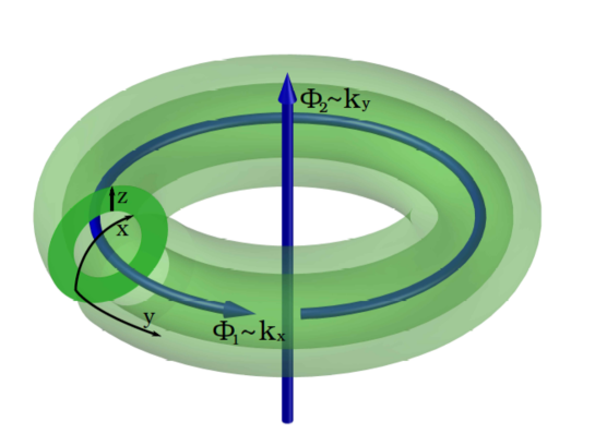
Figure 2: Three-dimensional Corbino donut. The addition of fluxes $\Phi_{1}$ and $\Phi_{2}$ modifies the quantization of $k_{x}$ and $k_{y}$ momenta, respectively.

The $\mathbb{T}^{3}$ torus is defined by the generators of the periodicity lattice $\boldsymbol{\omega}_{\mu},\mu=0,1,2$, (see Fig. 3), whose components form the following matrix:

$$\begin{pmatrix}\boldsymbol{\omega}_{0}\\ \boldsymbol{\omega}_{1}\\ \boldsymbol{\omega}_{2}\end{pmatrix}=\begin{pmatrix}\omega_{00}&\omega_{01}&\omega_{02}\\ 0&\omega_{11}&\omega_{12}\\ 0&\omega_{21}&\omega_{22}\end{pmatrix}\ .$$ (2.18)

The dual vectors $\boldsymbol{k}_{\mu}$ are defined by $\boldsymbol{k}_{\mu}\cdot\boldsymbol{\omega}_{\nu}=\delta_{\mu\nu}$; their spatial components will be indicated as:

$$\vec{\omega}_{i}=(\omega_{1i},\omega_{2i}),\ \ \ \ \ \ \vec{k}_{i}=(k_{1i},k_{2i}),\qquad i=1,2.$$ (2.19)

The volumes $V^{(3)}$ and $V^{(2)}$ of the $3D$ space-time and $2D$ space cells are respectively given by:

$$V^{(3)}=\text{det}(\boldsymbol{\omega}),\ \ \ \ V^{(2)}=\text{det}\ \vec{\omega}=|\boldsymbol{\omega}_{1}\times\boldsymbol{\omega}_{2}|.$$ (2.20)

Some useful relations are:

$$k_{11}=\frac{\omega_{22}}{V^{(2)}},\ \ \ k_{12}=-\frac{\omega_{21}}{V^{(2)}},\ \ \ k_{21}=-\frac{\omega_{12}}{V^{(2)}},\ \ \ k_{22}=\frac{\omega_{11}}{V^{(2)}},\quad\omega_{00}=\frac{V^{(3)}}{|\boldsymbol{\omega}_{1}\times\boldsymbol{\omega}_{2}|}\ .$$ (2.21)

The partition function is given in terms of the on-shell data of the free fermion, namely its spectra of energy, momentum, charge and fermion number. The usual creation and annihilation operators of particles $(a_{\vec{n}}^{\dagger},a_{\vec{n}})$ and antiparticles $(b_{\vec{n}}^{\dagger},b_{\vec{n}})$ , where $\vec{n}=(n_{1},n_{2})\in\mathbb{Z}^{2}$, obey anti-commutation relations and satisfy the vacuum conditions

$$a_{\vec{n}}\ket{\Omega}=b_{\vec{n}}\ket{\Omega}=0\ ,\qquad\quad n_{1},n_{2}\in\mathbb{Z}\ .$$ (2.22)

The energy, momentum, charge and fermion number of excitations are given by the following normal ordered expressions:

$$E=\sum_{\vec{n}}E_{\vec{n}}\left(a^{\dagger}_{\vec{n}}a_{\vec{n}}+b_{\vec{n}}^{\dagger}b_{\vec{n}}-1\right)\ ,\qquad E_{\vec{n}}=2\pi\big{|}(n_{1}+\alpha_{1})\vec{k}_{1}+(n_{2}+\alpha_{2})\vec{k}_{2}\big{|},$$ (2.23)

$$P_{i}=\sum_{\vec{n}}p_{\vec{n}}\left(a^{\dagger}_{\vec{n}}a_{\vec{n}}+b_{\vec{n}}^{\dagger}b_{\vec{n}}\right),\qquad\quad p_{\vec{n}}=2\pi\left((n_{1}+\alpha_{1})k_{1i}+(n_{2}+\alpha_{2})k_{2i}\right),$$ (2.24)

$$Q=\sum_{\vec{n}}a^{\dagger}_{\vec{n}}a_{\vec{n}}-b_{\vec{n}}^{\dagger}b_{\vec{n}},$$ (2.25)

$$(-1)^{F}=(-1)^{\sum_{\vec{n}}a^{\dagger}_{\vec{n}}a_{\vec{n}}+b_{\vec{n}}^{\dagger}b_{\vec{n}}}.$$ (2.26)

In the expression of the energy, the infinite sum $(-\sum_{\vec{n}}E_{\vec{n}})$ to be regularized later yields the Casimir energy and the parameters $\alpha_{i}$ specify the boundary conditions along the $i=1,2$ spatial directions: $\alpha_{i}=0$ (resp. $\alpha_{i}=1/2$) for periodic (P) conditions (resp. anti-periodic (A)) conditions. For convenience, we shall also denote the P (resp. A) conditions in time by using another parameter $\alpha_{0}=0$ (resp. $\alpha_{0}=1/2$).

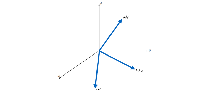
Figure 3: Vector moduli of $\mathbb{T}^{3}$ torus in $(2+1)$ dimensions.

The partition function is evaluated in presence of a scalar potential $A_{0}$ coupling to charge. For $(A)$ boundary conditions in time, it is given by the following expression:

$$Z^{F}_{\frac{1}{2},\alpha_{1}\alpha_{2}}=\text{Tr}\bigg{[}\text{exp}\bigg{(}-T(E+QA_{0})+i\omega_{01}P_{1}+i\omega_{02}P_{2}\bigg{)}\bigg{]}.$$ (2.27)

For $(P)$ boundary conditions in time, the trace includes the operator $(-1)^{F}$:

$$Z^{F}_{0,\alpha_{1}\alpha_{2}}=\text{Tr}\bigg{[}(-1)^{F}\text{exp}\bigg{(}-T(E+QA_{0})+i\omega_{01}P_{1}+i\omega_{02}P_{2}\bigg{)}\bigg{]}.$$ (2.28)

The trace over the fermionic Fock space is straightforward. In the result, we substitute the $\vec{k}_{i}$ vectors in terms of the $\vec{\omega}_{i}$ and introduce the constant $\alpha_{0}=0,1/2$, to obtain:

$$Z^{F}_{\alpha_{0},\alpha_{1}\alpha_{2}} = e^{-V^{(3)}F_{0}}\prod_{n_{1},n_{2}\in\mathbb{Z}}\left\{1-\text{exp}\left(-2\pi\mathcal{E}^{\alpha_{1}\alpha_{2}}_{n_{1}n_{2}}+2\pi i\mathcal{P}^{\alpha_{1}\alpha_{2}}_{n_{1}n_{2}}-2\pi i\mathcal{A}\right)\right\}$$ (2.29)

$$\qquad\qquad\ \ \times\left\{1-\text{exp}\left(-2\pi\mathcal{E}^{\alpha_{1}\alpha_{2}}_{n_{1}n_{2}}-2\pi i\mathcal{P}^{\alpha_{1}\alpha_{2}}_{n_{1}n_{2}}+2\pi i\mathcal{A}\right)\right\}.$$

In this expression,

$$\mathcal{A} = \alpha_{0}-i\frac{V^{(3)}A_{0}}{2\pi|{\boldsymbol{\omega}}_{1}\times{\boldsymbol{\omega}}_{2}|},$$ (2.30)

$$\mathcal{E}^{\alpha_{1}\alpha_{2}}_{n_{1}n_{2}} = \frac{V^{(3)}}{|{\boldsymbol{\omega}}_{1}\times{\boldsymbol{\omega}}_{2}|^{2}}|(n_{1}+\alpha_{1}){\boldsymbol{\omega}}_{2}-(n_{2}+\alpha_{2}){\boldsymbol{\omega}}_{1}|,$$ (2.31)

$$\mathcal{P}^{\alpha_{1}\alpha_{2}}_{n_{1}n_{2}} = \frac{({\boldsymbol{\omega}}_{1}\times{\boldsymbol{\omega}}_{2})}{|{\boldsymbol{\omega}}_{1}\times{\boldsymbol{\omega}}_{2}|^{2}}\left[(n_{1}+\alpha_{1})({\boldsymbol{\omega}}_{0}\times{\boldsymbol{\omega}}_{2})-(n_{2}+\alpha_{2})({\boldsymbol{\omega}}_{0}\times{\boldsymbol{\omega}}_{1})\right],$$ (2.32)

$$F_{0} = \frac{1}{2\pi}\sum_{n_{1},n_{2}}{}^{\prime}~{}\frac{e^{-2\pi i(\alpha_{2}n_{1}-\alpha_{1}n_{2})}}{|n_{1}{\boldsymbol{\omega}}_{2}-n_{2}{\boldsymbol{\omega}}_{1}|^{3}},$$ (2.33)

where $F_{0}$ is the Casimir energy regularized by using Epstein’s analytic continuation formula (see Refs.[33]), with the sum $\sum{}^{\prime}$ excluding the value $(n_{1},n_{2})=(0,0)$.

2.3 Flux insertions and stability argument

The Fu-Kane-Mele argument for stability of time-reversal topological insulators involves three main steps (see Fig. 4 for the two-dimensional case) [11, 10, 13]:

i) First, the ground state of the system is adiabatically deformed by adding half magnetic fluxes, so as to create a neutral spin one-half excitation at the boundary.

ii) Secondly, the Kramers theorem is invoked, saying that this excitation is part of a doublet that remains degenerate in presence of any time-reversal invariant interaction.

iii) Finally, the partner state of the doublet is evolved back to zero added flux, where it is found to be an excited state with energy $O(1/R)$, where $R$ is the size of the system, thus proving that there is no mass gap in the thermodynamic limit.

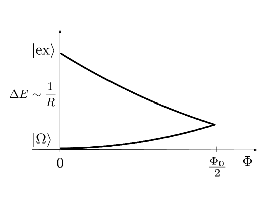
Figure 4: Kramers degeneracy at half flux.

In its original implementation for band insulators, this argument reproduces the $\mathbb{Z}_{2}$ stability index, because for $N_{f}$ fermion species, the created excitation possesses spin $N_{f}/2$, such that the Kramers degeneracy is assured for odd $N_{f}$ only. Moreover, it extends the validity of the $\mathbb{Z}_{2}$ index to systems with interactions and disorder that are time reversal invariant [11].

In an earlier work on $(2+1)$-dimensional topological insulators [13], we reformulated the stability argument in terms of properties of the partition function of edge excitations. Since the addition of half flux at the center of the Corbino disk changes the spatial boundary condition from the (A) to (P), we described the map between the corresponding partition functions, pertaining to the Neveu-Schwarz and Ramond sectors, respectively. We then analyzed the low-energy states in these partition functions and found the expected degeneracies and quantum numbers of the excitations mentioned before.

The advantage of this formulation of the stability argument is that it can be extended to any interacting system for which the partition function is known. For $(1+1)$ dimensional edges, this function can be computed for many models of the quantum spin Hall effect by using conformal field theory methods [19]. Furthermore, the general structure of the conformal partition function is known [34]: this results allowed to extend the $\mathbb{Z}_{2}$ stability index to topological insulators with Abelian and non-Abelian braidings [13]. In $(3+1)$ dimensions, we shall first formulate the argument for the fermionic surface states in this section and then extend it to bosonic systems in section 4.

2.3.1 Neveu-Schwarz sector

The natural boundary conditions for the fermion field are antiperiodic both in space and time, i.e $(\alpha_{0},\alpha_{1},\alpha_{2})=(1/2,1/2,1/2)$ in the partition function (2.29). We call this choice the Neveu-Schwarz sector, in analogy with $(1+1)$ dimensions.

The low-lying excitations in this sector can be more easily understood for a rectangular torus, setting ${\boldsymbol{\omega}}_{1}$ and ${\boldsymbol{\omega}}_{2}$ along the Cartesian axes (see Fig. 3), i.e. $\omega_{12}=\omega_{21}=0$ in (2.18). In this case the energy of excitations (2.31) has the form:

$$\mathcal{E}^{\frac{1}{2}\frac{1}{2}}_{n_{1}n_{2}}=\omega_{00}\sqrt{\left(n_{1}+\frac{1}{2}\right)^{2}\frac{1}{\omega^{2}_{11}}+\left(n_{2}+\frac{1}{2}\right)^{2}\frac{1}{\omega_{22}^{2}}}\ .$$ (2.34)

There are four low-lying degenerate energy levels, for $(n_{1},n_{2})=(0,0),(0,-1),$ $(-1,0),$ $(-1,-1)$. The expansion of the partition function gives:

$$Z^{F}_{\frac{1}{2},\frac{1}{2}\frac{1}{2}}\sim 1+\!\!\!\!\!\sum_{(n_{1},n_{2})=(0,0),(0,-1),(-1,0),(-1,-1)}\!\!\!\!\!\!\!\!\!\!\!\!\!\!\!\!\!e^{-2\pi\mathcal{E}_{\vec{n}}+2\pi i\mathcal{P}_{\vec{n}}-\omega_{00}A_{0}}+e^{-2\pi\mathcal{E}_{\vec{n}}-2\pi i\mathcal{P}_{\vec{n}}+\omega_{00}A_{0}}.$$ (2.35)

Therefore, the low-lying states are the ground state plus four particle and four antiparticle excitations; their fermion parity can be read from the definition (2.26). In particular, for the ground state,

$$(-1)^{F}\ket{\Omega}_{NS}=\ket{\Omega}_{NS},\qquad\quad(-1)^{2S}=(-1)^{F}.$$ (2.36)

In order to discuss the Fu-Kane-Mele stability argument, we need to distinguish between surface excitations with integer and half-integer spin, and to this effect, we shall introduce the ‘spin parity’ index $(-1)^{2S}$, that is equal to the fermion parity of the $(2+1)$-dimensional theory, $(-1)^{2S}=(-1)^{F}$ [13, 9].

2.3.2 Ramond sector

The first step of the stability argument consists on adiabatically inserting two $\Phi_{0}/2$ fluxes in the three-dimensional Corbino geometry (see Fig. 2). We call $V^{1/2}_{i}$, with $i=1,2$, the related transformations. These insertions modify the quantization of the momenta $k_{x}$ and $k_{y}$, i.e. the spatial boundary conditions $\alpha_{i}\rightarrow\alpha_{i}+1/2$. Starting from the Neveu-Schwarz sector $Z^{F}_{\frac{1}{2},\frac{1}{2}\frac{1}{2}}$ and applying $V^{1/2}_{1}$ and $V^{1/2}_{2}$ we obtain:

$$V^{1/2}_{1}:\Phi_{1}\to\Phi_{1}+\Phi_{0}/2,\ \ \ \ \ \ \ \ \ Z^{F}_{\frac{1}{2},\frac{1}{2}\frac{1}{2}}\longrightarrow Z^{F}_{\frac{1}{2},0\frac{1}{2}},$$ (2.37)

$$V^{1/2}_{2}:\Phi_{2}\to\Phi_{2}+\Phi_{0}/2,\ \ \ \ \ \ \ \ \ Z^{F}_{\frac{1}{2},0\frac{1}{2}}\longrightarrow Z^{F}_{\frac{1}{2},00},$$ (2.38)

eventually reaching the periodic-periodic sector with partition function $Z^{F}_{\frac{1}{2},00}$, that will be called the $(2+1)$-dimensional Ramond sector. Fig. 5 shows the transformations of all partition functions under half-flux insertions.

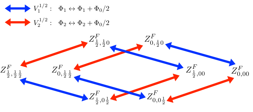
Figure 5: Transformations of partition functions $Z^{F}_{\alpha_{0},\alpha_{1}\alpha_{2}}$ under addition of half fluxes, $V^{1/2}_{1}$ and $V^{1/2}_{2}$; the indices $\alpha_{\mu}=0$ (resp. $1/2$) indicate periodic (resp. antiperiodic) boundary conditions, $\mu=0,1,2$.

In the Ramond sector, the energy and momentum (2.31)-(2.32) are vanishing for $(n_{1},n_{2})=(0,0)$, i.e $\mathcal{E}^{0,0}_{0,0}=\mathcal{P}^{0,0}_{0,0}=0$. Upon expanding the Ramond partition function, we find four degenerated states,

$$Z^{F}_{\frac{1}{2},00}\propto 1+e^{-\omega_{00}A_{0}}+e^{\omega_{00}A_{0}}+e^{-\omega_{00}A_{0}}e^{\omega_{00}A_{0}}+\dots,$$ (2.39)

that we call $\ket{v^{(i)}}$, $i=1,\dots,4$. Let us analyze their quantum numbers. Two of them have charge $Q=\pm 1$,

$$e^{-\omega_{00}A_{0}}\leftrightarrow\ket{v^{(2)}},\ \ \ \ \ \ \ e^{\omega_{00}A_{0}}\leftrightarrow\ket{v^{(3)}}.$$ (2.40)

The other two states are neutral: upon following the evolution of spectrum while adding the fluxes, i.e. $\alpha_{i}:1/2\to 0$, we can see that the Neveu-Schwarz ground state is mapped into the following Ramond state: $\ket{\Omega}_{NS}\to\ket{v^{(1)}}$. The fourth term is identified as the expected partner of the Kramers pair, $\ket{v^{(4)}}={\cal T}\ket{v^{(1)}}$,

$$1\leftrightarrow\ket{v^{(1)}},\qquad e^{-\omega_{00}A_{0}}e^{\omega_{00}A_{0}}\leftrightarrow\ket{v^{(4)}},\qquad Q\ket{v^{(1)}}=Q\ket{v^{(4)}}=0.$$ (2.41)

This identification should be checked by evaluating the spin parity of the four states, that should read:

$$(-1)^{2S}=(-1)^{F}=-1\qquad{\rm on}\qquad\ket{v^{(1)}},\ \ket{v^{(4)}},$$

$$(-1)^{2S}=(-1)^{F}=1\qquad\ \ {\rm on}\qquad\ket{v^{(2)}},\ \ket{v^{(3)}}.$$ (2.42)

We recall that the fermion number of Ramond states is well understood in $(1+1)$-dimensions, being the sum of the chiral and anti-chiral numbers, $F=F_{R}+F_{L}$ [9]. We now discuss it in $(2+1)$ dimensions, and show that it is actually independent of the dimension and the chiral splitting. The Fock space identification of these four states in the Ramond sector follows from the definitions (2.22) and the previous arguments:

$$\ket{v^{(1)}}=\ket{\Omega}_{R},\quad\ket{v^{(2)}}=a^{\dagger}_{00}\ket{\Omega}_{R},\quad\ket{v^{(3)}}=b^{\dagger}_{00}\ket{\Omega}_{R},\quad\ket{v^{(4)}}=b^{\dagger}_{00}a^{\dagger}_{00}\ket{\Omega}_{R},$$ (2.43)

where $\ket{\Omega}_{R}$ is the Ramond ground state. Let us reconsider the normal ordering of the charge and fermion number given in (2.25)-(2.26), starting from the expansion around the Fermi level of a non-relativistic spectrum at finite volume. In the case of the Neveu-Schwarz sector, the Fermi level is located in between the empty and filled states, because the energy spectrum (2.34) is strictly positive. This gives a clear identification of particles and antiparticles and determines the standard normal-ordering of the relativistic expressions used in (2.25)-(2.26).

In the Ramond sector, there is an ambiguity because some excitations are exactly located at the Fermi level. We shall assume that they are partially filled:

$$\langle a^{\dagger}_{00}a_{00}\rangle=x,\qquad\langle b^{\dagger}_{00}b_{00}\rangle=1-x,\qquad\quad 0\leq x<1.$$ (2.44)

Thus, the normal-ordered expressions of charge and fermion number (2.25)-(2.26) should be modified in the term $(n_{1},n_{2})=(0,0)$ of the sums, as follows:

$$Q=\sum_{\vec{n}}a^{\dagger}_{\vec{n}}a_{\vec{n}}-b_{\vec{n}}^{\dagger}b_{\vec{n}}+1-2x,$$ (2.45)

$$(-1)^{F}=(-1)^{\sum_{\vec{n}}a^{\dagger}_{\vec{n}}a_{\vec{n}}+b_{\vec{n}}^{\dagger}b_{\vec{n}}+1}.$$ (2.46)

Upon further assuming the particle-hole symmetric filling $x=1/2$, we obtain the quantum number assignments given before in (2.40), (2.42).

In conclusion, the Ramond states $\ket{\Omega}_{R}$ and $b^{\dagger}_{00}a^{\dagger}_{00}\ket{\Omega}_{R}$, have vanishing charge and negative spin-parity and are identified with the Kramers doublet that we were looking for. Since the Ramond sector corresponds to a time-reversal invariant point for the Hamiltonian, this degeneracy is robust to any invariant perturbation. To conclude the Fu-Kane-Mele stability argument we return to zero flux: while the Ramond ground state $\ket{\Omega}_{R}$ goes back to the Neveu-Schwarz state $\ket{\Omega}_{NS}$, its Kramers partner flows into the following excited state,

$$\ket{ex}_{NS}\ \leftrightarrow\ e^{-2\pi\mathcal{E}_{-1-1}^{\frac{1}{2}\frac{1}{2}}+\omega_{00}A_{0}}e^{-2\pi\mathcal{E}_{-1-1}^{\frac{1}{2}\frac{1}{2}}-\omega_{00}A_{0}}.$$ (2.47)

The energy of this excitation is $\mathcal{O}(1/R)$, where $R$ is the typical dimension of the system; this proves that the spectrum stays gapless (in the thermodynamic limit) for any time-reversal invariant interaction.

We remark that the neutral $S=1/2$ excitation created by adding half fluxes is a nonperturbative excitation in the fermionic theory with respect to the Neveu-Schwarz ground state,

$$\ket{\Omega}_{R}=\sigma(0)\ket{\Omega}_{NS}.$$ (2.48)

In the $(1+1)$-dimensional theory, $\sigma(x)$ is known as the ‘spin field’ and its properties are well understood, e.g. within the fermionic description of the Ising model [9]; much less is known in $(2+1)$ dimensions, to our knowledge.

The stability of the surface excitations can be related to a $\mathbb{Z}_{2}$ anomaly, as in the case of the lower dimensional topological system [13, 35]. Indeed, the Neveu-Schwarz and Ramond ground states are eigenstates of a time-reversal invariant Hamiltonian, but possess different spin-parity index, i.e.

$$(-1)^{2S}\ket{\Omega}_{NS}=\ket{\Omega}_{NS},\qquad\quad(-1)^{2S}\ket{\Omega}_{R}=-\ket{\Omega}_{R}.$$ (2.49)

The index is conserved by time reversal symmetry, but changes between two invariant ground states, without any breaking of the symmetry either explicit or spontaneous. Therefore, we interprete this change as a discrete $\mathbb{Z}_{2}$ anomaly, which is equivalent to the $\mathbb{Z}_{2}$ index of stability.

2.4 Modular transformations

In this section we study the behavior of the eight partition functions under the discrete changes of coordinates that map the three-torus into itself. The pattern of transformations will further characterize the different sectors. Moreover, we shall associate the stability of topological insulators to the impossibility of writing a modular invariant partition function that is consistent with all physical requirements. These results are close analogs of the $(2+1)$-dimensional ones [13].

In the following we set $A_{0}=0$ for simplicity, and rewrite the partition function (2.29) as follows:

$$Z^{F}_{\alpha_{0},\alpha_{1}\alpha_{2}}=e^{-VF_{0}}\prod_{n_{1},n_{2}\in\mathbb{Z}}\bigg{|}1-\exp\left(-2\pi\mathcal{E}_{n_{1},n_{2}}^{\alpha_{1}\alpha_{2}}+2\pi i\mathcal{P}_{n_{1},n_{2}}^{\alpha_{1}\alpha_{2}}-2\pi i\alpha_{0}\right)\bigg{|}^{2}.$$ (2.50)

The modular transformations of the torus $\mathbb{T}^{3}$ express the reparameterization of the moduli $({\boldsymbol{\omega}}_{0},{\boldsymbol{\omega}}_{1},{\boldsymbol{\omega}}_{2})$, and form the group $SL(3,\mathbb{Z})$. Two subgroups $SL(2,\mathbb{Z})$ act on the two-dimensional subspaces $(x_{0},x_{i})$, $i=1,2$, and have generators $T_{i}:{\boldsymbol{\omega}}_{0}\to{\boldsymbol{\omega}}_{0}+{\boldsymbol{\omega}}_{i}$ and $S_{i}:{\boldsymbol{\omega}}_{0}\to-{\boldsymbol{\omega}}_{i}$, ${\boldsymbol{\omega}}_{i}\to{\boldsymbol{\omega}}_{0}$ [9]. The three-dimensional group is generated by $T_{1}$ and $U_{1}=S_{1}P_{12}$, where $P_{12}$ is the permutation of spatial vectors, i.e. $P_{12}:{\boldsymbol{\omega}}_{1}\to-{\boldsymbol{\omega}}_{2}$, ${\boldsymbol{\omega}}_{2}\to{\boldsymbol{\omega}}_{1}$. The generators $(T_{2},S_{2})$ are clearly expressed in terms of $T_{1}$ and $S_{1}$ by $T_{2}=P_{12}T_{1}P_{12}$ and $S_{2}=P_{12}S_{1}P_{12}$.

The action of $P_{12}$ on the partition functions (2.50) is manifest: $Z^{F}_{\alpha_{0},\frac{1}{2}\frac{1}{2}}$ and $Z^{F}_{\alpha_{0},00}$ are left invariant, while the others exchange in pairs, e.g. $Z^{F}_{\alpha_{0},\frac{1}{2}0}\leftrightarrow Z^{F}_{\alpha_{0},0\frac{1}{2}}$. Therefore it is sufficient to study the modular transformations given by $T_{1}$ and $S_{1}$ and then apply $P_{12}$ to find the action of the entire group.

The action of $T_{1}$ is also simply derived from (2.50). If $\alpha_{1}=0$, the partition functions $Z^{F}_{\alpha_{0};0\alpha_{2}}$ are invariant. If $\alpha_{1}=1/2$, $T_{1}$ changes the temporal boundary conditions from $(A)$ to $(P)$ and viceversa, i.e $Z^{F}_{1/2,1/2\,\alpha_{2}}\leftrightarrow Z^{F}_{0,1/2\,\alpha_{2}}$.

The action of the transformation $S_{1}$ requires some calculations. Following [20], it is useful to choose coordinates in which the $\boldsymbol{\omega}$ matrix is triangular:

$$\boldsymbol{\omega}=\begin{pmatrix}\omega_{00}&\omega_{01}&\omega_{02}\\ 0&\omega_{11}&\omega_{12}\\ 0&0&\omega_{22}\end{pmatrix}=\begin{pmatrix}2\pi R_{0}&-2\pi\alpha R_{1}&-2\pi\gamma R_{2}\\ 0&2\pi R_{1}&-2\pi\beta R_{2}\\ 0&0&2\pi R_{2}\end{pmatrix}.$$ (2.51)

In this basis, the fermionic partition functions (2.27) and (2.28), before making the regularization of the vacuum energy, takes the following form:

$$\begin{split}Z^{F}_{\alpha_{0},\alpha_{1}\alpha_{2}}=&\prod_{n_{2}\in\mathbb{Z}}\left\{\prod_{n_{1}\in\mathbb{Z}}\left|1-\exp{\cal A}_{\vec{n}}\right|^{2}\exp{\cal B}_{\vec{n}}\right\}\ ,\\ {\cal A}_{\vec{n}}=&-2\pi r_{01}\sqrt{[(n_{1}+\alpha_{1})+\beta(n_{2}+\alpha_{2})]^{2}+[r_{12}(n_{2}+\alpha_{2})]^{2}}\\ &+2\pi i\left[\alpha(n_{1}+\alpha_{1})+(n_{2}+\alpha_{2})(\alpha\beta+\gamma)\right]-2\pi i\alpha_{0}\ ,\\ {\cal B}_{\vec{n}}=&2\pi r_{01}\sqrt{\left[(n_{1}+\alpha_{1})+\beta(n_{2}+\alpha_{2})\right]^{2}+\left[r_{12}(n_{2}+\alpha_{2})\right]^{2}}\ ,\end{split}$$ (2.52)

where we split the products on $n_{1}$ and $n_{2}$ and introduced the two quantities $r_{01}=R_{0}/R_{1}$ e $r_{12}=R_{1}/R_{2}$.

The strategy of the calculation [20] is to reduce the partition function to a product of ‘massive $\Theta$ functions’ whose $S$ transformation is know. These functions are defined by [36]:

$$\Theta_{[a,b]}(\tau;m) = \prod_{n\in\mathbb{Z}}\left|1-\exp\left[-2\pi\text{Im}(\tau)\sqrt{(n+a)^{2}+m^{2}}+2\pi i\text{Re}(\tau)(n+a)+2\pi ib\right]\right|^{2}$$ (2.53)

$$\qquad\times\exp\left[4\pi\text{Im}(\tau)\Delta(m;a)\right]\ ,$$

where $a,b,m\in\mathbb{H}^{+}$, $\tau\in\mathbb{C}$, and $\Delta(m;a)$ is given by,

$$\Delta(m;a)=-\frac{1}{2\pi^{2}}\sum_{l>0}\int_{0}^{+\infty}dt~{}e^{-\frac{\pi^{2}m^{2}}{t}-tl^{2}}\cos(2\pi la).$$ (2.54)

Identifying:

$$a=\alpha_{1}+\beta(n_{2}+\alpha_{2}),\quad b=\gamma(n_{2}+\alpha_{2})+\alpha_{0},\quad m=r_{12}(n_{2}+\alpha_{2}),$$

$$\tau=-\frac{\omega_{01}}{\omega_{11}}+i\frac{\omega_{00}}{\omega_{11}}=\alpha+ir_{01},$$ (2.55)

the fermionic partition function (2.52) can be rewritten,

$$Z^{F}_{\alpha_{0},\alpha_{1},\alpha_{2}}=\prod_{n_{2}\in\mathbb{Z}}\Theta_{[\alpha_{1}+\beta(n_{2}+\alpha_{2}),\gamma(n_{2}+\alpha_{2})+\alpha_{0}]}\left(\alpha+ir_{01};r_{12}(n_{2}+\alpha_{2})\right).$$ (2.56)

The action of $S_{1}$ in the basis (2.51) is:

$$\tau\to\ -\frac{1}{\tau},\ \ \ \ \ \ \ \ \alpha\to\ -\frac{\alpha}{\alpha^{2}+r^{2}_{02}},\ \ \ \ r_{01}\ \to\ \frac{r_{01}}{\alpha^{2}+r^{2}_{01}},$$

$$R_{0}\ \to\ \frac{R_{0}}{|\tau|},\ \ \ \ \ R_{1}\ \to\ R_{1}|\tau|,\ \ \ \ \ \ \ \ R_{2}\to R_{2},\ \ \ \ \ \gamma\ \to\ -\beta,\ \ \ \ \ \beta\ \to\ \gamma.$$ (2.57)

We now use the transformation of the massive $\Theta$ function [36],

$$\Theta_{[a,b]}(\tau;m)=\Theta_{[b,-a]}\left(-\frac{1}{\tau};m|\tau|\right).$$ (2.58)

for each factor in the partition function (2.56), to obtain:

$$\begin{split}S_{1}\ :\ &\Theta_{[\alpha_{1}+\beta(n_{2}+\alpha_{2}),\gamma(n_{2}+\alpha_{2})+\alpha_{0}]}(\tau;r_{12}(n_{2}+\alpha_{2}))\longrightarrow\\ &\qquad\Theta_{[\alpha_{1}+\gamma(n_{2}+\alpha_{2}),-\beta(n_{2}+\alpha_{2})+\alpha_{0}]}\left(-\frac{1}{\tau};r_{12}(n_{2}+\alpha_{2})|\tau|\right)=\\ &\qquad\Theta_{[-\alpha_{0}+\beta(n_{2}+\alpha_{2}),\gamma(n_{2}+\alpha_{2})+\alpha_{1}]}(\tau;r_{12}(n_{2}+\alpha_{2})),\end{split}$$ (2.59)

Finally, the $S_{1}$ transformation of the partition function sis found to be:

$$S_{1}\ :\ Z^{F}_{\alpha_{0},\alpha_{1}\alpha_{2}}(\boldsymbol{\omega}_{0},\boldsymbol{\omega}_{1},\boldsymbol{\omega}_{2})\ \to\ Z^{F}_{\alpha_{0},\alpha_{1}\alpha_{2}}(-\boldsymbol{\omega}_{1},\boldsymbol{\omega}_{0},\boldsymbol{\omega}_{2})=Z^{F}_{\alpha_{1},\alpha_{0}\alpha_{2}}(\boldsymbol{\omega}_{0},\boldsymbol{\omega}_{1},\boldsymbol{\omega}_{2}).$$ (2.60)

This behavior agrees with the expectations. All together, the pattern of modular transformations of the eight partition functions $Z^{F}_{\alpha_{0},\alpha_{1}\alpha_{2}}$ is shown in Fig. 6.

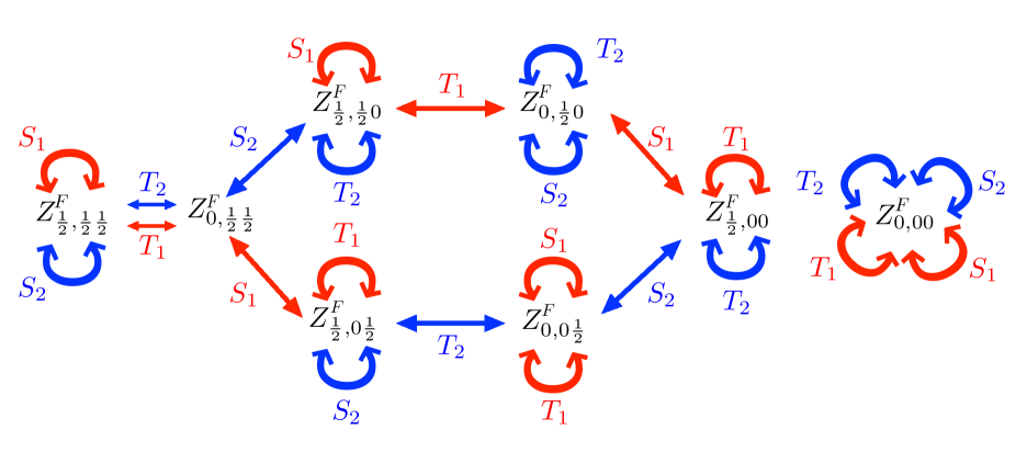
Figure 6: Pattern of modular transformations $T_{1}$, $T_{2}$, $S_{1}$, $S_{2}$ for the partition functions $Z^{F}_{\alpha_{0},\alpha_{1}\alpha_{2}}$.

2.4.1 Stability and modular invariance

The sum over the eight spin sectors,

$$Z^{F}_{\text{Ising}}=\sum_{\alpha_{0},\alpha_{1},\alpha_{2}=0,\frac{1}{2}}Z^{F}_{\alpha_{0},\alpha_{1}\alpha_{2}},$$ (2.61)

is found to be invariant under flux insertions $V^{1/2}_{1}$, $V^{1/2}_{2}$ and modular transformations by using the results in Fig. 5 and Fig. 6. We can call this modular invariant the ‘Ising partition function’ being the generalization of a typical partition function of a statistical model in two dimensions [13, 9]. However, we have seen that some sectors, such as the Neveu-Schwarz and Ramond sectors, possess different values of the ground state spin parity $(-1)^{2S}$ and cannot be part of the same theory without breaking explicitly the time reversal symmetry. Namely, the $\mathbb{Z}_{2}$ spin parity anomaly requires that the partition functions stay separate and form a eight-dimensional vector. The first component $Z^{F}_{\frac{1}{2}\frac{1}{2}\frac{1}{2}}$ describes the unperturbed time-reversal invariant surface system, while the other functions contain excited states due to changes of electromagnetic and gravitational backgrounds.

In conclusion, the stability of topological insulators has been related to the $\mathbb{Z}_{2}$ spin parity anomaly, which also implies the modular covariance of the partition function, namely a discrete gravitational anomaly [13, 9]. We mention that other authors have been relating the modular covariance of the boundary partition function to the stability of the topological phase in the bulk [37].

2.5 Dimensional reduction

In this section we further characterize the eight fermionic partition functions by performing a reduction from two to one spatial dimensions that let us recover well-known expressions [9].

Let us consider the partition functions for a rectangular torus, i.e. $\omega_{12}=\omega_{21}=0$, and vanishing scalar potential $A_{0}=0$, for simplicity. We perform a dimensional reduction of the Kaluza-Klein type, namely take the limit $R_{2}\to 0$ of the Corbino donut, such that the modes of energy $O(n_{2}/R_{2})$ are never excited, corresponding to $n_{2}\to 0$. The remaining geometry is that of two-torus in the plane $(x^{0},x^{1})$; about the energy spectrum (2.31), there are two possibilities: i) for periodic boundary condition along $x_{2}$, i.e. $\alpha_{2}=0$, the spectrum becomes exactly that of the massless fermion in $(1+1)$ dimensions; ii) for antiperiodic conditions, $\alpha_{2}=1/2$, there remains the constant $1/(4\pi R_{2})^{2}$ that plays the role of a mass in $(1+1)$-dimensions.

We start from the expression (2.27)-(2.28) before regularization of the ground state energy, and rewrite it in the coordinates (2.18):

$$Z^{F}_{\alpha_{0},\alpha_{1}\alpha_{2}} = \prod_{n_{2}}\left\{\exp\left[\frac{2\pi\omega_{00}}{\omega_{11}}\sum_{n_{1}}\sqrt{(n_{1}+\alpha_{1})^{2}+(n_{2}+\alpha_{2})^{2}\frac{\omega_{11}^{2}}{\omega_{22}^{2}}}\right]\right.$$ (2.62)

$$\quad\times\prod_{n_{1}}\bigg{|}1-\exp\bigg{(}-\frac{2\pi\omega_{00}}{\omega_{11}}\sqrt{(n_{1}+\alpha_{1})^{2}+(n_{2}+\alpha_{2})^{2}\frac{\omega_{11}^{2}}{\omega_{22}^{2}}}$$

$$\quad\quad+\frac{2\pi i\omega_{01}}{\omega_{11}}(n_{1}+\alpha_{1})+\frac{2\pi i\omega_{02}}{\omega_{22}}(n_{2}+\alpha_{2})+2\pi i\alpha_{0}\bigg{)}\bigg{|}^{2}\bigg{\}}.$$

The regularized form of the $n_{1}$ sum in the first exponent is written again in terms of the $\Delta$ function (2.54):

$$\sum_{n_{1}}\sqrt{(n_{1}+\alpha_{1})^{2}+(n_{2}+\alpha_{2})^{2}\frac{\omega_{11}^{2}}{\omega_{22}^{2}}}=\Delta\left[\frac{\omega_{11}}{\omega_{22}}(n_{2}+\alpha_{2});\alpha_{1}\right]\ .$$ (2.63)

The two-torus is specified by the modular parameter $\tau$ in (2.4). A further convenient simplification is setting $\omega_{02}=0$, i.e. no bending of this torus in three dimensions. Altogether, the expression (2.62) can be written again as a product over $n_{2}\in\mathbb{Z}$ of massive $\Theta$ functions. In the limit $\omega_{22}\to 0$, the leading behaviour is given by the factor with $n_{2}=0$; the dimensional reduction is therefore:

$$Z^{F}_{\alpha_{0},\alpha_{1}\alpha_{2}}\longrightarrow Z^{F}_{\alpha_{0},\alpha_{1}|\alpha_{2}}=\Theta_{[\alpha_{1},\alpha_{0}]}\left(\tau;\ \frac{\omega_{11}}{\omega_{22}}\alpha_{2}\right).$$ (2.64)

The reduced partition function is denoted by a vertical line before the index $\alpha_{2}$ of the direction $x_{2}\to 0$. We now analyze this expression more explicitly.

2.5.1 Massless case $\alpha_{2}=0$

In this case, the prefactor $\Delta(m;a)$ appearing in the theta-function reads:

$$\Delta(0;\alpha_{1}=0)=-\frac{1}{12},\ \ \ \ \ \ \Delta(0;\alpha_{1}=\frac{1}{2})=\frac{1}{24},$$ (2.65)

and the ground state energy prefactor becomes,

$$\text{exp}\left(4\pi\text{Im}\tau\Delta(0;\alpha_{1})\right)=\begin{cases}\left(q\bar{q}\right)^{1/12},\ \ \ \ \ \ \ \alpha_{1}=0,\\ \left(q\bar{q}\right)^{-1/24},\ \ \ \ \ \alpha_{1}=\frac{1}{2},\end{cases}$$ (2.66)

where $q=\exp{(2\pi i\tau)}$. Remembering that $\eta(q)=q^{1/24}\prod_{n=1}^{\infty}(1-q^{n})$ is the Dedekind function, the reduced partition functions (2.64) become the following expressions:

$$Z^{F}_{\frac{1}{2},\frac{1}{2}\big{|}0}=\left|\frac{1}{\eta(\tau)}\prod_{n=1}^{\infty}(1-q^{n})(1+q^{n-1/2})^{2}\right|^{2}=\left|\frac{1}{\eta(\tau)}\sum_{m\in\mathbb{Z}}q^{m^{2}/2}\right|^{2}=Z^{NS},$$ (2.67)

$$Z^{F}_{0,\frac{1}{2}\big{|}0}=\left|\frac{1}{\eta(\tau)}\prod_{n=1}^{\infty}(1-q^{n})(1-q^{n-1/2})^{2}\right|^{2}=\left|\frac{1}{\eta(\tau)}\sum_{m\in\mathbb{Z}}(-1)^{m}q^{m^{2}/2}\right|^{2}=Z^{\widetilde{NS}},$$ (2.68)

$$Z^{F}_{\frac{1}{2},0\big{|}0}=\left|\frac{1}{\eta(\tau)}2q^{1/8}\prod_{n=1}^{\infty}(1-q^{n})(1+q^{n})^{2}\right|^{2}=\left|\frac{1}{\eta(\tau)}\sum_{m\in\mathbb{Z}}q^{\left(m+1/2\right)^{2}/2}\right|^{2}=Z^{R},$$ (2.69)

$$Z^{F}_{0,0\big{|}0}=\left|\frac{1}{\eta(\tau)}q^{1/8}\prod_{n=1}^{\infty}(1-q^{n})(1-q^{n})(1-q^{n-1})\right|^{2}=Z^{\widetilde{R}}=0.$$ (2.70)

These are the well-known partition functions of the $(1+1)$-dimensional Dirac fermion that describes the edge of the two-dimensional topological insulator [13]. In these formulas, we identify the sectors $(AA),(PA),(AP),(PP)$ as $NS,\widetilde{NS},R,\widetilde{R}$, respectively. We also wrote the bosonic version of these expressions [9] for later use in Section 4. The $SL(2,\mathbb{Z})$ modular transformations of these partition functions is denoted as the ‘massless subgroup’ shown in Fig.7.

2.5.2 Massive case $\alpha_{2}=1/2$

As anticipated, in this case the (large) mass term $M=\omega_{11}/2\omega_{22}$ remains in the energy spectrum in $(1+1)$ dimensions. Therefore the reduction leads to the following four partition functions of the massive fermion, that read:

$$Z^{F}_{\frac{1}{2},\frac{1}{2}\big{|}\frac{1}{2}}=\Theta_{[\frac{1}{2},\frac{1}{2}]}(\tau;M),\ \ \ \ \ \ \ \ Z^{F}_{0,\frac{1}{2}\big{|}\frac{1}{2}}=\Theta_{[\frac{1}{2},0]}(\tau;M),$$

$$Z^{F}_{\frac{1}{2},0\big{|}\frac{1}{2}}=\Theta_{[0,\frac{1}{2}]}(\tau;M),\ \ \ \ \ \ \ \ \ Z^{F}_{0,0\big{|}\frac{1}{2}}=\Theta_{[0,0]}(\tau;M).$$ (2.71)

Their transformations under the subgroup $SL(2,\mathbb{Z})$ are the same of those of the massless sector, and are indicated as the ‘massive subgroup’ in Fig.7.

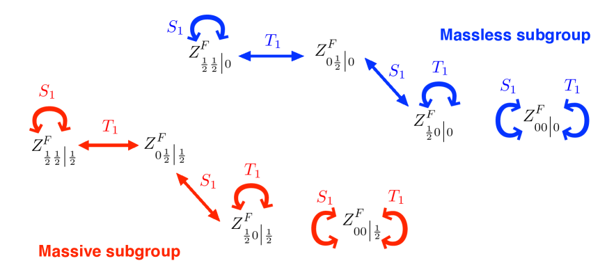
Figure 7: Action of the modular group $SL(2,\mathbb{Z})$ over of the eight fermionic partition functions (2.67)-(2.71) dimensionally reduced to the $(x^{0},x^{1})$ plane.

3 Bosonic topological insulators

In this section, we discuss the effective field theory description of free and interacting topological insulators in $(3+1)$ dimensions given by the topological BF gauge theory and the associated bosonic surface theory. We shall recall some known facts, derive the action at the boundary, its quantization and the partition function on the three-torus. We shall then compare these results with those found in the previous section for the fermionic theory and discuss the insight they provide on bosonization in $(2+1)$ dimensions.

The motivations for introducing bosonic degrees of freedom in $(3+1)$ dimensional topological states are the following:

• The great success of bosonic theories in explaining interacting topological states in $(2+1)$ dimensions, starting from the original work by Wen on the fractional quantum Hall effect, that provided a complementary view to wavefunction approaches [7]. Furthermore, the conformal field theories describing edge states and braiding relations are usually formulated in terms of bosonic fields [9].

• In particular, the canonical quantization of the compactified free boson theory in $(1+1)$ dimensions (the so-called chiral Luttinger liquid) provides an exact description of interacting Hall edge states with Abelian fractional statistics [30]; this approach can be generalized to topological insulators by taking pairs of theories with opposite chirality and spin [10, 13].

• Such an approach actually corresponds to the BF bulk theory [16], that can be naturally extended to $(3+1)$ dimensions [15], where it accounts for particle-vortex braiding relations and other topological effects [38].

• We can thus study the corresponding bosonic surface theory in $(2+1)$ dimensions and the dynamics it can support [8]. Of course, an exact map between fermions and bosons cannot be achieved [39]; nonetheless, we shall find some physical properties that do not depend on interactions and can be described exactly.

• Finally, there are topological states in $(3+1)$ dimensions that are formulated in terms of bosonic microscopic degrees of freedom [40].

3.1 Hydrodynamic BF effective action

We consider low-energy matter fluctuations that are described by the conserved currents $J^{\mu}$ for quasiparticles and $J^{\mu\nu}$ for vortices: these can be expressed in terms of two hydrodynamic gauge fields,

$$J^{\mu}=\frac{1}{2\pi}\varepsilon^{\mu\nu\rho\sigma}\partial_{\nu}b_{\rho\sigma},\qquad J^{\mu\nu}=\frac{1}{2\pi}\varepsilon^{\mu\nu\rho\sigma}\partial_{\rho}a_{\sigma},$$ (3.1)

that are the two-form $b=1/2\,b_{\mu\nu}\,dx^{\mu}\wedge dx^{\nu}$ and the one-form $a=a_{\mu}dx^{\mu}$. The topological effects in time-reversal invariant topological states at energies below the bulk gap can be described by the following BF action, with first order derivatives and gauge symmetries $a\to a+d\lambda$ and $b\to b+d\xi$ [16, 8],

$$S_{BF}[a,b,A]=\int_{\mathcal{M}}\frac{K}{2\pi}b\,da+\frac{1}{2\pi}b\,dA-\frac{\theta}{8\pi^{2}}\,da\,dA+a_{\mu}{\cal J}^{\mu}+\frac{1}{2}b_{\mu\nu}{\cal J}^{\mu\nu}\ ,$$ (3.2)

where $A=A_{\mu}dx^{\mu}$ is the electromagnetic background and ${\cal J}_{\mu}$, ${\cal J}_{\mu\nu}$ are sources for quasiparticle and vortex excitations. The time reversal transformations of the fields are: $a_{\mu}=(a_{0},\vec{a})\to(a_{0},-\vec{a})$, $A_{\mu}=(A_{0},\vec{A})\to(A_{0},-\vec{A})$ and $b_{\mu\nu}=(b_{0i},b_{ij})\to(-b_{0i},b_{ij})$, for $\mu=(0,i)$. Thus, the theory is invariant but for the term proportional to $\theta$. The coupling $K$ is an odd integer for fermionic systems [38].

Same features of the BF theory are:

• For $A_{\mu}=0$, the solutions of the equations of motion in presence of the sources, i.e.

  $${\cal J}^{\mu\nu}=\frac{K}{2\pi}\epsilon^{\mu\nu\lambda\rho}\partial_{\lambda}a_{\rho}\ ,\qquad{\cal J}^{\mu}=\frac{K}{4\pi}\epsilon^{\mu\lambda\rho\nu}\partial_{\lambda}b_{\rho\nu}\ ,$$ (3.3)

  imply a non-trivial monodromy of quasiparticles around vortices in three space dimensions, with Aharonov-Bohm phases $\varphi=2\pi N_{0}N_{1}/K$, where $N_{0},N_{1}$ are the quasiparticle electric charge and the vortex magnetic charge, respectively.

• For ${\cal J}^{\mu}=0,{\cal J}^{\mu\nu}=0$, one can compute the induced action for the electromagnetic background by integrating the hydrodynamic fields [8],

  $$S_{\text{ind}}[A]=\frac{\theta}{8\pi^{2}K}\int_{\cal M}dA\,dA=\frac{\theta}{32\pi^{2}K}\int d^{4}x~{}\epsilon^{\mu\nu\lambda\rho}F_{\mu\nu}F_{\lambda\rho}\ .$$ (3.4)

  This the Abelian theta therm already discussed in the previous section (2.16)[16]: the case $\theta=0$ corresponds to the time reversal invariant system, where bulk and boundary contributions cancel each other (See Section 2.1). For $\theta=\pi$, time reversal symmetry is broken at the surface, leading to the induced Chern-Simons term,

  $$S_{\text{ind}}[A]=\frac{1}{8\pi K}\int_{\partial\cal M}A\,dA\ ,$$ (3.5)

  implying a surface quantum Hall effect with filling fraction $\nu=1/2K$. In particular, for $K=1$ the fermion anomaly (2.15) is recovered.

• This is the first indication that the bosonic theory for $K=1$ matches the fermionic description, at least for the topological properties. Other values of $K$ describe interacting theories with quasiparticle-vortex braiding statistics.

• For manifolds $\cal M$ with a boundary, an additional surface action should be introduced to compensate for the gauge non-invariance of the BF theory (3.2) [8]. This is:

  $$S_{\rm surf}[\zeta,a,A]=-\int_{\partial\mathcal{M}}\frac{K}{2\pi}\zeta da+\frac{1}{2\pi}\zeta dA,$$ (3.6)

where the one-form gauge field $\zeta=\zeta_{\mu}dx^{\mu}$ absorbs the gauge transformation of the $b$ field, namely $b\to b+d\xi$ and $\zeta\to\zeta+\xi$.

3.2 Surface bosonic theory

In this section we discuss the massless excitations at the surface and introduce two dynamics for them that are compatible with the bulk BF theory and time reversal invariance. Note in passing that the $(2+1)$-dimensional boundary may also support massive phases with topological excitations, whose induced action precisely cancels the Chern-Simons term from the bulk [41]. These cases will not be discussed here.

The action (3.6) (putting $A_{\mu}=0$ momentarily) involves boundary degrees of freedom can be viewed as (singular) gauge configurations reproducing the bulk loop observables, namely $b=d\zeta$ and $a=d\phi$, where $\zeta$ and $\phi$ are a vector and a scalar field, respectively. The topological BF theory implies a vanishing Hamiltonian, i.e. the static case; after choosing the gauge $\zeta_{0}=a_{0}=0$, the action (3.6) becomes,

$$S_{\rm surf}=\frac{K}{2\pi}\int d^{3}x\,\epsilon^{ij}\partial_{i}\zeta_{j}\,\dot{\phi}.$$ (3.7)

This expression shows that there are two scalar degrees of freedom at the surface, $\phi$ and $\chi$, that are canonically conjugate, being the longitudinal part of $a_{i}=\partial_{i}\phi$, and the transverse part of $\zeta_{i}=\epsilon_{ik}\partial_{k}\chi$, respectively,

$$S_{\rm surf}=\int d^{3}x\,\pi\,\dot{\phi},\qquad\pi=\frac{K}{2\pi}\epsilon^{ij}\partial_{i}\zeta_{j}=-\frac{K}{2\pi}\Delta\chi.$$ (3.8)

Since the surface excitations possess a relativistic dynamics, we should add a Hamiltonian. We first consider the free scalar Hamiltonian in $(2+1)$ dimensions, as follows [8]:

$$S_{\rm surf}\to\int d^{3}x\left(\pi\dot{\phi}-{\cal H}(\pi,\phi)\right)=\int d^{3}x\left(\pi\dot{\phi}-\frac{1}{2m}\pi^{2}-\frac{m}{2}(\partial_{i}\phi)^{2}\right)\ .$$ (3.9)

In this equation, we introduced a mass parameter for adjusting the mismatch of dimensions between bulk and boundary: indeed, the bulk gauge fields imply the mass dimensions $[\phi]=0$ and $[\pi]=2$, which are different from those of the three-dimensional scalar theory $1/2$ and $3/2$, respectively. A dimensionless coupling could also be introduced for the third therm in the action (3.9), that would determine the Fermi velocity of excitations. This is conventionally fixed to one. The equations of motion of the action (3.9) are:

$$\pi=m\dot{\phi},\qquad\dot{\pi}=m\Delta\phi\ ,$$ (3.10)

and the Lagrangian form of the action is clearly

$$S_{\rm surf}=\frac{m}{2}\int d^{3}x\ \left(\partial_{\mu}\phi\right)^{2}.$$ (3.11)

The Hamiltonian equations of motion (3.10) can be recast into a duality relation between the boundary scalar and vector fields, that can be written in covariant form (with $\zeta_{0}=0$)[17]:

$$\frac{K}{2\pi}\,\epsilon^{\mu\nu\rho}\partial_{\nu}\zeta_{\rho}=m\,\partial_{\mu}\phi.$$ (3.12)

This is the just the electric-magnetic duality in $(2+1)$ dimensions: it plays a role in the bosonization of $(2+1)$-dimensional fermions through the tomographic representation [39, 8] and other approaches [18]. In our setting, this duality is just the first-order Hamiltonian description of the relativistic wave equation, that is inherited from the first-order bulk theory. We also stress that the main motivation for introducing the Hamiltonian (3.9) is its simplicity. On one side, we know that the surface fermion of the previous section cannot be exactly matched to a free boson (for $K=1$). On another side, any dynamics of bosonic states that can model interacting fermions is interesting to investigate at the present stage of understanding of $(3+1)$-dimensional topological insulators.

The coupling to the electromagnetic field $A_{\mu}$ can be used to test the correspondence between boson and fermion theories. The coupling inherited from the bulk theory is shown in (3.6) and it amounts to the shift $a_{\mu}\to a_{\mu}+A_{\mu}/K$. This can be implemented in the symplectic form (3.7) (using the gauge condition $\partial_{i}A_{i}=0$) and in the Hamiltonian (3.9), thus leading to the following action:

$$S_{\rm surf}[\zeta,\phi,A]=\int d^{3}x\left[\pi\left(\dot{\phi}-\frac{A_{0}}{K}\right)-\frac{1}{2m}\pi^{2}-\frac{m}{2}\left(\partial_{i}\phi-\frac{A_{i}}{K}\right)^{2}\right].$$ (3.13)

Upon integrating the scalar fields, we obtain the induced action,

$$S_{\rm ind}^{B}[A]=\frac{m}{2K^{2}}\int d^{3}x\ F_{\mu\nu}\frac{1}{\Box}F_{\mu\nu}\ .$$ (3.14)

This result should be compared for $K=1$ with the fermionic induced action computed in Section 2.1: using Eq. (2.14), we disregard the anomalous term cancelled by the bulk and obtain the expression for $m\to 0$:

$$S^{F}_{\rm ind}[A]\sim\int d^{3}x\,F_{\mu\nu}\frac{1}{\Box^{1/2}}\left(1+O\left(\frac{m^{2}}{\Box}\right)\right)F_{\mu\nu}\ .$$ (3.15)

We thus find that the bosonic and fermionic induced actions, (3.14) and (3.15) do not match, to leading quadratic order in $A_{\mu}$; one difference is given by the explicit dimensionful parameter of the bosonic theory. This could be scaled out by the field redefinition,

$$\widetilde{\phi}=\sqrt{m}\phi,\qquad\widetilde{\zeta_{i}}=\frac{\zeta_{i}}{\sqrt{m}},\qquad\widetilde{\pi}=\frac{1}{\sqrt{m}}\pi,$$ (3.16)

but it would not change the induced action (3.14), unless a corresponding shift is considered for the electromagnetic coupling. This is not justified because it would imply different bulk and boundary responses for topological insulators.

We now introduce another Hamiltonian for the bosonic surface states that is also compatible with the symplectic structure (3.7) and relativistic invariance. Let us reconsider the duality relation between vector and scalar fields (3.12) and modify it as follows:

$$\frac{K}{2\pi}\,\epsilon^{\mu\nu\rho}\partial_{\nu}\zeta_{\rho}=\Box^{1/2}\,\partial_{\mu}\phi,$$ (3.17)

by replacing the mass parameters with a Lorentz invariant non-local operator. This modified duality corresponds to the following Hamiltonian equations of motion:

$$\pi=\frac{K}{2\pi}\varepsilon^{ij}\partial_{i}\zeta_{j}=\Box^{1/2}\dot{\phi},\qquad\dot{\pi}=\Box^{1/2}\Delta\phi,$$ (3.18)

that follow from the action,

$$S^{\prime}_{\rm surf}=\int d^{3}x\left(\pi\dot{\phi}-\frac{1}{2}\pi\frac{1}{\Box^{1/2}}\pi-\frac{1}{2}\partial_{i}\phi\,\Box^{1/2}\partial_{i}\phi\right)\ .$$ (3.19)

In Lagrangian formulation, this reads:

$$S^{\prime}_{\rm surf}=-\frac{1}{2}\int\phi\,\Box^{3/2}\phi=\frac{1}{2}\int\left(\partial_{\mu}\widetilde{\phi}\right)^{2},\qquad\phi=\Box^{1/4}\widetilde{\phi},$$ (3.20)

that is again the free bosonic theory in the rescaled field variable $\widetilde{\phi}$. The coupling to the electromagnetic field implied by the bulk theory is still given by the Higgs-like substitution, $\partial_{\mu}\phi\to\partial_{\mu}\phi+A_{\mu}/K$, leading to the action:

$$S^{\prime}_{\rm surf}[\phi,A]=\frac{1}{2}\int d^{3}x\left(\partial_{\mu}\phi-\frac{A_{\mu}}{K}\right)\Box^{1/2}\left(\partial_{\mu}\phi-\frac{A_{\mu}}{K}\right).$$ (3.21)

Upon integration of the scalar field, we obtain the induced action $S^{B^{\prime}}_{\rm ind}$ that is equal to the fermionic expression $S^{F}_{\rm ind}$ (3.15) up to a constant. Therefore, the non-local bosonic theory (3.19) has the same response to weak electromagnetic backgrounds as the fermionic theory.

We note that a Lagrangian similar to (3.15) was also introduced in the studies of bosonization of Refs.[39] Although legitimate for a massless theory, a non-local effective action usually means that further massless excitations have been integrated out. This may indicate that the dynamics (3.19) is incomplete.

In conclusion, we have shown that the surface degrees of freedom of $(3+1)$ dimensional topological insulators amount to a Hamiltonian conjugate pair of scalar fields. The simpler quadratic Hamiltonian for them is not able to reproduce the fermionic electromagnetic response to leading order, while a modified non-local dynamics does work. The two theories are identical on-shell, since both imply the free wave equation for suitably rescaled field variables, but may differ in the solitonic excitations.

These open issues are left for further investigations; we remark again that the analysis in the rest of this paper will deal with properties that are independent of the specific dynamics. It is nevertheless important to stress that the topological data in $(3+1)$ dimensions given by the BF action (3.2) do not determine a unique dynamics for the surface states, contrary to the case of $(2+1)$-dimensional topological insulators.

We finally remark that the local action (3.20) with coupling to electromagnetic field given by (3.21) is equivalent to the Abelian Higgs model in $(2+1)$ dimensions in the deep infrared limit of the spontaneously broken phase. Namely, the scalar field $\phi$ is the Goldstone mode of a complex scalar:

$$\Phi=\rho\,{\rm e}^{i\phi}\ ,\qquad\quad\langle\rho^{2}\rangle=m\ ,$$ (3.22)

while the mass parameter $m$ fixes the vacuum expectation value, i.e. the Higgs field is frozen. We conclude that in cases where the electromagnetic field could be considered dynamic, we could have a superconducting phase at the surface of the topological insulator. On the other hand, the nonlocal dynamics (3.21) would keep the photon massless as in the fermionic theory.

3.3 Canonical quantization of the compactified boson in $(2+1)$ dimensions

In this section we consider the canonical quantization of the compactified boson with action (3.8), (3.9) and compute its partition functions on the three-torus. We shall pay particular attention to the properties of solitonic modes of the $\phi$ and $\zeta_{i}$ fields, in such a way that they consistently reproduce the topological properties of the bulk BF theory. We shall follow the analysis of Ref.[21] and extend it in some directions that are rather relevant for the final result. Some background knowledge can be found in the quantization of the compactified chiral boson in $(1+1)$ dimensions of Ref[30]. The quantization of the other non-local theory (3.21) is left for future investigations.

3.3.1 Bulk topological sectors and boundary observables

The quantization of the BF theory (3.7) on the spatial three-torus ${\cal M}=\mathbb{T}^{3}\times\mathbb{R}$, leads to the topological order of $K^{3}$ ‘anyon’ sectors, for odd integer values of the coupling $K$. The proof of this results is very simple [1]: one considers the integrals of the gauge fields $b$ and $a$ on the surfaces and cycles of the torus, respectively:

$$\pi_{ij}=\int_{\Sigma_{ij}}b,\quad i\neq j,\qquad\quad q_{i}=\int_{\gamma_{i}}a,\qquad\quad i,j,k=1,2,3.$$ (3.23)

These integrals define the global variables $(\pi_{ij}(t),q_{k}(t))$; once inserted into the BF action, they become three pairs of canonically conjugate variables. The canonical quantization yields the following commutation relations:

$$\left[\pi_{ij}(t),q_{k}(t)\right]=i\frac{2\pi}{K}\varepsilon_{ijk}\ .$$ (3.24)

A basis of holonomies on the torus is given by the operators $U_{i}=\exp(iq_{i})$ and $V_{ij}=\exp(i\pi_{ij})$: they form three pairs of $K$-dimensional clock and shift matrices, thus leading to a $K^{3}$-dimensional representation, namely to the topological order $K^{3}$. In the following, we find a corresponding symplectic structure among the solitonic modes of the boundary fields $\phi,\zeta_{i}$, that are defined on the space-time three-torus.

The relation between bulk and boundary observables can be studied on the spatial geometry of the thick two-torus $V=D^{2}\times S^{1}$, whose boundary is the two-torus $\partial V=S^{1}\times S^{1}$. We first consider a bulk quasiparticle with charge $N_{0}$ at rest in $\vec{x}=\vec{x}_{0}$, whose current is ${\cal J}^{0}(\vec{x})=N_{0}\delta^{(3)}(\vec{x}-\vec{x}_{0})$ (see Fig. 8(a)). The solution of the equations of motion (3.3) leads to a flux of the $b$ field across a surface enclosing the charge [21], that becomes the following expression on the boundary surface:

$$\frac{2\pi N_{0}}{K}=\int_{\partial V}d^{2}x\,\epsilon^{ij}\partial_{i}\zeta_{j}.$$ (3.25)

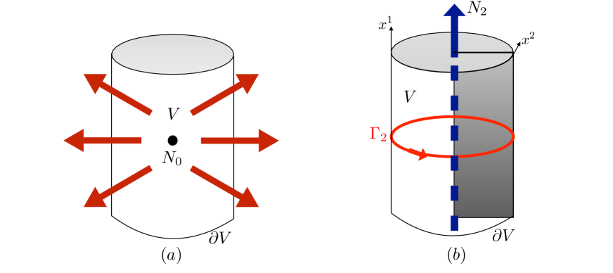
Figure 8: (a) Flux due to the electric charge $N_{0}$ in the bulk; (b) Bulk vortex of magnetic charge $N_{2}$ along $x^{1}$ and closed line $\Gamma_{2}$ encircling it on the surface. In grey the branch cut surface from the vortex excitation to the boundary.

A static vortex in the bulk stretched along the non-trivial cycle with magnetic charge $N_{2}$ corresponds to the current ${\cal J}^{01}(\vec{x})=N_{2}\delta^{(2)}(\vec{x}-\vec{x}_{0})$ (see Fig. 8(b)). The equations of motion imply a non-vanishing integral of the $a$ field along a closed path encircling the vortex; for the path $\Gamma_{2}$ on the boundary surface, it reads:

$$\frac{2\pi}{K}N_{2}=\oint_{\Gamma_{2}}dx^{2}\partial_{2}\phi\ .$$ (3.26)

An analogous relation holds for the other non-trivial cycle of the boundary,

$$\frac{2\pi}{K}N_{1}=\oint_{\Gamma_{1}}dx^{1}\partial_{1}\phi\ .$$ (3.27)

3.3.2 Quantization

The bosonic action (3.9) is considered on the space-time geometry $\partial{\cal M}=\partial V\times\mathbb{R}=S^{1}\times S^{1}\times\mathbb{R}$. The conjugate momentum $\pi$ is:

$$\pi=\frac{K}{2\pi}\epsilon^{ij}\partial_{i}\zeta_{j}\ ,$$ (3.28)

and the Hamiltonian equations of motion are,

$$\frac{K}{2\pi}\epsilon^{ij}\partial_{i}\zeta_{j}=m\dot{\phi}\ ,\qquad\frac{K}{2\pi}\epsilon^{ij}\partial_{i}\dot{\zeta_{j}}=m\Delta\phi\ .$$ (3.29)

The canonical quantization proceeds by expanding the fields in terms of solutions of the equations of motion, with boundary conditions of the spatial two-torus specified by the periods $\vec{\omega}_{i}$ (2.19) and dual vectors $\vec{k}_{i}$ (2.21), $i=1,2$. Let us write the field expansions and then explain them:

$$\phi(\vec{x},t)=\phi_{0}+2\pi\Lambda_{i}\vec{k}_{i}\cdot\vec{x}+\frac{K\Lambda_{0}t}{mV^{(2)}}$$

$$\qquad+\frac{1}{\sqrt{mV^{(2)}}}\sum_{\vec{n}\neq(0,0)}\frac{1}{\sqrt{2E_{\vec{n}}}}\left[a_{\vec{n}}\ \text{e}^{-iE_{\vec{n}}t+2\pi i\vec{k}_{\vec{n}}\cdot\vec{x}}+a^{\dagger}_{\vec{n}}\ \text{e}^{iE_{\vec{n}}t-2\pi i\vec{k}_{\vec{n}}\cdot\vec{x}}\right],$$ (3.30)

$$\zeta_{j}(\vec{x},t)=\frac{\epsilon_{ji}}{V^{(2)}}\left(\omega_{2i}\gamma_{1}-\omega_{1j}\gamma_{2}-\pi\Lambda_{0}x_{i}\right)$$

$$\qquad+\frac{8\pi^{2}}{K}\sqrt{\frac{m}{V^{(2)}}}\sum_{\vec{n}\neq(0,0)}\frac{\epsilon_{jm}\left(n_{1}k_{1m}+n_{2}k_{2m}\right)}{\left(2E_{\vec{n}}\right)^{3/2}}\left[a_{\vec{n}}\ \text{e}^{-iE_{\vec{n}}t+2\pi i\vec{k}_{\vec{n}}\cdot\vec{x}}+a^{\dagger}_{\vec{n}}\ \text{e}^{iE_{\vec{n}}t-2\pi i\vec{k}_{\vec{n}}\cdot\vec{x}}\right].$$ (3.31)

These expressions involve oscillating functions specified by energies and momenta

$$E_{\vec{n}}=2\pi\left|n_{1}\vec{k}_{1}+n_{2}\vec{k}_{2}\right|=\frac{2\pi}{V^{(2)}}\left|n_{1}\vec{\omega}_{2}-n_{2}\vec{\omega}_{1}\right|,$$ (3.32)

$$\vec{k}_{\vec{n}}=\left(k_{1\vec{n}},k_{2\vec{n}}\right)=\frac{1}{V^{(2)}}\left(n_{1}\omega_{22}-n_{2}\omega_{12},\ -n_{1}\omega_{21}+n_{2}\omega_{11}\right)\ .$$ (3.33)

The field expansions (3.3.2),(3.3.2) also contain constant and linear terms, almost unconstrained by the equations of motion, that are needed for specifying the solitonic modes. Actually, upon inserting these expressions in the boundary observables (3.25)-(3.27), we find the following values of the $\zeta_{i}$ flux and $\partial_{i}\phi$ circulations:

$$\Lambda_{\mu}=\frac{N_{\mu}}{K},\qquad\quad\alpha=0,1,2\ ,$$ (3.34)

that explain the normalizations adopted in (3.3.2), (3.3.2).

The commutation relations between the fields $\phi$ and $\pi$,

$$\left[\phi(\vec{x},t),\varepsilon^{ij}\partial_{i}\zeta_{j}(\vec{y},t)\right]=i\frac{2\pi}{K}\delta^{(2)}(\vec{x}-\vec{y}),$$ (3.35)

imply the following non-vanishing commutators:

$$\left[a_{\vec{n}},a^{\dagger}_{\vec{k}}\right]=\delta_{\vec{n},\vec{k}},\qquad\quad\left[\phi_{0},\Lambda_{0}\right]=\frac{i}{K}.$$ (3.36)

Moreover, integrating by parts the symplectic term in the action (3.7), we can also consider $\zeta_{i}$ and $\varepsilon^{ij}\partial_{j}\phi$, for $i=1,2$, as two pairs of coordinates and momenta, leading to two further commutation relations:

$$\left[\zeta_{i}(\vec{x},t),\epsilon_{ij}\partial_{j}\phi(\vec{y},t),\right]=-i\frac{2\pi}{k}\delta^{(2)}(\vec{x}-\vec{y}),\qquad i=1,2.$$ (3.37)

These are independent relations for the solitonic modes only; they imply the earlier quantizations plus the following ones:

$$\left[\gamma_{1},\Lambda_{2}\right]=-\frac{i}{K},\qquad\quad\left[\gamma_{2},\Lambda_{1}\right]=\frac{i}{K}.$$ (3.38)

These two commutation relations together with that of $\Lambda_{0}$ in (3.36) represent the bulk degrees of freedom (3.23) within the boundary theory: one quantity in each pair parameterizes the bulk observable evaluated at the boundary, i.e. $\Lambda_{\mu}=(\Lambda_{0},\Lambda_{1},\Lambda_{2})$, while the conjugate variable is a field zero mode, $(\phi_{0},\gamma_{2},\gamma_{1})$. After quantization, the eigenvalues of $\Lambda_{\mu}$ can be identified with the spectra (3.34), that are consistent with the periodicities of the field zero modes,

$$\phi_{0}\equiv\phi_{0}+2\pi r,\qquad\gamma_{i}\equiv\gamma_{i}+2\pi r_{i},\quad i=1,2,$$ (3.39)

for compactification radii $r=r_{1}=r_{2}=1$. It is also immediate to see that these periodicities are commensurate with those of the fields $\phi(\vec{x}),\zeta_{i}(\vec{x})$ winding around the cycles of the torus. In conclusion, the $\Lambda_{\mu}$ spectra (3.34) are both suggested by the bulk theory and consistently obtained by quantization of the boundary theory. The same result holds in the better-known quantization of the bosonic theory in $(1+1)$ dimensions at the edge of the quantum Hall effect [30]. We remark that in both bosonic theories, there are other consistent values of the compactification radii, but they would imply solitonic spectra that are not related to the bulk topological data and should be discarded.

The Hamiltonian and the momenta are expressed in terms of Fock and solitonic operators by substituting the field expansions (3.3.2)-(3.3.2) into standard field expressions of the bosonic theory (3.9). The results are:

$$H=\frac{K^{2}\Lambda^{2}_{0}}{2mV^{(2)}}+\frac{(2\pi)^{2}m}{2V^{(2)}}\left[\left(\Lambda_{1}\omega_{22}-\Lambda_{2}\omega_{12}\right)^{2}+\left(\Lambda_{1}\omega_{21}-\Lambda_{2}\omega_{11}\right)^{2}\right]$$

$$\ \ \ +\sum_{\vec{n}\neq(0,0)}E_{\vec{n}}\left(a^{\dagger}_{\vec{n}}a_{\vec{n}}+\frac{1}{2}\right),$$ (3.40)

$$P^{1}=\frac{2\pi k\Lambda_{0}}{V^{(2)}}\left(-\Lambda_{1}\omega_{22}+\Lambda_{2}\omega_{12}\right)+2\pi\sum_{\vec{n}\neq(0,0)}k_{1\vec{n}}\ a^{\dagger}_{\vec{n}}a_{\vec{n}},$$ (3.41)

$$P^{2}=\frac{2\pi k\Lambda_{0}}{V^{(2)}}\left(\Lambda_{1}\omega_{21}-\Lambda_{2}\omega_{11}\right)+2\pi\sum_{\vec{n}\neq(0,0)}k_{2\vec{n}}\ a^{\dagger}_{\vec{n}}a_{\vec{n}},$$ (3.42)

where the energies $E_{\vec{n}}$ are momenta $\vec{k}_{\vec{n}}$ are given in (3.32)-(3.33).

3.4 Bosonic partition functions

We now compute the partition functions by compactifying the time direction, i.e. taking the trace over the states. The sums over the bosonic Fock space and solitonic modes can be done independently, because their contributions add up in the expressions of Hamiltonian (3.3.2) and momentum (3.41), (3.42). Thus, the partition function can be factorized into solitonic and oscillator parts $Z^{(0)}$ and $Z_{HO}$, respectively

$$Z^{B}=Z^{(0)}Z_{HO}.$$ (3.43)

The straightforward calculations of the traces on the spectra (3.3.2) -(3.42) is done by using the coordinates (2.19) and (2.21), then the resulting expressions are written in covariant $(2+1)$-dimensional notation as functions of the moduli $\boldsymbol{\omega}_{\mu}$, leading to:

$$Z_{HO}=\exp(F)\prod_{(n_{1},n_{2})\neq(0,0)}\bigg{(}1-\text{exp}\left(-2\pi\mathcal{E}_{\vec{n}}+2\pi i\mathcal{K}_{\vec{n}}\right)\bigg{)}^{-1},$$ (3.44)

and

$$Z^{(0)}=\sum_{\Lambda_{\mu}\in\mathbb{Z}^{3}/K}\exp\bigg{[} -\frac{V^{(3)}}{|\boldsymbol{\omega}_{1}\times\boldsymbol{\omega}_{2}|^{2}}\left(\frac{K^{2}\Lambda^{2}_{0}}{2m}+2\pi^{2}m|\Lambda_{1}\boldsymbol{\omega}_{2}-\Lambda_{2}\boldsymbol{\omega}_{1}|^{2}\right)$$

$$-\frac{i2\pi K\Lambda_{0}}{|\boldsymbol{\omega}_{1}\times\boldsymbol{\omega}_{2}|^{2}}\left(\boldsymbol{\omega}_{1}\times\boldsymbol{\omega}_{2}\right)\cdot\left(\Lambda_{1}\boldsymbol{\omega}_{0}\times\boldsymbol{\omega}_{2}-\Lambda_{2}\boldsymbol{\omega}_{0}\times\boldsymbol{\omega}_{1}\right)\bigg{]},$$ (3.45)

with

$$F=\frac{V^{(3)}}{4\pi}\sum_{(n_{1},n_{2})\neq(0,0)}\frac{1}{|n_{1}\boldsymbol{\omega}_{2}-n_{2}\boldsymbol{\omega}_{1}|^{3}},\qquad\mathcal{E}_{\vec{n}}=V^{(3)}\ \frac{|n_{1}\boldsymbol{\omega}_{2}-n_{2}\boldsymbol{\omega}_{1}|}{|\boldsymbol{\omega}_{1}\times\boldsymbol{\omega}_{2}|^{2}},$$ (3.46)

$$\mathcal{K}_{\vec{n}}=\frac{(\boldsymbol{\omega}_{1}\times\boldsymbol{\omega}_{2})}{|\boldsymbol{\omega}_{1}\times\boldsymbol{\omega}_{2}|^{2}}\left(n_{1}\boldsymbol{\omega}_{0}\times\boldsymbol{\omega}_{2}-n_{2}\boldsymbol{\omega}_{0}\times\boldsymbol{\omega}_{1}\right).$$ (3.47)

The vacuum energy $F$ is regularized by analytic continuation as in the fermionic case [33]. These results are in agreement with those found in Ref.[21].

3.4.1 Spin sectors of the bosonic theory

The experience with topological insulators in $(2+1)$ dimensions and bosonization of edge excitations [13] suggests that the partition function just found (3.44)-(3.4) should possess the following properties:

• $Z^{B}$ should split into the sum over $K^{3}$ terms, each one pertaining to an anyon sectors with given fractional values of the charges of the theory.

• Further partition functions should be found that correspond to different quantizations of the solitonic modes, and could be associated to the eight fermionic spin sectors of the three-torus.

• As in the fermionic case, these eight functions should transform one into another by adding half-flux quanta and changing modular parameters.

Let us gradually derive these results in the $(3+1)$-dimensional theory. The anyon sectors can be identified by splitting the summations over the charge lattice $\Lambda_{\mu}\in\mathbb{Z}^{3}/K$ in $Z^{(0)}$ (3.4) into integer and fractional values, by substituting:

$$\Lambda_{\mu}=M_{\mu}+\frac{m_{\mu}}{K},\qquad M_{\mu}\in\mathbb{Z},\qquad\ m_{\mu}=0,1,\cdots,K-1,\qquad\mu=0,1,2.$$ (3.48)

In this way we get the $K^{3}$ terms, each one involving summations over integer-spaced charges only, as follows:

$$Z^{(0)}=\sum_{\Lambda_{\mu}\in\mathbb{Z}^{3}/K}\cdots=\sum_{m_{0},m_{1},m_{2}=0}^{K-1}\ \sum_{M_{0},M_{1},M_{2}\in\mathbb{Z}}\cdots=\sum_{m_{0},m_{1},m_{2}=0}^{K-1}Z^{(0)\,m_{0}m_{1}m_{2}}.$$ (3.49)

In Section 2.3, we formulated the flux insertion argument for the stability of topological insulators in terms of fermionic partition functions. Starting from the Neveu-Schwarz sector, we added half fluxes through the donut and obtained the other spin sectors of the theory. In the bosonic theory, adding fluxes clearly modify the values of the loop observables (3.26),(3.27): for example, one flux $\Phi_{0}$ adds one unit of magnetic charge to the corresponding vortex, causing $N_{i}\to N_{i}+1$, $i=1,2$. This is in agreement with the coupling to $A_{\mu}$ in (3.13).

For $K=1$ adding one flux is clearly a symmetry of the Hamiltonian (3.3.2) and of the partition function (3.49), owing to the summation over $\Lambda_{i}\equiv N_{i}\in\mathbb{Z}$; thus, we should consider adding half fluxes by the transformations,

$$V^{1/2}_{i}:\ \ \ \ \Phi_{i}\ \to\ \Phi_{i}+\frac{\Phi_{0}}{2}\qquad\quad\Lambda_{i}\ \to\ \Lambda_{i}+\frac{1}{2},\qquad i=1,2.$$ (3.50)

that shifts the $\Lambda_{i}$ summation variables. For $K>1$ odd, again building on the experience in $(2+1)$ dimension [13, 10], we should add a number of fluxes that do not change the anyon sector, i.e. the fractional value of $\Lambda_{i}$. Thus, we consider the transformations:

$$V^{K/2}_{i}:\ \ \ \ \Lambda_{i}=M_{i}+\frac{m_{i}}{2}\ \to\ \Lambda_{i}+\frac{1}{2},\qquad i=1,2.$$ (3.51)

We shall introduce three labels $\alpha_{\mu}=0,1/2$, $\mu=0,1,2$ to the partition function (3.43), as follows:

$$Z^{B}_{\alpha_{0},\alpha_{1}\alpha_{2}}=Z_{HO}\,Z^{(0)}_{\alpha_{0},\alpha_{1}\alpha_{2}},\qquad\quad\alpha_{0},\alpha_{1},\alpha_{2}=0,\frac{1}{2}.$$ (3.52)

Two of them, $\alpha_{1},\alpha_{2}$, specify the half-integer values taken by the variables $M_{1},M_{2}$ after flux insertions (3.51), while $\alpha_{0}=1/2$ amounts to adding the sign $(-1)^{K\Lambda_{0}}$ to the summand in (3.4) for reasons that will be clear in the following. Note that oscillator part $Z_{HO}$ stays invariant. In conclusion, we have the following eight partition functions:

$$Z^{B}_{\alpha_{0},\alpha_{1}\alpha_{2}}= \sum_{m_{\mu}\in\mathbb{Z}^{3}_{K}}Z_{\alpha_{0},\alpha_{1}\alpha_{2}}^{B\,m_{0}m_{1}m_{2}}$$

$$= Z_{HO}\sum_{m_{\mu}\in\mathbb{Z}^{3}_{K}}\sum_{M_{\mu}\in\mathbb{Z}^{3}}(-1)^{2\alpha_{0}K\Lambda_{0}}$$

$$\qquad\times\exp\bigg{[}-\frac{V^{(3)}}{|\boldsymbol{\omega}_{1}\times\boldsymbol{\omega}_{2}|^{2}}\left(\frac{K^{2}\Lambda^{2}_{0}}{2m}+2\pi^{2}m|\Lambda_{1}\boldsymbol{\omega}_{2}-\Lambda_{2}\boldsymbol{\omega}_{1}|^{2}\right)$$

$$\qquad-\frac{i2\pi K\Lambda_{0}}{|\boldsymbol{\omega}_{1}\times\boldsymbol{\omega}_{2}|^{2}}\left(\boldsymbol{\omega}_{1}\times\boldsymbol{\omega}_{2}\right)\cdot\left(\Lambda_{1}\boldsymbol{\omega}_{0}\times\boldsymbol{\omega}_{2}-\Lambda_{2}\boldsymbol{\omega}_{0}\times\boldsymbol{\omega}_{1}\right)\bigg{]},$$ (3.53)

with parameters,

$$\Lambda_{0}=M_{0}+\frac{m_{0}}{K},\qquad \Lambda_{1}=M_{1}+\frac{m_{1}}{K}+\alpha_{1},\qquad\Lambda_{2}=M_{2}+\frac{m_{2}}{K}+\alpha_{2},$$

$$\alpha_{0},\alpha_{1},\alpha_{2}=0,\frac{1}{2}.$$ (3.54)

These partition functions are mapped one into another by the flux insertions $V^{K/2}_{i}$, $i=1,2$ as shown in Fig. 9. A characterization of these functions as the bosonic analogues of the fermionic spin sectors will become clear in the following discussion.

4 Bosonization in $(2+1)$ dimensions

In this section we focus on the set of eight bosonic partition functions $Z^{B}_{\alpha_{0},\alpha_{1}\alpha_{2}}$ for $K=1$. We show that they have the same modular transformations and other properties of the fermionic functions $Z^{F}_{\alpha_{0},\alpha_{1}\alpha_{2}}$. We then argue that these quantities are actually describing a fermionic theory, although different from the free theory of Section 2. Our results provide an exact instance of bosonization in $(2+1)$ dimensions, namely on the correspondence between (interacting) fermion and boson theories. It concerns the transformation properties of the spectrum under changes of backgrounds, that are actually independent of the dynamics and thus can be studied in the free limit of the two theories.

The fermionic characterization of the bosonic partition functions will be based on the following properties:

• The bosonic $Z^{B}_{\alpha_{0},\alpha_{1}\alpha_{2}}$ and fermionic $Z^{F}_{\alpha_{0},\alpha_{1}\alpha_{2}}$ transform in the same way under modular transformations and flux insertions.

• Within each sector, they become equal under dimensional reduction to $(1+1)$ dimensions, where the free bosonic and fermionic theories match exactly.

• The fermion number parity is associated to the states of the bosonic theory, and checked under dimensional reduction.

• The stability argument for fermionic topological states of Section 2 is reformulated in the bosonic theory for $K=1$ and extended to $K>1$, thus proving the stability of fractional topological insulators with odd integer $K$.

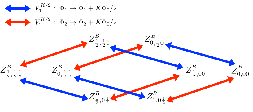
Figure 9: $V^{K/2}_{1}$ and $V^{K/2}_{2}$ flux transformations on the bosonic partition functions $Z^{B}_{\alpha_{0},\alpha_{1}\alpha_{2}}$.

4.1 Modular transformations

We recall from Section 2.4 that the action of the modular group $SL(3,\mathbb{Z})$ is described by the generators $T_{1}$, $S_{1}$ and $P_{12}$. Their action on the oscillator $Z_{HO}$ and solitonic $Z^{(0)}_{\alpha_{0},\alpha_{1},\alpha_{2}}$ factors of the partition functions will be described in turn.

Under the $P_{12}$ transformation,

$$P_{12}:\ \ \ \ \ \ {\boldsymbol{\omega}}_{0}\ \to\ {\boldsymbol{\omega}}_{0},\ \ \ \ \ {\boldsymbol{\omega}}_{1}\ \to\ -{\boldsymbol{\omega}}_{2},\ \ \ \ \ {\boldsymbol{\omega}}_{2}\ \to\ {\boldsymbol{\omega}}_{1},$$ (4.1)

we find that $Z_{HO}$ (3.44) is manifestly invariant. The action on the solitonic part $Z^{(0)}$ (3.4.1) (for $K=1$) is equivalent to the relabeling of the variables $(N_{1}\to-N_{2},\ N_{2}\to N_{1})$, whose values are integer or half integer depending on the values of $\alpha_{1},\alpha_{2}$. Thus, we find

$$P_{12}:\ \ \ \ Z^{B}_{\alpha_{0},\alpha_{1}\alpha_{2}}\ \to\ Z^{B}_{\alpha_{0},\alpha_{2}\alpha_{1}}\ ,\qquad\alpha_{1},\alpha_{2}=0,\frac{1}{2}\ .$$ (4.2)

The transformation,

$$T_{1}:\ \ \ {\boldsymbol{\omega}}_{0}\ \to\ {\boldsymbol{\omega}}_{0}+{\boldsymbol{\omega}}_{1},$$ (4.3)

leaves again $Z_{HO}$ invariant. The solitonic partitions do not change under $T_{1}$ if $M_{1}$ takes integer values; for half-integer values, the sums acquire the factor $(-1)^{M_{0}}$, thus changing the value of the index $\alpha_{0}$ from zero to $1/2$ in $Z^{B}_{\alpha_{0},\alpha_{1}\alpha_{2}}$ (3.4.1).

The action of the transformation $S_{1}$ is obtained by following the same strategy of the fermionic case in Section 2.4 [20]. We first choose the coordinates given in (2.51); the solitonic part of the partition function $Z^{(0)}_{0,00}$ in (3.4.1) takes the form ($K=1$):

$$Z^{(0)}_{0,00}=\sum_{M_{\mu}\in\mathbb{Z}^{3}}\text{exp} \bigg{(}-\frac{\tau_{2}M^{2}_{0}}{4\pi mR_{2}}\ -\ \frac{\tau_{2}m(2\pi)^{3}}{2R_{2}}\left[R_{2}^{2}\left(M_{1}+\beta M_{2}\right)^{2}+R_{1}^{2}M_{2}^{2}\right]$$

$$+2\pi i\alpha M_{0}\left(M_{1}+\beta M_{2}\right)+2\pi i\gamma M_{0}M_{2}\bigg{)},$$ (4.4)

with parameters defined as,

$$\tau=\tau_{1}+i\tau_{2}=-\frac{\omega_{01}}{\omega_{11}}+i\frac{\omega_{00}}{\omega_{11}}=\alpha+ir_{01},\ \ \ \ \ \ \frac{\omega_{12}}{\omega_{22}}=-\beta,\ \ \ \ \ \ \ \frac{\omega_{02}}{\omega_{22}}=-\gamma,$$ (4.5)

and $r_{01}=R_{0}/R_{1}$. The expressions of the functions for other $\alpha_{\mu}$ values are found by replacing $M_{1}\to M_{1}+1/2$, $M_{2}\to M_{2}+1/2$ and inserting the factor $(-1)^{M_{0}}$. The transformation of this expression is,

$$S_{1}:\ \ \ \ \ \ \ Z^{(0)}_{0,00}\left(\tau,R_{0},R_{1},R_{2},\beta,\gamma\right)\ \to\ Z^{(0)}_{0,00}\left(-\frac{1}{\tau},\frac{R_{0}}{|\tau|},R_{1}|\tau|,R_{2},\gamma,-\beta\right).$$ (4.6)

The first step is to apply the Poisson resummation formula [9] on the $M_{0}$ sum, i.e.

$$\sum_{M_{0}\in\mathbb{Z}}\text{exp}\left(-\pi AM_{0}^{2}+2\pi iM_{0}B\right)=\frac{1}{\sqrt{A}}\sum_{M_{0}^{\prime}\in\mathbb{Z}}\text{exp}\left(-\frac{\pi}{A}\left(M_{0}^{\prime}-B\right)^{2}\right).$$ (4.7)

Then, another resummation is done on the $M_{1}$ index and the result is recast into the original function $Z^{(0)}_{0,00}(\tau,R_{0},R_{1},R_{2},\beta,\gamma)$ times the factor $|\tau|$.

The oscillator part, in the chosen frame and before regularization of the vacuum energy, reads

$$Z_{HO}=\prod_{\vec{n}\neq(0,0)} \bigg{[}\left(1-\text{exp}\left(-2\pi\tau_{2}\sqrt{(n_{1}+\beta n_{2})^{2}+(n_{2}r_{12})^{2}}-2\pi i(\alpha n_{1}+n_{2}(\gamma+\tau_{1}\beta))\right)\right)^{-1}$$

$$\quad\times\text{exp}\left(-\pi\tau_{2}\sqrt{(n_{1}+\beta n_{2})^{2}+(n_{2}r_{12})^{2}}\right)\bigg{]}.$$ (4.8)

The product over $(n_{1},n_{2})$ is separated in the ranges $(n_{1}\in\mathbb{Z}\neq 0,n_{2}=0)$ and $(n_{1}\in\mathbb{Z},n_{2}\in\mathbb{Z}\neq 0)$. The first product, after regularization of the zero point energy, gives the inverse modulus square of the Dedekind functions $|\eta(\tau)|^{-2}$, where $q=\text{exp}(2\pi i\tau)$. The second factor can be rewritten in terms of the massive theta functions introduced in Section 2 (2.53), finally leading to the expression

$$Z_{HO}(\tau,R_{0},R_{1},R_{2},\beta,\gamma)=\left|\frac{1}{\eta(q)}\right|^{2}\prod_{n_{2}>0}\Theta^{-1}_{[\beta n_{2},n_{2}\gamma]}(\tau,r_{12}n_{2}).$$ (4.9)

In this form, the $S_{1}$ transformation, acting on torus parameters as in (2.4), can be evaluated for each $\Theta$ factor. The Dedekind function obeys $\eta(-1/\tau)=\sqrt{-i\tau}\,\eta(\tau)$ [9], and of theta function transforms as given in (2.58). It follows that:

$$Z_{HO}\left(-\frac{1}{\tau},\frac{R_{0}}{|\tau|},R_{1}|\tau|,R_{2},\gamma,-\beta\right) =\left|\frac{1}{\eta\left(-1/\tau\right)}\right|^{2}\prod_{n_{2}>0}\Theta_{[\gamma n_{2},-\beta n_{2}]}\left(-\frac{1}{\tau};r_{12}n_{2}|\tau|\right)$$

$$=\frac{1}{|\tau|}\left|\frac{1}{\eta(q)}\right|^{2}\prod_{n_{2}>0}\Theta_{[\beta n_{2},\gamma n_{2}]}(\tau;r_{12}n_{2})$$

$$=\frac{1}{|\tau|}Z_{HO}(\tau,R_{0},R_{1},R_{2},\beta,\gamma).$$ (4.10)

In summary,

$$S_{1}:\ \ \ \ \ Z^{B}_{0,00}\ \to\ Z^{B}_{0,00}.$$ (4.11)

Following the steps illustrated above, we find for the other partition functions the expected results ($K=1$)

$$S_{1}:\ \ \ \ Z^{B}_{\alpha_{0},\alpha_{1}\alpha_{2}}(\boldsymbol{\omega}_{0},\boldsymbol{\omega}_{1},\boldsymbol{\omega}_{2})\ \ \ \longrightarrow\ \ \ Z^{B}_{\alpha_{1},\alpha_{0}\alpha_{2}}(\boldsymbol{\omega}_{0},\boldsymbol{\omega}_{1},\boldsymbol{\omega}_{2}).$$ (4.12)

Finally, the complete set of modular transformations is shown in Fig. 10. This pattern of transformations as well as that for flux insertions in Fig. 9 are identical to those of the fermionic theory in Figs. 5 and 6, provided that the $Z^{B}_{\alpha_{0},\alpha_{1}\alpha_{2}}$ are put in suitable positions. Before establishing a correspondence term to term we still need two steps: the dimensional reduction and a change of basis that we now discuss.

Figure 10: Action of the three-dimensional modular group on the bosonic partition functions $Z^{B}_{\alpha_{0},\alpha_{1}\alpha_{2}}$.

4.2 Dimensional reduction

In this section we further characterize the eight bosonic partition functions $Z^{B}_{\alpha_{0};\,\alpha_{1}\alpha_{2}}$ by performing a dimensional reduction from two to one spatial dimensions, as done in Section 2.5 for fermions. The mapping to well-know relations of two-dimensional bosonization [9] will give useful informations on the nature of the $(2+1)$-dimensional bosonic sectors.

Let us consider the bosonic partition functions (3.4.1) with $K=1$ for a rectangular torus in the spatial directions, i.e. $\omega_{12}=\omega_{21}=0$, for simplicity. We perform again the Kaluza-Klein dimensional reduction $R_{2}\to 0$, such that the oscillating and solitonic modes of energy, respectively, $O(n_{2}/R_{2})$ and $O(M_{2}/R_{2})$, are never excited, corresponding to $n_{2},M_{2}\to 0$. Upon setting $\omega_{02}=0$, the remaining geometry is that of two-torus in the plane $(x^{0},x^{1})$, with modular parameter $\tau$ defined in (4.5). The reduction of the oscillator part $Z_{HO}$ in Eq.(4.1) clearly gives:

$$Z_{HO}(\tau)\bigg{|}_{n_{2}=0}=\left|\frac{1}{\eta(\tau)}\right|^{2}.$$ (4.13)

The solitonic factors $Z^{(0)}_{\alpha_{0};\,\alpha_{1}\alpha_{2}}$ are similarly expanded for $\omega_{22}\to 0$. Note that the classical action (3.9) would vanish in this limit, as well as the solitonic modes. Thus, we should also vary the mass that appears as a factor, $m\to\infty$, such that the following product remains finite,

$$m\omega_{22}=r^{2}/\pi,\qquad{\rm finite},\qquad\omega_{22}\to 0.$$ (4.14)

We then find the $(1+1)$-dimensional limit:

$$Z^{(0)}_{0,0|0}=\sum_{M_{0},M_{1}\in\mathbb{Z}}q^{\frac{1}{2}\left(\frac{M_{0}}{2r}+rM_{1}\right)^{2}}\overline{q}^{\frac{1}{2}\left(\frac{M_{0}}{2r}-rM_{1}\right)^{2}}.$$ (4.15)

This shows that $r$ is the compactification radius of the scalar field in $(1+1)$ dimensions, that is fixed to $r=1$ for mapping to the free fermion [9]. Similar expressions are obtained for the reductions of the other functions $Z^{(0)}_{\alpha_{0},\alpha_{1}|0}$, by shifting the integers $N_{1},N_{2}$, and adding the sign as indicated in (3.4.1),(3.4.1).

The reduction of the partition functions with $\alpha_{2}=1/2$ and $r=1$ leads to the result

$$Z^{B}_{0,0\left|\frac{1}{2}\right.}=\left(q\overline{q}\right)^{\omega^{2}_{11}/8\omega^{2}_{22}}\left|\frac{1}{\eta(\tau)}\right|^{2}\sum_{M_{0},M_{1}\in\mathbb{Z}}q^{\frac{1}{2}\left(\frac{M_{0}}{2}+M_{1}\right)^{2}}\overline{q}^{\frac{1}{2}\left(\frac{M_{0}}{2}-M_{1}\right)^{2}}\ .$$ (4.16)

This expression differs from (4.15) for the overall ground state energy $E_{0}=O(1/R^{2}_{2})\to\infty$, due to the minimal energy of waves with twisted boundary conditions, that should be subtracted for a finite limit. Note that in the fermionic dimensional reduction of Section 2.5, the same factor corresponded to a mass in the dispersion relation (2.31). After reduction, the modular transformations of bosonic functions split again into two $SL(2,\mathbb{Z})$ subgroups, as shown in Fig.11.

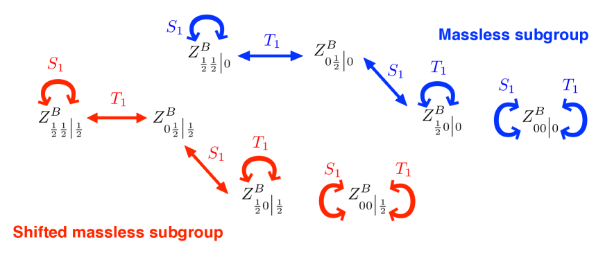
Figure 11: Action of the two-dimensional modular group over of the eight bosonic partition functions $Z^{B}_{\alpha_{0}\alpha_{1}|\alpha_{2}}$ dimensionally reduced to the $(x^{0},x^{1})$ plane.

It is convenient to rewrite the expressions (4.15), (4.16) in terms of the fermionic functions for the spin sectors $NS,\widetilde{NS},R,\widetilde{R}$, by using the bosonization formulae given in (2.67)-(2.70). The rewriting of (4.15) requires the following standard manipulations [9]: splitting in two equal parts, substituting $(M_{0},M_{1})=(2\ell,n)$ (resp. $(M_{0},M_{1})=(2\ell-1,n)$ in the first (resp. second) part, then replacing $\ell+n=\alpha_{0}$, $\ell-n=-\overline{\alpha}_{0}$ in both of them. Next, the constraint $\alpha_{0}-\overline{\alpha}_{0}=2\ell$ can be enforced by inserting the projector $\left(1+(-1)^{\alpha_{0}+\bar{\alpha}_{0}}\right)/2$ into the sums, finally obtaining:

$$Z^{B}_{0,0|0}=\frac{1}{2}\left|\frac{1}{\eta}\right|^{2} \sum_{\alpha_{0},\overline{\alpha}_{0}\ \in\mathbb{Z}}\bigg{(}q^{\frac{1}{2}\alpha_{0}^{2}}\bar{q}^{\frac{1}{2}\overline{\alpha}_{0}^{2}}+(-1)^{\alpha_{0}+\overline{\alpha}_{0}}q^{\frac{1}{2}\alpha_{0}^{2}}\bar{q}^{\frac{1}{2}\overline{\alpha}_{0}^{2}}$$

$$+q^{\frac{1}{2}\left(\alpha_{0}+\frac{1}{2}\right)^{2}}\bar{q}^{\frac{1}{2}\left(\overline{\alpha}_{0}+\frac{1}{2}\right)^{2}}+(-1)^{\alpha_{0}+\overline{\alpha}_{0}}q^{\frac{1}{2}\left(\alpha_{0}+\frac{1}{2}\right)^{2}}\bar{q}^{\frac{1}{2}\left(\overline{\alpha}_{0}+\frac{1}{2}\right)^{2}}\bigg{)}.$$ (4.17)

Namely, we find:

$$Z^{B}_{0,0|0}=\frac{1}{2}\left(Z^{NS}+Z^{\widetilde{NS}}+Z^{R}+Z^{\widetilde{R}}\right)=Z_{\text{Dirac}}.$$ (4.18)

The other one-dimensional limits of the partition functions become, following similar steps:

$$Z^{B}_{\frac{1}{2},0\big{|}0}=\frac{1}{2}\left(Z^{NS}+Z^{\widetilde{NS}}-Z^{R}-Z^{\widetilde{R}}\right)\quad\sim Z^{B}_{\frac{1}{2},0\big{|}\frac{1}{2}},$$ (4.19)

$$Z^{B}_{0,\frac{1}{2}\big{|}0}=\frac{1}{2}\left(Z^{NS}-Z^{\widetilde{NS}}+Z^{R}-Z^{\widetilde{R}}\right)\quad\sim Z^{B}_{0,\frac{1}{2}\big{|}\frac{1}{2}},$$ (4.20)

$$Z^{B}_{\frac{1}{2},\frac{1}{2}\big{|}0}=\frac{1}{2}\left(-Z^{NS}+Z^{\widetilde{NS}}+Z^{R}-Z^{\widetilde{R}}\right)\sim Z^{B}_{\frac{1}{2},\frac{1}{2}\big{|}\frac{1}{2}}.$$ (4.21)

In these formulae, we removed the zero-point energies from the partition functions with $\alpha_{2}=1/2$.

4.3 Fermion parity in the bosonic theory

Equations (4.18)-(4.21) show that under dimensional reduction the eight bosonic partition functions $Z^{B}_{\alpha_{0},\alpha_{1}\alpha_{2}}$ become linear combinations of fermionic sectors $NS,\widetilde{NS},R,\widetilde{R}$. Since $\widetilde{NS}$ and $\widetilde{R}$ involve sums of states with fermion parity $(-1)^{\cal F}$ in $(1+1)$ dimensions, we find that the linear combinations obtained by dimensional reduction realize the projectors $(1\pm(-1)^{\cal F})$ as in (4.2). Namely, they identify $(1+1)$-dimensional states of given parity, being the same for the Neveu-Schwarz and Ramond sectors. This result is summarized in the following table:

$$\begin{array}[]{l|c|c|l|l}&NS&R&{\rm positive\ Z}&{\rm indefinite\ Z}\\ \hline\cr(-1)^{\cal F}&1&1&Z^{B}_{0,0|0}\,,\ Z^{B}_{0,0|\frac{1}{2}}&Z^{B}_{\frac{1}{2},0|0}\,,\ Z^{B}_{\frac{1}{2},0|\frac{1}{2}}\\ (-1)^{\cal F}&-1&-1&Z^{B}_{0,\frac{1}{2}|0}\,,\ Z^{B}_{0,\frac{1}{2}|\frac{1}{2}}&Z^{B}_{\frac{1}{2},\frac{1}{2}|0}\,,\ Z^{B}_{\frac{1}{2},\frac{1}{2}|\frac{1}{2}}\end{array}$$ (4.22)

In this table, we also distinguish the partition functions that are sums of positive terms, corresponding to $\alpha_{0}=0$, from those with negative signs, for $\alpha_{0}=1/2$, that are due to the factor $(-1)^{M_{0}}$ in the definition (3.4.1).

We now discuss the definition of the fermion parity $(-1)^{F}$ in the bosonic theory in $(2+1)$ dimensions. Lacking a precise construction of fermionic fields in this theory, we shall adopt a practical approach. A state in $(2+1)$ dimensions will be identified as fermionic if it matches a $(1+1)$ dimensional fermionic state under dimensional reduction. We should consider both the limits $x_{2}\to 0$ given by (4.22) and $x_{1}\to 0$, corresponding to exchanging $\alpha_{1}\leftrightarrow\alpha_{2}$. Following this identification, we obtain the table:

$$\begin{array}[]{ll|c}&Z&(-1)^{F}\\ \hline\cr Z^{B}_{000}\,,&Z^{B}_{\frac{1}{2},00}&1\\ Z^{B}_{0,\frac{1}{2}\frac{1}{2}}\,,&Z^{B}_{\frac{1}{2},\frac{1}{2}\frac{1}{2}}&-1\\ Z^{B}_{0,\frac{1}{2}0}\,,&Z^{B}_{0,0\frac{1}{2}}&/\\ Z^{B}_{\frac{1}{2},\frac{1}{2}0}\,,&Z^{B}_{\frac{1}{2},0\frac{1}{2}}&/\end{array}$$ (4.23)

The first four partition functions have states with definite fermion parity, because both dimensional reductions gives the same assignment. The other four functions have no fermion parity assignment, denoted by $(/)$, because the two dimensional reductions give different results. For example, $Z^{B}_{0,\frac{1}{2}0}$ would have fermionic states according to the dimensional reduction $x_{2}\to 0$, i.e. $Z^{B}_{0,\frac{1}{2}|0}$ in table (4.22), and bosonic states under the reduction $x_{1}\to 0$, corresponding to $Z^{B}_{0,0|\frac{1}{2}}$. The nature of solitonic states in these four sectors is unclear: they could correspond to non-local degrees of freedom in the fermionic theory that are neither bosonic nor fermionic.

4.4 Bosonic Neveu-Schwarz and Ramond sectors in $(2+1)$ dimensions

In the analysis of the fermionic theory, we were able to identify $(2+1)$-dimensional analogs of the partition functions for Neveu-Schwarz and Ramond sectors, that are sums of positive terms and possess the low-energy expansions:

$$NS:\quad Z^{F}_{\frac{1}{2},\frac{1}{2}\frac{1}{2}}\sim 1+\cdots,\qquad\quad R:\quad Z^{F}_{\frac{1}{2},00}\sim 2+\cdots.$$ (4.24)

The first state in the $NS$ sector is the ground state and is bosonic, while the lowest doublet of the $R$ sector is fermionic. These sectors are mapped one into another by half-flux insertions, according to Fig. 5; moreover they occupy a definite position in the pattern of modular transformations, as shown in Fig. 6.

In the following, we want to identify bosonic functions that possess these same properties and, moreover, became equal to the corresponding fermionic functions under reduction to $(1+1)$ dimensions.

According to the patter of bosonic modular transformations shown in Fig. 10, one would be led to the identification $Z^{B}_{\alpha_{0},\alpha_{1}\alpha_{2}}\sim Z^{F}_{\alpha_{0},\alpha_{1}\alpha_{2}}$; however, the bosonic functions go into sums of fermionic sectors under dimensional reduction, and moreover, the would-be bosonic $NS$ sector $Z^{B}_{\frac{1}{2},\frac{1}{2}\frac{1}{2}}$ is not a sum of positive terms, that is not physically acceptable. Note also that dimensional reduction and fermion parity assignments would favor $Z^{B}_{000}$ as the candidate $NS$ sector, but this does not have correct modular properties.

The solution to this puzzle is found by considering a change of basis among the bosonic functions that is an isometry with respect to the action of the modular group and flux insertions. Let us first write this transformation and then discuss its features. The map between the original eight-dimensional basis,

$$Z^{B}=(Z^{B}_{\frac{1}{2},\frac{1}{2}\frac{1}{2}},\ Z^{B}_{0,\frac{1}{2}\frac{1}{2}},\ Z^{B}_{\frac{1}{2},\frac{1}{2}0},\ Z^{B}_{0,\frac{1}{2}0},\ Z^{B}_{\frac{1}{2},0\frac{1}{2}},\ Z^{B}_{0,0\frac{1}{2}},\ Z^{B}_{\frac{1}{2},00},\ Z^{B}_{0,00}),$$ (4.25)

and the new basis $Z^{\prime B}=MZ^{B}$ is given by the following matrix:

$$M=\frac{1}{2}\begin{pmatrix}-1&1&1&1&1&1&1&1\\ 1&-1&1&1&1&1&1&1\\ 1&1&-1&1&1&1&1&1\\ 1&1&1&-1&1&1&1&1\\ 1&1&1&1&-1&1&1&1\\ 1&1&1&1&1&-1&1&1\\ 1&1&1&1&1&1&-1&1\\ 1&1&1&1&1&1&1&-1\\ \end{pmatrix}.$$ (4.26)

This transformation leaves invariant the patterns of modular transformations and flux insertions given in Fig. 10 and Fig. 9, respectively; namely, $M$ commutes with $T_{i},S_{i},V^{1/2}_{i}$, for $i=1,2$. Furthermore, it is unique up to exchanges of space coordinates $x_{1}\leftrightarrow x_{2}$, that is the up-down reflection of the patterns of transformations.

The idea behind the derivation of (4.26) is very simple: the action of the modular group in Fig. 10 shows that there are two invariants given by the sum of the first seven elements of the multiplet in (4.25) and by the last element $Z^{B}_{0,00}$. In the new basis, the eighth component should be either the sum or the difference of the two invariants; the first choice is not correct because it would also invariant under flux insertions. The second choice yields the other components of the matrix $M$ by the action of flux and modular transformations.

4.4.1 Neveu-Schwarz sector

In the new basis, we are ready to identify the bosonic analogue of the Neveu-Schwarz sector, that is:

$$Z^{\prime B}_{\frac{1}{2},\frac{1}{2}\frac{1}{2}}\ \longleftrightarrow\ Z^{F}_{\frac{1}{2},\frac{1}{2}\frac{1}{2}}\ ,$$ (4.27)

as suggested by the position occupied in the patterns of transformations. The superposition of bosonic function is given by:

$$Z^{\prime B}_{\frac{1}{2},\frac{1}{2}\frac{1}{2}}=\frac{1}{2}\left(-Z^{B}_{\frac{1}{2},\frac{1}{2}\frac{1}{2}}+Z^{B}_{0,\frac{1}{2}\frac{1}{2}}+Z^{B}_{\frac{1}{2},\frac{1}{2}0}+Z^{B}_{0,\frac{1}{2}0}+Z^{B}_{\frac{1}{2},0\frac{1}{2}}+Z^{B}_{0,0\frac{1}{2}}+Z^{B}_{\frac{1}{2},00}+Z^{B}_{0,00}\right).$$ (4.28)

This expression involves sums of terms with positive integer coefficients, owing to the presence of the projectors $(-(-1)^{M_{0}}+1)/2$ in the first pair of functions and $((-1)^{M_{0}}+1)/2$ in the other pairs.

The low-energy expansion of the partition functions is done by inspecting the energy spectrum of solitonic modes (3.3.2) ($K=1$),

$$\mathcal{E}_{M_{0}M_{1}M_{2}}^{\alpha_{1}\alpha_{2}}=\frac{M_{0}^{2}}{2mV^{(2)}}+\frac{(2\pi)^{2}m}{2V^{(2)}}\left|\left(M_{1}+\alpha_{1}\right){\boldsymbol{\omega}}_{2}-\left(M_{2}+\alpha_{2}\right){\boldsymbol{\omega}}_{1}\right|^{2}.$$ (4.29)

This vanishes for $\alpha_{1}=\alpha_{2}=0$ and $M_{0}=M_{1}=M_{2}=0$ and the relative state is found in the term $(Z^{B}_{\frac{1}{2},00}+Z^{B}_{0,00})/2$ in (4.28). It gives:

$$Z^{\prime B}_{\frac{1}{2},\frac{1}{2}\frac{1}{2}}\sim 1+\cdots.$$ (4.30)

This state can be identified with the Neveu-Schwarz, i.e. unperturbed, ground state of the fermionic system: it is neutral, since $M_{0}=0$, and bosonic owing to the fermion parity assignments (4.23) to the functions $Z^{B}_{\frac{1}{2},00}$ and $Z^{B}_{0,00}$. The identification of the ground state is further confirmed by dimensional reduction. Applying the limits (4.18)-(4.21) to the linear combination in (4.28), we see that the reductions for $x_{2}\to 0$ or $x_{1}\to 0$ gives the same result by construction, and reads:

$$Z^{\prime B}_{\frac{1}{2},\frac{1}{2}\frac{1}{2}}\ \to\ \frac{1}{2}\left(Z^{NS}+Z^{\widetilde{N}S}+Z^{R}-Z^{\widetilde{R}}\right)+\left(\exp(-E_{0})\right)Z_{NS}\ ,$$ (4.31)

where $E_{0}$ is the energy shift for $\alpha=1/2$ in the circle going to zero. Therefore, the $(2+1)$-dimensional Neveu-Schwarz ground state maps into its $(1+1)$-dimensional analog, as expected. In summary, we found the following properties of the bosonic Neveu-Schwarz ground state in $(2+1)$ dimensions,

$$1\leftrightarrow\ket{\Omega}_{NS},\quad H\ket{\Omega}_{NS}=Q\ket{\Omega}_{NS}=0,\quad(-1)^{F}\ket{\Omega}_{NS}=(-1)^{2S}\ket{\Omega}_{NS}=\ket{\Omega}_{NS}.$$ (4.32)

4.4.2 Ramond sector

The $(2+1)$-dimensional Ramond sector is found by doing half-flux insertions $V_{i}^{1/2}$, $i=1,2$, that map $Z^{\prime B}_{\frac{1}{2},\frac{1}{2}\frac{1}{2}}\ \to\ Z^{\prime B}_{\frac{1}{2},00}$. The corresponding linear combination of bosonic partition functions (4.25) is given by:

$$Z^{\prime B}_{\frac{1}{2},00}=\frac{1}{2}\left(Z^{B}_{\frac{1}{2},\frac{1}{2}\frac{1}{2}}+Z^{B}_{0,\frac{1}{2}\frac{1}{2}}+Z^{B}_{\frac{1}{2},\frac{1}{2}0}+Z^{B}_{0,\frac{1}{2}0}+Z^{B}_{\frac{1}{2},0\frac{1}{2}}+Z^{B}_{0,0\frac{1}{2}}-Z^{B}_{\frac{1}{2},00}+Z^{B}_{0,00}\right).$$ (4.33)

This expression is again a sum of terms with positive integer coefficients.

Let us analyze the levels with lower energies (4.29) that are present in the four pairs $(\pm Z^{B}_{\frac{1}{2}\alpha_{1}\alpha_{2}}+Z^{B}_{0\alpha_{1}\alpha_{2}})/2$, for $\alpha_{1},\alpha_{2}=0,1$. Owing to the minus sign in $(-Z^{B}_{\frac{1}{2},00}+Z^{B}_{0,00})/2$, the earlier Neveu-Schwarz ground state is absent and the lowest states in this pair occurs for index $M_{0}=\pm 1$ with energy $O(1/mV^{(2)})$. The other three pairs of partition functions are inspected for $M_{0}=0$: they all possess degenerate level pairs, due to form of the energy (4.29) for $\alpha_{i}=1/2$. In particular, let us focus on the level pair coming from the term $(Z^{B}_{\frac{1}{2},\frac{1}{2}\frac{1}{2}}+Z^{B}_{0,\frac{1}{2}\frac{1}{2}})/2$, which is,

$$Z^{\prime B}_{\frac{1}{2},00}\sim\cdots+\exp\left(-\mathcal{E}_{000}^{\frac{1}{2}\frac{1}{2}}\right)+\exp\left(-\mathcal{E}_{0-1-1}^{\frac{1}{2}\frac{1}{2}}\right)+\cdots,$$ (4.34)

From the earlier assignments of fermion parity (4.23), the functions $Z^{B}_{\frac{1}{2},\frac{1}{2}\frac{1}{2}}$ and $Z^{B}_{0,\frac{1}{2}\frac{1}{2}}$ possess fermionic states, $(-1)^{F}=(-1)^{2S}=-1$. Thus, the two states form a Kramers pair under time reversal transformations. These are not the lowest energy states in the Ramond sector, but they are fermionic and one of them, i.e. $\mathcal{E}_{000}^{\frac{1}{2}\frac{1}{2}}$, is the evolution of the Neveu-Schwarz ground state under the flux insertions. Thus, these states realize the setting of the Kane-Fu-Mele stability argument, as shown in Fig. 4. The other degenerate pairs belonging to partition functions such as $Z^{B}_{0,\frac{1}{2}0}$, do not have a definite fermion parity assignment; thus, they are not protected by the Kramers theorem.

Summarizing, we have identified in the Ramond sector two degenerate states $\ket{v}_{R},\ket{v^{\prime}}_{R}$ with the following properties:

$$\exp(-\mathcal{E}_{000}^{\frac{1}{2}\frac{1}{2}})\leftrightarrow\ket{v}_{R}, \text{exp}(-\mathcal{E}_{0-1-1}^{\frac{1}{2}\frac{1}{2}})\leftrightarrow\ket{v^{\prime}}_{R},\qquad\quad\mathcal{E}_{000}^{\frac{1}{2}\frac{1}{2}}=\mathcal{E}_{0-1-1}^{\frac{1}{2}\frac{1}{2}},$$

$$Q\ket{v}_{R}=Q\ket{v^{\prime}}_{R}=0, (-1)^{F}=-1\quad{\rm on}\quad\ket{v}_{R},\ket{v^{\prime}}_{R},\quad\mathcal{T}\ket{v}_{R}=\ket{v^{\prime}}_{R}.$$ (4.35)

The analysis of dimensional reduction in the Ramond sector (4.33) shows that the Kramers pair identified in (4.35) is different from the analog pair relevant in $(1+1)$ dimensions, that is present in the reduction of partition functions with only one flux insertion, such as $Z^{B}_{0,\frac{1}{2}0}$. This result is consistent with the distinction between strong and weak three-dimensional topological insulators in three space dimensions [11]: the surface theories considered here realize the strong stability case, while the weak topological insulators correspond to stacks of two-dimensional systems.

4.5 Stability of bosonic topological insulators

The previous analysis has shown that the bosonic edge theory for $K=1$ possesses fermionic degrees of freedom: these are not free particles, but nonetheless their partition functions show the characteristic eight spin sectors, that are mapped one into the other by the addition of half fluxes across the two loops of the Corbino geometry and by modular transformations.

The analysis regarding transformations, dimensional reductions and fermion parity can be extended to the bosonic theory with odd integer values of $K>1$. A few clarifications are needed:

• The maps between sectors are found by adding $K/2$ fluxes instead of half fluxes, as shown in Fig. 9.

• Each partition function splits into $K^{3}$ anyon sectors for $m_{\mu}=0,1,\dots,K-1$ and $\mu=0,1,2$, as shown in Eq.(3.4.1):

  $$Z^{B}_{\alpha_{0},\alpha_{1}\alpha_{2}}=\sum_{m_{\mu}\in\mathbb{Z}^{3}_{K}}Z^{B\,m_{0}m_{1}m_{2}}_{\alpha_{0},\alpha_{1}\alpha_{2}}\ ,$$ (4.36)

  where the indices $m_{\mu}$ appear as the fractional parts of solitonic numbers, $\Lambda_{\mu}=M_{\mu}+m_{\mu}/K$.

• The analysis of states and energetics for $K=1$ is also valid for $K>1$, since it applies to the electron spectrum that is contained in the sub-partition function (4.36) with $m_{\mu}=0$ for each spin sector.

• The pattern of modular transformations among the spin sectors is again given by Fig.9; within the anyonic sectors, the transformations are represented by $K^{3}$-dimensional unitary matrices that will be described later.

The strategy to prove the stability of bosonic (fractional) topological insulators will be the following: repeat the Fu-Kane-Mele stability argument for fermionic insulators of Section 2.3, addressing the fermionic states identified in the bosonic theory by the previous analysis.

The ground states $\ket{\Omega}_{NS}$ of the bosonic Neveu-Schwarz sector $Z^{\prime B}_{\frac{1}{2},\frac{1}{2}\frac{1}{2}}$ in (4.30), (4.32), with energy $\mathcal{E}_{000}^{00}$, evolves under flux additions $\Delta\Phi_{i}=K\Phi_{0}/2$, $i=1,2$ into the Ramond state $\ket{v}_{R}$, with energy $\mathcal{E}_{000}^{\frac{1}{2}\frac{1}{2}}$ in (4.34), (4.35). Being fermionic, this state possesses a Kramers partner with energy $\mathcal{E}_{0-1-1}^{\frac{1}{2}\frac{1}{2}}$; the pair stays degenerate upon adding time-reversal invariant interactions to the Hamiltonian. Then, the evolution back to zero flux of the partner state $\ket{v^{\prime}}_{R}$ leads to the following excited state of the Neveu-Schwarz sector,

$$\ket{ex}_{NS}\ \leftrightarrow\ \text{exp}(-\mathcal{E}_{0-1-1}^{00}),$$ (4.37)

whose energy is of order $O(1/R_{1},1/R_{2})$ (see Fig 4). It follows that the bosonic spectrum stays gapless (in the thermodynamic limit) in presence of time-reversal invariant interactions. This completes the proof of stability of bosonic topological insulators described by the BF theory with odd integer coupling $K$.

It is worth stressing the usefulness of the effective field theory approach for interacting topological states. The stability argument originally formulated using band theory was first translated into the language fermionic surface states and then reformulated in terms of properties of partition functions [13]. Then, the map between fermionic and bosonic partition functions was used to extend the argument to interacting topological states within the hydrodynamic approach.

The stability of surface excitations can be again related to a $\mathbb{Z}_{2}$ anomaly. Indeed, the half-flux addition maps states in the bosonic Neveu-Schwarz and Ramond sector that possess different spin-parity (fermion parity), according to the earlier discussion. However, this quantity is conserved by time-reversal symmetry and no explicit breaking has been introduced. Therefore, similarly to the fermionic case, we interpret this change as being a discrete $\mathbb{Z}_{2}$ anomaly, which is equivalent to the $\mathbb{Z}_{2}$ index of stability [13].

4.5.1 Modular transformations

We now determine the transformations of the bosonic partition functions (3.4.1) with $K>1$. The oscillator part of partition functions $Z_{HO}$ does not depend on $K$ and its transformations were described in Section 4.1. The $K^{3}$ anyon sectors $Z_{\alpha_{0},\alpha_{1}\alpha_{2}}^{B\,m_{0}m_{1}m_{2}}$ for each spin sector carry a unitary linear representation of the modular group. This is just the generalization of the $K^{2}$ sectors of topological insulators in $(2+1)$ dimensions, called $K_{\lambda}(\tau)\overline{K(\tau)}_{\lambda^{\prime}}$,$\lambda,\lambda^{\prime}\in\mathbb{Z}_{K}$ in [19, 13]; the only difference is that there is no chiral factorization. The action of $T_{1}$ reads:

$$T_{1}:Z^{B\,m_{0}m_{1}m_{2}}_{\alpha_{0},0\alpha_{2}} \to \exp\left(-2\pi i\frac{m_{0}m_{1}}{K}\right)Z^{B\,m_{0}m_{1}m_{2}}_{\alpha_{0},0\alpha_{2}}\ ,$$

$$Z^{B\,m_{0}m_{1}m_{2}}_{\frac{1}{2},\frac{1}{2}\alpha_{2}} \to \exp\left(-2\pi i\frac{m_{0}m_{1}}{K}\right)Z^{B\,m_{0}m_{1}m_{2}}_{0,\frac{1}{2}\alpha_{2}}\ ,$$

$$Z^{B\,m_{0}m_{1}m_{2}}_{0,\frac{1}{2}\alpha_{2}} \to \exp\left(-2\pi i\frac{m_{0}m_{1}}{K}\right)Z^{B\,m_{0}m_{1}m_{2}}_{\frac{1}{2},\frac{1}{2}\alpha_{2}}\ .$$ (4.38)

Furthermore, $S_{1}$ is represented by:

$$S_{1}:\ \ Z^{B\,m_{0}m_{1}m_{2}}_{\alpha_{0},\alpha_{1}\alpha_{2}}\to\sum_{\widetilde{m}_{0},\widetilde{m}_{1}\in\mathbb{Z}_{K}}\frac{1}{K}\exp\left(2\pi i\frac{\widetilde{m}_{1}m_{0}+\widetilde{m}_{0}m_{1}}{K}\right)Z^{B\,\widetilde{m}_{0}\widetilde{m}_{1}m_{2}}_{\alpha_{1},\alpha_{0}\alpha_{2}}\ .$$ (4.39)

The map between spin sectors for $K>1$ is equal to that of $K=1$ shown in Fig.10. As in earlier discussions, the action of $T_{2}$ and $S_{2}$ can be found with the help of the parity $P_{12}$, leading to the matrices:

$$\left(T_{2}\right)_{m_{\mu},\widetilde{m}_{\mu}}=\delta^{(3)}_{m_{\mu},\widetilde{m}_{\mu}}\exp\left(2\pi i\frac{m_{0}m_{2}}{K}\right),$$

$$\left(S_{2}\right)_{m_{\mu},\widetilde{m}_{\mu}}=\frac{1}{K}\delta_{m_{1},\tilde{m}_{1}}\exp\left(2\pi i\frac{\tilde{m}_{2}m_{0}+\tilde{m}_{0}m_{2}}{K}\right),$$ (4.40)

acting between sectors as in Fig. 10.

In Section 3.3 we recalled the quantization of the global degrees of freedom of the BF theory on the spatial three-torus ${\cal M}=\mathbb{T}^{3}\times\mathbb{R}$. We then discussed the relation between bulk and boundary observables, and how the bulk spectra is reproduced in the quantization of the surface bosonic theory, through the quantum numbers of solitonic states. We note that the matrices $T_{1},T_{2}$ reproduce the statistical phases coming from braiding anyons around vortex lines [42]. This is one instance of the ‘bulk-boundary’ correspondence between observables, that has been stressed in Ref.[21] and further investigated for more general hydrodynamic theories possessing the three-loop braiding statistics [43, 44].

More precisely, in the geometry of the thick spatial two-torus of Fig. 8, the conservation of charge and flux between bulk and boundary implies that the partition function with anyon indices $(m_{0},m_{1}m_{2})$ describes the edge theory in presence of bulk charge $-m_{0}$ and bulk fluxes $(-m_{1},-m_{2})$. Modular invariant partition functions are obtained as usual by taking linear combinations of anyon sectors. We should consider the case of vanishing bulk charge $m_{0}=0$, otherwise there is no symmetry on exchanging space and time. The following expression summing over all fractional values of the fluxes $(m_{1},m_{2})$,

$${\cal Z}^{B}_{\alpha_{0},\alpha_{1}\alpha_{2}}=\sum_{m_{1},m_{2}\in\mathbb{Z}_{K}}Z^{\prime B\ 0\,m_{1}m_{2}}_{\alpha_{0},\alpha_{1}\alpha_{2}}\ ,$$ (4.41)

is left invariant by the modular transformations, apart from the usual maps between spin sectors in Fig. 10. Of course this expression matches earlier results [13] under the dimensional reduction of Section 4.2.

We remark that the stability of the bosonic topological insulators is again related to the the impossibility of writing a modular invariant partition function that is consistent with the physical requirements. The expression that is invariant under $V^{K/2}_{1}$, $V^{K/2}_{2}$ and the modular group is the sum over the eight bosonic spin sectors of (4.41),

$${\cal Z}^{B}_{\text{INV}}=\sum_{\alpha_{0},\alpha_{1},\alpha_{2}=0,\frac{1}{2}}{\cal Z}^{B}_{\alpha_{0},\alpha_{1}\alpha_{2}}.$$ (4.42)

In analogy with the fermionic case in Section(2.4), this partition function is not consistent with time-reversal symmetry due to the presence of the $\mathbb{Z}_{2}$ anomaly, the change of the spin parity index between the Neveu-Schwarz and Ramond sectors. Therefore, time-reversal symmetry requires not to sum over the sectors, leaving an octet of functions ${\cal Z}^{B}_{\alpha_{0},\alpha_{1}\alpha_{2}}$ that are modular covariant.

5 Discussion

In this paper we have analyzed the fermionic and bosonic theories for massless surface states of topological insulators in $(3+1)$ dimensions. We have discussed their effective actions and computed the partition functions on the three-dimensional torus. We have found that their expressions are different in the two theories but transform in the same way for ‘large gauge transformations’ of the backgrounds, i.e. for magnetic flux insertions and modular transformations. Of course, the partition functions become equal under dimensional reduction, owing to the exact map between free bosons and fermions in $(1+1)$ dimensions.

In particular:

• The theory of the compactified boson with properly quantized solitonic spectra displays eight spin sectors on the torus geometry as in the fermionic theory.

• The Neveu-Schwarz (antiperiodic in space) and Ramond (periodic) sectors of the fermionic theory have been identified in the bosonic theory, together with their fermion parity assignments.

• The Fu-Kane-Mele argument for stability of topological insulators in presence of time-reversal invariant interactions has been reformulated in terms of properties of partition functions for fermionic surface states.

• The stability argument has been extended to bosonic states, by using the map between fermionic and bosonic partition functions.

• The bosonic theory in $(2+1)$ dimensions corresponds to a yet unknown theory of massless interacting fermions, and may also contain non-local degrees of freedom. It describes the surface states of topological insulators with fractional Abelian statistics of odd integer parameter $K$.

These results add small bits of information for understanding the bosonization of relativistic particles in $(2+1)$ dimensions, that are nonetheless exact properties at the quantum level.

Let us briefly discuss how our study of the bosonic theory is related with recent conjectures of bosonization in $(2+1)$ dimensions (for $K=1$). The basic physical picture underlying these correspondences is that of ‘attaching flux tubes to particles’, that can change the statistics from fermionic to bosonic and viceversa. Flux attachment is an experimental fact for non-relativistic quasiparticles in the fractional quantum Hall effect, although only understood at the level of ansatz wavefunctions and mean field theory. One flux per particle can be attached by coupling matter to a ‘statistical’ gauge field ${\cal A}_{\mu}$ with Chern-Simons action and coupling $K=1$: this interaction can be removed by a (singular) gauge transformation that changes the statistics of wavefunctions [1].

Recently, several authors have suggested that flux attachment also holds for relativistic theories [45, 46, 47]. For example, a map exists between the theories of a Dirac fermion and a complex scalar, both including self-interactions, where the boson is coupled to the Chern-Simons field for changing statistics [47]. In our analysis of the bosonic theory, we do not include the Chern-Simons field, but the flux attachment is represented by the choice of boundary conditions for the soliton excitations in the Ramond sector (3.50)-(3.51), corresponding to half fluxes added along the two spatial cycles of the torus. A main difference between our approach and recent bosonization studies is the compactification of the bosonic field that is not discussed in [47]. Let us remark that our attempts to bosonization are physically motivated by the hydrodynamic theory of topological states of matter, uniquely fixing the surface degrees of freedom and the coupling to the backgrounds, as explained in Section 3. Regarding the dynamics of the bosonic theory, we pointed out that more than one Hamiltonian is compatible with the topological data; in Section 3.2 we actually introduced a second non-local bosonic action (3.21).

Possible developments of our analysis are the following:

• The study of the bosonic theory presented in this paper can be repeated for the non-local dynamics (3.19).

• The study of bosonic surface theories can also be extended to models with two BF hydrodynamic fields that are necessary to describe the three-loop braiding statistics, following the works [43, 44].

• The bosonic theory (3.9) discussed in this paper can be further analyzed for constructing fermionic operators in $(2+1)$ dimensions. So far, attempts to finding generalized vertex operators by the so-called tomographic representation have been done at the semiclassical level [39]. A first question in this direction is about the realization of the conformal symmetry in the bosonic theories (3.9) and (3.19).

Acknowledgments

The authors would like to thank A.G. Abanov, T.H. Hansson, C.L. Kane, G. Palumbo, S. Ryu, K. Schoutens, D. Seminara, D.T. Son, P. Wiegmann and G.R. Zemba for very useful scientific exchanges. A.C. acknowledge the hospitality and support by the Simons Center for Geometry and Physics, Stony Brook, and the G. Galilei Institute for Theoretical Physics, Arcetri, where part of this work was done. E.R. acknowledge the hospitality and support by the Institute of Physics of the University of Amsterdam and the Delta Institute for Theoretical Physics, The Netherlands. The support of the European IRSES grant, ‘Quantum Integrability, Conformal Field Theory and Topological Quantum Computation’ (QICFT) is also acknowledged.

References

- [1] E. H. Fradkin, “Field Theories of Condensed Matter Physics,” II edition, Cambridge University Press, Cambridge (2013).
- [2] M. Z. Hasan, C. L. Kane, “Topological insulators” Rev. Mod. Phys. 82 (2010) 3045.
- [3] X. L. Qi, S. C. Zhang, “Topological insulators and superconductors” Rev. Mod. Phys. 83 (2011) 1057.
- [4] B. A. Bernevig, T. L. Hughes, “Topological Insulators and Topological Superconductors”, Princeton Univ. Press, Princeton (2013).
- [5] T.H. Hansson, M. Hermanns, S.H. Simon, S.F. Viefers, “Quantum Hall hierarchies”, preprint arXiv:1601.01697.
- [6] A. Kitaev, “Periodic table for topological insulators and superconductors,” AIP Conf. Proc. 1134 (2009) 22; A. P. Schnyder, S. Ryu, A. Furusaki, A. W. W. Ludwig, “Classification of topological insulators and superconductors in three spatial dimensions”, Phys. Rev. B 78 (2008) 195125; “Topological insulators and superconductors: Tenfold way and dimensional hierarchy,” New J. Phys. 12 (2010) 065010; A. LeClair, D. Bernard, “Holographic classification of Topological Insulators and its 8-fold periodicity” J. Phys. A 45 435202 (2012); C. K. Chiu, J. C. Y. Teo, A. P. Schnyder, S. Ryu, “Classification of topological quantum matter with symmetries” Rev. Mod. Phys. 88 (2016) 035005.
- [7] X. G. Wen, Quantum Field Theory of Many-body Systems, Oxford University Press, Oxford (2007).
- [8] G. Y. Cho, J. E. Moore, “Topological BF field theory description of topological insulators,” Annals Phys. 326 (2011) 1515.
- [9] P. Di Francesco, P. Mathieu, D. Sénéchal, Conformal Field Theory, Springer-Verlag, New York (1997).
- [10] M. Levin, A. Stern, “Fractional Topological Insulators” Phys. Rev. Lett., 103 (2009) 196803; “Classification and analysis of two dimensional Abelian fractional topological insulators”, Phys. Rev. B 86 (2012) 115131; T. Neupert, L. Santos, S. Ryu, C. Chamon, C. Mudry, “Fractional topological liquids with time-reversal symmetry and their lattice realization”, Phys. Rev. B, 84, (2011), 165107; Y. M. Lu, A. Vishwanath, “Theory and classification of interacting integer topological phases in two dimensions: A Chern-Simons approach”, Phys. Rev. B 86 (2012) 125119; Erratum Phys. Rev. B 89 (2014) 199903.
- [11] C. L. Kane, E. J. Mele, “ Topological Order and the Quantum Spin Hall Effect,” Phys. Rev. Lett. 95 (2005) 146802; L. Fu, C. L. Kane, “Time reversal polarization and a adiabatic spin pump”, Phys. Rev. B 74 (2006) 195312; “Topological insulators with inversion symmetry”, Phys. Rev. B 76 (2007) 045302; L. Fu, C. L. Kane, E. J. Mele, “Topological Insulators in Three Dimensions”, Phys. Rev. Lett. 98 (2007) 106803.
- [12] J. E. Moore, L. Balents, “Topological invariants of time-reversal-invariant band structures”, Phys. Rev. B 75 (2007) 121306; R. Roy, “ classification of quantum spin Hall systems: An approach using time-reversal invariance”, Phys. Rev. B 79 (2009) 195321.
- [13] A. Cappelli, E. Randellini, “Partition Functions and Stability Criteria of Topological Insulators,” JHEP 1312 (2013) 101.
- [14] A. Cappelli, E. Randellini, “Stability of Topological Insulators with Non-Abelian Edge Excitations”, J. Phys. A 48 (2015) 105404.
- [15] T. H. Hansson, V. Oganesyan, S. L. Sondhi, “Superconductors are topologically ordered,” Annals Phys. 313 497 (2004).
- [16] X. L. Qi, T. Hughes, S. C. Zhang, “Topological Field Theory of Time-Reversal Invariant Insulators,” Phys. Rev. B 78 (2008) 195424.
- [17] A. Amoretti, A. Blasi, N. Maggiore, N. Magnoli, “Three-dimensional dynamics of four-dimensional topological BF theory with boundary,” New J. Phys. 14 (2012) 113014.
- [18] A. Chan, T. L. Hughes, S. Ryu, E. Fradkin, “Effective field theories for topological insulators by functional bosonization,” Phys. Rev. B 87 (2013) 085132; A. P. O. Chan, T. Kvorning, S. Ryu, E. Fradkin, “Effective hydrodynamic field theory and condensation picture of topological insulators,” Phys. Rev. B 93 (2016) 155122.
- [19] A. Cappelli, G. R. Zemba, “Modular invariant partition functions in the quantum Hall effect,” Nucl. Phys. B 490 (1997) 595.
- [20] C.T. Hsieh, G. Y. Cho, S. Ryu, “Global anomalies on the surface of fermionic symmetry-protected topological phases in (3+1) dimensions”, Phys. Rev. B 93 (2016) 075135.
- [21] X. Chen, A. Tiwari, S. Ryu, “Bulk-boundary correspondence in (3+1)-dimensional topological phases,” Phys. Rev. B 94 (2016) 045113.
- [22] H. Zhang, C. X. Liu, X. L. Qi, Xi Dai, Z. Fang, S. C. Zhang, “Topological insulators in , and with a single Dirac cone on the surface”, Nature 5 (2009) 438; C. X. Liu, X. L. Qi, H. J. Zhang, Xi Dai, Z. Fang, S. C. Zhang, “Model Hamiltonian for topological insulators ”, Phys. Rev. B 82 (2010) 045122.
- [23] R. Jackiw, C. Rebbi, “Solitons with Fermion Number 1/2,” Phys. Rev. D 13 (1976) 3398.
- [24] R. Jackiw, S. Templeton, “How Superrenormalizable Interactions Cure their Infrared Divergences,” Phys. Rev. D 23 (1981) 2291.
- [25] A. N. Redlich, “Parity Violation and Gauge Noninvariance of the Effective Gauge Field Action in Three-Dimensions” Phys. Rev. D 29 (1984) 2366; A. J. Niemi, G. W. Semenoff, “Axial Anomaly Induced Fermion Fractionization and Effective Gauge Theory Actions in Odd Dimensional Space-Times,” Phys. Rev. Lett. 51 (1983) 2077.
- [26] S. Deser, L. Griguolo, D. Seminara, “Effective QED actions: Representations, gauge invariance, anomalies and mass expansions,” Phys. Rev. D 57 (1998) 7444.
- [27] H. G. Zirnstein, B. Rosenow, “Cancellation of quantum anomalies and bosonization of three-dimensional time-reversal symmetric topological insulators,” Phys. Rev. B 88 (2013) 085105; M. Mulligan, F. J. Burnell, “Topological Insulators Avoid the Parity Anomaly,” Phys. Rev. B 88 (2013) 085104.
- [28] E. Witten, “Fermion Path Integrals And Topological Phases,” Rev. Mod. Phys. 88 (2016) 035001.
- [29] C. G. Callan, Jr., J. A. Harvey, “Anomalies and Fermion Zero Modes on Strings and Domain Walls,” Nucl. Phys. B 250 (1985) 427.
- [30] A. Cappelli, G. V. Dunne, C. A. Trugenberger, G. R. Zemba, “Conformal symmetry and universal properties of quantum Hall states,” Nucl. Phys. B 398 (1993) 531.
- [31] X. Chen, Z. X. Liu, X. G. Wen, “Two-dimensional symmetry-protected topological orders and their protected gapless edge excitations,” Phys. Rev. B 84 (2011) 235141; X. Chen, Z. C. Gu, Z. X. Liu, X. G. Wen, “Symmetry protected topological orders and the group cohomology of their symmetry group,” Phys. Rev. B 87 (2013) 155114.
- [32] Y. Xu, I. Miotkowski, C. Liu, J. Tian, H. Nam, N. Alidoust, J. Hu, C. K. Shih, M. Z. Hasan, Y. P. Chen, “Observation of topological surface state quantum Hall effect in an intrinsic three-dimensional topological insulator”, Nature Physics 10 (2014) 956.
- [33] A. Cappelli, A. Coste, “On the Stress Tensor of Conformal Field Theories in Higher Dimensions,” Nucl. Phys. B 314 (1989) 707.
- [34] A. Cappelli, G. Viola, “Partition Functions of Non-Abelian Quantum Hall States,” J. Phys. A 44 (2011) 075401.
- [35] Z. Ringel, A. Stern “The -anomaly and boundaries of topological insulators”, preprint arXiv:1212.3796.
- [36] O. Bergman, M. R. Gaberdiel, M. B. Green, “D-brane interactions in type IIB plane-wave background”, J. High Energy Phys. JHEP03 (2003) 002.
- [37] S. Ryu, S. C. Zhang, “Interacting topological phases and modular invariance,” Phys. Rev. B 85 (2012) 245132; M. J. Park, C. Fang, B. A. Bernevig, M. J. Gilbert, “Modular Anomalies in (2+1) and (3+1)-D Edge Theories,” arXiv:1604.00407.
- [38] J. Maciejko, X. L. Qi, A. Karch, S. C. Zhang, “Fractional topological insulators in three dimensions,” Phys. Rev. Lett. 105 (2010) 246809; M. Levin, F. J. Burnell, M. Koch-Janusz, A. Stern, “Exactly soluble models for fractional topological insulators in 2 and 3 dimensions,” Phys. Rev. B 84 (2011) 235145.
- [39] A. Luther “Tomonaga fermions and the Dirac equation in three dimensions”, Phys. Rev. B 19 (1979) 320; H. Aratyn, “Fermions From Bosons In (2+1)-dimensions,” Phys. Rev. D 28 (1983) 2016; E. C. Marino, “Complete bosonization of the Dirac fermion field in (2+1)-dimensions,” Phys. Lett. B 263 (1991) 63; E. H. Fradkin, F. A. Schaposnik, “The Fermion - boson mapping in three-dimensional quantum field theory,” Phys. Lett. B 338 (1994) 253.
- [40] X. Chen, Z. C. Gu, Z. X. Liu, X. G. Wen, “Symmetry-Protected Topological Orders in Interacting Bosonic Systems”, Science 338 1604 (2012); X. Chen, Y. M. Lu, A. Vishwanath, “Symmetry-protected topological phases from decorated domain walls”, Nature Comm. 5 3507 (2014).
- [41] M. A. Metlitski, C. L. Kane, M. P. A. Fisher, “Bosonic topological insulator in three dimensions and the statistical Witten effect”, Phys. Rev. B 88 035131 (2013); “Symmetry-respecting topologically ordered surface phase of three-dimensional electron topological insulators”, Phys. Rev. B 92 125111 (2015); P. Bonderson, C. Nayak, X. L. Qi, “A time-reversal invariant topological phase at the surface of a 3D topological insulator”, J. Stat. Mech. P09016 (2013). X. Chen, L. Fidkowski, A. Vishwanath, “Symmetry enforced non-Abelian topological order at the surface of a topological insulator”, Phys. Rev. B 89 165132 (2014).
- [42] H. Moradi, X. G. Wen, “Universal Topological Data for Gapped Quantum Liquids in Three Dimensions and Fusion Algebra for Non-Abelian String Excitations,” Phys. Rev. B 91 (2015) 075114; J. Wang, X. G. Wen, “Non-Abelian string and particle braiding in topological order: Modular SL(3,) representation and (3+1) -dimensional twisted gauge theory,” Phys. Rev. B 91 (2015) 035134.
- [43] S. Jiang, A. Mesaros, Y. Ran, “Generalized Modular Transformations in (3+1)D Topologically Ordered Phases and Triple Linking Invariant of Loop Braiding,” Phys. Rev. X 4 (2014) 031048; C. Wang, M. Levin, “Braiding statistics of loop excitations in three dimensions”, Phys. Rev. Lett. 113 (2014) 080403; C. M. Jian, X. L. Qi, “Layer construction of 3D topological states and string braiding statistics”, Phys. Rev. X 4 (2014) 041043.
- [44] A. Tiwari, X. Chen, S. Ryu, “Wilson operator algebras and ground states for coupled BF theories”, arXiv:1603.08429.
- [45] D. T. Son, “Is the Composite Fermion a Dirac Particle?,” Phys. Rev. X 5 (2015) 031027.
- [46] N. Seiberg, E. Witten, “Gapped Boundary Phases of Topological Insulators via Weak Coupling”, arXiv:1602.04251; N. Seiberg, T. Senthil, C. Wang, E. Witten, “A Duality Web in 2+1 Dimensions and Condensed Matter Physics,” Annals Phys. 374 (2016) 395; M. A. Metlitski, A. Vishwanath, “Particle-vortex duality of two-dimensional Dirac fermion from electric-magnetic duality of three-dimensional topological insulators,” Phys. Rev. B 93 (2016) 245151; C. Wang, T. Senthil, “Dual Dirac liquid on the surface of the electron topological insulator”, Phys. Rev. X 5, 041031 (2015).
- [47] A. Karch, D. Tong, “Particle-Vortex Duality from 3d Bosonization,” Phys. Rev. X 6 (2016) 031043; A. Karch, B. Robinson, D. Tong, “More Abelian Dualities in 2+1 Dimensions,” arXiv:1609.04012.