Hilbert-Schmidt quantum coherence in multi-qudit systems

Abstract

Using Bloch’s parametrization for qudits ($d$-level quantum systems), we write the Hilbert-Schmidt distance (HSD) between two generic $n$-qudit states as an Euclidean distance between two vectors of observables mean values in $\mathbb{R}^{\Pi_{s=1}^{n}d_{s}^{2}-1}$, where $d_{s}$ is the dimension for qudit $s$. Then, applying the generalized Gell Mann’s matrices to generate $SU(d_{s})$, we use that result to obtain the Hilbert-Schmidt quantum coherence (HSC) of $n$-qudit systems. As examples, we consider in details one-qubit, one-qutrit, two-qubit, and two copies of one-qubit states. In this last case, the possibility for controlling local and non-local coherences by tuning local populations is studied and the contrasting behaviors of HSC, $l_{1}$-norm coherence, and relative entropy of coherence in this regard are noticed. We also investigate the decoherent dynamics of these coherence functions under the action of qutrit dephasing and dissipation channels. At last, we analyze the non-monotonicity of HSD under tensor products and report the first instance of a consequence (for coherence quantification) of this kind of property of a quantum distance measure.

I Introduction

Coherent superposition states are an important aspect of quantum systems Feynman ; Wolf , one which is believed to make possible their use for more efficient realization of energy and information manipulation tasks Adesso_CE ; Gu ; Allegra ; Scholes ; Uzdin ; Hillery ; Ma ; Lewenstein-1 ; Pati ; Fan . In the last few years, much attention has been given for the development, analysis, and application of a resource theory for quantum coherence (RTC). For a recent review, see Ref. Plenio_QC_RMP . It is certainly worthwhile recognizing the existence of several levels of incoherent operations (IO) in the RTC Gour ; Spekkens . Naturally, depending on its properties, different coherence functions may or may not be a coherence monotone under a specific element of a given set of IO Plenio_QC ; Adesso_RoC ; Adesso_RoC-1 ; Mintert . This kind of observation points for the need of further investigations concerning the similarities and differences among the properties enjoyed by varied quantumness functions.

Here we shall pay special attention to the geometric quantum coherence function which is obtained using Hilbert-Schmidt’s distance (HSD). Although the possible non-contractivity under general quantum operations of the HSD Ruskai ; Schirmer ; Hanggi demands care when of its application for quantumnesses quantification Ozawa ; Piani , it is a fact that the HSD has been a handy tool for a variety of investigations in quantum information science Walther ; Zhou ; Thirring ; Krammer ; Brukner ; Cohen ; Wunsche ; Sommers ; Winter ; Soto . In addition to that, recently it was shown that the HSD leads to an observable upper bound for the robustness of coherence, which is a full quantum coherence monotone Adesso_RoC . Besides, because of its friendliness for analytical calculations, the HSD can be a useful tool for starting on quantumnesses quantification, as happened, for instance, with quantum entanglement and quantum discord Trucks ; Moor ; Maziero_HSE ; Brukner_HSDisc ; Li ; Fu_HSDisc ; Azmi ; Fu_MIN ; Adesso_NegHSD ; Hou .

Our main goal in this article is obtaining the Hilbert-Schmidt coherence (HSC) of multipartite qudit states and to use it to analyze the distribution and manipulation of quantum coherence in this kind of scenario. We shall then deal with two relevant-associated topics. We will look at the possibility of controlling the local and/or non-local coherences Maziero_NLQC ; Byrnes ; Jeong of a system by manipulating its local populations. And we will investigate the issue of a possible non-monotonic behavior of quantum distance measures under tensor products Verstraete ; Maziero_NMuTP .

The non-monotonicity under tensor products (NMuTP) of a distance measure, investigated recently for the trace distance Maziero_NMuTP , is the possibility for an inversion in the dissimilarity relation between pairs of states when we consider their copies. That is to say, for four density matrices $\rho,\sigma,\xi,\eta$, it can happen that

$$d(\rho,\sigma)>d(\xi,\eta)\mbox{ and }d(\rho\otimes\rho,\sigma\otimes\sigma)<d(\xi\otimes\xi,\eta\otimes\eta).$$ (1)

Once there is no known analytical expression for the trace distance coherence for general states of systems with dimension greater or equal to three Lewenstein ; Li-1 ; Wang , and with the aim of unveiling the possible implications of the NMuTP in quantum information science, here we shall analyze it using the HSD and look for its possible implications in coherence quantification.

The remainder of the article is structured as follows. In Sec. II we make use of Bloch’s representation to write the Hilbert-Schmidt distance between two generic $n$-qudit states as an Euclidean distance between the associated rescaled Bloch’s vectors. In Sec. III we use this result to obtain an analytical formula for the Hilbert-Schmidt coherence of $n$-qudit states. We instantiate this general result by looking at one-qubit (Sec. III.1), one-qutrit (Sec. III.2), two-qubit (Sec. III.3), and two copies of one-qubit (Sec. III.4) states. After writing, in Sec. III.3, the total HSC of two-qubit states in terms of its local and nonlocal parts, in Sec. III.4 we study the possibility for controlling these quantities by manipulating the local populations of two copies of one-qubit states. The contrasting behaviors of HSC, $l_{1}$-norm coherence, and relative entropy of coherence in this regard are noticed. We also investigate, in Sec. IV, the dynamical behavior of quantum coherence functions under the action of qutrit phase damping and amplitude damping channels. Finally, the non-monotonicity of the HSD under tensor products is investigated in Sec. V, where we report the first example of an important implication of this kind of property of a quantum distance function. We summarize our findings and discuss related open questions in Sec. VI.

II Hilbert-Schmidt distance between $n$-qudit states

Let $\mathbb{I}_{d_{s}}=\Gamma_{0}=\Gamma_{0}^{d}$ denote the $d_{s}\mathrm{x}d_{s}$ identity matrix, and $\{\Gamma_{j_{s}}\}_{j_{s}=1}^{d_{s}^{2}-1}$ be a basis for $SU(d_{s})$. We can use these operators to form a basis for $SU(d)=\bigotimes_{s=1}^{n}SU(d_{s})$, with $d=\Pi_{s=1}^{n}d_{s}$, and to write any $n$-qudit state as Kimura ; Krammer-1 :

$$\rho=\sum_{j_{1}=0}^{d_{1}^{2}-1}\sum_{j_{2}=0}^{d_{2}^{2}-1}\cdots\sum_{j_{n}=0}^{d_{n}^{2}-1}r_{j_{1}j_{2}\cdots j_{n}}\Gamma_{j_{1}}\otimes\Gamma_{j_{2}}\otimes\cdots\otimes\Gamma_{j_{n}}.$$ (2)

If the matrices $\{\Gamma_{j_{s}}\}_{j_{s}=0}^{d_{s}^{2}-1}$ satisfy the algebraic relations

$$\mathrm{Tr}(\Gamma_{j_{s}}\Gamma_{k_{s}})=d_{s}^{\delta_{0j_{s}}}2^{1-\delta_{0j_{s}}}\delta_{j_{s}k_{s}},$$ (3)

then the unit trace of $\rho$ requires $r_{00\cdots 0}=1/d$. Besides, the other parameters $r_{j_{1}j_{2}\cdots j_{n}}$, which are the components of the so called Bloch’s vector, can be obtained as follows:

$$\mathrm{Tr}(\rho\Gamma_{k_{1}}\otimes\Gamma_{k_{2}}\otimes\cdots\otimes\Gamma_{k_{n}}) = \sum_{j_{1}=0}^{d_{1}^{2}-1}\sum_{j_{2}=0}^{d_{2}^{2}-1}\cdots\sum_{j_{n}=0}^{d_{n}^{2}-1}r_{j_{1}j_{2}\cdots j_{n}}\mathrm{Tr}(\Gamma_{j_{1}}\Gamma_{k_{1}})\mathrm{Tr}(\Gamma_{j_{2}}\Gamma_{k_{2}})\cdots\mathrm{Tr}(\Gamma_{j_{n}}\Gamma_{k_{n}})$$ (4)

$$= \sum_{j_{1}=0}^{d_{1}^{2}-1}\sum_{j_{2}=0}^{d_{2}^{2}-1}\cdots\sum_{j_{n}=0}^{d_{n}^{2}-1}r_{j_{1}j_{2}\cdots j_{n}}d_{1}^{\delta_{0j_{1}}}2^{1-\delta_{0j_{1}}}\delta_{j_{1}k_{1}}d_{2}^{\delta_{0j_{2}}}2^{1-\delta_{0j_{2}}}\delta_{j_{2}k_{2}}\cdots d_{n}^{\delta_{0j_{n}}}2^{1-\delta_{0j_{n}}}\delta_{j_{n}k_{n}}$$

$$= r_{k_{1}k_{2}\cdots k_{n}}2^{n-\sum_{s=1}^{n}\delta_{0k_{s}}}\prod_{s=1}^{n}d_{s}^{\delta_{0k_{s}}}.$$

Now let’s regard the Hilbert-Schmidt distance (HSD) Cohen ,

$$d_{hs}(\rho,\zeta)=\sqrt{\mathrm{Tr}(\rho-\zeta)^{2}},$$ (5)

between two generic $n$-qudit states. Using $\rho-\zeta=\sum_{j_{1}=0}^{d_{1}^{2}-1}\cdots\sum_{j_{n}=0}^{d_{n}^{2}-1}(r_{j_{1}\cdots j_{n}}-z_{j_{1}\cdots j_{n}})\Gamma_{j_{1}}\otimes\cdots\otimes\Gamma_{j_{n}}$, we shall have

$$\mathrm{Tr}(\rho-\zeta)^{2} = \sum_{j_{1},k_{1}=0}^{d_{1}^{2}-1}\cdots\sum_{j_{n},k_{n}=0}^{d_{n}^{2}-1}(r_{j_{1}\cdots j_{n}}-z_{j_{1}\cdots j_{n}})(r_{k_{1}\cdots k_{n}}-z_{k_{1}\cdots k_{n}})\mathrm{Tr}(\Gamma_{j_{1}}\Gamma_{k_{1}})\cdots\mathrm{Tr}(\Gamma_{j_{n}}\Gamma_{k_{n}})$$ (6)

$$= \sum_{j_{1},k_{1}=0}^{d_{1}^{2}-1}\cdots\sum_{j_{n},k_{n}=0}^{d_{n}^{2}-1}(r_{j_{1}\cdots j_{n}}-z_{j_{1}\cdots j_{n}})(r_{k_{1}\cdots k_{n}}-z_{k_{1}\cdots k_{n}})d_{1}^{\delta_{0j_{1}}}2^{1-\delta_{0j_{1}}}\delta_{j_{1}k_{1}}\cdots d_{n}^{\delta_{0j_{n}}}2^{1-\delta_{0j_{n}}}\delta_{j_{n}k_{n}}$$

$$= \sum_{j_{1}=0}^{d_{1}^{2}-1}\sum_{j_{2}=0}^{d_{2}^{2}-1}\cdots\sum_{j_{n}=0}^{d_{n}^{2}-1}(r_{j_{1}j_{2}\cdots j_{n}}-z_{j_{1}j_{2}\cdots j_{n}})^{2}2^{n-\sum_{s=1}^{n}\delta_{0j_{s}}}\prod_{s=1}^{n}d_{s}^{\delta_{0j_{s}}}.$$

Thus, if we define the components of the rescaled Bloch’s vector as

$$R_{j_{1}j_{2}\cdots j_{n}} =r_{j_{1}j_{2}\cdots j_{n}} \sqrt{2^{n-\sum_{s=1}^{n}\delta_{0j_{s}}}{\textstyle\prod_{s=1}^{n}}d_{s}^{\delta_{0j_{s}}}}=\left(2^{n-\sum_{s=1}^{n}\delta_{0j_{s}}}\prod_{s=1}^{n}d_{s}^{\delta_{0j_{s}}}\right)^{-1/2}\mathrm{Tr}(\rho\Gamma_{j_{1}}\otimes\Gamma_{j_{2}}\otimes\cdots\otimes\Gamma_{j_{n}}),$$ (7)

with the analogous holding for $Z_{j_{1}j_{2}\cdots j_{n}}$, the HSD between $\rho$ and $\zeta$ can be written as the Euclidean distance between the $\mathbb{R}^{\Pi_{s=1}^{n}d_{s}^{2}-1}$ vectors $\vec{R}=\{R_{j_{1}j_{2}\cdots j_{n}}\}$ and $\vec{Z}=\{Z_{j_{1}j_{2}\cdots j_{n}}\}$:

$$d_{hs}(\rho,\zeta)=\sqrt{\sum_{j_{1}=0}^{d_{1}^{2}-1}\sum_{j_{2}=0}^{d_{2}^{2}-1}\cdots\sum_{j_{n}=0}^{d_{n}^{2}-1}(R_{j_{1}j_{2}\cdots j_{n}}-Z_{j_{1}j_{2}\cdots j_{n}})^{2}}=||\vec{R}-\vec{Z}||.$$ (8)

We observe that if the generators $\Gamma_{j_{s}}$ are Hermitian, then the distinguishability of the two states gains a nice physical significance in terms of differences between the corresponding pairs of observables mean values. Notice that for this kind of generator we have, e.g., $R_{j_{1}j_{2}\cdots j_{n}}=\left(2^{n-\sum_{s=1}^{n}\delta_{0j_{s}}}\prod_{s=1}^{n}d_{s}^{\delta_{0j_{s}}}\right)^{-1/2}\langle\Gamma_{j_{1}}\otimes\Gamma_{j_{2}}\otimes\cdots\otimes\Gamma_{j_{n}}\rangle_{\rho}$, with $\langle X\rangle_{\rho}=\mathrm{Tr}(\rho X)$. For a generic two-qudit density matrix, Ref. Maziero_AMP showed an optimized way to compute numerically the components of the associated Bloch’s vector (the Fortran code produced for that purpose can be accessed freely in LibForQ ).

III Hilbert-Schmidt quantum coherence for $n$-qudit states

Incoherent states, $\iota$, are represented by density matrices which are diagonal in some reference, orthonormal, basis $\{|j\rangle\}_{j=1}^{d}$. That is to say Plenio_QC

$$\iota=\sum_{j=1}^{d}\iota_{j}|j\rangle\langle j|,$$ (9)

with $\{\iota_{j}\}_{j=1}^{d}$ being a probability distribution. The Hilbert-Schmidt coherence (HSC) of a state $\rho$ is defined as its minimum Hilbert-Schmidt distance (HSD) to incoherent states:

$$C_{hs}(\rho)=\min_{\iota}d_{hs}(\rho,\iota).$$ (10)

The HSC is nonnegative and is equal to zero if and only if $\rho$ is an incoherent state. It is also worthwhile mentioning that although the HSC is not a “full coherence monotone” Plenio_QC , it is a monotone (i.e. $C_{hs}(\rho)\geq C_{hs}(\Delta(\rho))$) under incoherent operations of the dephasing type (in basis $\{|j\rangle\}_{j=1}^{d}$): $\Delta(\rho)=\sum_{j=1}^{d}|j\rangle\langle j|\rho|j\rangle\langle j|$ Cohen .

For computing the HSC, one convenient choice for the $SU(d_{s})$ generators is the $d_{s}\mathrm{x}d_{s}$ generalized Gell Mann matrices Krammer-1 :

$$\Gamma_{j_{s}}^{d}=\sqrt{\frac{2}{j_{s}(j_{s}+1)}}\sum_{k_{s}=1}^{j_{s}+1}(-j_{s})^{\delta_{k_{s},j_{s}+1}}|k_{s}\rangle\langle k_{s}|\mbox{, }\mbox{ for }j_{s}=1,\cdots,d_{s}-1,$$ (11)

$$\Gamma_{(k_{s},l_{s})}^{s}=|k_{s}\rangle\langle l_{s}|+|l_{s}\rangle\langle k_{s}|,\mbox{ for }1\leq k_{s}<l_{s}\leq d_{s},$$ (12)

$$\Gamma_{(k_{s},l_{s})}^{a}=-i(|k_{s}\rangle\langle l_{s}|-|l_{s}\rangle\langle k_{s}|),\mbox{ for }1\leq k_{s}<l_{s}\leq d_{s}.$$ (13)

These three sets of matrices are named the diagonal, symmetric, and antisymmetric sets, respectively. The particular cases with $d_{s}=2$ and $d_{s}=3$ give the well known Pauli and Gell Mann matrices, respectively.

If the reference basis is chosen to be the $n$-qubit computational basis $\bigotimes_{s=1}^{n}|j_{s}\rangle$, with $j_{s}=1,\cdots,d_{s}$, then the presence of any non-null component of the Bloch’s vector corresponding to generators from the symmetric and/or antisymmetric sets implies in the presence of off diagonal elements in the density matrix. Thus, the more general $n$-qudit incoherent state is obtained utilizing the identity matrix and the generators from the diagonal set:

$$\iota=\sum_{j_{1}=0}^{d_{1}-1}\sum_{j_{2}=0}^{d_{2}-1}\cdots\sum_{j_{n}=0}^{d_{n}-1}\iota_{j_{1}j_{2}\cdots j_{n}}\Gamma_{j_{1}}^{d}\otimes\Gamma_{j_{2}}^{d}\otimes\cdots\otimes\Gamma_{j_{n}}^{d}.$$ (14)

As seen in Eq. (8), the HSD is given in terms of the sum of positive terms, which are equal to the square of the difference between corresponding components of the rescaled vectors. Therefore, the minimum in Eq. (10) is obtained if we set $\iota_{j_{1}j_{2}\cdots j_{n}}=r_{j_{1}j_{2}\cdots j_{n}}$ for all $j_{s}=0,\cdots,d_{s}-1$ and $s=1,2,\cdots,n$. Thus we see that the optimal incoherent state under the HSD is

$$\iota_{\rho}=\sum_{j_{1}=0}^{d_{1}-1}\sum_{j_{2}=0}^{d_{2}-1}\cdots\sum_{j_{n}=0}^{d_{n}-1}r_{j_{1}j_{2}\cdots j_{n}}\Gamma_{j_{1}}^{d}\otimes\Gamma_{j_{2}}^{d}\otimes\cdots\otimes\Gamma_{j_{n}}^{d}.$$ (15)

We shall define the coherence vector, $\vec{C}$, as the vector obtained using the components of the rescaled Bloch’s vector in Eq. (7) corresponding to one or more generators from the symmetric and/or antisymmetric sets. Hence the HSC of a $n$-qudit state can be cast as the Euclidean norm of this dimension $d(d-1)$ coherence vector:

$$C_{hs}(\rho)=||\vec{C}||.$$ (16)

In the next sub-sections, we exemplify the application of this general result to some particular cases.

III.1 One-qubit state

In this example $n=1$, $d_{1}=2$, and $\vec{C}=\left(\langle\Gamma_{(1,2)}^{s}\rangle,\langle\Gamma_{(1,2)}^{a}\rangle\right)/\sqrt{2}$. So, the one-qubit HSC is given by

$$C_{hs}(\rho_{qb})=2^{-1/2}\sqrt{\langle\Gamma_{(1,2)}^{s}\rangle^{2}+\langle\Gamma_{(1,2)}^{a}\rangle^{2}}.$$ (17)

In this section, and in the remainder of this article, when there is no chance for confusion, we omit the density matrix in the expression for the mean values.

III.2 One-qutrit state

Here $n=1$, $d_{1}=3$, and $\vec{C}=\left(\langle\Gamma_{(1,2)}^{s}\rangle,\langle\Gamma_{(1,3)}^{s}\rangle,\langle\Gamma_{(2,3)}^{s}\rangle,\langle\Gamma_{(1,2)}^{a}\rangle,\langle\Gamma_{(1,3)}^{a}\rangle,\langle\Gamma_{(2,3)}^{a}\rangle\right)/\sqrt{2}$. So,

$$C_{hs}(\rho_{qt}) = 2^{-1/2}\sqrt{\langle\Gamma_{(1,2)}^{s}\rangle^{2}+\langle\Gamma_{(1,3)}^{s}\rangle^{2}+\langle\Gamma_{(2,3)}^{s}\rangle^{2}+\langle\Gamma_{(1,2)}^{a}\rangle^{2}+\langle\Gamma_{(1,3)}^{a}\rangle^{2}+\langle\Gamma_{(2,3)}^{a}\rangle^{2}}.$$ (18)

III.3 Two-qubit state

Now $n=2$, $d_{1}=2$, $d_{2}=2$ and

$$C_{hs}^{2}(\rho_{2qb}) = 2^{-1}\sum_{j=0,1}\sum_{\kappa=s,a}\left(\langle\Gamma_{j}^{d}\otimes\Gamma_{(1,2)}^{\kappa}\rangle^{2}+\langle\Gamma_{(1,2)}^{\kappa}\otimes\Gamma_{j}^{d}\rangle^{2}\right)+2^{-1}\sum_{\kappa,\kappa^{\prime}=s,a}\langle\Gamma_{(1,2)}^{\kappa}\otimes\Gamma_{(1,2)}^{\kappa^{\prime}}\rangle^{2}$$ (19)

$$= C_{l}^{hs}(\rho_{2qb})+C_{nl}^{hs}(\rho_{2qb}),$$

where the local part of the coherence was set to

$$C_{l}^{hs}(\rho_{2qb})=2^{-1}\sum_{\kappa=s,a}\left(\langle\Gamma_{0}^{d}\otimes\Gamma_{(1,2)}^{\kappa}\rangle^{2}+\langle\Gamma_{(1,2)}^{\kappa}\otimes\Gamma_{0}^{d}\rangle^{2}\right)=C_{hs}^{2}(\rho_{2qb}^{(2)})+C_{hs}^{2}(\rho_{2qb}^{(1)}),$$ (20)

with $\rho_{2qb}^{(s)}=\mathrm{Tr}_{\bar{s}}(\rho_{2qb})$ being the one-qubit reduced states (their HSC read as in Eq. (17)). The non-local part of the coherence Maziero_NLQC may be cast as

$$C_{nl}^{hs}(\rho_{2qb})=C_{hs}^{2}(\rho_{2qb})-C_{l}^{hs}(\rho_{2qb}).$$ (21)

III.4 Two copies of one-qubit states: Controlling coherences via the manipulation of populations

As a special case of the class of states regarded in the last sub-section, let us look to two copies of one-qubit states: $\rho_{qb}\otimes\rho_{qb}$. For this kind of state we have $C_{l}^{hs}(\rho_{qb}\otimes\rho_{qb})=2C_{hs}^{2}(\rho_{qb})$ and

$$C_{nl}^{hs}(\rho_{qb}\otimes\rho_{qb}) = 2^{-1}\sum_{\kappa=s,a}\left(\langle\Gamma_{1}^{d}\otimes\Gamma_{(1,2)}^{\kappa}\rangle_{\rho_{qb}\otimes\rho_{qb}}^{2}+\langle\Gamma_{(1,2)}^{\kappa}\otimes\Gamma_{1}^{d}\rangle_{\rho_{qb}\otimes\rho_{qb}}^{2}\right)+2^{-1}\sum_{\kappa,\kappa^{\prime}=s,a}\langle\Gamma_{(1,2)}^{\kappa}\otimes\Gamma_{(1,2)}^{\kappa^{\prime}}\rangle_{\rho_{qb}\otimes\rho_{qb}}^{2}$$ (22)

$$= \langle\Gamma_{1}^{d}\rangle^{2}\sum_{\kappa=s,a}\langle\Gamma_{(1,2)}^{\kappa}\rangle_{\rho_{qb}}^{2}+2^{-1}\sum_{\kappa,\kappa^{\prime}=s,a}\langle\Gamma_{(1,2)}^{\kappa}\rangle_{\rho_{qb}}^{2}\langle\Gamma_{(1,2)}^{\kappa^{\prime}}\rangle_{\rho_{qb}}^{2}$$

$$= 2C_{hs}^{2}(\rho_{qb})\left(\langle\Gamma_{1}^{d}\rangle_{\rho_{qb}}^{2}+C_{hs}^{2}(\rho_{qb})\right).$$

Considering that the local populations are equal to

$$p_{j}=\mathrm{Tr}(\rho_{qb}|j\rangle\langle j|)=(1+(-1)^{\delta_{j2}}\langle\Gamma_{1}^{d}\rangle)/2,$$ (23)

with $j=1,2$, we notice that although we cannot control the local HSC by manipulating $p_{j}$, we can change the non-local HSC by modifying the difference between those populations: $\langle\Gamma_{1}^{d}\rangle=p_{1}-p_{2}$.

The result above is to be compared with the one for the $l_{1}$-norm coherence (L1C), which, in contrast to the HSC, is a coherence monotone under the incoherent operations regarded in Ref. Plenio_QC . The L1C is given by the sum of the absolute values of the off-diagonal elements of a density matrix. Although $\langle\Gamma_{1}^{d}\rangle$ is present in the off-diagonal elements of $\rho_{qb}\otimes\rho_{qb}$, it cancels out when we perform that sum, and we get

$$C_{l_{1}}(\rho_{qb}\otimes\rho_{qb})=\left(1+C_{l_{1}}(\rho_{qb})\right)^{2}-1,$$ (24)

with $C_{l_{1}}(\rho_{qb})=2^{1/2}C_{hs}(\rho_{qb})$. So, we cannot control the non-local L1C by tuning local populations.

Because of its operational interpretation Yang_RTC , the relative entropy of coherence (REC) may be considered to be one of the main coherence quantifiers introduced up today. The REC is defined and given by Plenio_QC :

$$C_{re}(\rho)=\min_{\iota}d_{re}(\rho,\iota)=\min_{\iota}(-\mathrm{Tr}(\rho\log_{2}\iota)-S(\rho))=S(\rho_{diag})-S(\rho),$$ (25)

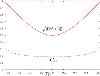
with $\rho_{diag}$ being the density matrix obtained by setting the off-diagonal elements of $\rho$ to zero and $S(x)=-\mathrm{Tr}(x\log_{2}x)$ is von Neumann’s entropy. Using the additivity of von Neumann’s entropy under tensor products, i.e., $S(x\otimes x)=2S(x)$ and the fact that $(\rho\otimes\rho)_{diag}=\rho_{diag}\otimes\rho_{diag}$, we see that the REC is also additive under tensor products, i.e., $C_{re}(\rho\otimes\rho)=2C_{re}(\rho)$. So, we shall be able to change the REC of the two copies of $\rho$ only if we can change its own REC. An interesting result we report here in this direction is that, contrary to what happens with the HSC and L1C, we can modify the REC of a qubit by controlling its populations, a quantity usually considered to have a classical character. For a qubit state, $\rho_{qb}=2^{-1}(\Gamma_{0}+\langle\Gamma_{1}^{d}\rangle\Gamma_{1}^{d}+\langle\Gamma_{(1,2)}^{s}\rangle\Gamma_{(1,2)}^{s}+\langle\Gamma_{(1,2)}^{a}\rangle\Gamma_{(1,2)}^{a})$,

$$C_{re}(\rho_{qb})=-\sum_{j=1}^{2}\frac{1+(-1)^{\delta_{j2}}\langle\Gamma_{1}^{d}\rangle}{2}\log_{2}\frac{1+(-1)^{\delta_{j2}}\langle\Gamma_{1}^{d}\rangle}{2}+\sum_{j=1}^{2}\frac{1+(-1)^{\delta_{j2}}G}{2}\log_{2}\frac{1+(-1)^{\delta_{j2}}G}{2},$$ (26)

with $G^{2}=$$\langle\Gamma_{1}^{d}\rangle^{2}+C_{l_{1}}^{2}(\rho_{qb}).$ The form of the equation for $C_{re}(\rho_{qb})$ is an indicative that the term $\langle\Gamma_{1}^{d}\rangle$, related to the populations, does not cancel out. We verify that this is indeed the case via an example, which is shown in Fig. 1.

Figure 1: (color online) Relative entropy of coherence as a function of the qubit’s population-controlling parameter $\langle\Gamma_{1}^{d}\rangle$ for a fixed value of the $l_{1}$-norm coherence $C_{l_{1}}(\rho_{qb})=\sqrt{\langle\Gamma_{(1,2)}^{s}\rangle^{2}+\langle\Gamma_{(1,2)}^{a}\rangle^{2}}=\sqrt{0+1/4}.$ If we look at the Bloch’s sphere in the $\mathbb{R}^{3}$ space $(\langle\Gamma_{1}^{d}\rangle,\langle\Gamma_{(1,2)}^{s}\rangle,\langle\Gamma_{(1,2)}^{a}\rangle)$, a constant value of $C_{l_{1}}$ (or of $C_{hs}$) will be associated with points in the lateral surface of a cylinder of physical states within the sphere. In this cylinder, for $\langle\Gamma_{1}^{d}\rangle$ running from $-\sqrt{1-C_{l_{1}}^{2}}$ to $\sqrt{1-C_{l_{1}}^{2}}$, different values of $|\langle\Gamma_{1}^{d}\rangle|$ shall lead to different values of $C_{re}$. The uppermost and downmost circles of that cylinder surface touch the sphere surface, and in these circles lie pure states for which the Bloch’s vector norm, shown in the upper (red) curve, is equal to one.

IV Coherence dynamics under qutrit dephasing and dissipation

In this section, we study the dynamics of some coherence functions under decoherence. Once for one-qubit states the Hilbert-Schmidt coherence (HSC) and the $l_{1}$-norm coherence (L1C) are proportional, their dynamic behavior shall be equivalent in this physically meaningful kind of process. For instance, for a qubit the freezing conditions Maziero_NLQC ; Adesso_frozenC for $C_{hs}$ and for $C_{l_{1}}$ are the same. However, even in this simplest context, the dynamic behavior of relative entropy of coherence (REC) is qualitatively disparate from those of HSC and L1C. And this is due to the dependence of the first on the populations. On the other hand, already for qutrits the proportionality between $C_{hs}$ and $C_{l_{1}}$ does not hold in general. Here we have $C_{l_{1}}(\rho_{qt})=\sum_{k,l}\sqrt{\langle\Gamma_{(k,l)}^{s}\rangle^{2}+\langle\Gamma_{(k,l)}^{a}\rangle^{2}}$ with $1\leq k<l\leq 3$. So, we can warrant that $C_{l_{1}}\propto C_{hs}$ only if one single pair $(\langle\Gamma_{(k,l)}^{s}\rangle,\langle\Gamma_{(k,l)}^{a}\rangle)$ is non-null. In the following we shall regard the dynamics induced by qutrit phase damping (PD) and amplitude damping (AD) channels. The Kraus’ operators for these channels are (see e.g. Refs. Guo_qutrit ; Khan_qutrit and references therein):

$$K_{0}^{pd}=\sqrt{1-p}\mathbb{I}_{3}\mbox{ and }K_{j}^{pd}=\sqrt{p}|j\rangle\langle j|\mbox{ for }j=1,2,3,$$ (27)

$$K_{0}^{ad}=|1\rangle\langle 1|+\sqrt{1-p}(|2\rangle\langle 2|+|3\rangle\langle 3|)\mbox{, }K_{1}^{ad}=\sqrt{p}|1\rangle\langle 2|\mbox{, }K_{2}^{ad}=\sqrt{p}|1\rangle\langle 3|,$$ (28)

with $\mathbb{I}_{3}$ being the $3\mathrm{x}3$ identity matrix.

For a qutrit prepared in a general state and submitted to the action of the PD or AD channels, the states at parametrized time $p$ Soares-Pinto2011 , $\rho_{p}=\sum_{j}K_{j}\rho K_{j}^{\dagger}$, are given as follows:

$$\rho_{p}^{pd}=\begin{bmatrix}3^{-1}+(\langle\Gamma_{1}^{d}\rangle+\langle\Gamma_{2}^{d}\rangle)/2&q(\langle\Gamma_{(1,2)}^{s}\rangle-i\langle\Gamma_{(1,2)}^{a}\rangle)/2&q(\langle\Gamma_{(1,3)}^{s}\rangle-i\langle\Gamma_{(1,3)}^{a}\rangle)/2\\ q(\langle\Gamma_{(1,2)}^{s}\rangle+i\langle\Gamma_{(1,2)}^{a}\rangle)/2&3^{-1}-(\langle\Gamma_{1}^{d}\rangle-\langle\Gamma_{2}^{d}\rangle)/2&q(\langle\Gamma_{(2,3)}^{s}\rangle-i\langle\Gamma_{(2,3)}^{a}\rangle)/2\\ q(\langle\Gamma_{(1,3)}^{s}\rangle+i\langle\Gamma_{(1,3)}^{a}\rangle)/2&q(\langle\Gamma_{(2,3)}^{s}\rangle+i\langle\Gamma_{(2,3)}^{a}\rangle)/2&3^{-1}-\langle\Gamma_{2}^{d}\rangle\end{bmatrix},$$ (29)

$$\rho_{p}^{ad}=\begin{bmatrix}(1+2p)/3+q(\langle\Gamma_{1}^{d}\rangle+\langle\Gamma_{2}^{d}\rangle)/2&\sqrt{q}(\langle\Gamma_{(1,2)}^{s}\rangle-i\langle\Gamma_{(1,2)}^{a}\rangle)/2&\sqrt{q}(\langle\Gamma_{(1,3)}^{s}\rangle-i\langle\Gamma_{(1,3)}^{a}\rangle)/2\\ \sqrt{q}(\langle\Gamma_{(1,2)}^{s}\rangle+i\langle\Gamma_{(1,2)}^{a}\rangle)/2&q(3^{-1}-(\langle\Gamma_{1}^{d}\rangle-\langle\Gamma_{2}^{d}\rangle)/2)&q(\langle\Gamma_{(2,3)}^{s}\rangle-i\langle\Gamma_{(2,3)}^{a}\rangle)/2\\ \sqrt{q}(\langle\Gamma_{(1,3)}^{s}\rangle+i\langle\Gamma_{(1,3)}^{a}\rangle)/2&q(\langle\Gamma_{(2,3)}^{s}\rangle+i\langle\Gamma_{(2,3)}^{a}\rangle)/2&q(3^{-1}-\langle\Gamma_{2}^{d}\rangle)\end{bmatrix},$$ (30)

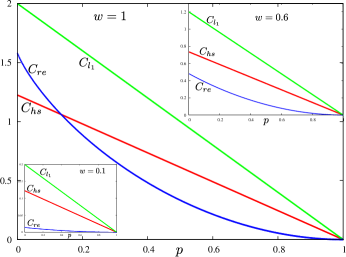
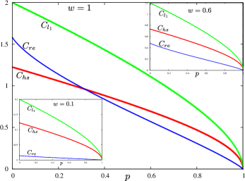
with $q=1-p$. As all off-diagonal elements of $\rho_{p}^{pd}$ decay at the same rate, we see that for the PD channel (PDC) the following motion equation holds for the L1C: $C_{l_{1}}(\rho_{p}^{pd})=(1-p)C_{l_{1}}(\rho^{pd})$. Besides, as all Bloch’s vector components from the symmetric and anti-symmetric sets are proportional to $1-p$, we get the following evolution equation for HSC: $C_{hs}(\rho_{p}^{pd})=(1-p)C_{hs}(\rho^{pd})$. Therefore, even if there is no simple-general proportionality relation between the initial values of L1C and HSC, the rate with which these values diminish with time for the PDC is once again observed to be equivalent. On the other hand, for this particular model of dissipation of three level systems, not all off-diagonal elements of $\rho_{p}^{ad}$ change equally with time. Here the time dependence of the coherences for the AD channel are:

$$C_{l_{1}}(\rho_{p}^{ad}) = \sqrt{1-p}\left(\sqrt{\langle\Gamma_{(1,2)}^{s}\rangle^{2}+\langle\Gamma_{(1,2)}^{a}\rangle^{2}}+\sqrt{\langle\Gamma_{(1,3)}^{s}\rangle^{2}+\langle\Gamma_{(1,3)}^{a}\rangle^{2}}\right)+(1-p)\sqrt{\langle\Gamma_{(2,3)}^{s}\rangle^{2}+\langle\Gamma_{(2,3)}^{a}\rangle^{2}},$$ (31)

$$C_{hs}(\rho_{p}^{ad}) = \frac{1}{\sqrt{2}}\sqrt{(1-p)\left(\langle\Gamma_{(1,2)}^{s}\rangle^{2}+\langle\Gamma_{(1,2)}^{a}\rangle^{2}+\langle\Gamma_{(1,3)}^{s}\rangle^{2}+\langle\Gamma_{(1,3)}^{a}\rangle^{2}\right)+(1-p)^{2}\left(\langle\Gamma_{(2,3)}^{s}\rangle^{2}+\langle\Gamma_{(2,3)}^{a}\rangle^{2}\right)}.$$ (32)

We illustrate the time dependence of these functions, and of REC, with the specific examples shown in Fig. 2.

Figure 2: (color online) Coherence of Hilbert-Schmidt (HSC), of the $l_{1}$-norm (L1C), and of the relative entropy (REC) under the action of the phase damping channel (plots on the left) and of the amplitude damping channel (plots on the right) for initial states $\rho_{w}=(1-w)\mathbb{I}_{3}/3+w|\psi\rangle\langle\psi|$ with $|\psi\rangle=3^{-1/2}\sum_{j=1}^{3}|j\rangle$. For these initial states, the dynamical behavior of HSC and L1C is seen to be similar, but quite different from that of the REC (regarding the functions concavities).

V Non-monotonicity of the HSD under tensor products

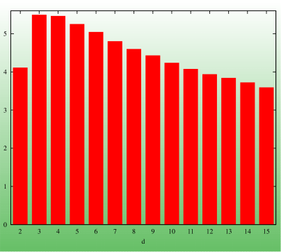
One can verify that, similarly to what happens with the trace distance (TD) Maziero_NMuTP , the Hilbert-Schmidt distance (HSD) does not suffer from the non-monotonicity under tensor product (NMuTP) issue for general pure states or for one-qubit collinear states. Actually, one can show that this holds true for all $p$-norm distances Ruskai . For general qudit states, the probability for random quartets of states to present the NMuTP behavior of HSD decays with increasing the system dimension, also similar to what was seen for the TD Maziero_NMuTP . For completeness, we show such probabilities in Fig. 3.

Regarding the Hilbert-Schmidt coherence (HSC), once

$$C_{hs}^{2}(\rho_{qb}\otimes\rho_{qb})=2C_{hs}^{2}(\rho_{qb})\left(1+C_{hs}^{2}(\rho_{qb})+\langle\Gamma_{1}^{d}\rangle_{\rho_{qb}}\right),$$ (33)

we see that the NMuTP behavior of the HSD can be revealed on its associated HSC if we manipulate $\langle\Gamma_{1}^{d}\rangle_{\rho_{qb}}$ accordingly; what we will do by using an example. We will consider $\langle\Gamma_{(1,2)}^{s}\rangle_{\rho_{qb}}=\langle\Gamma_{(1,2)}^{a}\rangle_{\rho_{qb}}=0.34$ and $\langle\Gamma_{(1,2)}^{s}\rangle_{\xi_{qb}}=\langle\Gamma_{(1,2)}^{a}\rangle_{\xi_{qb}}=0.33$, what gives us $C_{hs}(\rho_{qb})=0.34$ and $C_{hs}(\xi_{qb})=0.33,$ so

$$C_{hs}(\rho_{qb})>C_{hs}(\xi_{qb}).$$ (34)

In order to invert the dissimilarity relation, we fix $\langle\Gamma_{1}^{d}\rangle_{\rho_{qb}}=0$ and change $|\langle\Gamma_{1}^{d}\rangle_{\xi_{qb}}|$, which can vary from zero up to $\sqrt{1-2C_{hs}^{2}(\xi_{qb})}$. As $C_{hs}(\rho_{qb}\otimes\rho_{qb})\approx 0.26$, we can use e.g. $|\langle\Gamma_{1}^{d}\rangle_{\xi_{qb}}|=0.7$ to get $C_{hs}(\xi_{qb}\otimes\xi_{qb})\approx 0.39$, and consequently

$$C_{hs}(\rho_{qb}\otimes\rho_{qb})<C_{hs}(\xi_{qb}\otimes\xi_{qb}).$$ (35)

These last two inequalities are a manifestation of the NMuTP of HSD:

$$d(\rho,\iota_{\rho})>d(\xi,\iota_{\xi})\mbox{ and }d(\rho\otimes\rho,\iota_{\rho}\otimes\iota_{\rho})<d(\xi\otimes\xi,\iota_{\xi}\otimes\iota_{\xi}).$$ (36)

In the last equation we used the fact that, under the HSD, $\iota_{x\otimes x}=\iota_{x}\otimes\iota_{x}$.

Figure 3: (color online) Percentage of the random quartets of states leading to the non-monotonic behavior under tensor products of the Hilbert-Schmidt distance. Using the standard method from the library described in Ref. Maziero_LibForro (the associated Fortran code can be accessed freely in LibForro ), we generated one million quartets of states for each dimension $d$.

VI Concluding remarks

In this article, we started obtaining a closed formula for the Hilbert-Schmidt distance (HSD) between two generic $n$-qudit states in terms of the Euclidean distance between the corresponding rescaled Bloch’s vectors. We used this result to derive an analytical expression for the Hilbert-Schmidt quantum coherence (HSC) of $n$-qudit systems. This formula was then exemplified in simple cases and we applied it to investigated issues related to the distribution and transformation of quantum coherence in some composite systems.

After splitting the total HSC of two-qubit states into its local and non-local parts, we analyzed the possibility of controlling these coherences by tuning the local populations of two copies of a generic one-qubit state. Related to that matter, we observed some interesting contrasting behaviors of the HSC, $l_{1}$-norm coherence (L1C), and relative entropy of coherence (REC). We noticed that it is not possible to change the local HSC and L1C by tuning local populations. However, contrary the what was seen for the L1C, we can control the HSC by doing that kind of operation. The REC of two copies of a qubit state can be changed only if the local REC is changed, what we showed being possible by the control of local populations. This raises yet another bold difference among these coherence functions. In future works, it could be fruitful to investigate this kind of issue considering its possible physical implications and also another coherence quantifiers.

We also investigated the time evolution of coherence under qutrit dephasing and dissipation environments. The population-dependent character of the REC leads to its quite different dynamical behavior when compared to those of L1C and HSC. These last two coherence functions are seen to be equivalent for qubits and for some qutrit states. Besides, we have shown that even when HSC and L1C are not proportional, their dynamical behavior can be similar.

We have identified the first important implication of the non-monotonicity under tensor product (NMuTP) property of a quantum distance measure. We showed that the NMuTP of HSD, when applied to some states, can indicate that although a configuration $\rho_{qb}$ is more coherent than another state $\xi_{qb}$, two independent copies of the first state possess less HSC than two copies of the last. We emphasize that we succeeded in doing that at this moment mainly because we used the HSD. This unexpected result, obtained for the HSD, calls for further investigations of the NMuTP issue regarding other quantum distance measures and also considering other of its possible consequences.