One dimensional fractional order $TGV$: Gamma-convergence and bilevel training scheme

Abstract.

New fractional $r$-order seminorms, $TGV^{r}$, $r\in{\mathbb{R}}$, $r\geq 1$, are proposed in the one-dimensional (1D) setting, as a generalization of the integer order $TGV^{k}$-seminorms, $k\in\mathbb{N}$. The fractional $r$-order $TGV^{r}$-seminorms are shown to be intermediate between the integer order $TGV^{k}$-seminorms. A bilevel training scheme is proposed, where under a box constraint a simultaneous optimization with respect to parameters and order of derivation is performed. Existence of solutions to the bilevel training scheme is proved by $\Gamma$–convergence. Finally, the numerical landscape of the cost function associated to the bilevel training scheme is discussed for two numerical examples.

1. Introduction

In the last decades, Calculus of Variations and Partial Differential Equations (PDE) methods have proven to be very efficient in signal (1D) and image (2D) denoising problems. Signal (image) denoising consists, roughly speaking, in recovering a noise-free clean signal $u_{c}$ starting from a corrupted signal $u_{\eta}=u_{c}+\eta$, by filtering out the noise encoded by $\eta$. One of the most successful variational approach to signal (image) denoising (see, for example [35, 36, 37]) relies on the ROF total-variational functional

$$ROF(u):=\left\|u-u_{\eta}\right\|_{L^{2}(I)}^{2}+\alpha TV(u),$$ (1.1)

introduced in [35]. Here $I=(0,1)$ represents the domain of a one-dimensional image (a signal), $\alpha\in\mathbb{R}^{+}$, and $TV(u)=\left\lvert u^{\prime}\right\rvert_{\mathcal{M}_{b}(I)}$, stands for the total mass of the measure $u^{\prime}$ on $I$ (see [2, Definition 1.4]).

An important role in determining the reconstruction properties of the ROF functional is played by the parameter $\alpha$. Indeed, if $\alpha$ is too large, then the total variation of $u$ is too penalized and the image turns out to be over-smoothed, with a resulting loss of information on the internal edges of the picture. Conversely, if $\alpha$ is too small then the noise remains un-removed. The choice of the “best” parameter $\alpha$ then becomes an important task.

In [24] the authors proposed a training scheme $(\mathcal{B})$ relying on a bilevel learning optimization defined in machine learning, namely on a semi-supervised training scheme that optimally adapts itself to the given “perfect data” (see [13, 14, 26, 27, 39, 40]). This training scheme searches for the optimal $\alpha$ so that the recovered image $u_{\alpha}$, obtained as a minimizer of (1.1), optimizes the $L^{2}$-distance from the clean image ${u_{c}}$. An implementation of $(\mathcal{B})$ equipped with total variation is the following:

Level 1. $$\,\,\,\,\,\,\,\,\,\,\,\,\,\,\,\,\,\,\,\,\,\,\,\,\,\,\,\,\,\,\,\,\,\,\,\,\,\alpha_{m}\in\mathop{\rm arg\,min}\left\{\left\|u_{\alpha}-u_{c}\right\|_{L^{2}(I)}^{2}:\,\,\alpha>0\right\}$$ (1.2)

Level 2. $$\,\,\,\,\,\,\,\,\,\,\,\,\,\,\,\,\,\,\,\,\,\,\,\,\,\,\,\,\,\,\,\,\,\,\,\,\,u_{\alpha}:=\mathop{\rm arg\,min}\left\{\left\|u-u_{\eta}\right\|_{L^{2}(I)}^{2}+\alpha TV(u):\,\,u\in SBV(I)\right\},$$ (1.3)

where $SBV(I)$ denotes the set of special functions of bounded variation in $I$ (see, e.g. [2, Chapter 4]).

It is well known that the ROF model in (1.1) suffers drawbacks like the staircasing effect, and the training scheme $(\mathcal{B})$ inherits that feature, namely the optimized reconstruction function $u_{\alpha_{m}}$ also exhibits the staircasing effect. One approach to counteract this problem is to insert higher-order derivatives in the regularizer (see [9, 11, 16, 33]). Two of the most successful image-reconstruction functionals among those involving mixed first and higher order terms are the infimal-convolution total variation ($ICTV$) [9] and the total generalized variation ($TGV$) models [33]. Note that they coincide with each other in the one-dimensional setting.

For $I:=(0,1)\subset{\mathbb{R}}$, $u\in BV(I)$, $k\in\mathbb{N}$, and $\alpha=(\alpha_{0},\dots,\alpha_{k})\in{\mathbb{R}}^{k+1}_{+}$, the $TGV^{k}_{\alpha}$ regularizer (see [43]) is defined as

$$\left\lvert u\right\rvert_{TGV^{1}_{\alpha}(I)}:=\alpha_{0}TV(u),$$ (1.4)

and

$$\left\lvert u\right\rvert_{TGV_{{\alpha}}^{k+1}(I)}:=\inf \left\{\alpha_{0}\left\lvert u^{\prime}-v_{0}\right\rvert_{\mathcal{M}_{b}(I)}+\alpha_{1}\left\lvert v_{0}^{\prime}-v_{1}\right\rvert_{{\mathcal{M}_{b}(I)}}+\right.$$

$$\qquad\left.\dots+\alpha_{k-1}\left\lvert v_{k-2}^{\prime}-v_{k-1}\right\rvert_{{\mathcal{M}_{b}(I)}}+\alpha_{k}\left\lvert v^{\prime}_{k-1}\right\rvert_{{\mathcal{M}_{b}(I)}}:\right.$$

$$\qquad\left.v_{i}\in BV(I)\text{ for }0\leq i\leq k-1\right\}.$$

For instance, for $k=1$, the $TGV^{2}_{\alpha_{0},\alpha_{1}}$ regularizer reads as

$$\left\lvert u\right\rvert_{TGV_{\alpha_{0},\alpha_{1}}^{2}(I)}:=\inf\left\{\alpha_{0}\left\lvert u^{\prime}-v_{0}\right\rvert_{\mathcal{M}_{b}(I)}+\alpha_{1}\left\lvert v^{\prime}_{0}\right\rvert_{{\mathcal{M}_{b}(I)}},\,\,v_{0}\in BV(I)\right\}.$$

Substituting $TGV^{2}_{\alpha_{0},\alpha_{1}}$ into (1.3) provides a bilevel training scheme with $TGV$ image-reconstruction model. We recall that large values of $\alpha_{1}$ will yield regularized solutions that are close to $TV$-regularized reconstructions, and large values of $\alpha_{0}$ will result in $TV^{2}$-type solutions (see, e.g., [34]). The best choice of parameters $\alpha_{0}$ and $\alpha_{1}$ is determined by an adaptation of the training scheme $(\mathcal{B})$ above (see [22] for a detailed study).

In the existing literature a regularizer is fixed a priori, and the biggest effort is concentrated on studying how to identify the best parameters. In the case of the $TGV^{k}$-model, this amounts to set manually the value of $k$ first, and then determine the optimal $\alpha_{m}$ in (1.3). However, there is no evidence suggesting that $TGV^{2}$ will always perform better than $TV$. In addition, the higher order seminorms $TGV^{k}$, $k\geq 2$, have rarely been analyzed, and hence their performance is largely unknown. Numerical simulations show that for different images (signals in 1D), different orders of $TGV^{k}$ might give different results. The main focus of this paper is exactly to investigate how to optimally tune both the weight $\alpha$ and the order $k$ of the $TGV^{k}_{{\alpha}}$-seminorm, in order to achieve the best reconstructed image.

Our result is threefold. First, we develop a bilevel training scheme, not only for parameter training, but also for determining the optimal order $k$ of the regularizer $TGV^{k}$ for image reconstruction. A straightforward modification of $(\mathcal{B})$ would be to just insert the order of the regularizer inside the learning level 2 in (1.3). Namely,

Level 1. $$\,\,\,\,\,\,\,\,\,\,\,\,\,\,\,\,\,\,\,\,\,\,\,\,(\tilde{\alpha},\tilde{k}):=\mathop{\rm arg\,min}\left\{\left\|u_{\alpha,k}-u_{c}\right\|_{L^{2}(I)}^{2}:\,\,{\alpha}>0,\,\,k\in\mathbb{N}\right\}$$ (1.5)

Level 2. $$\,\,\,\,\,\,\,\,\,\,\,\,\,\,\,\,\,\,\,\,\,\,\,\,u_{{\alpha},k}:=\mathop{\rm arg\,min}\left\{\left\|u-u_{\eta}\right\|_{L^{2}(I)}^{2}+\left\lvert u\right\rvert_{TGV_{{\alpha}}^{k}(I)}:\,\,u\in SBV(I)\right\}.$$ (1.6)

Often, in order to show the existence of a solution of the training scheme and also for the numerical realization of the model, a box constraint

$$(\alpha,k)\in[\mathrm{P},\mathrm{1/P}]^{k+1}\times[1,\mathrm{1/P}],$$ (1.7)

where $P\in(0,1)$ small is a fixed real number, needs to be imposed (see, e.g. [3, 20]). However, such constraint makes the above training scheme less interesting. To be precise, restricting the analysis to the case in which $k\in\mathbb{N}$ is an integer, the box constraint (1.7) would only allow $k$ to take finitely many values, and hence the optimal order $\tilde{k}$ of the regularizer would simply be determined by performing scheme $(\mathcal{B})$ finitely many times, at each time with different values of $k$. In addition, finer texture effects, for which an “intermediate” reconstruction between the one provided by $TGV^{k}$ and $TGV^{k+1}$ for some $k\in\mathbb{N}$ would be needed, might be neglected in the optimization procedure.

Therefore, a main challenge in the setup of such a training scheme is to give a meaningful interpolation between the spaces $TGV^{k}$ and $TGV^{k+1}$, and hence to guarantee that the collection of such spaces itself exhibits certain compactness and lower semicontinuity properties. To this purpose, we modify the definition of the $TGV^{k}$ functionals by incorporating the theory of fractional Sobolev spaces, and we introduce the notion of fractional order $TGV^{k+s}$ spaces (see Definition 3.1), where $k\in\mathbb{N}$, and $0<s<1$. For $k=1$, our definition reads as follows.

$$\left\lvert u\right\rvert_{TGV_{\alpha}^{1+s}(I)}:=\inf\left\{\alpha_{0}\left\lvert u^{\prime}-sv_{0}\right\rvert_{\mathcal{M}_{b}(I)}+\alpha_{1}{s(1-s)}\left\lvert v_{0}\right\rvert_{W^{s,1+s(1-s)}(I)}\right.\\ \left.+\alpha_{0}s(1-s)\Big{|}\int_{I}v_{0}(x)\,dx\Big{|}:\,v_{0}\in W^{s,1+s(1-s)}(I)\right\}.$$

In the expression above, $W^{s,1+s(1-s)}(I)$ is the fractional Sobolev space of order $s$ and integrability $1+s(1-s)$. For every $k\in{\mathbb{N}}$ and $s\in[0,1]$ we additionally introduce the sets

$$BGV_{\alpha}^{k+s}(I):=\left\{u\in L^{1}(I):\,\left\lvert u\right\rvert_{TGV_{\alpha}^{k+s}(I)}<+\infty\right\},$$ (1.8)

namely the classes of functions with bounded generalized total-variation seminorm.

In our first main result (see Theorem 3.2) we show that the $TGV^{1+s}$ seminorm is indeed intermediate between $TGV^{1}$ and $TGV^{2}$, i.e., we prove that, up to subsequences,

$$\lim_{s\nearrow 1}\left\lvert u\right\rvert_{TGV^{1+s}_{\alpha}(I)}=\left\lvert u\right\rvert_{TGV^{2}_{\alpha}(I)}\text{ and }\lim_{s\searrow 0}\left\lvert u\right\rvert_{TGV^{1+s}_{\alpha}(I)}=\alpha_{0}\left\lvert u^{\prime}\right\rvert_{\mathcal{M}_{b}(I)}.$$ (1.9)

Equation (1.9) shows that, for $s\nearrow 1$, the behavior of the $TGV^{1+s}$-seminorm is close to the one of the standard $TGV^{2}$-seminorm, whereas for $s\searrow 0$ it approaches the $TV$ functional. We additionally prove (see Corollary 3.5) that analogous results hold for higher order $TGV^{k+s}$-seminorms. We point out that working with such interpolation spaces has many advantages. Indeed, $TGV^{k+s}$ is expected to inherit the properties of fractional order derivatives, which have shown to be able to reduce the staircasing and contrast effects in noise-removal problems (see, e.g. [12]).

Our second and third main results (Theorems 4.2 and 5.2) concern the following improved training scheme $(\mathcal{R})$, which, under the box constraint (1.7), simultaneously optimizes both the parameter $\alpha$ and the order $r$ of derivation:

Level 1. $$\,\,\,\,\,\,\,\,\,\,\,\,\,\,(\tilde{\alpha},\tilde{r}):=\mathop{\rm arg\,min}\left\{\left\|u_{\alpha,r}-u_{c}\right\|_{L^{2}(I)}^{2},\,\,(\alpha,r)\in[\mathrm{P},\mathrm{1/P}]^{{\lfloor r\rfloor}+1}\times[1,\mathrm{1/P}]\right\},$$ (1.10)

Level 2. $$\,\,\,\,\,\,\,\,\,\,\,\,\,\,u_{{\alpha},r}:=\mathop{\rm arg\,min}\left\{\left\|u-u_{\eta}\right\|_{L^{2}(I)}^{2}+TGV_{\alpha}^{r}(u):\,\,u\in BGV_{\alpha}^{r}(I)\right\}.$$ (1.11)

In the definition above, ${\lfloor r\rfloor}$ denotes the largest integer strictly smaller than or equal to $r$.

We first show in Theorem 4.2 that the fractional order $TGV^{r}_{\alpha}$ functionals

$$\mathcal{F}^{r}_{\alpha}(u):=\left\|u-u_{\eta}\right\|_{L^{2}(I)}^{2}+TGV_{\alpha}^{r}(u)\quad\text{for every }u\in BGV_{\alpha}^{r}(I)$$ (1.12)

are continuous, in the sense of $\Gamma$-convergence in the weak* topology of $BV(I)$ (see [7] and [15]), with respect to the parameters $\alpha$ and the order $r$. Secondly, in Theorem 5.2 we exploit this $\Gamma$-convergence result, to prove existence of solutions to our training scheme $(\mathcal{R})$. Note that, according to the given noisy image $u_{\eta}$ and noise-free image $u_{c}$, the Level 1 in our training scheme $(\mathcal{R})$ provides simultaneously an optimal regularizer $TGV^{\tilde{r}}$ and a corresponding optimal parameter $\tilde{\alpha}\in[\mathrm{P},\mathrm{1/P}]^{{\lfloor\tilde{r}\rfloor}+1}$. We point out that, in general, the optimal order of derivation $\tilde{r}$ might, or might not, be an integer. In other words, the fractional $TGV^{r}$ seminorms are not intended as an improvement but rather as an extension of the integer order $TGV^{k}$ seminorms, which for some classes of signals might provide optimal reconstruction and be selected by the bilevel training scheme.

Although this paper mainly focuses on a theoretical analysis of $TGV^{r}$ and on showing the existence of optimal results for the training scheme $(\mathcal{R})$, in Section 6 some preliminary numerical examples are discussed (see Figures 1–2). We stress that a complete description of the optimality conditions and a reliable numerical scheme for identifying the optimal solution of the training scheme (1.10) are beyond the scope of this work, and are still a challenging open problem. We refer to [21, 23] for some preliminary results in this direction. The two-dimensional setting of fractional order $TGV^{r}$ and $ICTV^{r}$ seminorms, as well as more extensive numerical analysis and examples for different type of images (with large flat areas, fine details, etc.), will be the subject of the follow-up work [18].

Our paper is organized as follows. In Section 2 we review the definitions and some basic properties of fractional Sobolev spaces. In Section 3 we introduce the fractional order $TGV^{r}$ seminorms, we study their main properties, and prove that they are intermediate between integer-order seminorms (see Theorem 3.2). In Section 4 we characterize the asymptotic behavior of the functionals $\mathcal{F}^{r}_{\alpha}$ with respect to parameters and order of derivations (see Theorem 4.2). In Section 5 we introduce our training scheme $(\mathcal{R})$. In particular, in Theorem 5.2 we show that $(\mathcal{R})$ admits a solution under the box constraint (1.7). Lastly, in Section 6 some examples and insights are provided.

2. The theory of fractional Sobolev Spaces

In what follows we will assume that $I=(0,1)$. We first recall a few results from the theory of fractional Sobolev spaces. We refer to [25] for an introduction to the main results, and to [1, 29, 30, 32] and the references therein for a comprehensive treatment of the topic.

Definition 2.1 (Fractional Sobolev spaces).

For $0<s<1$, $1\leq p<+\infty$, and $u\in L^{p}(I)$, we define the Gagliardo seminorm of $u$ by

$$\left\lvert u\right\rvert_{W^{s,p}(I)}:=\left(\int_{I}\int_{I}\frac{\left\lvert u(x)-u(y)\right\rvert^{p}}{|x-y|^{1+sp}}\,dx\,dy\right)^{\frac{1}{p}}.$$ (2.1)

We say that $u\in W^{s,p}(I)$ if

$$\left\|u\right\|_{W^{s,p}(I)}:=\left\|u\right\|_{L^{p}(I)}+\left\lvert u\right\rvert_{W^{s,p}(I)}<+\infty.$$ (2.2)

The following embedding results hold true ([25, Theorems 6.7, 6.10, and 8.2, and Corollary 7.2]).

Theorem 2.2 (Sobolev Embeddings - 1).

Let $s\in(0,1)$ be given.

1. Let $p<\frac{1}{s}$. Then there exists a positive constant $C=C(p,s)$ such that for every $u\in W^{s,p}(I)$ there holds

   $$\|u\|_{L^{q}(I)}\leq C\|u\|_{W^{s,p}(I)}$$ (2.3)

   for every $q\in[1,\tfrac{p}{1-sp}]$. If $q<\tfrac{p}{1-sp}$, then the embedding of $W^{s,p}(I)$ into $L^{q}(I)$ is also compact.

2. Let $p=\frac{1}{s}$. Then the embedding in (2.3) holds for every $q\in[1,+\infty).$

3. Let $p>\frac{1}{s}$. Then there exists a positive constant $C=C(p,s)$ such that for every $u\in W^{s,p}(I)$ we have

   $$\|u\|_{\mathcal{C}^{0,\alpha}(I)}\leq C\|u\|_{W^{s,p}(I)},$$

   with $\alpha:=\frac{sp-1}{p}$, where

   $$\left\|u\right\|_{\mathcal{C}^{0,\alpha}(I)}:=\|u\|_{L^{\infty}(I)}+\sup_{x\neq y\in I}\frac{|u(x)-u(y)|}{|x-y|^{\alpha}}.$$ (2.4)

The additional embedding result below is proved in [38, Corollary 19].

Theorem 2.3 (Sobolev Embeddings - 2).

Let $s\geq r$, $p\leq q$ and $s-1/p\geq r-1/q$, with $0<r\leq s<1$, and $1\leq p\leq q\leq+\infty$. Then

$$W^{s,p}(I)\subset W^{r,q}(I),$$ (2.5)

and

$$\left\lvert u\right\rvert_{W^{r,q}(I)}\leq\frac{36}{rs}\left\lvert u\right\rvert_{W^{s,p}(I)}.$$

The next inequality is a special case of [4, Theorem 1] and [31, Theorem 1].

Theorem 2.4 (Poincaré Inequality).

Let $p\geq 1$, and let $sp<1$. There exists a constant $C>0$ such that

$$\left\|u-\int_{I}u(x)\,dx\right\|^{p}_{L^{\tfrac{p}{1-sp}}(I)}\leq\frac{Cs(1-s)}{(1-sp)^{p-1}}\left\lvert u\right\rvert^{p}_{W^{s,p}(I)}.$$ (2.6)

It is possible to construct a continuous extension operator from $W^{s,1}(I)$ to $W^{s,1}({\mathbb{R}})$ (see,e.g., [25, Theorem 5.4]).

Theorem 2.5 (Extension Operator).

Let $s\in(0,1)$, and let $1\leq p<+\infty$. Then $W^{s,p}(I)$ is continuously embedded in $W^{s,p}({\mathbb{R}})$, namely there exists a constant $C=C(p,s)$ such that for every $u\in W^{s,p}(I)$ there exists $\tilde{u}\in W^{s,p}({\mathbb{R}})$ satisfying $\tilde{u}|_{I}=u$ and

$$\left\|\tilde{u}\right\|_{W^{s,p}({\mathbb{R}})}\leq C\left\|u\right\|_{W^{s,p}(I)}.$$ (2.7)

The next two theorems ([41, Section $2.2.2$, Remark 3, and Section $2.11.2$]) yield an identification between fractional Sobolev spaces and Besov spaces in ${\mathbb{R}}$, and guarantee the reflexivity of Besov spaces $B^{s}_{p,q}$ for $p,q$ finite.

Theorem 2.6 (Identification with Besov spaces).

If $1\leq p<+\infty$ and $s\in{\mathbb{R}}^{+}\setminus\mathbb{N}$, then

$$W^{s,p}({\mathbb{R}})=B^{s}_{p,p}({\mathbb{R}})$$ (2.8)

Theorem 2.7 (Reflexivity of Besov spaces).

Let $-\infty<s<+\infty$, $1\leq p<+\infty$ and $0<q<+\infty$. Then

$$(B^{s}_{p,q}({\mathbb{R}}))^{\prime}=B^{-s}_{p^{\prime},q^{\prime}}({\mathbb{R}}),$$ (2.9)

where $(B^{s}_{p,q}({\mathbb{R}}))^{\prime}$ is the dual of the Besov space $B^{s}_{p,q}({\mathbb{R}})$, and where $p^{\prime}$ and $q^{\prime}$ are the conjugate exponent of $p$ and $q$, respectively.

In view of Theorems 2.6 and 2.7 the following characterization holds true.

Corollary 2.8 (Reflexivity of fractional Sobolev spaces).

Let $1<p<+\infty$ and $s\in{\mathbb{R}}^{+}\setminus\mathbb{N}$. Then the fractional Sobolev space $W^{s,p}({\mathbb{R}})$ is reflexive.

We conclude this section by recalling two theorems describing the limit behavior of the Gagliardo seminorm as $s\nearrow 1$ and $s\searrow 0$, respectively. The first result has been proved in [5, Theorem 3 and Remark 1], and [17, Theorem 1].

Theorem 2.9 (Asymptotic behavior as $s\nearrow 1$).

Let $u\in BV(I)$. Then

$$\lim_{s\nearrow 1}(1-s)\left\lvert u\right\rvert_{W^{s,1}(I)}=|u^{\prime}|_{{\mathcal{M}_{b}(I)}}.$$

Similarly, the asymptotic behavior of the Gagliardo seminorm has been characterized as $s\searrow 0$ in [31, Theorem 3].

Theorem 2.10 (Asymptotic behavior as $s\searrow 0$).

Let $u\in\cup_{0<s<1}W^{s,1}({\mathbb{R}})$. Then,

$$\lim_{s\searrow 0}s\left\lvert u\right\rvert_{W^{s,1}({\mathbb{R}})}=4\left\|u\right\|_{L^{1}({\mathbb{R}})}.$$

3. The Fractional order $TGV$ seminorms

Let $r\in(1,+\infty)\setminus{\mathbb{N}}$ be given. In this section we define the fractional $r$-order total generalized variation ($TGV^{r}$) seminorms, and we prove some first properties.

Definition 3.1 (The $TGV^{r}$ seminorms).

Let $0<s<1$, $k\in\mathbb{N}$ be such that $k+s=r$, and let $\alpha=(\alpha_{0},\alpha_{1},\alpha_{2},\ldots,\alpha_{k})\in{\mathbb{R}}_{+}^{k+1}$. For every $u\in L^{1}(I)$, we define its fractional $TGV^{k+s}$ seminorm as follows.

1. for $k=1$

   $$\left\lvert u\right\rvert_{TGV_{\alpha}^{1+s}(I)}:=\inf\left\{\alpha_{0}\left\lvert u^{\prime}-sv_{0}\right\rvert_{\mathcal{M}_{b}(I)}+\alpha_{1}{s(1-s)}\left\lvert v_{0}\right\rvert_{W^{s,1+s(1-s)}(I)}\right.\\ \left.+\alpha_{0}s(1-s)\left\lvert\int_{I}v_{0}(x)\,dx\right\rvert\color[rgb]{0,0,0}:\,v_{0}\in W^{s,1+s(1-s)}(I)\right\}.$$ (3.1)

2. for $k>1$

   $$\left\lvert u\right\rvert_{TGV_{\alpha}^{k+s}(I)}:=\inf \left\{\alpha_{0}\left\lvert u^{\prime}-v_{0}\right\rvert_{\mathcal{M}_{b}(I)}+\alpha_{1}\left\lvert v_{0}^{\prime}-v_{1}\right\rvert_{{\mathcal{M}_{b}(I)}}+\right.$$

   $$\left.\cdots+\alpha_{k-1}\left\lvert v_{k-2}^{\prime}-sv_{k-1}\right\rvert_{{\mathcal{M}_{b}(I)}}+\alpha_{k}{s(1-s)}\left\lvert v_{k-1}\right\rvert_{W^{s,1+s(1-s)}(I)}\right.$$

   $$\left.+\alpha_{k-1}s(1-s)\left\lvert\int_{I}v_{k-1}(x)\,dx\right\rvert:\right.$$

   $$\left.v_{i}\in BV(I)\text{ for }0\leq i\leq k-2,\,\,v_{k-1}\in W^{s,1+s(1-s)}(I).\color[rgb]{0,0,0}\right\}$$

Moreover, we say that $u$ belongs to the space of functions with bounded total generalized variation, and we write $u\in BGV_{\alpha}^{k+s}(I)$ if

$$\left\|u\right\|_{BGV_{\alpha}^{k+s}(I)}:=\left\|u\right\|_{L^{1}(I)}+\left\lvert u\right\rvert_{TGV_{\alpha}^{k+s}(I)}<+\infty,$$ (3.2)

where $0\leq s<1$, $k\in\mathbb{N}$, $\alpha=(\alpha_{0},\alpha_{1},\alpha_{2},\ldots,\alpha_{k})\in{\mathbb{R}}_{+}^{k+1}$. Additionally, we write $u\in BGV^{k+s}(I)$ if there exists $\alpha\in{\mathbb{R}}_{+}^{k+1}$ such that $u\in BGV_{\alpha}^{k+s}(I)$. Note that if $u\in BGV_{\alpha}^{k+s}(I)$ for some $\alpha\in{\mathbb{R}}_{+}^{k+1}$, then $u\in BGV_{\beta}^{k+s}(I)$ for every $\beta\in{\mathbb{R}}_{+}^{k+1}$.

We observe that the $TGV^{k+s}$ seminorm is actually “intermediate” between the $TGV^{k}$ seminorm and the $TGV^{k+1}$ seminorm. To be precise, we have the following identification.

Theorem 3.2 (Asymptotic behavior of the fractional $TGV$ seminorm-1).

For every $u\in BV(I)$, up to the extraction of a (non-relabeled) subsequence there holds

$$\lim_{s\nearrow 1}\left\lvert u\right\rvert_{TGV^{1+s}_{\alpha}(I)}=\left\lvert u\right\rvert_{TGV^{2}_{\alpha}(I)}\text{ and }\lim_{s\searrow 0}\left\lvert u\right\rvert_{TGV^{1+s}_{\alpha}(I)}=\alpha_{0}\left\lvert u^{\prime}\right\rvert_{\mathcal{M}_{b}(I)}.$$ (3.3)

Before proving Theorem 3.2 we state and prove an intermediate result that will be crucial in determining the asymptotic behavior of the $TGV^{1+s}$ seminorm as $s\nearrow 1$.

Proposition 3.3.

Let $u\in W^{1,\infty}(I)$. Then

$$\limsup_{s\nearrow 1}(1-s)\left\lvert u\right\rvert_{W^{s,1+s(1-s)}(I)}\leq|u^{\prime}|_{\mathcal{M}_{b}(I)}.$$ (3.4)

Proof.

Let $u\in W^{1,\infty}(I)$. Then there exists a constant $L>0$ such that

$$|u(x)-u(y)|\leq L|x-y|^{s}$$ (3.5)

for every $x,y\in I$ and every $s\in(0,1)$. Thus

$$\left\lvert u\right\rvert^{1+s(1-s)}_{W^{s,1+s(1-s)}(I)}=\int_{I}\int_{I}\frac{|u(x)-u(y)|^{1+s(1-s)}}{|x-y|^{1+s(1+s(1-s))}}\,dx\,dy$$

$$\quad\leq L^{s(1-s)}\int_{I}\int_{I}\frac{|x-y|^{s^{2}(1-s)}|u(x)-u(y)|}{|x-y|^{1+s(1+s(1-s))}}\,dx\,dy$$

$$\quad=L^{s(1-s)}\int_{I}\int_{I}\frac{|u(x)-u(y)|}{|x-y|^{1+s}}\,dx\,dy=L^{s(1-s)}\left\lvert u\right\rvert_{W^{s,1}(I)}.$$

This implies that

$$(1-s)\left\lvert u\right\rvert_{W^{s,1+s(1-s)}(I)}\leq(1-s)L^{\frac{s(1-s)}{1+s(1-s)}}\left\lvert u\right\rvert^{\frac{1}{1+s(1-s)}}_{W^{s,1}(I)}$$

$$\quad=L^{\frac{s(1-s)}{1+s(1-s)}}\Big{[}(1-s)\left\lvert u\right\rvert_{W^{s,1}(I)}\Big{]}^{\frac{1}{1+s(1-s)}}e^{\frac{s(1-s)\log{(1-s)}}{1+s(1-s)}}.$$

Therefore, by Theorem 2.9 we conclude that

$$\limsup_{s\nearrow 1}(1-s)\left\lvert u\right\rvert_{W^{s,1+s(1-s)}(I)}\leq\limsup_{s\nearrow 1}\Big{[}(1-s)\left\lvert u\right\rvert_{W^{s,1}(I)}\Big{]}^{\frac{1}{1+s(1-s)}}\leq\left\lvert u^{\prime}\right\rvert_{\mathcal{M}_{b}(I)}.\qed$$

A crucial ingredient in the proof of Theorem 3.2 is a compactness and lower-semicontinuity result for maps with uniformly weighted averages and $W^{s,1+s(1-s)}$-seminorms.

Proposition 3.4.

Let $\{s_{n}\}\subset(0,1)$ be such that $s_{n}\to\bar{s}$, with $\bar{s}\in(0,1]$. For every $n\in\mathbb{N}$ let $v_{n}\in W^{s_{n},1+s_{n}(1-s_{n})}(I)$ be such that

$$\sup_{n\geq 1}s_{n}(1-s_{n})\left\{\left\lvert v_{n}\right\rvert_{W^{s_{n},1+s_{n}(1-s_{n})}(I)}+\Big{|}\int_{I}v_{n}(x)\,dx\Big{|}\right\}<+\infty.$$ (3.6)

Then, for $\bar{s}\in(0,1)$, there exists $\bar{v}\in W^{\bar{s},1+\bar{s}(1-\bar{s})}(I)$ such that, up to the extraction of a (non-relabeled) subsequence,

$$v_{n}\to\bar{v}\quad\text{strongly in }L^{1}(I),$$ (3.7)

and

$$\liminf_{n\to\infty}s_{n}(1-s_{n})\left\lvert v_{n}\right\rvert_{W^{s_{n},1+s_{n}(1-s_{n})}(I)}\geq\bar{s}(1-\bar{s})\left\lvert\bar{v}\right\rvert_{W^{\bar{s},1+{\bar{s}}(1-{\bar{s}})}(I)}.$$ (3.8)

For $\bar{s}=1$, there exists $\bar{v}\in BV(I)$ such that, up to the extraction of a (non-relabeled) subsequence,

$$v_{n}-\int_{I}v_{n}(x)\,dx\to\bar{v}\quad\text{strongly in }L^{1}(I),$$ (3.9)

and

$$\liminf_{n\to\infty}s_{n}(1-s_{n})\left\lvert v_{n}\right\rvert_{W^{s_{n},1+s_{n}(1-s_{n})}(I)}\geq\left\lvert\bar{v}^{\prime}\right\rvert_{\mathcal{M}_{b}(I)}.$$ (3.10)

Proof.

We first observe that for $x$, $y\in I$, $1\leq p<+\infty$, and $s<t$, we have

$$\left\lvert x-y\right\rvert^{1+sp}>\left\lvert x-y\right\rvert^{1+tp}.$$ (3.11)

Hence, in view of (2.1) there holds

$$\left\lvert u\right\rvert_{W^{s,p}(I)}\leq\left\lvert u\right\rvert_{W^{t,p}(I)}$$

for every $u\in W^{t,p}(I)$.

Without loss of generality (and up to the extraction of a non-relabeled subsequence) we can assume that the sequences $\{s_{n}\}$ and $\{s_{n}(1-s_{n})\}$ converge monotonically to ${\bar{s}}$ and ${\bar{s}}(1-{\bar{s}})$, respectively. According to the value of ${\bar{s}}$ only 4 situations can arise:

1. $\tfrac{1}{2}\leq{\bar{s}}<1$: $s_{n}\searrow\bar{s}$ and $s_{n}(1-s_{n})\nearrow{\bar{s}}(1-{\bar{s}})$;

2. $0<{\bar{s}}<\tfrac{1}{2}$: $s_{n}\searrow\bar{s}$ and $s_{n}(1-s_{n})\searrow{\bar{s}}(1-{\bar{s}})$;

3. $\tfrac{1}{2}<{\bar{s}}\leq 1$: $s_{n}\nearrow\bar{s}$ and $s_{n}(1-s_{n})\searrow{\bar{s}}(1-{\bar{s}})$;

4. $0<{\bar{s}}\leq\tfrac{1}{2}$: $s_{n}\nearrow\bar{s}$ and $s_{n}(1-s_{n})\nearrow{\bar{s}}(1-{\bar{s}})$.

For convenience of the reader we subdivide the proof into three steps.

Step 1: We first consider Case 1. By (3.6) there exists a constant $C$ such that

$$\sup_{n\geq 1}\left\{\left\lvert v_{n}\right\rvert_{W^{s_{n},1+s_{n}(1-s_{n})}(I)}+\Big{|}\int_{I}v_{n}(x)\,dx\Big{|}\right\}\leq C.$$ (3.12)

We point out that the function $f:(0,1)\to{\mathbb{R}}$, defined as

$$f(x):=x-\frac{1}{1+x(1-x)}\quad\text{for every }x\in[0,1],$$ (3.13)

is strictly increasing on $[0,1]$. In particular, since $s_{n}\geq\bar{s}$, there holds $f(s_{n})\geq f(\bar{s})$, namely

$$s_{n}-\frac{1}{1+s_{n}(1-s_{n})}\geq\bar{s}-\frac{1}{1+\bar{s}(1-\bar{s})}.$$ (3.14)

By applying Theorem 2.3 with $s=s_{n}$, $r={\bar{s}}$, $p=1+s_{n}(1-s_{n})$, and $q=1+{\bar{s}}(1-{\bar{s}})$, we obtain that there exists a constant $C$ such that

$$\left\lvert v_{n}\right\rvert_{W^{{\bar{s}},1+{\bar{s}}(1-{\bar{s}})}(I)}\leq C\left\lvert v_{n}\right\rvert_{W^{s_{n},1+s_{n}(1-s_{n})}(I)}$$ (3.15)

for every $n\in{\mathbb{N}}$. The uniform bound (3.12) yields then that there exists a constant $C$ such that

$$\sup_{n\geq 1}\left\lvert v_{n}\right\rvert_{W^{{\bar{s}},1+{\bar{s}}(1-{\bar{s}})}(I)}\leq C.$$ (3.16)

In view of Theorem 2.4, Corollary 2.8, and estimates (3.12) and (3.16) there exists $\bar{v}\in W^{{\bar{s}},1+{\bar{s}}(1-{\bar{s}})}(I)$ such that, up to the extraction of a (non-relabeled) subsequence, we have

$$v_{n}\rightharpoonup\bar{v}\quad\text{weakly in }W^{{\bar{s}},1+{\bar{s}}(1-{\bar{s}})}(I).$$ (3.17)

Since ${\bar{s}}(1+{\bar{s}}(1-{\bar{s}}))<1$, and $1<\frac{1+{\bar{s}}(1-{\bar{s}})}{1-{\bar{s}}(1+{\bar{s}}(1-{\bar{s}}))}$, by Theorem 2.2 (1.), the embedding of $W^{{\bar{s}},1+{\bar{s}}(1-{\bar{s}})}(I)$ into $L^{1}(I)$ is compact. Property (3.7) follows then by (3.17).

By the lower semicontinuity of the $W^{{\bar{s}},1+{\bar{s}}(1-{\bar{s}})}(I)$ norm with respect to the weak convergence, and by (3.15) we deduce the inequality

$${\bar{s}}(1-{\bar{s}})\left\lvert\bar{v}\right\rvert_{W^{{\bar{s}},1+{\bar{s}}(1-{\bar{s}})}(I)} \leq\liminf_{n\to+\infty}{\bar{s}}(1-{\bar{s}})\left\lvert v_{n}\right\rvert_{W^{s_{n},1+s_{n}(1-s_{n})}(I)}$$

$$=\liminf_{n\to+\infty}s_{n}(1-s_{n})\left\lvert v_{n}\right\rvert_{W^{s_{n},1+s_{n}(1-s_{n})}(I)},$$

which in turn yields (3.8).

Step 2: Consider now Case 2. The function $g:(0,1)\to{\mathbb{R}}$, defined as

$$g(x):=\frac{1}{1+x(1-x)}\quad\text{for every }x\in(0,1),$$ (3.18)

is strictly decreasing in $(0,\tfrac{1}{2}]$. By the definition of the maps $f$ (defined in (3.13)) and $g$ there holds

$$g({\bar{s}})+f({\bar{s}})={\bar{s}}.$$ (3.19)

Therefore, by the monotonicity of $g$ in $(0,\tfrac{1}{2}]$ there exist $\frac{1}{2}>\hat{s}>\bar{s}$, and $\lambda\in(0,1)$, such that $g(\hat{s})+f(\bar{s})>\lambda\bar{s}$, namely

$$\bar{s}-\frac{1}{1+\bar{s}(1-\bar{s})}>\lambda\bar{s}-\frac{1}{1+\hat{s}(1-\hat{s})}.$$ (3.20)

By the monotonicity of $f$ on $[0,1]$, and the fact that $s_{n}\geq\bar{s}$ for every $n\in{\mathbb{N}}$, we have

$$s_{n}-\frac{1}{1+s_{n}(1-s_{n})}=f(s_{n})>f({\bar{s}})={\bar{s}}-\frac{1}{1+{\bar{s}}(1-{\bar{s}})}>\lambda\bar{s}-\frac{1}{1+\hat{s}(1-\hat{s})}.$$ (3.21)

By (3.6) there exists a constant $C$ such that

$$\sup_{n\geq 1}\left\{\left\lvert v_{n}\right\rvert_{W^{s_{n},1+s_{n}(1-s_{n})}(I)}+\Big{|}\int_{I}v_{n}(x)\,dx\Big{|}\right\}\leq C.$$ (3.22)

Since $\frac{1}{2}>\hat{s}>{\bar{s}}$, and $s_{n}(1-s_{n})\searrow{\bar{s}}(1-{\bar{s}})$, there exists $n_{0}\in{\mathbb{N}}$ such that

$$1+s_{n}(1-s_{n})<1+\hat{s}(1-\hat{s})\quad\text{for every }n\geq n_{0}.$$ (3.23)

Hence, choosing $s=s_{n}$, $r=\lambda{\bar{s}}$, $p=1+s_{n}(1-s_{n})$, and $q=1+\hat{s}(1-\hat{s})$ in Theorem 2.3, we deduce that there exists a constant $C$ such that

$$\left\lvert v_{n}\right\rvert_{W^{\lambda{\bar{s}},1+\hat{s}(1-\hat{s})}(I)}\leq C\left\lvert v_{n}\right\rvert_{W^{s_{n},1+s_{n}(1-s_{n})}(I)}$$ (3.24)

for every $n\geq n_{0}$. In particular, (3.6) yields the uniform bound

$$\sup_{n\geq 1}\left\lvert v_{n}\right\rvert_{W^{\lambda{\bar{s}},1+\hat{s}(1-\hat{s})}(I)}\leq C.$$ (3.25)

In view of Theorem 2.4, Corollary 2.8, and estimate (3.22) we deduce the existence of a map $\bar{v}$ such that, up to the extraction of a (non-relabeled) subsequence,

$$v_{n}\rightharpoonup\bar{v}\quad\text{weakly in }W^{\lambda{\bar{s}},1+\hat{s}(1-\hat{s})}(I).$$ (3.26)

Since $\lambda{\bar{s}}(1+\hat{s}(1-\hat{s}))<\hat{s}(1+\hat{s}(1-\hat{s}))<1$, and $1<\frac{1+\hat{s}(1-\hat{s})}{1-\lambda{\bar{s}}(1+\hat{s}(1-\hat{s}))}$, by Theorem 2.2 (1.) the space $W^{\lambda{\bar{s}},1+\hat{s}(1-\hat{s})}(I)$ embeds compactly into $L^{1}(I)$. Hence, the convergence in (3.26) holds also strongly in $L^{1}(I)$, and (3.7) follows. In particular, Fatou’s Lemma yields

$$\left\lvert v\right\rvert_{W^{{\bar{s}},1+{\bar{s}}(1-{\bar{s}})}(I)}^{1+{\bar{s}}(1-{\bar{s}})}\leq\liminf_{n_{k}\to+\infty}\left\lvert v_{n_{k}}\right\rvert_{W^{s_{n_{k}},1+s_{n_{k}}(1-s_{n_{k}})}(I)}^{1+s_{n_{k}}(1-s_{n_{k}})},$$ (3.27)

which in turn implies (3.8).

Step 3: We omit the proof of the result in Case 4, and in Case 3 for ${\bar{s}}<1$, as they follow from analogous arguments. Regarding Case 3 for ${\bar{s}}=1$, by Hölder inequality we have

$$\int_{I}\int_{I}\frac{|v_{n}(x)-v_{n}(y)|}{|x-y|^{1+\frac{s_{n}}{2-s_{n}}}}\,dx\,dy$$ (3.28)

$$\leq\left[\int_{I}\int_{I}\left(\frac{|v_{n}(x)-v_{n}(y)|}{|x-y|^{1+\frac{s_{n}}{2-s_{n}}}}\right)^{1+s_{n}(1-s_{n})}\,dx\,dy\right]^{\frac{1}{1+s_{n}(1-s_{n})}}$$ (3.29)

$$=\left[\int_{I}\int_{I}\frac{|v_{n}(x)-v_{n}(y)|^{1+s_{n}(1-s_{n})}}{|x-y|^{1+\frac{s_{n}}{2-s_{n}}+s_{n}(1-s_{n})+\frac{s_{n}^{2}}{2-s_{n}}(1-s_{n})}}\,dx\,dy\right]^{\frac{1}{1+s_{n}(1-s_{n})}}.$$ (3.30)

Now,

$$1+\frac{s_{n}}{2-s_{n}}+s_{n}(1-s_{n})+\frac{s_{n}^{2}}{2-s_{n}}(1-s_{n})<1+s_{n}+s_{n}^{2}(1-s_{n})$$ (3.31)

for $n$ big enough (because $s_{n}\nearrow 1$). Thus

$$\frac{1}{|x-y|^{1+\frac{s_{n}}{2-s_{n}}+s_{n}(1-s_{n})+\frac{s_{n}^{2}}{2-s_{n}}(1-s_{n})}}<\frac{1}{|x-y|^{1+s_{n}+s_{n}^{2}(1-s_{n})}}$$ (3.32)

for every $x,y\in I$, $x\neq y$, and by (3.30) we obtain

$$\left\lvert v_{n}\right\rvert_{W^{\frac{s_{n}}{2-s_{n}},1}(I)}\leq\left\lvert v_{n}\right\rvert_{W^{s_{n},1+s_{n}(1-s_{n})}(I)}^{\frac{1}{1+s_{n}(1-s_{n})}}$$ (3.33)

for every $n\in{\mathbb{N}}$. Property (3.6) yields the existence of a constant $C$ such that

$$\sup_{n\in{\mathbb{N}}}(1-s_{n})\Big{(}\left\lvert v_{n}\right\rvert_{W^{\frac{s_{n}}{2-s_{n}},1}(I)}+\Big{|}\int_{I}v_{n}(x)\,dx\Big{|}\Big{)}\leq C.$$ (3.34)

Setting $t_{n}:=\frac{s_{n}}{2-s_{n}}$, there holds $t_{n}\to 1$ as $n\to+\infty$, and (3.34) implies

$$\sup_{n\in{\mathbb{N}}}(1-t_{n})\left\{\left\lvert v_{n}\right\rvert_{W^{t_{n},1}(I)}+\Big{|}\int_{I}v_{n}(x)\,dx\Big{|}\right\}\leq C.$$ (3.35)

Properties (3.9) and (3.10) are then a consequence of [5, Theorem 4]. ∎

We now prove Theorem 3.2.

Proof of Theorem 3.2.

Fix $\varepsilon>0$. Let $v_{0}\in BV(I)$ be such that

$$\left\lvert u\right\rvert_{TGV^{2}_{\alpha}(I)}\geq\alpha_{0}\left\lvert u^{\prime}-v_{0}\right\rvert_{\mathcal{M}_{b}(I)}+\alpha_{1}|v_{0}^{\prime}|_{\mathcal{M}_{b}(I)}-\varepsilon.$$ (3.36)

Let $v_{0}^{k}\in W^{1,\infty}(I)$ satisfy

$$\left\lvert|(v_{0}^{k})^{\prime}|_{\mathcal{M}_{b}(I)}-|v_{0}^{\prime}|_{\mathcal{M}_{b}(I)}\right\rvert<\varepsilon,$$ (3.37)

and

$$\left\|v_{0}-v_{0}^{k}\right\|_{L^{1}(I)}<\varepsilon.$$ (3.38)

In view of Proposition 3.3 there holds

$$\limsup_{s\nearrow 1}\left\lvert u\right\rvert_{TGV^{1+s}_{\alpha}(I)} \leq\limsup_{s\nearrow 1}\left\{\alpha_{0}\left\lvert u^{\prime}-sv_{0}^{k}\right\rvert_{\mathcal{M}_{b}(I)}+\alpha_{0}s(1-s)\Big{|}\int_{I}v_{0}^{k}(x)\,dx\Big{|}\right.$$

$$\qquad\left.+\alpha_{1}s(1-s)\left\lvert v_{0}^{k}\right\rvert_{W^{s,1+s(1-s)}(I)}\right\}$$

$$\quad\leq\alpha_{0}\left\lvert u^{\prime}-v_{0}^{k}\right\rvert_{\mathcal{M}_{b}(I)}+\alpha_{1}\left\lvert(v_{0}^{k})^{\prime}\right\rvert_{\mathcal{M}_{b}(I)}$$

$$\quad\leq\alpha_{0}\left\lvert u^{\prime}-v_{0}\right\rvert_{\mathcal{M}_{b}(I)}+\alpha_{1}\left\lvert v_{0}^{\prime}\right\rvert_{\mathcal{M}_{b}(I)}+(\alpha_{0}+\alpha_{1})\varepsilon$$

$$\quad\leq\left\lvert u\right\rvert_{TGV^{2}_{\alpha}(I)}+(\alpha_{0}+\alpha_{1}+1)\varepsilon.$$

The arbitrariness of $\varepsilon$ yields

$$\limsup_{s\nearrow 1}\left\lvert u\right\rvert_{TGV^{1+s}_{\alpha}(I)}\leq\left\lvert u\right\rvert_{TGV^{2}_{\alpha}(I)}.$$ (3.39)

To prove the opposite inequality, for every $s\in(0,1)$ let $v_{0}^{s}\in W^{s,1+s(1-s)}(I)$ be such that

$$\alpha_{0}\left\lvert u^{\prime}-sv_{0}^{s}\right\rvert_{\mathcal{M}_{b}(I)}+\alpha_{1}s(1-s)\left\lvert v_{0}^{s}\right\rvert_{W^{s,1+s(1-s)}(I)}+\alpha_{0}s(1-s)\Big{|}\int_{I}v_{0}^{s}(x)\,dx\Big{|}$$

$$\quad\leq\left\lvert u\right\rvert_{TGV^{1+s}_{\alpha}(I)}+s.$$ (3.40)

In view of (3.39) and Proposition 3.4, there exists $\tilde{v}\in BV(I)$ such that, up to the extraction of a (non-relabeled) subsequence,

$$v_{0}^{s}-\int_{I}v_{0}^{s}(x)\,dx\to\tilde{v}\quad\text{strongly in }L^{1}(I),$$ (3.41)

as $s\to 1$, and

$$\lim_{s\nearrow 1}s(1-s)\left\lvert v_{0}^{s}\right\rvert_{W^{s,1+s(1-s)}(I)}\geq\left\lvert\tilde{v}^{\prime}\right\rvert_{\mathcal{M}_{b}(I)}.$$ (3.42)

Additionally, by (3.39) and (3.40) there holds

$$s\left\|v_{0}^{s}\right\|_{L^{1}(I)}\leq\left\lvert u^{\prime}\right\rvert_{\mathcal{M}_{b}(I)}+\left\|u^{\prime}-sv_{0}^{s}\right\|_{\mathcal{M}_{b}(I)}\leq\left\lvert u^{\prime}\right\rvert_{\mathcal{M}_{b}(I)}+\left\lvert u\right\rvert_{TGV^{1+s}_{\alpha}(I)}+s\leq C$$

for every $s\in(0,1)$. Thus, there exists a constant $C$ such that

$$\lim_{s\to 1}\int_{I}v_{0}^{s}(x)\,dx=C.$$ (3.43)

In particular, setting $v:=\tilde{v}+C$, by (3.41) and (3.42) there holds

$$v_{0}^{s}\to v\quad\text{strongly in }L^{1}(I),$$ (3.44)

and

$$\lim_{s\to 1}s(1-s)\left\lvert v_{0}^{s}\right\rvert_{W^{s,1+s(1-s)}(I)}\geq\left\lvert v^{\prime}\right\rvert_{\mathcal{M}_{b}(I)}.$$ (3.45)

Passing to the limit in (3.40) we deduce the inequality

$$\left\lvert u\right\rvert_{TGV^{2}_{\alpha}(I)}\leq\alpha_{0}\left\lvert u^{\prime}-v\right\rvert_{\mathcal{M}_{b}(I)}+\alpha_{1}\left\lvert v^{\prime}\right\rvert_{\mathcal{M}_{b}(I)}\leq\liminf_{s\nearrow 1}\left\lvert u\right\rvert_{TGV^{1+s}_{\alpha}(I)},$$

which in turn implies the thesis.

To study the case $s\searrow 0$, we first observe that

$$\sup_{s\in(0,1)}\left\lvert u\right\rvert_{TGV^{1+s}_{\alpha}(I)}\leq\alpha_{0}\color[rgb]{0,0,0}|u^{\prime}|_{\mathcal{M}_{b}(I)}.$$ (3.46)

Thus we only need to prove the opposite inequality. To this aim, for every $s\in(0,1)$ let $v_{0}^{s}\in W^{s,1+s(1-s)}(I)$ be such that

$$\alpha_{0}\left\lvert u^{\prime}-sv_{0}^{s}\right\rvert_{\mathcal{M}_{b}(I)}+\alpha_{1}s(1-s)\left\lvert v_{0}^{s}\right\rvert_{W^{s,1+s(1-s)}(I)}+\alpha_{0}s(1-s)\Big{|}\int_{I}v_{0}^{s}(x)\,dx\Big{|}$$

$$\quad\leq\left\lvert u\right\rvert_{TGV^{1+s}_{\alpha}(I)}+s.$$ (3.47)

Since $s(1+s(1-s))<1$ for $s\in(0,1)$, by (3.46) and (3.47), and in view of Theorem 2.4, there exists a constant $C$ such that

$$s\int_{I}v_{0}^{s}(x)\,dx\to C,\quad\text{and}\quad sv_{0}^{s}\to C\quad\text{strongly in }L^{1}(I).$$ (3.48)

Passing to the limit in (3.47) we deduce the inequality

$$\alpha_{0}\left\lvert u^{\prime}\right\rvert_{\mathcal{M}_{b}(I)}\leq\alpha_{0}|u^{\prime}-C|_{\mathcal{M}_{b}(I)}+\alpha_{0}C\leq\liminf_{s\searrow 0}\left\lvert u\right\rvert_{TGV^{1+s}_{\alpha}(I)}.$$ (3.49)

The thesis follows owing to (3.46). ∎

Corollary 3.5 (Asymptotic behavior of the fractional $TGV$ seminorm-2).

Let $k\geq 2$. For every $u\in BV(I)$, up to the extraction of a (non-relabeled) subsequence there holds

$$\lim_{s\nearrow 1}\left\lvert u\right\rvert_{TGV^{k+s}_{\alpha}(I)}=\left\lvert u\right\rvert_{TGV^{k+1}_{\alpha}(I)}\text{ and }\lim_{s\searrow 0}\left\lvert u\right\rvert_{TGV^{k+s}_{\alpha}(I)}=\left\lvert u\right\rvert_{TGV^{k}_{\hat{\alpha}}(I)},$$ (3.50)

where $\hat{\alpha}:=(\alpha_{0},\dots,\alpha_{k-1})\in{\mathbb{R}}^{k}_{+}$.

Proof.

The result follows by straightforward adaptations of the arguments in the proof of Theorem 3.2. ∎

We proceed by showing that the minimization problem in Definition 3.1 has a solution.

Proposition 3.6.

If the infimum in Definition 3.1 is finite, then it is attained.

Proof.

Let $k=1$. Let $\alpha\in\mathbb{R}^{2}_{+}$, and let $u\in BGV^{1+s}_{\alpha}(I)$. We need to show that

$$\left\lvert u\right\rvert_{TGV^{1+s}_{\alpha}(I)}=\min\left\{\alpha_{0}\left\lvert u^{\prime}-sv\right\rvert_{{\mathcal{M}_{b}(I)}}+\alpha_{1}s(1-s)\left\lvert v\right\rvert_{W^{s,1+s(1-s)}(I)}\right.\\ \left.+\alpha_{0}s(1-s)\Big{|}\int_{I}v(x)\,dx\Big{|}\color[rgb]{0,0,0}:\,v\in W^{s,1+s(1-s)}(I)\right\}.$$ (3.51)

We first observe that $u\in BV(I)$.

Indeed, let $\delta>0$, and let $v\in W^{s,1+s(1-s)}(I)$ be such that

$$\alpha_{0}\left\lvert u^{\prime}-sv\right\rvert_{{\mathcal{M}_{b}(I)}}+\alpha_{1}s(1-s)\left\lvert v\right\rvert_{W^{s,1+s(1-s)}(I)}+\alpha_{0}s(1-s)\Big{|}\int_{I}v(x)\,dx\Big{|}\leq\left\lvert u\right\rvert_{TGV^{1+s}_{\alpha}(I)}+\delta.$$ (3.52)

By Hölder inequality there holds

$$\alpha_{0}\left\lvert u^{\prime}\right\rvert_{\mathcal{M}_{b}(I)}\leq\alpha_{0}\left\lvert u^{\prime}-sv\right\rvert_{\mathcal{M}_{b}(I)}+\alpha_{0}s\left\|v\right\|_{L^{1}(I)}$$

$$\leq\alpha_{0}\left\lvert u^{\prime}-sv\right\rvert_{\mathcal{M}_{b}(I)}+\alpha_{1}s\left\lvert v\right\rvert_{W^{s,1+s(1-s)}(I)}+\alpha_{0}s\left\|v\right\|_{L^{1+s(1-s)}(I)}+\alpha_{0}s(1-s)\Big{|}\int_{I}v(x)\,dx\Big{|}$$

$$\leq\left\lvert u\right\rvert_{TGV^{1+s}_{\alpha}(I)}+\delta+\alpha_{1}s^{2}\left\lvert v\right\rvert_{W^{s,1+s(1-s)}(I)}+\alpha_{0}s\left\|v\right\|_{L^{1+s(1-s)}(I)},$$

which implies the claim.

Let now $\left\{v_{n}\right\}\subset W^{s,1+s(1-s)}(I)$ be a minimizing sequence for (3.51). Since $s(1+s(1-s))<1$ for $s\in(0,1)$, by Theorem 2.2 (1.) there exists a constant $C$ such that

$$\sup_{n\in\mathbb{N}}\left\|v_{n}\right\|_{W^{s,1+s(1-s)}(I)}\leq C.$$ (3.53)

Thus, by Corollary 2.8 there exists $\bar{v}\in W^{s,1+s(1-s)}(I)$ such that, up to the extraction of a (non-relabeled) subsequence, there holds

$$v_{n}\rightharpoonup\bar{v}\quad\text{weakly in }W^{s,1+s(1-s)}(I),$$ (3.54)

and hence by Theorem 2.2 (1.),

$$v_{n}\to\bar{v}\quad\text{strongly in }L^{1}(I).$$ (3.55)

The thesis follows now by the lower semicontinuity of the total variation and the $W^{s,1+s(1-s)}$-norm with respect to the $L^{1}$ convergence and the weak convergence in $W^{s,1+s(1-s)}(I)$, respectively.

For $k=2$, let $\left\{v_{0}^{n}\right\}\subset BV(I)$ and $\left\{v_{1}^{n}\right\}\subset W^{s,1+s(1-s)}(I)$ be such that

$$\lim_{n\to+\infty}\left\{\alpha_{0}|u^{\prime}-v_{0}^{n}|_{\mathcal{M}_{b}(I)}+\alpha_{1}|(v_{0}^{n})^{\prime}-sv_{1}^{n}|_{\mathcal{M}_{b}(I)}+\alpha_{2}s(1-s)|v_{1}^{n}|_{W^{s,1+s(1-s)}(I)}\right.$$

$$\quad\left.+\alpha_{0}s(1-s)\Big{|}\int_{I}v_{1}^{n}(x)\,dx\Big{|}\color[rgb]{0,0,0}\right\}=TGV^{2+s}_{\alpha}(I).$$

Since $s(1+s(1-s))<1$ for $s\in(0,1)$, by Theorem 2.2 (1.) we obtain that $\left\{v_{1}^{n}\right\}$ is uniformly bounded in $W^{s,1+s(1-s)}(I)$. Therefore, $\left\{v_{0}^{n}\right\}$ is uniformly bounded in $BV(I)$, and there exist $v_{0}\in BV(I)$ and $v_{1}\in W^{s,1+s(1-s)}(I)$ such that, up to the extraction of a (non-relabeled) subsequence,

$$v_{0}^{n}\mathrel{\mathop{\rightharpoonup}\limits^{*}}v_{0}\quad\text{weakly* in }BV(I),$$ (3.56)

and

$$v_{1}^{n}\rightharpoonup v_{1}\quad\text{weakly in }W^{s,1+s(1-s)}(I).$$ (3.57)

In particular, by Theorem 2.2 (1.),

$$v_{1}^{n}\to v_{1}\quad\text{strongly in }L^{1}(I).$$ (3.58)

The minimality of $v_{0}$ and $v_{1}$ is a consequence of lower semicontinuity. The thesis for $k>2$ follows by analogous arguments. ∎

We observe that the $TGV^{k+s}$ seminorms are all topologically equivalent to the total variation seminorm.

Proposition 3.7.

For every $k\geq 1$ and $0<s<1$, we have

$$BV(I)\sim BGV^{k}(I)\sim BGV^{k+s}(I),$$ (3.59)

namely the three function spaces are topologically equivalent.

Proof.

We only show that

$$BV(I)\sim BGV^{1+s}(I)\sim BGV^{2}(I).$$ (3.60)

The proof of the inequality for $k>1$ is analogous. In view of (3.46), to prove the first equivalence relation in (3.60) we only need to show that there exist a constant $C$ and a multi-index $\alpha\in\mathbb{R}^{2}_{+}$ such that

$$\left\lvert u^{\prime}\right\rvert_{\mathcal{M}_{b}\left(I\right)}\leq C\left\lvert u\right\rvert_{TGV^{1+s}_{\alpha}(I)}.$$ (3.61)

By Theorem 2.2 we have

$$\left\lvert u^{\prime}\right\rvert_{\mathcal{M}_{b}(I)}\leq\left\lvert u^{\prime}-sv_{0}\right\rvert_{\mathcal{M}_{b}(I)}+s\left\|v_{0}\right\|_{L^{1}(I)}$$

$$\quad\leq\left\lvert u^{\prime}-sv_{0}\right\rvert_{\mathcal{M}_{b}(I)}+Cs\left\lvert v_{0}\right\rvert_{W^{s,1+s(1-s)}(I)}+s(1-s)\Big{|}\int_{I}v_{0}(x)\,dx\Big{|}$$

$$\quad=\left\lvert u^{\prime}-sv_{0}\right\rvert_{\mathcal{M}_{b}(I)}+\frac{C}{(1-s)}s(1-s)\left\lvert v_{0}\right\rvert_{W^{s,1+s(1-s)}(I)}+s(1-s)\Big{|}\int_{I}v_{0}(x)\,dx\Big{|}$$

for every $v_{0}\in W^{s,1+s(1-s)}(I)$. Thus

$$\left\lvert u^{\prime}\right\rvert_{\mathcal{M}_{b}(I)}\leq C\left\lvert u\right\rvert_{TGV^{1+s}_{1,\frac{C}{(1-s)}}(I)}$$ (3.62)

for every $s\in(0,1)$. This completes the proof of the first equivalence in (3.60). Property (3.60) follows now by [8, Theorem 3.3]. ∎

4. The fractional $r$-order $TGV^{r}$ functional

In this section we introduce the fractional $r$-order $TGV^{r}$ functional and prove a $\Gamma$-convergence result with respect to the parameters $\alpha$ and $s$.

Definition 4.1.

Let $r\in[1,+\infty)$, $\alpha\in{\mathbb{R}}^{\lfloor r\rfloor+1}_{+}$, and $u_{\eta}\in L^{2}(I)$. We define the functional $\mathcal{F}^{r}_{\alpha}:BV(I)\to[0,+\infty)$ as

$$\mathcal{F}^{r}_{\alpha}(u):=\int_{I}|u-u_{\eta}|^{2}\,dx+\left\lvert u\right\rvert_{TGV^{r}_{\alpha}(I)}$$ (4.1)

for every $u\in BV(I)$. Note that the definition is well-posed due to Proposition 3.7.

The main result of this section reads as follows.

Theorem 4.2 ($\Gamma$-convergence of the fractional order $TGV$ functional).

Let $k\in{\mathbb{N}}$ and $u_{\eta}\in L^{2}(I)$. Let $\{s_{n}\}\subset[0,1]$ and $\{\alpha_{n}\}\subset{\mathbb{R}}^{k+1}_{+}$ be such that $s_{n}\to s$, and $\alpha_{n}\to\alpha$. Then, if $s\in(0,1]$, the functional $\mathcal{F}^{k+s_{n}}_{\alpha_{n}}$ $\Gamma$-converges to $\mathcal{F}^{k+s}_{\alpha}$ in the weak* topology of $BV(I)$, namely for every $u\in BV(I)$ the following two conditions hold:

1. If

   $$u_{n}\mathrel{\mathop{\rightharpoonup}\limits^{*}}\text{weakly* in }BV(I),$$ (4.2)

   then

   $$\mathcal{F}^{k+s}_{\alpha}(u)\leq\liminf_{n\to+\infty}\mathcal{F}^{k+s_{n}}_{\alpha_{n}}(u_{n}).$$ (4.3)

2. There exists $\{u_{n}\}\subset BV(I)$ such that

   $$u_{n}\mathrel{\mathop{\rightharpoonup}\limits^{*}}u\quad\text{weakly* in }BV(I),$$ (4.4)

   and

   $$\limsup_{n\to+\infty}\mathcal{F}^{k+s_{n}}_{\alpha_{n}}(u_{n})\leq\mathcal{F}^{k+s}_{\alpha}(u).$$ (4.5)

The same result holds for $s=0$, by replacing $\alpha=(\alpha_{0},\dots,\alpha_{k})$ with $\hat{\alpha}:=(\alpha_{0},\dots,\alpha_{k-1})$ in (LI) and (RS).

Remark 4.3.

We recall that $\Gamma$-convergence is a variational convergence, originally introduced by E. De Giorgi and T. Franzoni in the seminar paper [19], which guarantees, roughly speaking, convergence of minimizers of the sequence of functionals to minimizers of the $\Gamma$-limit. The first condition in Theorem 4.2, known as liminf inequality ensures that the $\Gamma$-limit provides a lower bound for the asymptotic behavior of the $TGV^{k+s_{n}}_{\alpha_{n}}$ functionals, whereas the second condition, namely the existence of a recovery sequence guarantees that this lower bound is attained. We refer to [7] and [15] for a thorough discussion of the topic.

We subdivide the proof of Theorem 4.2 into two propositions. The next result will be crucial for establishing the liminf inequality.

Proposition 4.4.

Let $k\in{\mathbb{N}}$ and $u_{\eta}\in L^{2}(I)$. Let $\{s_{n}\}\subset[0,1]$ and $\{\alpha_{n}\}\subset{\mathbb{R}}^{k+1}_{+}$ be such that $s_{n}\to s$, and $\alpha_{n}\to\alpha$. Let $\{u_{n}\}\in BV(I)$ be such that

$$\sup_{n\in\mathbb{N}}\mathcal{F}^{k+s_{n}}_{\alpha_{n}}(u_{n})<+\infty.$$ (4.6)

Then, there exists $u\in BV(I)$ such that, up to the extraction of a (non-relabeled) subsequence, there holds

$$u_{n}\mathrel{\mathop{\rightharpoonup}\limits^{*}}u\text{ in }BV(I).$$ (4.7)

In addition, if $s\in(0,1]$ there holds

$$\left\lvert u\right\rvert_{TGV^{k+s}_{{\alpha}}(I)}\leq\liminf_{n\to+\infty}\left\lvert u_{n}\right\rvert_{TGV^{k+s_{n}}_{\alpha_{n}}(I)}.$$ (4.8)

If $s=0$ we have

$$\left\lvert u\right\rvert_{TGV^{k}_{\hat{\alpha}}(I)}\leq\liminf_{n\to+\infty}\left\lvert u_{n}\right\rvert_{TGV^{k+s_{n}}_{\alpha_{n}}(I)},$$ (4.9)

where $\hat{\alpha}\in{\mathbb{R}}^{k}_{+}$ is the multi-index $\hat{\alpha}:=(\alpha_{0},\dots,\alpha_{k-1})$.

Proof.

We prove the statement for $k=1$. The proof of the result for $k>1$ follows via straightforward modifications.

For $k=1$, we have $\left\{\alpha^{n}\right\}\subset{\mathbb{R}}^{2}$, and

$$\left(\alpha^{n}_{0},\alpha^{n}_{1}\right)\to\left(\alpha_{0},\alpha_{1}\right).$$ (4.10)

By Proposition 3.6 we deduce that there exists $v_{0}^{n}\in W^{s_{n},1+s_{n}(1-s_{n})}(I)$ such that

$$\left\lvert u_{n}\right\rvert_{TGV_{\alpha^{n}}^{1+s_{n}}(I)}=\alpha^{n}_{0}\left\lvert u^{\prime}_{n}-s_{n}v_{0}^{n}\right\rvert_{\mathcal{M}_{b}(I)}+\alpha^{n}_{1}s_{n}(1-s_{n})\left\lvert v_{0}^{n}\right\rvert_{W^{s_{n},1+s_{n}(1-s_{n})}(I)}\\ +\alpha_{0}^{n}s_{n}(1-s_{n})\Big{|}\int_{I}v_{0}^{n}(x)\,dx\Big{|}\color[rgb]{0,0,0}.$$ (4.11)

We preliminary observe that (4.6), (4.10), and (4.11) yield the existence of a constant $C$ such that

$$s_{n}(1-s_{n})\Big{(}\left\lvert v_{0}^{n}\right\rvert_{W^{s_{n},1+s_{n}(1-s_{n})}(I)}+\Big{|}\int_{I}v_{0}^{n}(x)\,dx\Big{|}\Big{)}+\left\lvert u_{n}^{\prime}-s_{n}v_{0}^{n}\right\rvert_{\mathcal{M}_{b}(I)}\leq C\left\lvert u_{n}\right\rvert_{TGV_{\alpha^{n}}^{k+s_{n}}(I)}\leq C$$ (4.12)

for every $n\in{\mathbb{N}}$. For convenience of the reader we subdivide the proof into three steps.

Step 1: Assume first that $s\in(0,1)$. By Proposition 3.4 there exists $v_{0}\in W^{s,1+s(1-s)}(I)$ such that

$$v_{0}^{n}\to v_{0}\quad\text{strongly in }L^{1}(I),$$ (4.13)

and

$$\liminf_{n\to\infty}s_{n}(1-s_{n})\left\lvert v_{0}^{n}\right\rvert_{W^{s_{n},1+s_{n}(1-s_{n})}(I)}\geq s(1-s)\left\lvert v_{0}\right\rvert_{W^{s,1+s(1-s)}(I)}.$$ (4.14)

By (4.6), (4.10), (4.11), and (4.13) there exists a constant $C$ such that

$$\left\lvert u^{\prime}_{n}\right\rvert_{\mathcal{M}_{b}(I)}\leq C,$$ (4.15)

and hence, again by (4.6),

$$\sup_{n\in\mathbb{N}}\left\|u_{n}\right\|_{BV(I)}\leq C\sup_{n\in\mathbb{N}}\left\|u_{n}\right\|_{BGV_{\alpha^{n}}^{1+s_{n}}(I)}<+\infty$$

which implies (4.7).

By (4.7), (4.11), (4.13), (4.14), and since $0<s<1$, there holds

$$\liminf_{n\to\infty}\left\lvert u_{n}\right\rvert_{TGV_{\alpha^{n}}^{1+s_{n}}(I)}\geq\liminf_{n\to\infty}\alpha^{n}_{0}\left\lvert u^{\prime}_{n}-s_{n}v_{0}^{n}\right\rvert_{\mathcal{M}_{b}(I)}$$

$$\qquad+\liminf_{n\to\infty}\alpha^{n}_{1}s_{n}(1-s_{n})\left\lvert v_{0}^{n}\right\rvert_{W^{s_{n},1+s_{n}(1-s_{n})}(I)}+\liminf_{n\to\infty}\alpha^{n}_{0}s_{n}(1-s_{n})\left\lvert\int_{I}v_{0}^{n}(x)\,dx\right\rvert$$

$$\quad\geq\alpha_{0}\left\lvert u^{\prime}-sv_{0}\right\rvert_{\mathcal{M}_{b}(I)}+\alpha_{1}s(1-s)\left\lvert v_{0}\right\rvert_{W^{s,1+s(1-s)}(I)}$$

$$\qquad+\alpha_{0}s(1-s)\left\lvert\int_{I}v_{0}(x)\,dx\right\rvert\geq\left\lvert u\right\rvert_{TGV_{\alpha}^{1+s}(I)},$$

where in the last inequality we used the definition of the $TGV_{\alpha}^{1+s}$-seminorm. In particular, we deduce (4.8).

Step 2: Consider now the case in which $s=1$. In view of Proposition 3.4, estimate (4.12) yields the existence of a map $\tilde{v}_{0}\in BV(I)$ such that

$$v_{0}^{n}-\int_{I}v_{0}^{n}(x)\,dx\to\tilde{v}_{0}\quad\text{strongly in }L^{1}(I)$$ (4.16)

and

$$\left\lvert\tilde{v}_{0}^{\prime}\right\rvert_{\mathcal{M}_{b}(I)}\leq\liminf_{n\to+\infty}s_{n}(1-s_{n})\left\lvert v_{0}^{n}\right\rvert_{W^{s_{n},1+s_{n}(1-s_{n})}(I)}.$$ (4.17)

On the other hand, by (4.12) there holds

$$\left\lvert u^{\prime}_{n}-s_{n}\int_{I}v_{0}^{n}(x)\,dx\right\rvert_{\mathcal{M}_{b}(I)}\leq\left\lvert u_{n}^{\prime}-s_{n}v_{0}^{n}\right\rvert_{\mathcal{M}_{b}(I)}+s_{n}\left\|v_{0}^{n}-\int_{I}v_{0}^{n}(x)\,dx\right\|_{L^{1}(I)}\leq C$$

for every $n\in N$. Thus, there exists $\tilde{u}\in BV(I)$ such that

$$u_{n}-u_{n}(0)-s_{n}\Big{(}\int_{I}v_{0}^{n}(x)\,dx\Big{)}x\mathrel{\mathop{\rightharpoonup}\limits^{*}}\tilde{u}\quad\text{weakly* in }BV(I).$$ (4.18)

By (4.6) and by Definition 3.1, we have

$$\sup_{n\geq 1}\left\|u_{n}\right\|_{L^{1}(I)}\leq C.$$ (4.19)

In view of (4.18), testing the map $u_{n}-u_{n}(0)-s_{n}\Big{(}\int_{I}v_{0}^{n}(x)\,dx\Big{)}x$ against the function $x-\frac{1}{2}$, we obtain that

$$\lim_{n\to+\infty}\int_{I}u_{n}(x)\left(x-\frac{1}{2}\right)\,dx+\frac{s_{n}}{6}\int_{I}v_{0}^{n}(x)\,dx=\int_{I}\tilde{u}(x)\left(x-\frac{1}{2}\right)\,dx.$$ (4.20)

Thus, by (4.19),

$$\frac{s_{n}}{6}\Big{|}\int_{I}v_{0}^{n}(x)\,dx\Big{|}\leq\left\lvert\int_{I}u_{n}(x)\left(x-\frac{1}{2}\right)\,dx+\frac{s_{n}}{6}\int_{I}v_{0}^{n}(x)\,dx\right\rvert+\frac{1}{2}\left\|u_{n}\right\|_{L^{1}(I)}\leq C$$ (4.21)

for every $n\in{\mathbb{N}}$. By combining (4.16), (4.17), (4.18), and (4.21) we deduce that there exists $v_{0}\in BV(I)$ such that

$$v_{0}^{n}\to v_{0}\quad\text{strongly in }L^{1}(I),$$ (4.22)

and

$$\left\lvert v_{0}^{\prime}\right\rvert_{\mathcal{M}_{b}(I)}\leq\liminf_{n\to+\infty}s_{n}(1-s_{n})\left\lvert v_{0}^{n}\right\rvert_{W^{s_{n},1+s_{n}(1-s_{n})}(I)}.$$ (4.23)

In particular, by combining (4.12), (4.22), and (4.23) we have that

$$\left\lvert u_{n}^{\prime}\right\rvert_{\mathcal{M}_{b}(I)}\leq C$$ (4.24)

for every $n\in{\mathbb{N}}$, which by (4.6) yields (4.7).

Step 3: Consider finally the case in which $s=0$. In view of (4.12), and by Theorem 2.4 there holds

$$\left\|v_{0}^{n}-\int_{I}v_{0}^{n}(x)\,dx\right\|_{L^{1}(I)}\leq C$$ (4.25)

for every $n\in{\mathbb{N}}$. On the other hand, (4.12) yields

$$s_{n}\Big{|}\int_{I}v_{0}^{n}(x)\,dx\Big{|}\leq C$$ (4.26)

for every $n\in{\mathbb{N}}$. Combining (4.25) and (4.26) we conclude that there exists a constant $\lambda\in{\mathbb{R}}$ such that, up to the extraction of a (non-relabeled) subsequence there holds

$$s_{n}v_{0}^{n}\to\lambda\quad\text{strongly in }L^{1}(I).$$ (4.27)

As a result, in view of (4.6), Definition 3.1, and (4.12) we deduce the existence of a map $u\in BV(I)$ such that, up to the extraction of a (non-relabeled) subsequence,

$$u_{n}\mathrel{\mathop{\rightharpoonup}\limits^{*}}u\quad\text{weakly* in }BV(I).$$ (4.28)

Hence, by (4.11), (4.27), and (4.28) we have

$$\liminf_{n\to\infty}\left\lvert u_{n}\right\rvert_{TGV_{\alpha^{n}}^{1+s_{n}}(I)}\geq\liminf_{n\to\infty}\alpha^{n}_{0}\left\lvert u^{\prime}_{n}-s_{n}v_{0}^{n}\right\rvert_{\mathcal{M}_{b}(I)}$$ (4.29)

$$+\liminf_{n\to\infty}\alpha^{n}_{1}s_{n}(1-s_{n})\left\lvert v_{0}^{n}\right\rvert_{W^{s_{n},1+s_{n}(1-s_{n})}(I)}+\liminf_{n\to\infty}\alpha^{n}_{0}s_{n}(1-s_{n})\left\lvert\int_{I}v_{0}^{n}(x)\,dx\right\rvert$$ (4.30)

$$\geq\alpha_{0}\left\lvert u^{\prime}-\lambda\right\rvert_{\mathcal{M}_{b}(I)}+\alpha_{0}|\lambda|\geq\alpha_{0}\left\lvert u^{\prime}\right\rvert_{\mathcal{M}_{b}(I)},$$ (4.31)

which in turn implies (4.9). This concludes the proof of the proposition. ∎

The following result is instrumental for the construction of a recovery sequence.

Proposition 4.5.

Let $k\in{\mathbb{N}}$ and $u_{\eta}\in L^{2}(I)$. Let $\{s_{n}\}\subset[0,1]$ and $\{\alpha_{n}\}\subset{\mathbb{R}}^{k+1}_{+}$ be such that $s_{n}\to s$, and $\alpha_{n}\to\alpha$. Let $u\in BV(I)$. Then, if $s\in(0,1]$ there holds

$$\lim_{n\rightarrow\infty}\left\lvert u\right\rvert_{TGV^{k+s_{n}}_{\alpha_{n}}(I)}=\left\lvert u\right\rvert_{TGV^{k+s}_{\alpha}(I)},$$ (4.32)

and if $s=0$,

$$\lim_{n\rightarrow\infty}\left\lvert u\right\rvert_{TGV^{k+s_{n}}_{\alpha_{n}}(I)}=\left\lvert u\right\rvert_{TGV^{k+s}_{\hat{\alpha}}(I)},$$ (4.33)

where $\hat{\alpha}\in{\mathbb{R}}^{k}_{+}$ is the multi-index $\hat{\alpha}:=(\alpha_{0},\dots,\alpha_{k-1})$.

Proof.

We prove the proposition for $k=1$. The thesis for $k>1$ can be proven by analogous arguments. The special cases $s=0$ and $s=1$ have already been analyzed in Theorem 3.2, in the situation in which $\alpha_{n}=\alpha$ for all $n\in{\mathbb{N}}$. The thesis for general sequences $\{\alpha_{n}\}$ follows by straightforward adaptations. Therefore, without loss of generality, we can assume that $s\in(0,1)$. As a consequence of Proposition 4.4 we immediately have that

$$\liminf_{n\to\infty}\left\lvert u\right\rvert_{TGV^{1+s_{n}}_{\alpha}(I)}\geq\left\lvert u\right\rvert_{TGV^{1+s}_{\alpha}(I)}.$$ (4.34)

To prove the opposite inequality, fix $\varepsilon>0$. By the definition of the $TGV^{1+s}_{\alpha}(I)$-seminorm, and in view of [25, Theorems 2.4 and 5.4], there exists $v_{0}\in C^{\infty}(I)\cap W^{s,1+s(1-s)}(I)$ such that

$$\left\lvert u\right\rvert_{TGV^{1+s}(I)}\geq\alpha_{0}{\left\lvert u^{\prime}-sv_{0}\right\rvert_{\mathcal{M}_{b}(I)}+\alpha_{1}{s(1-s)}\left\lvert v_{0}\right\rvert_{W^{s,1+s(1-s)}(I)}}+\alpha_{0}{s(1-s)}\left\lvert\int_{I}v_{0}(x)\,dx\right\rvert-\varepsilon.$$ (4.35)

In particular, there holds $v_{0}\in C^{\infty}(I)\cap W^{s_{n},1+s_{n}(1-s_{n})}(I)$ for every $n\in{\mathbb{N}}$. Hence

$$\left\lvert u\right\rvert_{TGV^{1+s_{n}}_{\alpha}(I)}\leq\alpha_{0}\left\lvert u^{\prime}-s_{n}v_{0}\right\rvert_{\mathcal{M}_{b}(I)}$$ (4.36)

$$\quad+\alpha_{1}{s_{n}(1-s_{n})}\left\lvert v_{0}\right\rvert_{W^{s_{n},1+s_{n}(1-s_{n})}(I)}+\alpha_{0}{s_{n}(1-s_{n})}\left\lvert\int_{I}v_{0}(x)\,dx\right\rvert,$$ (4.37)

for every $n\in{\mathbb{N}}$, and

$$\limsup_{n\to\infty}\left\lvert u\right\rvert_{TGV^{1+s_{n}}_{\alpha}(I)}\leq\left\lvert u\right\rvert_{TGV^{1+s}_{\alpha}(I)}+\varepsilon.$$ (4.38)

The thesis follows by the arbitrariness of $\varepsilon$, and by combining (4.34) and (4.38). ∎

We conclude this section by proving Theorem 4.2.

Proof of Theorem 4.2.

Property (LI) is a direct consequence of Proposition 4.4. Property (RS) follows by Proposition 4.5, choosing $u_{n}=u$ for every $n\in{\mathbb{N}}$. ∎

5. The bilevel training scheme equipped with $TGV^{r}$ regularizer

Let $r\in[1,+\infty)$ be given and recall ${\lfloor r\rfloor}$ denote the largest integer smaller than or equal to $r$. We propose the following training scheme $(\mathcal{R})$ which takes into account the order of derivation $r$ of the regularizer and the parameter $\alpha\in{\mathbb{R}}^{\lfloor r\rfloor+1}_{+}$ simultaneously. We restrict our analysis to the case in which $\alpha$ and $r$ satisfy the box constraint

$$(\alpha,r)\in[P,1/P]^{\lfloor r\rfloor+1}\times[1,1/P]$$ (5.1)

where $P\in(0,1)$ small is a fixed real number.

Our new training scheme $(\mathcal{R})$ is defined as follows:

Level 1. $$\,\,\,\,\,\,\,\,\,\,\,\,\,\,\,\,\,\,\,\,\,\,\,\,\,\,\,\,(\tilde{\alpha},\tilde{r}):=\mathop{\rm arg\,min}\left\{\mathcal{I}(\alpha,r),\,\,(\alpha,r)\in[P,1/P]^{\lfloor r\rfloor+1}\times[1,1/P]\right\},$$ (5.2)

Level 2. $$\,\,\,\,\,\,\,\,\,\,\,\,\,\,\,\,\,\,\,\,\,\,\,\,\,\,\,\,u_{{\alpha},r}:=\mathop{\rm arg\,min}\left\{\mathcal{F}^{r}_{\alpha}(u):\,\,{u\in BV(I)}\right\}$$ (5.3)

where $\mathcal{I}(\alpha,r)$, defined as

$$\mathcal{I}(\alpha,r):=\left\|u_{\alpha,r}-u_{c}\right\|_{L^{2}(I)}^{2}$$ (5.4)

is the cost function associated to the training scheme $(\mathcal{R})$, $\mathcal{F}^{r}_{\alpha}$ is introduced in Definition 4.1, the map $u_{c}\in L^{2}(I)$ represents a noise-free test signal, and $u_{\eta}\in L^{2}(I)$ is the noise (corrupted) signal.

Note that we only allow the parameters ${\alpha}$ and the order $r$ of regularizers to lie within a prescribed finite range. This is needed to force the optimal reconstructed signal $u_{\tilde{\alpha},\tilde{r}}$ to remain inside our proposed space $BV(I)$ (see Proposition 4.4). In particular, if some of the components of $\tilde{\alpha}$ blow up to $\infty$, we might end up in the space $W^{r,1}(I)$, which is outside the purview of this paper. We point out that $P$ can be chosen as small as the user wants. Thus, despite the box constraint, our analysis still incorporates a large class of regularizers, such as $TV$ and $TGV^{2}$ (see, e.g., [22]).

Before we state the main theorem of this section, we prove a technical lemma and show that (5.3) has a unique minimizer for each given $(\alpha,r)$.

Lemma 5.1.

For every $r\in[1,\mathrm{1/P}]$ and $\alpha\in{\mathbb{R}}^{\lfloor r\rfloor+1}_{+}$, there exists a unique $u_{\alpha,r}\in BV(I)$ solving the minimization problem (5.3).

Proof.

Let $\left\{u_{n}\right\}\subset BV(I)$ be a minimizing sequence for (5.3). By Proposition 3.7, $\left\{u_{n}\right\}$ is uniformly bounded in $BV(I)$. Thus there exists ${u}_{\alpha,r}\in BV(I)$ such that

$$u_{n}\mathrel{\mathop{\rightharpoonup}\limits^{*}}{u}_{\alpha,r}\quad\text{weakly* in }BV(I),$$ (5.5)

and hence also strongly in $L^{2}(I)$. The minimality of ${u}_{\alpha,r}$ follows then by Proposition 4.4, whereas the uniqueness of the minimum is a consequence of the strict convexity of the functional. ∎

The next result guarantees existence of solutions to our training scheme.

Theorem 5.2.

Let $u_{\eta},u_{c}\in BV(I)$ be given. Under the box constraint (5.1), the training scheme $(\mathcal{R})$ admits at least one solution $(\tilde{\alpha},\tilde{r})\in[P,1/P]^{\lfloor\tilde{r}\rfloor+1}\times[1,1/P]$ and provides an associated optimally reconstructed signal $u_{\tilde{\alpha},\tilde{r}}\in BV(I)$.

Proof.

The result follows by Theorem 4.2 and by standard properties of $\Gamma$-convergence. We highlight the main steps for convenience of the reader.

Let $\left\{({\alpha}_{n},r_{n})\right\}$ be a minimizing sequence for (5.2) with $\left\{r_{n}\right\}\subset[1,1/P]$. Then, up to the extraction of a (non-relabeled) subsequence, there exists $\tilde{r}\in[1,1/P]$ such that $r_{n}\to\tilde{r}$, and $\tilde{N}\in{\mathbb{N}}$ large enough such that for all $n\geq\tilde{N}$, one the following two cases arises.

1. $r_{n}\in[\lfloor\tilde{r}\rfloor,\lfloor\tilde{r}\rfloor+1]$, or

2. $r_{n}\in[\lfloor\tilde{r}\rfloor-1,\lfloor\tilde{r}\rfloor]$.

Suppose statement 1 holds (statement 2 can be handled by an analogous argument), then for $n\geq\tilde{N}$, we have $({\alpha}_{n},r_{n})\subset[P,1/P]^{\lfloor\tilde{r}\rfloor+1}\times[\lfloor\tilde{r}\rfloor,\lfloor\tilde{r}\rfloor+1]$ for all $n\geq\tilde{N}$, and, up to extracting a further subsequence, $\alpha_{n}\to\tilde{\alpha}$ with $\tilde{\alpha}\in[P,1/P]^{\lfloor\tilde{r}\rfloor+1}$. Let $u_{\alpha_{n},r_{n}}$ be the unique solution to (5.3) provided by Lemma 5.1. By (5.3) and Proposition 3.7, there holds

$$\left\|u_{\alpha_{n},r_{n}}\right\|_{BGV^{r_{n}}_{\alpha_{n}}(I)}\leq\left\lvert u_{\eta}\right\rvert_{TGV^{r_{n}}_{\alpha_{n}}(I)}\leq C\left\lvert u_{\eta}^{\prime}\right\rvert_{\mathcal{M}_{b}(I)}$$

for all $n\geq\tilde{N}$. Next, in view of Proposition 4.4, there exists a $\tilde{u}\in BGV^{\tilde{r}}_{\tilde{\alpha}}(I)$ such that

$$u_{\alpha_{n},r_{n}}\mathrel{\mathop{\rightharpoonup}\limits^{*}}\tilde{u}\quad\text{weakly* in }BV(I).$$

Thus, in particular, strongly in $L^{2}(I)$.

We claim that

$$\tilde{u}=u_{\tilde{\alpha},\tilde{r}}=\mathop{\rm arg\,min}\left\{\mathcal{F}^{\tilde{r}}_{\tilde{\alpha}}(u):\,\,u\in BV(I)\right\}.$$

Indeed, by Propositions 4.4 and 4.5 there holds

$$\int_{I}|\tilde{u}-u_{\eta}|^{2}\,dx+\left\lvert\tilde{u}\right\rvert_{TGV_{\tilde{\alpha}}^{\tilde{r}}(I)}\leq\liminf_{n\to+\infty}\int_{I}|u_{\alpha_{n},r_{n}}-u_{\eta}|^{2}\,dx+\left\lvert u_{\alpha_{n},r_{n}}\right\rvert_{TGV_{\alpha_{n}}^{r_{n}}(I)}\\ \leq\lim_{n\to+\infty}\left[\int_{I}|v-u_{\eta}|^{2}\,dx+\left\lvert v\right\rvert_{TGV_{\alpha_{n}}^{r_{n}}(I)}\right]\leq\int_{I}\left\lvert v-u_{\eta}\right\rvert^{2}dx+\limsup_{n\to\infty}\left\lvert v\right\rvert_{TGV_{\alpha_{n}}^{r_{n}}(I)}\\ =\int_{I}|v-u_{\eta}|^{2}\,dx+\left\lvert v\right\rvert_{TGV_{\tilde{\alpha}}^{\tilde{r}}(I)}$$ (5.6)

for every $v\in BV(I)$, where at the last equality we used (4.32) or (4.33). This completes the proof of the claim and of the theorem. ∎

Remark 5.3.

The box constraint (5.1) is only used to guarantee that a minimizing sequence $\left\{(\alpha_{n},r_{n})\right\}$ has a convergent subsequence whose limit is bounded away from $0$. Alternatively, different box-constraints for each parameter $\alpha$ and $r$ might be enforced, such as

$$(\alpha,r)\in[P_{1},Q_{1}]\times[P_{2},Q_{2}]\times\cdots\times[1,Q_{\lfloor r\rfloor+2}]$$ (5.7)

where $0<P_{i}<Q_{i}<+\infty$, $i=1,\ldots,{\lfloor r\rfloor+1}$ and $1<Q_{\lfloor r\rfloor+2}<+\infty$.

6. Examples and insight

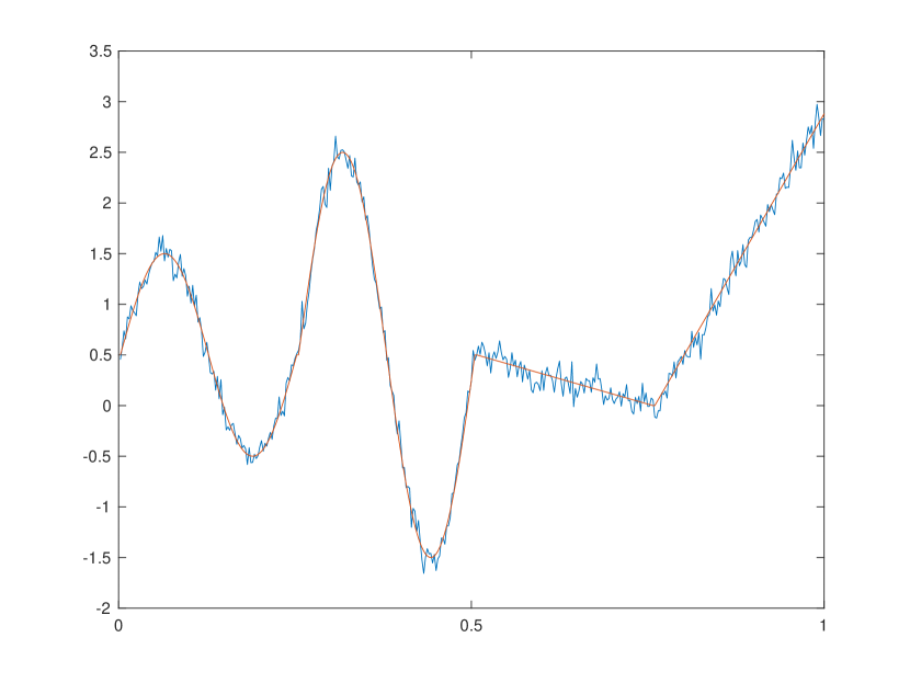
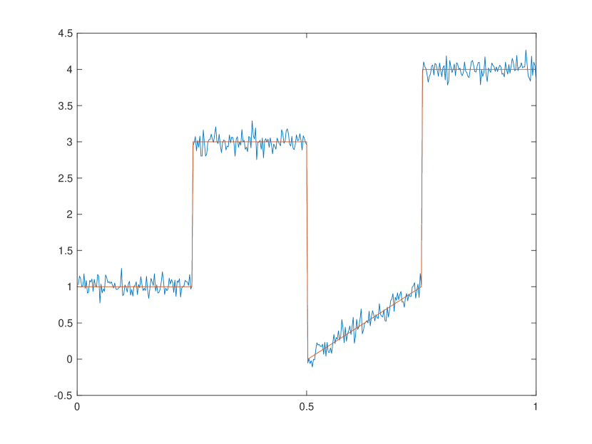
In order to gain further insight into the cost function $\mathcal{I}(\alpha,r)$, defined in (5.4), we compute it for a grid of values of $\alpha$ and $r$. We perform this analysis for two signals presenting different features, namely for a signal exhibiting corners (see Figure 1a) and for a signal with flat areas (see Figure 1b). In both cases, for simplicity, we assume $\alpha_{0}=\alpha_{1}=\alpha$ and we consider the discrete box-constraint

$$(\alpha,r)\in\left\{0,\,0.005,\,0.01,\,0.015,\ldots,2.5\right\}\times\left\{1,\,1.0025,\,1.005,\,\ldots,\,2\right\}$$ (6.1)

(see Remark 5.3). The reconstructed signal $u_{\alpha,r}$ in (5.3) is computed by using the primal-dual algorithm presented in [10] and [28].

a $u_{c}$ in red and $u_{\eta}=u_{c}+\eta$ in blue.

b $u_{c}$ in red and $u_{\eta}=u_{c}+\eta$ in blue.

Figure 1. The artificial noise $\eta$ is generated by using a Gaussian noise distribution.

The numerical landscapes of the cost function $\mathcal{I}(\alpha,r)$ are visualized in Figure 2a and Figure 2b, respectively.

a optimal $(\tilde{\alpha},\tilde{r})=(0.29,1.97)$

b optimal $(\tilde{\alpha},\tilde{r})=(0.05,1.35)$.

Figure 2. Numerical landscape (contour map) for the cost function $\mathcal{I}(\alpha,r)$. Darker colors correspond to smaller values of $\mathcal{I}(\alpha,r)$

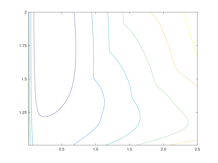
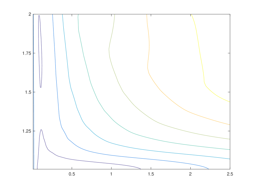
As we can see, in Figure 2b the optimal $\tilde{r}$ seems to lie away from the boundary of the discrete box-constraint (6.1), which are the integer values $r=1$ and $r=2$, showing an example in which the optimal signal reconstruction with respect to the $L^{2}$-distance can be achieved by the fractional order $TGV^{r}$. We can also see in Figure 3 that the optimal denoising results are quite satisfactory. However, it is also possible that the optimal result $\tilde{r}$ is an integer (in Figure 2a $\tilde{r}$ is indeed very close to an integer). For example, for a complete flat signal, i.e., $u_{c}\equiv 1$, then $u_{\alpha,1}=u_{c}$ for $\alpha$ large enough, provided that the noise $\eta$ satisfies $\int_{I}\eta(x)\,dx=0$ (zero-average assumption on noise is a reasonable assumption, see [42]). We point out once more that the introduction of fractional $r$-order $TGV^{r}$ only meant to expand the training choices for the bilevel scheme, but not to provide a superior seminorm to integer order $TGV^{k}$. The optimal solution $\tilde{r}\in[1,1/P]$, fractional order or integer order, is completely up to the given data $u_{c}$ and $u_{\eta}$.

Although from the numerical landscapes the cost function $\mathcal{I}(\alpha,r)$ (Figure 2) appears to be almost quasiconvex (see, [6, Section 3.4]) in the variable $\alpha$, this is not the case. In the forthcoming paper [21] some explicit counterexamples showing that at least for certain piecewise constant signals $\mathcal{I}\left(\alpha,1\right)$ is not quasiconvex will be presented. Additionally, Figure 2a and 2b both show that $\mathcal{I}(\alpha,r)$ is not quasiconvex in the $r$ variable. The non-quasiconvexity of the cost function $\mathcal{I}(\alpha,r)$, implies that the training scheme $(\mathcal{R})$ may not have a unique solution, i.e., the global minimizer of $\mathcal{I}(\alpha,r)$ might be not unique. In particular, the non-quasiconvexity of $\mathcal{I}(\alpha,r)$ prevents us from using standard gradient descent methods to find a global minimizer (which is the optimal solution we are looking for in (5.2)). Therefore, the identification of a reliable numerical scheme for solving the bilevel problem (upper level problem) remains an open question.

As a final remark, we point out that the development of a numerical scheme to identify the global minimizers of $\mathcal{I}(\alpha,1)$, $\alpha\in{\mathbb{R}}^{+}$ has been undertaken in [21], where the Bouligand differentiability and the finite discretization of $\mathcal{I}(\alpha,1)$ will be analyzed.

a The optimal denoised signal $u_{\tilde{\alpha},\tilde{r}}$ in blue

b The optimal denoised signal $u_{\tilde{\alpha},\tilde{r}}$ in blue

Figure 3. The optimal denoised signal $u_{\tilde{\alpha},\tilde{r}}$ in both cases are very close to the given clean signal.

References

- [1] R.A. Adams, J.J.F. Fournier. Sobolev spaces. Elsevier/Academic Press, Amsterdam, second edition, 2003.
- [2] L. Ambrosio, N. Fusco, D. Pallara. Functions of bounded variation and free discontinuity problems. Oxford Mathematical Monographs. The Clarendon Press, Oxford University Press, New York, 2000.
- [3] M. Bergounioux. Optimal control of problems governed by abstract elliptic variational inequalities with state constraints. SIAM J. Control Optim. 36(1) (1998), 273–289.
- [4] J. Bourgain, H. Brezis, P. Mironescu. Limiting embedding theorems for when and applications. J. Anal. Math. 87 (2002), 77–101.
- [5] J. Bourgain, H. Brezis, P. Mironescu. Another look at sobolev spaces. Optimal Control and Partial Differential Equations, J. L. Menaldi, E. Rofman, A. Sulem (Eds.), a volume in honor of A. Bensoussan’s 60th birthday, IOS Press, Amsterdam, pages 439–455, 2001.
- [6] S. Boyd, L. Vandenberghe. Convex optimization. Cambridge Univ. Press, Cambridge, 2004.
- [7] A. Braides. -convergence for beginners. Oxford Lecture Series in Mathematics and its Applications. Oxford University Press, Oxford, 2002.
- [8] K. Bredies, T. Valkonen. Inverse problems with second-order total generalized variation constraints. Proceedings of SampTA 2011 - 9th International Conference on Sampling Theory and Applications, Singapore, 2011.
- [9] M. Burger, K. Papafitsoros, E. Papoutsellis, C.-B. Schönlieb. Infimal convolution regularisation functionals of and spaces. Part I: the finite case. J. Math. Imaging Vision, 55(3) (2016), 343–369.
- [10] A. Chambolle, T. Pock. A first-order primal-dual algorithm for convex problems with applications to imaging. J. Math. Imaging Vision, 40 (1) (2011), 120–145.
- [11] T. Chan, A. Marquina, P. Mulet. High-order total variation-based image restoration. SIAM J. Sci. Comput. 22(2) (2000), 503–516.
- [12] D. Chen, S. Sun, C. Zhang, Y. Chen, D. Xue. Fractional-order - model for image denoising. Central European Journal of Physics, 11(10) (2013), 1414–1422.
- [13] Y. Chen, T. Pock, R. Ranftl, H. Bischof. Revisiting loss-specific training of filter-based mrfs for image restoration. In J. Weickert, M. Hein, and B. Schiele, editors, Pattern Recognition: 35th German Conference, GCPR 2013, Saarbrücken, Germany, September 3-6, 2013. Proceedings, pages 271–281. Springer Berlin Heidelberg, Berlin, Heidelberg, 2013.
- [14] Y. Chen, R. Ranftl, T. Pock. Insights into analysis operator learning: From patch-based sparse models to higher order mrfs. IEEE Transactions on Image Processing, 23(3) (2014), 1060–1072.
- [15] G. Dal Maso. An introduction to -convergence. Birkhäuser Boston, Inc., Boston, MA, 1993.
- [16] G. Dal Maso, I. Fonseca, G. Leoni, M. Morini. A higher order model for image restoration: the one-dimensional case. SIAM J. Math. Anal. 40(6) (2009), 2351–2391.
- [17] J. Dávila. On an open question about functions of bounded variation. Calc. Var. Partial Differential Equations, 15(4) (2002), 519–527.
- [18] E. Davoli, P. Liu. 2D Fractional order TGV: Gamma-convergence and bilevel training scheme. In preparation.
- [19] E. De Giorgi, T. Franzoni. Su un tipo di convergenza variazionale. Atti Accad. Naz. Lincei Rend. Cl. Sci. Fis. Mat. Natur. 58 (1975), 842–850.
- [20] J. C. De los Reyes, C.-B. Schönlieb. Image denoising: learning the noise model via nonsmooth PDE-constrained optimization. Inverse Probl. Imaging, 7(4) (2013), 1183–1214.
- [21] J. C. De los Reyes, P. Liu, C.-B. Schönlieb. Numerical analysis of bilevel parameter training scheme in total variation image reconstruction. In preparation.
- [22] J. C. De los Reyes, C.-B. Schönlieb, T. Valkonen. Bilevel parameter learning for higher-order total variation regularisation models. J. Math. Imaging Vision, (2016), 1–25.
- [23] M. Benning, C.-B. Schönlieb, T. Valkonen. Vlačić, V. Explorations on anisotropic regularisation of dynamic inverse problems by bilevel optimisation. ArXiv:1602.01278, (2017).
- [24] J.C. De los Reyes, C.-B. Schönlieb, T. Valkonen. The structure of optimal parameters for image restoration problems. J. Math. Anal. Appl. 434(1) (2016), 464–500.
- [25] E. Di Nezza, G. Palatucci, E. Valdinoci. Hitchhiker’s guide to the fractional Sobolev spaces. Bull. Sci. Math. 136(5) (2012), 521–573.
- [26] J. Domke. Generic methods for optimization-based modeling. In N.D. Lawrence and M.A. Girolami, editors, Proceedings of the Fifteenth International Conference on Artificial Intelligence and Statistics (AISTATS-12), volume 22, pages 318–326, 2012.
- [27] J. Domke. Learning graphical model parameters with approximate marginal inference. IEEE Transactions on Pattern Analysis and Machine Intelligence, 35(10) (2013), 2454–2467.
- [28] J.B. Garnett, T.M. Le, Y. Meyer, L.A. Vese. Image decompositions using bounded variation and generalized homogeneous Besov spaces. Appl. Comput. Harmon. Anal. 23(1) (2007), 25–56.
- [29] N.S. Landkof. Foundations of modern potential theory. Springer-Verlag, New York-Heidelberg, 1972.
- [30] G. Leoni. A first course in Sobolev spaces. American Mathematical Society, Providence, RI, 2009.
- [31] V.G. Maz\cprimeya, T.O. Shaposhnikova. On the Bourgain, Brezis, and Mironescu theorem concerning limiting embeddings of fractional Sobolev spaces. J. Funct. Anal. 195(2) (2002), 230–238.
- [32] V.G. Maz\cprimeya, T.O. Shaposhnikova. Theory of Sobolev multipliers. Springer-Verlag, Berlin, 2009.
- [33] K. Papafitsoros, K.Bredies. A study of the one dimensional total generalised variation regularisation problem. Inverse Probl. Imaging, 9(2) (2015), 511–550.
- [34] K. Papafitsoros, C.B. Schönlieb. A combined first and second order variational approach for image reconstruction. J. Math. Imaging Vision, 48(2) (2014), 308–338.
- [35] L.I. Rudin. Segmentation and restoration using local constraints. Cognitech Report 36 (1993).
- [36] L.I. Rudin, S. Osher. Total variation based image restoration with free local constraints. In Image Processing, 1994. Proceedings. ICIP-94., IEEE International Conference, volume 1, pages 31–35 vol.1, Nov 1994.
- [37] L.I. Rudin, S. Osher, E. Fatemi. Nonlinear total variation based noise removal algorithms. Phys. D, 60 (1992), 259–268.
- [38] J. Simon. Sobolev, Besov and Nikol\cprimeskiĭ fractional spaces: embeddings and comparisons for vector valued spaces on an interval. Ann. Mat. Pura Appl. 157 (1990), 117–148 .
- [39] M.F. Tappen. Utilizing variational optimization to learn markov random fields. In 2007 IEEE Conference on Computer Vision and Pattern Recognition, pages 1–8, June 2007.
- [40] M.F. Tappen, C. Liu, E.H. Adelson, W.T. Freeman. Learning gaussian conditional random fields for low-level vision. In 2007 IEEE Conference on Computer Vision and Pattern Recognition, pages 1–8, June 2007.
- [41] H. Triebel. Theory of function spaces. Modern Birkhäuser Classics. Birkhäuser/Springer Basel AG, Basel, 2010.
- [42] Chambolle, Antonin and Lions, Pierre-Louis. Image recovery via total variation minimization and related problems. Numer. Math., 1997
- [43] T. Valkonen, K. Bredies, F. Knoll. Total generalized variation in diffusion tensor imaging. SIAM J. Imaging Sci. 6(1) (2013), 487–525.