Correlated stopping, proton clusters and higher order proton cumulants

Abstract

We investigate possible effects of correlations between stopped nucleons on higher order proton cumulants at low energy heavy-ion collisions. We find that fluctuations of the number of wounded nucleons $N_{\mathrm{part}}$ lead to rather nontrivial dependence of the correlations on the centrality; however, this effect is too small to explain the large and positive four-proton correlations found in the preliminary data collected by the STAR collaboration at $\sqrt{s}=7.7$ GeV. We further demonstrate that, by taking into account additional proton clustering, we are able to qualitatively reproduce the preliminary experimental data. We speculate that this clustering may originate either from collective/multi-collision stopping which is expected to be effective at lower energies or from a possible first-order phase transition, or from (attractive) final state interactions. To test these ideas we propose to measure a mixed multi-particle correlation between stopped protons and a produced particle (e.g. pion, antiproton).

I Introduction

The structure of the phase diagram is one of the fundamental problems of the theory of strong interactions, quantum chromodynamics (QCD); a variety of solutions to this problems are pursued in both theoretical and experimental studies. From the theory side, the thermodynamics of QCD is explored by the number of approaches including first principle numerical lattice QCD (LQCD) Borsanyi et al. (2010); Endrodi et al. (2011); Bazavov et al. (2012); Borsanyi et al. (2012); Bellwied et al. (2013); Borsanyi et al. (2014a); Bhattacharya et al. (2014); Borsanyi et al. (2014b); Bazavov et al. (2014); Ding et al. (2015); Bellwied et al. (2015); Aarts (2016); Ratti (2016), functional methods Fischer et al. (2014); Herbst et al. (2014); Mitter et al. (2015); Chatterjee and Mohan (2015) and effective models of QCD Fukushima (2004); Roder et al. (2003); Skokov et al. (2011); Friman et al. (2011); Pisarski and Skokov (2016). Experimental studies of the hot and dense matter created in heavy-ion collisions are also ongoing Adamczyk et al. (2014) or planned to be carried out in the near future Chattopadhyay et al. (2016).

The LQCD results show that, at the physical pion mass, hot nuclear matter exhibits residual properties of both dynamical chiral symmetry breaking and confinement at finite temperature. In the LQCD calculations, it was demonstrated that the transition between hadrons and quark/gluon degrees of freedom is of crossover type Aoki et al. (2006). At finite baryon densities, progress of LQCD calculations is impeded by the notorious sign problem. Several attempts to circumvent the sign problem were carried out Fodor and Katz (2002); D’Elia and Lombardo (2003); Allton et al. (2002); Fodor and Katz (2004); Bonati et al. (2014); de Forcrand and Philipsen (2010). Some of these studies indicate the existence of the expected critical point (CP) at a finite value of the baryon chemical potential Fodor and Katz (2002, 2004).

In experiment, the fluctuations of the conserved charges are believed to be a promising probe of the QCD critical point. Based on universality arguments, it was predicted that the higher order cumulants of baryon/charge number fluctuations are very sensitive to the correlation length, $\xi$, and thus convey the information about the underlying behaviour of the critical mode Stephanov et al. (1999); Ejiri et al. (2006); Stephanov (2009, 2011). Quantitatively, it was shown that the singular parts of the cumulants of the net baryon/charge distribution scale with the correlation length according to $\chi^{\rm sing}_{n}\propto\xi^{\frac{n\beta\delta}{\nu}-3}$ where $\beta$, $\delta$ and $\nu$ are critical exponents of the three-dimensional Ising universality class. However, this sensitivity of the higher order cumulants to the critical dynamics does not come for free: they probe the tails of the probability distribution which are also susceptible to various non-critical effects including baryon number conservation Bzdak et al. (2013), volume or number of wounded nucleon fluctuations Skokov et al. (2013); Xu (2016); Braun-Munzinger et al. (2016), detector efficiency and acceptance Bzdak and Koch (2015); Ling and Stephanov (2016); Bzdak et al. (2016a); Luo (2015a); Kitazawa (2016); Nonaka et al. (2016), hadronic rescattering Kitazawa and Asakawa (2012a), deuteron formation Fecková et al. (2015), non-equilibrium effects Mukherjee et al. (2015, 2016), non-critical correlations between centrality trigger and the observable, etc.

Recent experimental results collected in the Beam Energy Scan, a dedicated experimental program at RHIC, demonstrated a non-monotonic dependence of the fourth order cumulant or kurtosis of net proton fluctuations on the energy of collisions Adamczyk et al. (2014). Experiments also showed, that, at low energies or, equivalently, higher baryon densities, the kurtosis increases with decreasing collision energy. In the central rapidity region, where most of the measurements are performed, the baryon stopping is what makes the high baryon densities possible. Indeed at low energies, where proton-antiproton pair-production is negligible, all the observed protons originate from the target and projectile. Therefore, the dynamics of baryon stopping is yet another source of fluctuations which can distort the measurement and can be potentially responsible for the non-monotonic behavior of the kurtosis Bialas et al. (2016).

An analysis of the genuine multi-particle correlations Bzdak et al. (2016b) found that these correlations have a range of the order or larger than one unit of rapidity, $\delta y\geq 1$. Typically, long-range correlations in rapidity suggest the correlations to be formed early in the evolution of the fireball, although this argument is less stringent at the lower energies. Therefore, it would be worthwhile to study the effect of initial conditions, such as so-called volume or rather participant fluctuations as well as effects of stopping.

It is the purpose of this paper to address some of these issues. We will explore the influence of wounded nucleon Bialas et al. (1976) fluctuations as well as fluctuations due to multi-collision nucleon stopping, effectively resulting in proton clusters, on the correlation functions at low energies. We show that for the integrated $n$-particle correlation functions, $C_{n}$, the effect of wounded nucleon fluctuations is small for $n>2$ and negligible for $C_{4}$. However, for $C_{2}$, we find that this contribution is quite significant. Additionally, we show that taking into account multi-proton clusters reproduces the right order of magnitude of the experimental values for $C_{n}$.

This manuscript is organized as follows: In Sec. II, we briefly review the definition of the correlation functions previously discussed in Ref. Bzdak et al. (2016b). In Sec. III, we explore the effect of the wounded nucleon fluctuations. Additional sources of correlations due to proton clustering is discussed in Sec. IV. We conclude with Sec. V.

II Notation

Let us start by defining our notation. The proton multiplicity distribution measured in a given rapidity bin, $\Delta y$, will be denoted by $P(N)$. The corresponding generating function $H(z)$ is given by

$$H(z)=\sum\nolimits_{N}P(N)z^{N},\qquad H(1)=1;$$ (1)

so that the factorial moments $F_{k}$ of the proton multiplicity distribution can be obtained by taking the appropriate number of derivatives of $H(z)$:

$$F_{k}\equiv\left\langle N(N-1)\cdots(N-k+1)\right\rangle=\left.\frac{d^{k}}{dz^{k}}H(z)\right|_{z=1}.$$ (2)

We note that the first factorial moment corresponds to the average number of particles, $F_{1}=\langle N\rangle$, the second factorial moment $F_{2}=\langle N(N-1)\rangle$ gives the number of pairs, $F_{3}$ the number of triplets etc. The integrated $k$-particle correlation function $C_{k}$, also known as the factorial cumulant $\kappa_{k}$ Ling and Stephanov (2016), is given by

$$C_{k}=\left.\frac{d^{k}}{dz^{k}}C(z)\right|_{z=1},\qquad C(z)=\ln\left[H(z)\right],$$ (3)

with $C_{1}=\left\langle N\right\rangle$. As an example, consider the two-particle rapidity correlation function

$$C_{2} = \left\langle N(N-1)\right\rangle-\left\langle N\right\rangle^{2}$$ (4)

$$= \int_{\Delta y}dy_{1}dy_{2}\left[\rho_{2}(y_{1,}y_{2})-\rho_{1}(y_{1})\rho_{1}(y_{2})\right]$$

$$= \int_{\Delta y}dy_{1}dy_{2}C_{2}(y_{1},y_{2});$$

this can be indeed recognized as the proper definition of the integrated two-particle correlation function. Here $C_{2}(y_{1},y_{2})$ is the differential correlation function in rapidity, and $\rho_{2}(y_{1,}y_{2})$ and $\rho_{1}(y)$ are the two-particle and the single-particle rapidity distributions, respectively.

It is convenient to define the reduced correlation functions $c_{k}$ which, following Ref. Bzdak et al. (2016b), we shall refer to as couplings

$$c_{k}=\frac{C_{k}}{\left\langle N\right\rangle^{k}}.$$ (5)

Finally, the proton cumulants, $K_{n}$, as recently measured by the STAR Collaboration, are related to the integrated correlation functions $C_{n}$ through

$$K_{1} \equiv \langle N\rangle=C_{1},$$

$$K_{2} \equiv \langle(\delta N)^{2}\rangle=\left\langle N\right\rangle+C_{2},$$

$$K_{3} \equiv \langle\left(\delta N\right)^{3}\rangle=\left\langle N\right\rangle+3C_{2}+C_{3},$$

$$K_{4} \equiv \langle\left(\delta N\right)^{4}\rangle-3\langle(\delta N)^{2}\rangle^{2}=\left\langle N\right\rangle+7C_{2}+6C_{3}+C_{4},$$ (6)

where $\delta N=N-\langle N\rangle$. As was recently emphasized in Refs. Ling and Stephanov (2016); Bzdak et al. (2016b), the cumulants mix the correlation functions of different orders.

In Ref. Bzdak et al. (2016b), the correlation functions $C_{n}$ and the couplings $c_{n}$ were extracted from the preliminary STAR data Luo (2015b, 2016). Here we highlight the most important conclusions from this analysis. For peripheral collisions at $\sqrt{s}=7.7$ GeV, the couplings $c_{k}$ scale like $1/N^{k-1}$; this is consistent with the production from independent sources. At $N_{\text{part}}\sim 200,$ the correlations $C_{3}$ and $C_{4}$ change signs and reach large values for the most central collisions

$$6C_{3}\sim-60,\quad 6c_{3}\sim-10^{-3}\,;\quad\quad C_{4}\sim 170,\quad c_{4}\sim 10^{-4},$$ (7)

both with large error bars. $C_{3}$ and $C_{4}$ decrease with the increasing energy and at $\sqrt{s}=19.6$ GeV they are consistent with zero for $N_{\text{part}}\approx 350$ whereas $C_{2}$ does not vary significantly and approximately equals $7C_{2}\sim-15$ at all energies. After these preliminaries let us now discuss the effect of volume or rather participant fluctuations on the correlation functions.

III Correlations from fluctuations of the number of wounded nucleons

Fluctuations of the number of wounded or participating nucleons $N_{\text{part}}$, which in the context of fluctuation studies are often referred to as volume fluctuation Koch et al. (2001); Koch (2010); Skokov et al. (2013), constitute one of the more obvious sources for correlations and fluctuations of the final protons. Also, at low energies, where baryon pair-production is negligible, practically all observed protons at mid-rapidity originate from stopped target and projectile nucleons. Since pions are abundant even at $7.7{\rm\,GeV}$, isospin exchange reactions should be very fast and, thus, the observed protons may originate equally likely from stopped protons and neutrons Kitazawa and Asakawa (2012a, b). This allows us to formulate the following minimal model which takes into account fluctuations of the number of wounded nucleons, baryon number conservation Bzdak et al. (2013) and fast isospin exchange: Based on the Glauber model (see, e.g., Ref. Alver et al. (2008)), a certain centrality selection determines the distribution of participating nucleons $P\left(N_{\text{part}}\right)$. Given the number of participating nucleons $N_{\text{part}}$ in an event, the number of protons $N$ observed in $\Delta y$ then follow a binomial distribution $B(N;N_{\text{part}};p)$, where $p=\left\langle N\right\rangle/\left\langle N_{\text{part}}\right\rangle$ is the probability for any wounded nucleon to end up in the rapidity interval $\Delta y$ as a proton. Here, $\left\langle N\right\rangle$ is the observed mean number of protons in the rapidity interval $\Delta y$, and $\left\langle N_{\text{part}}\right\rangle$ is the average number of wounded nucleons for a given centrality selection. Obviously this model assumes that each nucleon stops independently from the other; this finds some support at higher energies Basile et al. (1983). Thus, the probability $P(N)$ to observe $N$ protons in $\Delta y$ is given by

$$P(N)=\sum\nolimits_{N_{\text{part}}}P(N_{\text{part}})\frac{N_{\text{part}}!}{N!(N_{\text{part}}-N)!}p^{N}(1-p)^{N_{\text{part}}-N},$$ (8)

and

$$H(z)=\sum\nolimits_{N_{\text{part}}}P(N_{\text{part}})\left[1-p+pz\right]^{N_{\text{part}}}.$$ (9)

Given the above generating function, the correlation functions $C_{k}$ and couplings $c_{k}$ as defined in Sec. II can be computed (see also the Appendix):

$$c_{2} = -\frac{1}{\left\langle N_{\text{part}}\right\rangle}+\frac{\langle\left[N_{\text{part}}-\left\langle N_{\text{part}}\right\rangle\right]^{2}\rangle}{\left\langle N_{\text{part}}\right\rangle^{2}},$$ (10)

$$c_{3} = \frac{2}{\left\langle N_{\text{part}}\right\rangle^{2}}+\frac{\langle\left[N_{\text{part}}-\left\langle N_{\text{part}}\right\rangle\right]^{3}\rangle-3\langle\left[N_{\text{part}}-\left\langle N_{\text{part}}\right\rangle\right]^{2}\rangle}{\left\langle N_{\text{part}}\right\rangle^{3}},$$ (11)

$$c_{4} = -\frac{6}{\left\langle N_{\text{part}}\right\rangle^{3}}+$$ (12)

$$\frac{\langle\left[N_{\text{part}}-\left\langle N_{\text{part}}\right\rangle\right]^{4}\rangle-3\langle\left[N_{\text{part}}-\left\langle N_{\text{part}}\right\rangle\right]^{2}\rangle^{2}+11\langle\left[N_{\text{part}}-\left\langle N_{\text{part}}\right\rangle\right]^{2}\rangle-6\langle\left[N_{\text{part}}-\left\langle N_{\text{part}}\right\rangle\right]^{3}\rangle}{\left\langle N_{\text{part}}\right\rangle^{4}},$$

where

$$\left\langle N_{\text{part}}^{n}\right\rangle=\sum\nolimits_{N_{\text{part}}}P(N_{\text{part}})N_{\text{part}}^{n}\text{.}$$ (13)

In absence of fluctuations in the number of participants, that is $P(N_{\text{part}})=\delta_{N_{\text{part}},\left\langle N_{{\text{part}}}\right\rangle}$ in Eq. (8), the couplings, $c_{k}$, reduce to

$$c_{2}\to-\frac{1}{\left\langle N_{\text{part}}\right\rangle},\quad c_{3}\to\frac{2}{\left\langle N_{\text{part}}\right\rangle^{2}},\quad c_{4}\to-\frac{6}{\left\langle N_{\text{part}}\right\rangle^{3}}.$$ (14)

In this case, the couplings, $c_{n}$, as functions of the order, $n$, alternate in sign and are suppressed by powers of the mean number of participants, $\sim 1/\left\langle N_{\text{part}}\right\rangle^{n-1}$. This behavior is qualitatively consistent with the analysis of the preliminary STAR data for peripheral collisions, $N_{\text{part}}<200$ Bzdak et al. (2016b). As expected, the couplings, Eqs. (10-12), do not depend on the binomial probability $p=\left\langle N\right\rangle/\left\langle N_{\text{part}}\right\rangle$, because (binomial) efficiency corrections do not alter the reduced correlations functions (see e.g. Ref. Pruneau et al. (2002)).

III.1 Monte Carlo calculation

To calculate the contribution of $N_{\text{part}}$ fluctuations to the multi-particle correlations $C_{k}$ and the couplings $c_{k}$ we need to define the centrality of the collision. Following the STAR procedure, see e.g. Ref. Luo (2015b), we use the tightest centrality cuts, that is, we calculate $c_{k}$ and $C_{k}$ at a given number of produced charged particles (except protons) $N_{\text{ch}}$ in $|\eta|<1$ Luo (2015b).

In our analysis we first calculate $N_{\text{part}}$ using a standard Glauber model, see, e.g. Ref. Alver et al. (2008). We used $\sigma_{\text{in}}=31$ mb for $\sqrt{s}=7.7$ GeV. Next, for each $N_{\text{part}}$ we sampled charged particles from the Poisson distribution with the average $\langle N_{\text{ch}}\rangle$ in $|\eta|<1$ given by

$$\left\langle N_{\text{ch}}\right\rangle|_{N_{\text{part}}}=aN_{\text{part}}\left(N_{\text{part}}/2\right)^{0.1}.$$ (15)

Here we take $a=0.75$ for $\sqrt{s}=7.7$ GeV. We verified that small variations in the value of $a$ do not change our conclusions (see Sec. V for further discussion). Let us comment on $\left(N_{\text{part}}/2\right)^{0.1}$. It is well known that in the midrapidity region, the number of charged particles grows a bit faster than $N_{\text{part}}$, see e.g. Refs. Adcox et al. (2001); Back et al. (2006). For example, in Au+Au collisions at RHIC energies, $\left\langle N_{\text{ch}}\right\rangle/N_{\text{part}}$ grows roughly by a factor of $1.7$ between proton-proton ($N_{\text{part}}=2$) and central Au+Au collisions ($N_{\text{part}}\simeq 350$). This feature can be easily understood in the wounded constituent quark (quark-diquark) model Eremin and Voloshin (2003); Bialas and Bzdak (2007), where nucleons undergoing several collisions generate more particles than protons in p+p collisions.

After generating a sufficient number of events, for each value of $N_{\text{ch}}$ we calculate $\left\langle N_{\text{part}}\right\rangle,$ $\left\langle N_{\text{part}}^{2}\right\rangle$ etc. and evaluate the couplings $c_{k}$ following Eqs. (10-12). Our results for $c_{2}$, $c_{3}$, and $c_{4}$ are shown in Fig. 1 by the solid (red) curves. The (blue) dashed curves represent the results without volume ($N_{\text{part}}$) fluctuations (no VF), see Eq. (14).

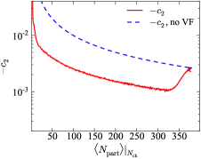
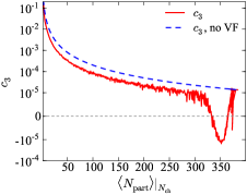
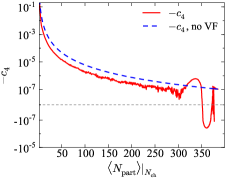
Figure 1: The couplings $-c_{2},c_{3},-c_{4}$ for $\sqrt{s}=7.7$ GeV in Au+Au collisions as a function of $\langle N_{\text{part}}\rangle|_{N_{\text{ch}}}$ at a given number of charged particles $N_{\text{ch}}$. The (blue) dashed curves represent the results without fluctuations of the number of wounded nucleons (“no VF”), see Eq. (14).

We observe that $N_{\mathrm{part}}$ fluctuations lead to rather nontrivial effects in very central collisions. The coupling $-c_{2}$ changes the trend from decreasing to increasing with growing $N_{\text{ch}}$ (mind the minus sign in front of $c_{2}$ plotted in in Fig. 1), and both $c_{3}$ and $c_{4}$ change signs. Interestingly, similar trends were observed for $c_{k}$ extracted from the preliminary STAR data, see Ref. Bzdak et al. (2016b), although the effects for $c_{3}$ and $c_{4}$ observed in Fig. 1 are at least an order of magnitude too small for $c_{3}$, and roughly three orders of magnitude too small for $c_{4}$, see Eq. (7). Moreover, in our results the signs change only for very central collisions whereas in the analysis of the preliminary data this change is present at about $N_{\text{part}}\sim 200$. Finally, as we shall discuss below, the sharp wiggles observed in $c_{3}$ and $c_{4}$ disappear once one averages the couplings over a centrality region of $5\%$, as it is done in the STAR analysis Luo (2015b).

In order to illustrate the contribution from $N_{\text{part}}$ fluctuations let us factor out the leading term $c_{k}\sim 1/\left\langle N_{\text{part}}\right\rangle^{k-1}$ from $c_{2}$, $c_{3}$ and $c_{4}$ in Eqs. (10-12), that is define $R_{n}$ according to

$$-\frac{1}{\left\langle N_{\text{part}}\right\rangle}\left(1-R_{2}\right) \overset{\mathrm{def}}{=} c_{2},$$ (16)

$$\frac{2}{\left\langle N_{\text{part}}\right\rangle^{2}}\left(1-R_{3}\right) \overset{\mathrm{def}}{=} c_{3},$$ (17)

$$-\frac{6}{\left\langle N_{\text{part}}\right\rangle^{3}}\left(1-R_{4}\right) \overset{\mathrm{def}}{=} c_{4},$$ (18)

so that $R_{2}$, $R_{3}$ and $R_{4}$ represent the ratios of the contributions from $N_{\text{part}}$ fluctuations over those arising without $N_{\text{part}}$ fluctuations in Eq. (14). In Fig. 2 we plot these ratios as functions of $\left\langle N_{\text{part}}\right\rangle|_{N_{\text{ch}}}$.

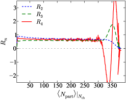
Figure 2: Relative contribution of $N_{\text{part}}$ fluctuation, see Eqs. (16,17,18), for $c_{2},c_{3}$ and $c_{4}$ at $\sqrt{s}=7.7$ GeV in Au+Au collisions.

Even though we apply the tightest centrality cuts, (we fix the number of charged particles with the finest possible bin width) we find corrections of $50\%$ or more for off-central collisions and much larger modification in the most central collisions.

Finally, let us calculate the integrated correlation functions $C_{k}=\left\langle N\right\rangle^{k}c_{k}$; they are directly related to the cumulants measured by STAR, see Eq. (6). To proceed we need to determine the dependence of the average number of protons, $\left\langle N\right\rangle$, on $N_{\text{part}}$. From the preliminary STAR data Luo (2015b) we get

$$\left\langle N\right\rangle|_{N_{\text{ch}}}=b\left(\frac{\left\langle N_{\text{part}}\right\rangle|_{N_{\text{ch}}}}{337}\right)^{1.25},$$ (19)

where $b=40$ for $\sqrt{s}=7.7$ GeV. Our conclusions are not sensitive to small variations of $b$ and changing the exponent from $1.25$ to $1$. The results are presented in Fig. 3 by the solid curves. The dashed curves correspond to calculations without volume ($N_{\text{part}}$) fluctuations (no VF). The symbols represent the correlations after averaging over bins in centrality of $5\%$, i.e. $0-5\%$, $5-10\%$ etc. Only the five most central points are shown. For less central collisions, the centrality averaging does not alter our results and points fall right on the solid lines. Clearly, the contribution originating from $N_{\text{part}}$ fluctuations is important for the two particle correlation, $C_{2}$; there is also some but less significant effect of $N_{\text{part}}$ fluctuations on the three particle correlation $C_{3}$ in central collisions. On the other hand, when compared to the STAR data, fluctuations of wounded nucleons are all but irrelevant for the four particle correlation, $C_{4}$. In our model calculation, $C_{4}$ is negative for off-central collisions and it gets positive for large $N_{\text{part}}$. After averaging over centrality bins, the model predicts around $-0.3$ for $C_{4}$ while the analysis of the preliminary STAR data gives $\sim 170$. Also, as already mentioned, the strong oscillations exhibited in $C_{3}$ and $C_{4}$ at large $N_{\text{part}}$ disappear after averaging over centrality bins. Obviously our model of independent stopping together with baryon number conservation clearly fails to explain the preliminary STAR data, reported in Ref. Bzdak et al. (2016b) (see Fig. 1 therein).

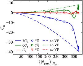
Figure 3: Multi-particle correlations $C_{n}$ in Au+Au collisions at $\sqrt{s}=7.7$ GeV. The leading terms, where fluctuations of the number of wounded nucleons are not present, are denoted by “no VF”. Also shown as circles, triangles and squares are the results for the five most central bins with a width of $5\%$ of centrality.

Before we close this section, let us make a few more remarks. First, the results without the number of wounded nucleon fluctuations presented in this section can be verified analytically. At a fixed $N_{\text{part}}$, Eq. (9) reduces to

$$H(z;N_{\text{part}})=(1-p+pz)^{N_{\text{part}}},$$ (20)

and using Eq. (3) we obtain

$$C_{2}=-p^{2}N_{\text{part}},\text{\quad}C_{3}=2p^{3}N_{\text{part}},\quad C_{4}=-6p^{4}N_{\text{part}}\text{.}$$ (21)

Since $p<1$ this explains the relative magnitude of the correlation functions. Next, in our analysis we assumed that each nucleon is stopped in $\Delta y$ with the same probability $p$. This is rather unphysical since nucleons that collide once are expected to have significantly smaller $p$ than nucleon from the centers which collide several times. However, as long as we have independent stopping of the nucleons, individual stopping probabilities do not really change our conclusions. Suppose that each nucleon is characterized by its own stopping probability, $p_{(i)}$, $i=1,...,N_{\text{part}}$. Neglecting $N_{\text{part}}$ fluctuations we obtain at a given $N_{\text{part}}$

$$H(z;N_{\text{part}})=\prod\nolimits_{i=1}^{N_{\text{part}}}(1-p_{(i)}+p_{(i)}z),$$ (22)

which obviously reduces to Eq. (20) if $p_{i}=p$. Calculating $C_{k}$ we observe that it is enough to replace $N_{\text{part}}p^{n}\rightarrow\sum\nolimits_{i}p_{(i)}^{n}$ in Eq. (21) and thus the signs of $C_{k}$ do not change. We conclude that this effect cannot lead to a large and positive $C_{4}$ as seen in the STAR data.

The corollary of this section is the following. The two-particle correlations obtained in our model of independent nucleon stopping together with baryon-number conservation and fast isospin equilibration are of the same magnitude as in the preliminary STAR data. Also, the model produces a non-negligible three-particle correlation. On the other hand, the model four-particle correlation comes out to be almost three orders of magnitude smaller than in the preliminary STAR data at $\sqrt{s}=7.7$ GeV.  The large discrepancy of the four-particle correlation between our model and the preliminary data suggests that additional strong effects must be at play. In the following section, we will explore what happens if we relax the assumption of independent stopping of nucleons and allow for proton clustering.

IV Proton clusters

In this section go we go beyond the independent stopping assumption and consider a possible clustering of protons. This clustering can be attributed to, e.g., the collective stopping or to a first order phase transition. We note, that little is known about the stopping of nucleons at lower energies, and, therefore, this discussion is somewhat speculative and should be considered merely as a motivation to explore the stopping mechanism in more detail.

In our view, it is not at all obvious that the standard Glauber model still provides the correct stopping framework at energies as low as $\sqrt{s}=7.7$ GeV. Indeed, it seems plausible that a nucleon passing through a center of a nuclei may actually loose enough energy and start undergoing elastic scatterings leading to an inter-nucleus cascade. This may lead to some multi-particle correlations between stopped protons. For example, in the extreme case when two protons scatter elastically they go back-to-back and they either both end up in our rapidity bin or they both go outside. This obviously results in two-particle rapidity correlations since protons tend to come in pairs. In central collisions more protons can be involved in this multi-collision (quasi-) elastic stopping, and thus, higher-order proton multiplets are not a priori excluded. We note that this mechanism is expected to turn on at relatively low collision energy and in central collisions, where protons collide several times, and thus may lose sufficient energy to engage in subsequent elastic scatterings. In other words, the stopped protons from the centers effectively form proton clusters. Of course cluster formation may also arise from a first order phase transition (see, e.g., Skokov and Voskresensky (2009a, b); Steinheimer and Randrup (2012)) or final state interactions and it will require more detailed study to disentangle the various possibilities.

We explored various scenarios where protons come in pairs, triplets and higher-order multiplets. We found that it is not an easy task to reproduce $C_{2}<0$, $C_{3}<0$ and $C_{4}>0$ with $6C_{3}$ and $C_{4}$ of the order of $100$ for $\sqrt{s}=7.7$ GeV, as seen in Ref. Bzdak et al. (2016b). To discuss this in more detail, let us focus on central $\sqrt{s}=7.7$ GeV collisions, were the signal is strongest. In this case $\left\langle N\right\rangle\simeq 40$, $7C_{2}\simeq-15$, $6C_{3}\simeq-60$, and $C_{4}\simeq 170$. Before we discuss two scenarios which give results in the right ballpark, let us put the difficulty of the task in perspective. Consider a system of clusters distributed according to a Poisson distribution which decay into a fixed number of protons, $m$. In this case, the generating function is given by

$$H_{\text{Poisson}}(z)=\exp\left[\left\langle N_{\rm cl}\right\rangle\left(z^{m}-1\right)\right],$$ (23)

where $\left\langle N_{\rm cl}\right\rangle$ is the average number of clusters. The resulting integrated correlation functions $C_{k}$ are given by $C_{k}=\left\langle N_{\rm cl}\right\rangle m!/(m-k)!$ so that for four-particle clusters ($m=4$) we have $C_{4}=24\left\langle N_{\rm cl}\right\rangle$. Thus, in order to get $C_{4}\simeq 170$ we need on average $6-8$ clusters, about 25 of the 40 observed protons would have to originate from clusters, a rather large fraction indeed. Of course the same cluster model would also lead to positive two- and three-particle correlations, contrary to what is seen in the data.

Let us now turn to discuss two scenarios which lead to a correlation structure in qualitative agreement with the preliminary STAR data. Consider central Au+Au collisions and suppose that nucleons at the surface (and in general those who do not scatter sufficiently often) are stopped according to a simple string picture, and, thus, follow the previously discussed model of independent binomial stopping. Next, suppose that nucleons from the centers of target and projectile, which scatter several times, loose most of the energy and engage in elastic scattering and, thus, fall into $\Delta y$ in pairs. In this case the generating function is given by

$$H(z;N_{\text{part}})=\left(1-p_{1}+p_{1}z\right)^{N_{\text{part}}-2M}\left(1-p_{2}+p_{2}z^{2}\right)^{M},$$ (24)

where $M$ is the number of pairs. Let us clarify the above formula. $N_{\text{part}}-2M$ nucleons either stop in $\Delta y$ with the probability $p_{1}$ or they do not with the probability $1-p_{1}$, and the generating function for each nucleon is simply given by $(1-p_{1})z^{0}+p_{1}z^{1}$. In the second term we have $M$ pairs which either fall into $\Delta y$ with probability $p_{2}$ or they do not with the probability $1-p_{2}$. In this case we either get $0$ or $2$ protons (from each pair) and the pair generating function is given by $(1-p_{2})z^{0}+p_{2}z^{2}$. We also expect that $p_{2}$ is much larger than $p_{1}$ since pairs loose energy due to scatterings and are likely to fall into the midrapidity bin of interest $\Delta y$ (for STAR $\Delta y\in[-0.5,0.5]$).

The multi-particle correlations $C_{k}$ are given by the appropriate derivatives (at $z=1$) of

$$C(z;N_{\text{part}}) = \ln\left[H(z;N_{\text{part}})\right]$$ (25)

$$= (N_{\text{part}}-2M)\ln\left(1-p_{1}+p_{1}z\right)+M\ln\left(1-p_{2}+p_{2}z^{2}\right)$$

resulting in

$$\left\langle N\right\rangle = p_{1}\left(N_{\text{part}}-2M\right)+2p_{2}M,$$

$$C_{2} = -p_{1}^{2}\left(N_{\text{part}}-2M\right)-2p_{2}\left(2p_{2}-1\right)M,$$

$$C_{3} = 2p_{1}^{3}\left(N_{\text{part}}-2M\right)-4p_{2}^{2}\left(3-4p_{2}\right)M,$$

$$C_{4} = -6p_{1}^{4}\left(N_{\text{part}}-2M\right)+12p_{2}^{2}\left(8p_{2}-8p_{2}^{2}-1\right)M.$$ (26)

Taking $N_{\text{part}}=350$, $\left\langle N\right\rangle=0.12N_{\text{part}}=42$ and $M=8$ ($8$ pairs of protons) we obtain the relation between $p_{1}$ and $p_{2}$. In Fig. 4 (left) we plot $7C_{2},$ $6C_{3}$ and $C_{4}$ as a function of $p_{2}$. We observe that for $p_{2}>0.5$ both $C_{3}$ and $C_{4}$ have the right signs and can reach substantial values.

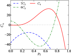
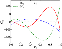
Figure 4: Integrated multi-particle correlations $C_{n}$ in the model where particles are correlated in pairs (left) and quartets (right) as a function of the probability for a pair ($p_{2}$) or a quartet ($p_{4}$) to end up in the rapidity bin. For larger values of $p_{2}$ and $p_{4}$ we obtain large values of $C_{3}$ and $C_{4}$. See the text for further explanation.

The right panel of Fig. 4 shows the results of an analogues calculation where protons come in quartets instead of pairs. In this case

$$C(z;N_{\text{part}})=(N_{\text{part}}-4M)\ln\left(1-p_{1}+p_{1}z\right)+M\ln\left(1-p_{4}+p_{4}z^{4}\right),$$ (27)

and

$$\left\langle N\right\rangle = p_{1}\left(N_{\text{part}}-4M\right)+4p_{4}M,$$

$$C_{2} = -p_{1}^{2}\left(N_{\text{part}}-4M\right)-4p_{4}\left(4p_{4}-3\right)M,$$

$$C_{3} = 2p_{1}^{3}\left(N_{\text{part}}-4M\right)-8p_{4}\left(18p_{4}-16p_{4}^{2}-3\right)M,$$

$$C_{4} = -6p_{1}^{4}\left(N_{\text{part}}-4M\right)+24p_{4}\left(-34p_{4}+96p_{4}^{2}-64p_{4}^{3}+1\right)M.$$ (28)

where $M$ in this case is the number of proton quartets. In this calculation we use $M=4$ so that the number of correlated protons is the same as in the previous case. We observe that the signal for $p_{4}>0.7$ is much larger, and all $C_{n}$ agree qualitatively with the STAR data. We have also verified that the signal increases even further if protons are clustered in even larger multiplets.

V Discussion and conclusions

Let first summarize the main findings of this paper.

• We have studied the proton correlations at low energies where proton-antiproton pair production can be neglected. To this end we developed a minimal model which is based on independent stopping of nucleons, baryon number conservation and fast isospin-exchange. We find that this model qualitatively reproduces the two-proton correlations seen in the preliminary STAR data, while it underpredicts the magnitude of the four-proton correlations by almost three orders of magnitude.

• Fluctuations of the number of participating nucleons, though significant even for the tightest centrality cuts, are nowhere near large enough to explain the observed four-proton correlations.

• The observed large four-particle correlations as well as the signs and rough magnitudes of the two- and three-particle correlations can be reproduced if one assumes that about 40% of the observed protons originate proton quartets. Given that at lower energies the incoming nucleons in the center are likely to loose most of their energy, such a scenario may be not as far fetched as one would think initially.

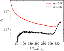
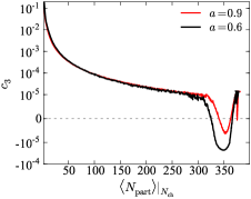
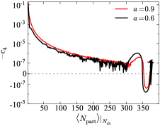
Figure 5: Same as Fig. 1 but for different values of parameter $a$ of Eq. (15). Instead of $a=0.75$ we use $a=0.6$ black lines, and $a=0.9$ red lines.

Before we conclude, we want to mention that:

• Although our minimal model fails to reproduce the measured data, we consider it as a better baseline for low energies than the Poisson distribution, which is typically used. It respects baryon number conservation, and contains the effect of participant fluctuations.

• Although we achieved a qualitative agreement with the observed two-particle correlations, the details do matter. This is demonstrated in Fig. 5. There we vary the parameter $a$ of Eq. (15) from its standard value of $a=0.75$ to $a=0.6$ and $a=0.9$ and plot the resulting couplings $c_{2}$, $c_{3}$, and $c_{4}$. While the three- and four-particle couplings are hardly changed, the two-particle couplings exhibit strong sensitivity on the dependence of the number of charged particles on $N_{\text{part}}$. This dependence can only and should be further constrained by the charged particle distribution, which, however, is not yet publicly available for the STAR measurements.

• Collective stopping or a possible first-order phase transition may lead to clustering of protons at midrapidity. As we pointed out above, by taking this clustering into account it is possible to qualitatively understand the STAR data for the multi-particle correlation functions.

• It would be interesting to measure mixed correlations of fourth order. For example a correlation $C_{3,1}$ between three protons and one produced particle, such as anti-proton or pion may be useful (see the appendix of Ref. Bzdak et al. (2016b) for the relevant formulas). If these mixed correlations, or rather couplings $c_{3,1}$, to avoid trivial sensitivity to the number of particles, are as large as the four-proton coupling $c_{4}$ it would rule out collective stopping and provide evidence for a possible first-order phase transition, as speculated in Sec. IV.

• In this paper we have concentrated on the lowest energy, $\sqrt{s}=7.7{\rm\,GeV}$. Our basic model equally applies to higher energies as long as one can ignore pair production, which is probably still the case at $\sqrt{s}=19.6{\rm\,GeV}$. There, the observed correlations are more or less in agreement with our basic model, subject to the aforementioned uncertainty related to the distribution of the number of charged particles.

In conclusion, the observed large four-proton correlation exhibited in the preliminary STAR data at $\sqrt{s}=7.7$ GeV cannot be explained by a combination of independent baryon stopping, participant fluctuations, and baryon-number conservation. However, more speculative, though not necessarily unrealistic, scenarios involving the “collective” stopping of multiple baryons, may be able to explain the large part of the observed correlation structure. Therefore, it is important to test these ideas by, e.g., measuring mixed correlations. However, given the present analysis and the vary large positive value for the four-proton correlation, $C_{4}$, observed in the preliminary STAR data, it is very difficult to imagine a scenario which explains the data without employing some kind of cluster formation. If these clusters originate from collective stopping, a possible first order phase transition Skokov and Voskresensky (2009a, b); Steinheimer and Randrup (2012); Steinheimer et al. (2014), or some final state effect, remains to be seen, however.

Appendix A General independent source model

Here we generalize our Eqs. (10,11,12) for any independent sources of protons (see also Pumplin (1994)).

Suppose we have $v$ independent sources of protons distributed according to $G(v)$ and each source produces protons according to $p(n_{i})$. The distribution of measured protons in a given rapidity bin $\Delta y$ is given by

$$P(N)=\sum\limits_{v}G(v)\sum_{n_{1},...,n_{v}}p(n_{1})p(n_{2})\cdots p(n_{v})\delta_{n_{1}+...+n_{v}-N}.$$ (29)

We note that this formula is quite general and the only assumption we make is that each source decides on its own how many particles it produces. The generating function reads

$$H(z) = \sum\nolimits_{N}P(N)z^{N}$$ (30)

$$= \sum\nolimits_{v}G(v)\left[\sum\nolimits_{n_{1}}p(n_{1})z^{n_{1}}\right]^{v}$$

$$= \sum\nolimits_{v}G(v)[H_{1}(z)]^{v},$$

where $H_{1}(z)$ is the generating function for a single source.

To calculate correlation functions we use

$$C(z) = \ln\left[H(z)\right]$$ (31)

$$= \ln\left[\sum\nolimits_{v}G(v)e^{v\ln\left[H_{1}(z)\right]}\right]$$

$$= \ln\left[\sum\nolimits_{v}G(v)e^{vC_{1}(z)}\right],$$

where $C_{1}(z)$ characterizes correlations from a single source.

We have

$$C(1)=C_{1}(1)=0;\quad\frac{dC(z)}{dz}|_{z=1}=\left\langle N\right\rangle;\quad\frac{dC_{1}(z)}{dz}|_{z=1}=\left\langle n_{1}\right\rangle=\frac{\left\langle N\right\rangle}{\left\langle v\right\rangle},$$ (32)

where $\left\langle n_{1}\right\rangle$ is the average number of protons from a single source, $\left\langle v\right\rangle$ is the average numbers of sources and $\left\langle N\right\rangle$ is the average number of observed protons.

Calculating derivatives we have for the couplings:

$$c_{2} = \frac{c_{2}^{(1\text{ source})}}{\left\langle v\right\rangle}+\frac{\langle\left[v-\left\langle v\right\rangle\right]^{2}\rangle}{\left\langle v\right\rangle^{2}},$$ (33)

$$c_{3} = \frac{c_{3}^{(1\text{ source})}}{\left\langle v\right\rangle^{2}}+3c_{2}^{(1\text{ source})}\frac{\langle\left[v-\left\langle v\right\rangle\right]^{2}\rangle}{\left\langle v\right\rangle^{3}}+\frac{\langle\left[v-\left\langle v\right\rangle\right]^{3}\rangle}{\left\langle v\right\rangle^{3}},$$ (34)

where $c_{2}^{(1\text{ source})}$ and $c_{3}^{(1\text{ source})}$ are the couplings for a single source. We note that even even if we have only $2$-particle correlations from our sources of protons, they contribute to the three-particle correlations because of the fluctuating number of sources.

For $c_{4}$ we obtain

$$c_{4} = \frac{c_{4}^{(1\text{ source})}}{\left\langle v\right\rangle^{3}}+3\left[c_{2}^{(1\text{ source})}\right]^{2}\frac{\langle\left[v-\left\langle v\right\rangle\right]^{2}\rangle}{\left\langle v\right\rangle^{4}}+6c_{2}^{(1\text{ source})}\frac{\langle\left[v-\left\langle v\right\rangle\right]^{3}\rangle}{\left\langle v\right\rangle^{4}}+$$ (35)

$$4c_{3}^{(1\text{ source})}\frac{\langle\left[v-\left\langle v\right\rangle\right]^{2}\rangle}{\left\langle v\right\rangle^{4}}+\frac{\langle\left[v-\left\langle v\right\rangle\right]^{4}\rangle-3\langle\left[v-\left\langle v\right\rangle\right]^{2}\rangle^{2}}{\left\langle v\right\rangle^{4}}.$$

The above formulas are valid for any independent sources of protons. To obtain Eqs. (10,11,12) from Sec. III we note that the sources of protons are the wounded nucleons themselves. As explained in Sec. III, a wounded nucleon appears in our rapidity bin as a proton with probability $p$ or it does not appear with probability $1-p$. In this case the multiplicity distribution of protons from a single source is given by

$$p(n)=\left\{\begin{array}[]{c}1-p\text{\quad for\quad}n=0\\ p\quad\text{for\quad}n=1\end{array}\right.,$$ (36)

and the generating function for a single source is given by

$$H_{1}(z)=\sum\nolimits_{n}p(n)z^{n}=1-p+pz,$$ (37)

which is a known function for binomial distribution. Following Eqs. (3,5) we have

$$c_{2}^{(1\text{ source})}=-1,\quad c_{3}^{(1\text{ source})}=2,\quad c_{4}^{(1\text{ source})}=-6.$$ (38)

Substituting the above values to Eqs. (33,34,35) and putting $v=N_{\text{part}}$, we obtain Eqs. (10,11,12).