bbm \optbbold
Adaptive nonparametric drift estimation for diffusion processes using Faber-Schauder expansions
Abstract
We consider the problem of nonparametric estimation of the drift of a continuously observed one-dimensional diffusion with periodic drift. Motivated by computational considerations, van der Meulen et al., (2014) defined a prior on the drift as a randomly truncated and randomly scaled Faber-Schauder series expansion with Gaussian coefficients. We study the behaviour of the posterior obtained from this prior from a frequentist asymptotic point of view. If the true data generating drift is smooth, it is proved that the posterior is adaptive with posterior contraction rates for the -norm that are optimal up to a log factor. Contraction rates in -norms with are derived as well.
1 Introduction
Assume continuous time observations from a diffusion process defined as (weak) solution to the stochastic differential equation (sde)
| (1) |
Here is a Brownian Motion and the drift is assumed to be a real-valued measurable function on the real line that is -periodic and square integrable on . The assumed periodicity implies that we can alternatively view the process as a diffusion on the circle. This model has been used for dynamic modelling of angles, see for instance Pokern, (2007) and Hindriks, (2011).
We are interested in nonparametric adaptive estimation of the drift. This problem has recently been studied by multiple authors. Spokoiny, (2000) proposed a locally linear smoother with a data-driven bandwidth choice that is rate adaptive with respect to for all and optimal up to a log factors. Interestingly, the result is non-asymptotic and does not require ergodicity. Dalalyan and Kutoyants, (2002) and Dalalyan, (2005) consider ergodic diffusions and construct estimators that are asymptotically minimax and adaptive under Sobolev smoothness of the drift. Their results were extended to the multidimensional case by Strauch, (2015).
In this paper we focus on Bayesian nonparametric estimation, a paradigm that has become increasingly popular over the past two decades. An overview of some advances of Bayesian nonparametric estimation for diffusion processes is given in van Zanten, (2013).
The Bayesian approach requires the specification of a prior. Ideally, the prior on the drift is chosen such that drawing from the posterior is computationally efficient while at the same time ensuring that the resulting inference has good theoretical properties. which is quantified by a contraction rate. This is a rate for which we can shrink balls around the true parameter value, while maintaining most of the posterior mass. More formally, if is a semimetric on the space of drift functions, a contraction rate is a sequence of positive numbers for which the posterior mass of the balls converges in probability to as , under the law of with drift . For a general discussion on contraction rates, see for instance Ghosal et al., (2000) and Ghosal and van der Vaart, (2007).
For diffusions, the problem of deriving optimal posterior convergence rates has been studied recently under the additional assumption that the drift integrates to zero, . In Papaspiliopoulos et al., (2012) a mean zero Gaussian process prior is proposed together with an algorithm to sample from the posterior. The precision operator (inverse covariance operator) of the proposed Gaussian process is given by , where is the one-dimensional Laplacian, is the identity operator, and . A first consistency result was shown in Pokern et al., (2013).
In van Waaij and van Zanten, (2016) it was shown that this rate result can be improved upon for a slightly more general class of priors on the drift. More specifically, in this paper the authors consider a prior which is defined as
| (2) |
where , are the standard Fourier series basis functions, is a sequence of independent standard normally distributed random variables and is positive. It is shown that when and are fixed and is assumed to be -Sobolev smooth, then the optimal posterior rate of contraction, , is obtained. Note that this result is nonadaptive, as the regularity of the prior must match the regularity of . For obtaining optimal posterior contraction rates for the full range of possible regularities of the drift, two options are investigated: endowing either or with a hyperprior. Only the second option results in the desired adaptivity over all possible regularities.
While the prior in (2) (with additional prior on ) has good asymptotic properties, from a computational point of view the infinite series expansion is inconvenient. Clearly, in any implementation this expansion needs to be truncated. Random truncation of a series expansion is a well known method for defining priors in Bayesian nonparametrics, see for instance Shen and Ghosal, (2015). Exactly this idea was exploited in van der Meulen et al., (2014), where the prior is defined as the law of the random function
| (3) |
where the functions constitute the Faber-Schauder basis (see fig. 1).

These functions feature prominently in the Lévy-Ciesielski construction of Brownian motion (see for instance (Bhattacharya and Waymire,, 2007, paragraph 10.1)). The prior coefficients are equipped with a Gaussian distribution, and the truncation level and the scaling factor are equipped with independent priors. Truncation in absence of scaling increases the apparent smoothness of the prior (as illustrated for deterministic truncation by example 4.5 in van der Vaart and van Zanten, (2008)), whereas scaling by a number decreases the apparent smoothness. (Scaling with a number only increases the apparent smoothness to a limited extent, see for example Knapik et al., (2011).)
The simplest type of prior is obtained by taking the coefficients independent. We do however also consider the prior that is obtained by first expanding a periodic Ornstein-Uhlenbeck process into the Faber-Schauder basis, followed by random scaling and truncation. We will explain that specific stationarity properties of this prior make it a natural choice.
Draws from the posterior can be computed using a reversible jump Markov Chain Monte Carlo (MCMC) algorithm (cf. van der Meulen et al., (2014)). For both types of priors, fast computation is facilitated by leveraging inherent sparsity properties stemming from the compact support of the functions . In the discussion of van der Meulen et al., (2014) it was argued that inclusion of both the scaling and random truncation in the prior is beneficial. However, this claim was only supported by simulations results.
In this paper we support this claim theoretically by proving adaptive contraction rates of the posterior distribution in case the prior (3) is used. We start from a general result in van der Meulen et al., (2006) on Brownian semimartingale models, which we adapt to our setting. Here we take into account that as the drift is assumed to be one-periodic, information accumulates in a different way compared to (general) ergodic diffusions. Subsequently we verify that the resulting prior mass, remaining mass and entropy conditions appearing in this adapted result are satisfied for the prior defined in equation (3). An application of our results shows that if the true drift function is -Besov smooth, , then by appropriate choice of the variances of , as well as the priors on and , the posterior for the drift contracts at the rate around the true drift in the -norm. Up to the log factor this rate is minimax-optimal (See for instance (Kutoyants,, 2004, Theorem 4.48)). Moreover, it is adaptive: the prior does not depend on . In case the true drift has Besov-smoothness greater than or equal to , our method guarantees contraction rates equal to essentially (corresponding to ). A further application of our results shows that for -norms we obtain contraction rate , up to log-factors.
The paper is organised as follows. In the next section we give a precise definition of the prior. In section 3 a general contraction result for the class of diffusion processes considered here is derived. Our main result on posterior contraction for -norms with is presented in section 4. Many results of this paper concern general properties of the prior and their application is not confined to drift estimation of diffusion processes. To illustrate this, we show in section 5 how these results can easily be adapted to nonparametric regression and nonparametric density estimation. Proofs are gathered in section 6. The appendix contains a couple of technical results.
2 Prior construction
2.1 Model and posterior
Let
be the space of square integrable -periodic functions.
Lemma 1.
If then the SDE eq. 1 has a unique weak solution.
The proof is in section 6.1.
For , let denote the law of the process generated by eq. 1 when is replaced by . If denotes the law of when the drift is zero, then is absolutely continuous with respect to with Radon-Nikodym density
| (4) |
Given a prior on and path from (1), the posterior is given by
| (5) |
where is Borel set of . These assertions are verified as part of the proof of 3.
2.2 Motivating the choice of prior
We are interested in randomly truncated, scaled series priors that simultaneously enable a fast algorithm for obtaining draws from the posterior and enjoy good contraction rates.
To explain what we mean by the first item, consider first a prior that is a finite series prior. Let denote basis functions and a mean zero Gaussian random vector with precision matrix . Assume that the prior for is given by . By conjugacy, it follows that , where ,
| (6) |
for , cf. (van der Meulen et al.,, 2014, Lemma 1). The matrix is referred to as the Grammian. From these expressions it follows that it is computationally advantageous to exploit compactly supported basis functions. Whenever and have nonoverlapping supports, we have . Depending on the choice of such basis functions, the Grammian will have a specific sparsity structure (a set of index pairs such that , independently of .) This sparsity structure is inherited by as long as the sparsity structure of the prior precision matrix matches that of .
In the next section we make a specific choice for the basis functions and the prior precision matrix .
2.3 Definition of the prior
Define the “hat” function by . The Faber-Schauder basis functions are given by
We define our prior as in (3) with Gaussian coefficients and , where the truncation level and the scaling factor are equipped with (hyper)priors. We extend periodically if we want to consider as function on the real line. If we identify the double index in (3) with the single index , then we can write . Let
We say that belongs to level if . Thus both and belong to level 0, which is convenient for notational purposes. For levels the basis functions are per level orthogonal with essentially disjoint support. Define for
Let and define its finite-dimensional restriction by . If we denote , and assume that is multivariate normally distributed with mean zero and covariance matrix , then the prior has the following hierarchy
| (7) | ||||
| (8) | ||||
| (9) |
Here, we use to denote the joint distribution of .
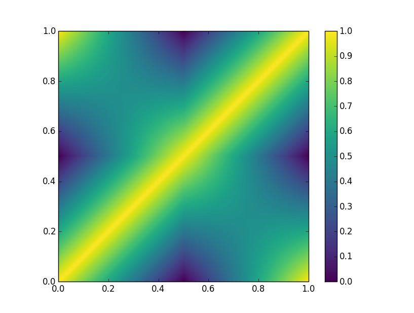
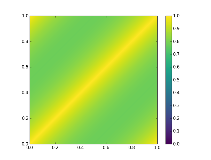
We will consider two choices of priors for the sequence Our first choice consists of taking independent Gaussian random variables. If the coefficients are independent with standard deviation , the random draws from this prior are scaled piecewise linear interpolations on a dyadic grid of a Brownian bridge on plus the random function The choice of is motivated by the fact that in this case is independent of .
We construct this second type of prior as follows. For , define to be the cyclically stationary and centred Ornstein-Uhlenbeck process. This is a periodic Gaussian process with covariance kernel
| (10) |
This process is cyclically stationary, that is, the covariance only depends on and . It is the unique Gaussian and Markovian prior with continuous periodic paths with this property. This makes the cyclically stationary Ornstein-Uhlenbeck prior an appealing choice which respects the symmetries of the problem.
Each realisation of is continuous and can be extended to a periodic function on . Then can be represented as an infinite series expansion in the Faber-Schauder basis:
| (11) |
Finally by scaling by and truncating at we obtain from the second choice of prior on the drift function . Visualisations of the covariance kernels for first prior (Brownian bridge type) and for the second prior (periodic Ornstein-Uhlenbeck process prior with parameter ) are shown in fig. 2 (for and ).
2.4 Sparsity structure induced by choice of
Conditional on and , the posterior of is Gaussian with precision matrix (here is the Grammian corresponding to using all basis functions up to and including level ).
If the coefficients are independent it is trivial to see that the precision matrix does not destroy the sparsity structure of , as defined in (6). This is convenient for numerical computations. The next lemma details the situation for periodic Ornstein-Uhlenbeck processes.
Lemma 2.
Let be defined as in equation (10)
- 1.
-
2.
The entries of the covariance matrix of the random Gaussian coefficients and , , satisfy the following bounds: and for and ,
and and for
The proof is given in section 6.2. By the first part of the lemma, also this prior does not destroy the sparsity structure of the . The second part asserts that while the off-diagonal entries of are not zero, they are of smaller order than the diagonal entries, quantifying that the covariance matrix of the coefficients in the Schauder expansion is close to a diagonal matrix.
3 Posterior contraction for diffusion processes
The main result in van der Meulen et al., (2006) gives sufficient conditions for deriving posterior contraction rates in Brownian semimartingale models. The following theorem is an adaptation and refinement of Theorem 2.1 and Lemma 2.2 of van der Meulen et al., (2006) for diffusions defined on the circle. We assume observations , where Let be a prior on (which henceforth may depend on ) and choose measurable subsets (sieves) . Define the balls
The -covering number of a set for a semimetric , denoted by , is defined as the minimal number of -balls of radius needed to cover the set . The logarithm of the covering number is referred to as the entropy.
The following theorem characterises the rate of posterior contraction for diffusions on the circle in terms of properties of the prior.
Theorem 3.
Suppose is a sequence of positive numbers such that is bounded away from zero. Assume that there is a constant such that for every there is a measurable set and for every there is a constant such that for big enough
| (12) | ||||
| (13) | ||||
| and | ||||
| (14) | ||||
Then for every
| and for big enough, | ||||
| (15) | ||||
Equations (12), (13) and (14) are referred to as the entropy condition, small ball condition and remaining mass condition of 3 respectively. The proof of this theorem is in section 6.3.
4 Theorems on posterior contraction rates
The main result of this section, 9 characterises the frequentist rate of contraction of the posterior probability around a fixed parameter of unknown smoothness using the truncated series prior from section 2.
We make the following assumption on the true drift function.
Assumption 4.
The true drift can be expanded in the Faber-Schauder basis, and there exists a such that
| (16) |
Note that we use a slightly different symbol for the norm, as we denote the -norm by .
Remark 5.
If , then 4 on is equivalent to assuming to be -Besov smooth. It follows from the definition of the basis functions that
Therefore it follows from equations (4.72) (with ) and (4.73) (with ) in combination with equation (4.79) (with ) in Giné and Nickl, (2016), section 4.3, that is equivalent to the -norm of for .
If , then –Hölder smoothness and –smoothness coincide (cf. Proposition 4.3.23 in Giné and Nickl, (2016)).
Assumption 6.
The covariance matrix satisfies one of the following conditions:
-
(A)
For fixed , and for .
-
(B)
There exists and with independent from , such that for all
In particular the second assumption if fulfilled by the prior defined by eq. 10 if and any .
Assumption 7.
The prior on the truncation level satisfies for some positive constants ,
| (17) |
For the prior on the scaling we assume existence of constants , and with such that
| (18) |
The prior on can be defined as , where is Poisson distributed. Equation 18 is satisfied for a whole range of distributions, including the popular family of inverse gamma distributions. Since the inverse gamma prior on decays polynomially (lemma 17), condition (A2) of Shen and Ghosal, (2015) is not satisfied and hence their posterior contraction results cannot be applied to our prior. We obtain the following result for our prior.
Theorem 8.
The following theorem is obtained by applying these bounds to 3 after taking .
This means that when the true parameter is from a rate is obtained that is optimal possibly up to a log factor. When then is in particular in the space for every small positive , and therefore converges with rate essentially .
When a different function is used, defined on a compact interval of and the basis elements are defined by ; forcing them to be 1-periodic. Then 9 and derived results for applications still holds provided and when for a fixed and the smoothness assumptions on are changed accordingly. A finite number of basis elements can be added or redefined as long as they are 1-periodic.
It is easy to see that our results imply posterior convergences rates in weaker -norms, with the same rate. When the -norm is stronger than the -norm. We apply ideas of Knapik and Salomond, (2014) to obtain rates for stronger -norms.
Theorem 10.
These rates are similar to the rates obtained for the density estimation in Giné and Nickl, (2011). However our proof is less involved. Note that we have only consistency for .
5 Applications to nonparametric regression and density estimation
Our general results also apply to other models. The following results are obtained for satisfying 4 and the prior satisfying assumptions 6 and 7.
5.1 Nonparametric regression model
As a direct application of the properties of the prior shown in the previous section, we obtain the following result for a nonparametric regression problem. Assume
| (22) |
with independent Gaussian observation errors . When we apply Ghosal and van der Vaart, (2007), example 7.7 to 8 we obtain, for every ,
as and (in a similar way as in 10) for every ,
as .
5.2 Density estimation
Let us consider independent observations with where is an unknown density on relative to the Lebesgue measure. Let denote the space of densities on relative to the Lebesgue measure. The natural distance for densities is the Hellinger distance defined by
6 Proofs
6.1 Proof of lemma 1
Since conditions (ND) and (LI) of (Karatzas and Shreve,, 1991, theorem 5.15) hold, the SDE eq. 1 has a unique weak solution up to an explosion time.
Assume without loss of generality that . Define and for the random times
By periodicity of drift and the Markov property the random variables are independent and identically distributed.
Note that
and hence non-explosion follows from almost surely. The latter holds true since with positive probability, which is clear from the continuity of diffusion paths.
6.2 Proof of lemma 2
Proof of the first part. For the proof we introduce some notation: for any , we write if . The set of indices become a lattice with partial order , and by we denote the supremum. Identify with and similarly with .
For , denote by the time points in corresponding to the maxima of . Without loss of generality assume . We have if and only if the interiors of the supports of and are disjoint. In that case
| (23) |
The values of can be found by the midpoint displacement technique. The coefficients are given by , and for
As is a Gaussian process, the vector is mean-zero Gaussian, say with (infinite) precision matrix . Now if there exists a set such that for which conditional on , are are independent.
Define and
The set determine the process at all times , .
Now and are conditionally independent given by (23) and the Markov property of the nonperiodic Ornstein-Uhlenbeck process.
The result follows since .
Lemma 11.
Let . If
Proof.
Without loss of generality assume that . With and
The result follows from and scaling both sides with . ∎
Proof of the second part. Denote by , the support of and respectively and let and but for , let . , and , and . Note that the covariance matrix of and has eigenvalues and and is strictly positive definite.
By midpoint displacement, , and .
Assume without loss of generality . Define to be the halfwidth of the smaller interval, so that . Then
Consider three cases:
-
1.
The entries on diagonal, ;
-
2.
The interiors of the supports of and are non-overlapping;
-
3.
The support of is contained in the support of .
Case 1. By elementary computations for ,
As and under the assumption the last display can be bounded by
Hence .
Case 2. Necessarily . By twofold application of lemma 11
| (24) |
Using the convexity of we obtain the bound
| (25) |
for . Note that is convex on , from which we derive . Using this bound, and the fact that for ,
| (26) |
which can be easily seen from a plot, that
Case 3.
For , with or with , using eq. 26, we obtain
| (27) |
Write and . A simple computation then shows
The derivative of is nonnegative, for hence is increasing and so . Note that and . Maximising over gives and and therefore .
It follows that
For the other terms we derive the following bounds. Write
Now is decreasing for and convex and positive for . In both case we can bound by its value at the endpoints and . Using that we obtain and . So .
Using the bound eq. 25 and we obtain
6.3 Proof of 3
A general result for deriving contraction rates for Brownian semi-martingale models was proved in van der Meulen et al., (2006). Theorem 3 follows upon verifying the assumptions of this result for the diffusion on the circle. These assumptions are easily seen to boil down to:
-
1.
For every and the measures and are equivalent.
-
2.
The posterior as defined in equation eq. 5 is well defined.
-
3.
Define the (random) Hellinger semimetric on by
(28) There are constants for which
We start by verifying the third condition. Recall that the local time of the process is defined as the random process which satisfies
For every measurable function for which the above integrals are defined. Since we are working with 1-periodic functions, we define the periodic local time by
Note that is continuous with probability one. Hence the support of is compact with probability one. Since is only positive on the support of , it follows that the sum in the definition of has only finitely many nonzero terms and is therefore well defined. For a one-periodic function we have
provided the involved integrals exists. It follows from (Schauer and van Zanten,, 2017, Theorem 5.3) that converges to a positive deterministic function only depending only on and which is bounded away from zero and infinity. Since the Hellinger distance can be written as
it follows that the third assumption is satisfied with .
Conditions 1 and 2 now follow by arguing precisely as in lemmas A.2 and 3.1 of van Waaij and van Zanten, (2016) respectively (the key observation being that the convergence result of also holds when is nonzero, which is assumed in that paper).
The stated result follows from Theorem 2.1 in van der Meulen et al., (2006) (taking in their paper).
6.4 Proof of 8 with 6 (A)
The proof proceeds by verifying the conditions of theorem 3. By 4 the true drift can be represented as . For , define its truncated version by
6.4.1 Small ball probability
For choose an integer with
| (29) |
For notational convenience we will write instead of in the remainder of the proof. By lemma 16 we have . Therefore
which implies
Let denotes the probability density of . For any , we have
| (30) |
where
and and are taken from 7. For sufficiently small, we have by the second part of 7
By choice of and the first part of 7, there exists a positive constant such that
for sufficiently small.
For lower bounding the middle term in equation (30), we write
which implies
This gives the bound
By choice of the we have for all is standard normally distributed and hence
where the inequality follows from lemma 18. The third term can be further bounded as we have
Hence
| (31) |
For and we will now derive bounds on the first three terms on the right of eq. 31. For sufficiently small we have and then inequality (29) implies
Bounding the first term on the RHS of (31). For sufficiently small, we have
where is a positive constant.
Bounding the second term on the RHS of (31). For sufficiently small, we have
The final inequality is immediate in case , else if suffices to verify that the exponent is non-negative under the assumption .
Bounding the third term on the RHS of (31). For sufficiently small, in case we have
In case we have
as the exponent of is positive under the assumption .
Hence for small enough, we have
As we get
We conclude that the right hand side of eq. 30 is bounded below by , for some positive constant and sufficiently small .
6.4.2 Entropy and remaining mass conditions
For denote by the linear space spanned by and , , and define
Proposition 12.
For any
where .
Proof.
We follow (van der Meulen et al.,, 2006, §3.2.2). Choose such that . Define
For each , let be a minimal -net with respect to the max-distance on and let be a minimal -net with respect to the max-distance on . Hence, if , then there exists a such that .
Take arbitrary: . Let , where and (for ). We have
This can be bounded by by an appropriate choice of the coefficients in . In that case we obtain that . This implies
The asserted bound now follows upon choosing .
∎
Proposition 13.
There exists a constant a positive constant such that
Proof.
We can now finish the proof for the entropy and remaining mass conditions. Choose to be the smallest integer so that , where is a constant, and set . The entropy bound then follows directly from 13.
For the remaining mass condition, using 7, we obtain
and note that the constant can be made arbitrarily big by choosing big enough.
6.5 Proof of 8 under 6 (B)
We start with a lemma.
Lemma 14.
Assume there exists and with independent from , such that for all ,
| (33) | ||||
| (34) |
Let (so the right-lower submatrix of ). Then for all
where is the diagonal matrix with .
Proof.
In the following the summation are over . Trivially, . By the first inequality
On the other hand
At the first inequality we used the second part of of (33). The second inequality follows upon including the diagonal. By Cauchy-Schwarz, this can be further bounded by
where the final inequality follows from . The result follows by combining the derived inequalities. ∎
We continue with the proof of 8. Write as block matrix
with a -matrix, and , defined accordingly. By lemma 2
Define the -matrix
where is the -identity matrix. It is easy to see that is positive definite.
When is positive definite, then it follows from the Cholesky decomposition that is positive definite, where positive definite.
Note
where
Therefore
Now consider . By lemma 2 and the bound on and choosing in the definition of small enough, under the assumption that ,
and for . Therefore by lemma 14 is positive definite with diagonal matrix with diagonal entries .
It follows that . This implies that the small ball probabilities and the mass outside a sieve behave similar under 6(B) as when the are independent normally distributed with zero mean and variance . As this case corresponds to 6(A) with for which posterior contraction has already been established, the stated contraction rate under 6(B) follows from Anderson’s lemma (lemma 19).
6.6 Proof of 10: convergence in stronger norms
The linear embedding operator is a well-defined injective continuous operator for all . Its inverse is easily seen to be a densely defined, closed unbounded linear operator. Following Knapik and Salomond, (2014) we define the modulus of continuity as
Theorem 2.1 of Knapik and Salomond, (2014) adapted to our case is
Theorem 15 (Knapik and Salomond, (2014)).
Let and be a prior on such that
for measurable sets . Assume that for any positive sequence
then
Note that the sieves which we define in section 6.4.2 have by eq. 15 the property By lemmas 21 and 23, the modulus of continuity satisfies , for all , (assume ), and the result follows.
Appendix A Lemmas used in the proofs
Lemma 16.
Proof.
This follows from
∎
Lemma 17.
If then for any ,
Proof.
This follows from
∎
Lemma 18.
Let , and .Then
Proof.
Note that
and
thus hence
Now the elementary bound gives
∎
Lemma 19 (Anderson’s lemma).
Define a partial order on the space of -matrices () by setting when is positive definite. If and independently with , then for all symmetric convex sets
Proof.
See Anderson, (1955). ∎
Lemma 20.
Let
Then
Proof.
Note that , and and inductively, for , , hence . ∎
Lemma 21.
Let as in section 6.4.2. Then
Proof.
Let be nonzero. Note that for any constant ,
Hence, we may and do assume that . Furthermore, since the and norm of and are the same, we also assume that is nonnegative.
Let be a global maximum of . Clearly . Since is a linear interpolation between the points , we may also assume that is of the form . We consider two cases
-
(i)
,
-
(ii)
.
In case (i) we have that , for all . In case (ii) , for all . Hence, in both cases,
Thus
uniformly over all nonzero . ∎
Lemma 22.
Let be positive numbers. Then
Proof.
Suppose that the lemma is not true, so there are positive such that,
Hence, both terms on the right-hand-side are negative. In particular, this means for the first term that . For the second term this gives . These two inequalities cannot hold simultaneously and we have reached a contradiction. ∎
Lemma 23.
Let and as in section 6.4.2. Then for ,
Proof.
Let . Just as in proof of lemma 21 we may assume that is nonnegative and . Hence
Note that
Hence, by repeatedly applying lemma 22
Note that is a linear interpolation between the points .
Now study affine functions which are positive. A maximum of is attained in either or . Without lose of generality it is attained in . Using scaling in a later stadium of the proof, we assume for the moment that . Hence . Note that
When , . Now consider ,
Let then and . Hence
Note that for a constant and a function ,
Let
Hence has -norm one and
The maximum is attained for , then
Hence
and the result follows, using that and that for ,
∎
Appendix B Acknowledgement
This work was partly supported by the Netherlands Organisation for Scientific Research (NWO) under the research programme “Foundations of nonparametric Bayes procedures”, 639.033.110 and by the ERC Advanced Grant “Bayesian Statistics in Infinite Dimensions”, 320637.
References
- Anderson, (1955) Anderson, T. W. (1955). The integral of a symmetric unimodal function over a symmetric convex set and some probability inequalities. Proc. Amer. Math. Soc., 6:170–176.
- Bhattacharya and Waymire, (2007) Bhattacharya, R. and Waymire, E. (2007). A Basic Course in Probability Theory. Universitext. Springer New York.
- Dalalyan, (2005) Dalalyan, A. (2005). Sharp adaptive estimation of the drift function for ergodic diffusions. Ann. Statist., 33(6):2507–2528.
- Dalalyan and Kutoyants, (2002) Dalalyan, A. S. and Kutoyants, Y. A. (2002). Asymptotically efficient trend coefficient estimation for ergodic diffusion. Math. Methods Statist., 11(4):402–427 (2003).
- Ghosal et al., (2000) Ghosal, S., Ghosh, J. K., and van der Vaart, A. W. (2000). Convergence rates of posterior distributions. Ann. Statist., 28(2):500–531.
- Ghosal and van der Vaart, (2007) Ghosal, S. and van der Vaart, A. W. (2007). Convergence rates of posterior distributions for noniid observations. Ann. Statist., 35(1):192–223.
- Giné and Nickl, (2011) Giné, E. and Nickl, R. (2011). Rates of contraction for posterior distributions in -metrics, . Ann. Statist., 39(6):2883–2911.
- Giné and Nickl, (2016) Giné, E. and Nickl, R. (2016). Mathematical foundations of infinite-dimensional statistical models. Cambridge Series in Statistical and Probabilistic Mathematics. Cambridge University Press.
- Hindriks, (2011) Hindriks, R. (2011). Empirical dynamics of neuronal rhythms. PhD thesis, Vrije Universiteit Amsterdam.
- Karatzas and Shreve, (1991) Karatzas, I. and Shreve, S. E. (1991). Brownian motion and stochastic calculus, volume 113 of Graduate Texts in Mathematics. Springer-Verlag, New York, second edition.
- Knapik and Salomond, (2014) Knapik, B. and Salomond, J.-B. (2014). A general approach to posterior contraction in nonparametric inverse problems. Bernoulli.
- Knapik et al., (2011) Knapik, B. T., van der Vaart, A. W., and van Zanten, J. H. (2011). Bayesian inverse problems with Gaussian priors. Ann. Statist., 39(5):2626–2657.
- Kutoyants, (2004) Kutoyants, Y. A. (2004). Statistical inference for ergodic diffusion processes. Springer, New York.
- Papaspiliopoulos et al., (2012) Papaspiliopoulos, O., Pokern, Y., Roberts, G. O., and Stuart, A. M. (2012). Nonparametric estimation of diffusions: a differential equations approach. Biometrika, 99(3):511.
- Pokern, (2007) Pokern, Y. (2007). Fitting Stochastic Differential Equations to Molecular Dynamics Data. PhD thesis, University of Warwick.
- Pokern et al., (2013) Pokern, Y., Stuart, A. M., and van Zanten, J. H. (2013). Posterior consistency via precision operators for Bayesian nonparametric drift estimation in SDEs. Stochastic Processes and their Applications, 123(2):603 – 628.
- Schauer and van Zanten, (2017) Schauer, M. and van Zanten, J. H. (2017). Uniform central limit theorems for additive functionals of diffusions on the circle. In preparation.
- Shen and Ghosal, (2015) Shen, W. and Ghosal, S. (2015). Adaptive Bayesian procedures using random series priors. Scandinavian Journal of Statistics, 42(4):1194–1213.
- Spokoiny, (2000) Spokoiny, V. G. (2000). Adaptive drift estimation for nonparametric diffusion model. Ann. Statist., 28(3):815–836.
- Strauch, (2015) Strauch, C. (2015). Sharp adaptive drift estimation for ergodic diffusions: the multivariate case. Stochastic Process. Appl., 125(7):2562–2602.
- van der Meulen et al., (2014) van der Meulen, F. H., Schauer, M., and van Zanten, J. H. (2014). Reversible jump MCMC for nonparametric drift estimation for diffusion processes. Comput. Statist. Data Anal., 71:615–632.
- van der Meulen et al., (2006) van der Meulen, F. H., van der Vaart, A. W., and van Zanten, J. H. (2006). Convergence rates of posterior distributions for Brownian semimartingale models. Bernoulli, 12(5):863–888.
- van der Vaart and van Zanten, (2008) van der Vaart, A. W. and van Zanten, J. H. (2008). Rates of contraction of posterior distributions based on Gaussian process priors. Ann. Statist., 36(3):1435–1463.
- van Waaij and van Zanten, (2016) van Waaij, J. and van Zanten, H. (2016). Gaussian process methods for one-dimensional diffusions: Optimal rates and adaptation. Electron. J. Statist., 10(1):628–645.
- van Zanten, (2013) van Zanten, J. H. (2013). Nonparametric Bayesian methods for one-dimensional diffusion models. Mathematical biosciences, 243(2):215–222.