A Dirichlet problem for the Laplace operator in a domain with a small hole close to the boundary

Abstract

We study the Dirichlet problem in a domain with a small hole close to the boundary. To do so, for each pair ${\boldsymbol{\varepsilon}}=(\varepsilon_{1},\varepsilon_{2})$ of positive parameters, we consider a perforated domain $\Omega_{{\boldsymbol{\varepsilon}}}$ obtained by making a small hole of size $\varepsilon_{1}\varepsilon_{2}$ in an open regular subset $\Omega$ of $\mathbb{R}^{n}$ at distance $\varepsilon_{1}$ from the boundary $\partial\Omega$. As $\varepsilon_{1}\to 0$, the perforation shrinks to a point and, at the same time, approaches the boundary. When ${\boldsymbol{\varepsilon}}\to(0,0)$, the size of the hole shrinks at a faster rate than its approach to the boundary. We denote by $u_{\boldsymbol{\varepsilon}}$ the solution of a Dirichlet problem for the Laplace equation in $\Omega_{{\boldsymbol{\varepsilon}}}$. For a space dimension $n\geq 3$, we show that the function mapping ${\boldsymbol{\varepsilon}}$ to $u_{\boldsymbol{\varepsilon}}$ has a real analytic continuation in a neighborhood of $(0,0)$. By contrast, for $n=2$ we consider two different regimes: ${\boldsymbol{\varepsilon}}$ tends to $(0,0)$, and $\varepsilon_{1}$ tends to $0$ with $\varepsilon_{2}$ fixed. When ${\boldsymbol{\varepsilon}}\to(0,0)$, the solution $u_{\boldsymbol{\varepsilon}}$ has a logarithmic behavior; when only $\varepsilon_{1}\to 0$ and $\varepsilon_{2}$ is fixed, the asymptotic behavior of the solution can be described in terms of real analytic functions of $\varepsilon_{1}$. We also show that for $n=2$, the energy integral and the total flux on the exterior boundary have different limiting values in the two regimes. We prove these results by using functional analysis methods in conjunction with certain special layer potentials.

Keywords: Dirichlet problem; singularly perturbed perforated domain; Laplace operator; real analytic continuation in Banach space; asymptotic expansion

2010 Mathematics Subject Classification: 35J25; 31B10; 45A05; 35B25; 35C20.

1 Introduction

Elliptic boundary value problems in domains where a small part has been removed arise in the study of mathematical models for bodies with small perforations or inclusions, and are of interest not only for their mathematical aspects, but also for their applications to elasticity, heat conduction, fluid mechanics, and so on. They play a central role in the treatment of inverse problems (see, e.g., Ammari and Kang [1]) and in the computation of the so-called ‘topological derivative’, which is a fundamental tool in shape and topological optimization (see, e.g., Novotny and Sokołowsky [33]). Owing to the difference in size between the small removed part and the whole domain, the application of standard numerical methods requires the use of highly nonhomogeneous meshes that often lead to inaccuracy and instability. This difficulty can be overcome and the validity of the chosen numerical strategies can be guaranteed only if adequate theoretical studies are first conducted on the problem.

In this paper, we consider the case of the Dirichlet problem for the Laplace equation in a domain with a small hole ‘moderately close’ to the boundary, i.e., a hole that approaches the outer boundary of the domain at a certain rate, while shrinking to a point at a faster rate. In two-dimensional space, we also consider the case where the size of the hole and its distance from the boundary are comparable. It turns out that the two types of asymptotic behavior in this setup are different: the first case gives rise to logarithmic behavior, whereas the second one generates a real analytic continuation result. Additionally, the energy integral and the total flux of the solution on the outer boundary may have different limiting values.

We begin by describing the geometric setting of our problem. We take $n\in\mathbb{N}\setminus\{0,1\}$ and, without loss of generality, we place the problem in the upper half space, which we denote by $\mathbb{R}^{n}_{+}$. More precisely, we define

$$\mathbb{R}^{n}_{+}\equiv\{\mathsf{x}=(x_{1},\dots,x_{n})\in\mathbb{R}^{n}\;:\;x_{n}>0\}\,.$$

We note that the boundary $\partial\mathbb{R}^{n}_{+}$ coincides with the hyperplane $x_{n}=0$. Then we fix a domain $\Omega$ such that

$$\Omega \mathbb{R}^{n}_{+} {\mathscr{C}}^{1,\alpha} H_{1}$$ is an open bounded connected subset of of class , ()

where $\alpha\in]0,1[$ is a regularity parameter. The definition of functions and sets of the usual Schauder classes ${\mathscr{C}}^{k,\alpha}$ ($k=0,1$) can be found, for example, in Gilbarg and Trudinger [19, §6.2]. We denote by $\partial\Omega$ the boundary of $\Omega$. In this paper, we assume that a part of $\partial\Omega$ is flat and that the hole is approaching it (see Figure 1). This is described by setting

$$\partial_{0}\Omega\equiv\partial\Omega\cap\partial\mathbb{R}^{n}_{+},\qquad\partial_{+}\Omega\equiv\partial\Omega\cap\mathbb{R}^{n}_{+},$$

and assuming that

$$\partial_{0}\Omega 0 \partial\mathbb{R}^{n}_{+} H_{2}$$ is an open neighborhood of in . ()

The set $\Omega$ plays the role of the ‘unperturbed’ domain. To define the hole, we consider another set $\omega$ satisfying the following assumption:

$$\omega \mathbb{R}^{n} {\mathscr{C}}^{1,\alpha} 0\in\omega$$ is a bounded open connected subset of of class such that .

The set $\omega$ represents the shape of the perforation. Then we fix a point

$$\mathsf{p}=(p_{1},\dots,p_{n})\in\mathbb{R}^{n}_{+},$$ (1.1)

and define the inclusion $\omega_{{\boldsymbol{\varepsilon}}}$ by

$$\omega_{{\boldsymbol{\varepsilon}}}\equiv\varepsilon_{1}\mathsf{p}+\varepsilon_{1}\varepsilon_{2}\omega\,,\qquad\forall{\boldsymbol{\varepsilon}}\equiv(\varepsilon_{1},\varepsilon_{2})\in\mathbb{R}^{2}\,.$$

We adopt the following notation. If ${\boldsymbol{\varepsilon}}^{\prime}\equiv(\varepsilon_{1}^{\prime},\varepsilon_{2}^{\prime}),{\boldsymbol{\varepsilon}}^{\prime\prime}\equiv(\varepsilon_{1}^{\prime\prime},\varepsilon_{2}^{\prime\prime})\in\mathbb{R}^{2}$, then we write ${\boldsymbol{\varepsilon}}^{\prime}\leq{\boldsymbol{\varepsilon}}^{\prime\prime}$ (respectively, ${\boldsymbol{\varepsilon}}^{\prime}<{\boldsymbol{\varepsilon}}^{\prime\prime}$) if and only if $\varepsilon_{j}^{\prime}\leq\varepsilon_{j}^{\prime\prime}$ (respectively, $\varepsilon_{j}^{\prime}<\varepsilon_{j}^{\prime\prime}$), for $j=1,2$, and denote by $]{\boldsymbol{\varepsilon}}^{\prime},{\boldsymbol{\varepsilon}}^{\prime\prime}[$ the open rectangular domain of ${\boldsymbol{\varepsilon}}\in\mathbb{R}^{2}$ such that ${\boldsymbol{\varepsilon}}^{\prime}<{\boldsymbol{\varepsilon}}<{\boldsymbol{\varepsilon}}^{\prime\prime}$. We also set ${\boldsymbol{0}}\equiv(0,0)$. Then it is easy to verify that there is ${{\boldsymbol{\varepsilon}}^{\rm ad}}\in]0,+\infty[^{2}$ such that

$$\overline{\omega_{{\boldsymbol{\varepsilon}}}}\subseteq\Omega,\qquad\forall{\boldsymbol{\varepsilon}}\in{]{{\boldsymbol{0}}},{{\boldsymbol{\varepsilon}}^{\rm ad}}[}.$$

In addition, since we are interested in the case where the vector $(\varepsilon_{1},\varepsilon_{1}\varepsilon_{2})$ is close to ${\boldsymbol{0}}$, we may assume without loss of generality that

$$\varepsilon_{1}^{\rm ad}<1 1<\varepsilon_{2}^{\rm ad}<1/\varepsilon_{1}^{\rm ad}$$ and .

Hence, $\varepsilon_{1}\varepsilon_{2}<1$ for all ${\boldsymbol{\varepsilon}}\in{]{{\boldsymbol{0}}},{{\boldsymbol{\varepsilon}}^{\rm ad}}[}$. This technical condition allows us to deal with the function $1/\log(\varepsilon_{1}\varepsilon_{2})$ as in Section 4, and to consider the case where $\varepsilon_{2}=1$ in Section 5.

In a certain sense, ${]{{\boldsymbol{0}}},{{\boldsymbol{\varepsilon}}^{\rm ad}}[}$ is a set of admissible parameters for which we can define the perforated domain $\Omega_{{\boldsymbol{\varepsilon}}}$ obtained by removing from the unperturbed domain $\Omega$ the closure $\overline{\omega}_{{\boldsymbol{\varepsilon}}}$ of $\omega_{{\boldsymbol{\varepsilon}}}$, i.e.,

$$\Omega_{{\boldsymbol{\varepsilon}}}\equiv\Omega\setminus\overline{\omega_{{\boldsymbol{\varepsilon}}}},\qquad\forall{\boldsymbol{\varepsilon}}\in{]{{\boldsymbol{0}}},{{\boldsymbol{\varepsilon}}^{\rm ad}}[}.$$

We remark that, for all ${\boldsymbol{\varepsilon}}\in{]{{\boldsymbol{0}}},{{\boldsymbol{\varepsilon}}^{\rm ad}}[}$, $\Omega_{{\boldsymbol{\varepsilon}}}$ is a bounded connected open domain of class ${\mathscr{C}}^{1,\alpha}$ with boundary $\partial\Omega_{{\boldsymbol{\varepsilon}}}$ consisting of two connected components: $\partial\Omega$ and $\partial\omega_{{\boldsymbol{\varepsilon}}}=\varepsilon_{1}\mathsf{p}+\varepsilon_{1}\varepsilon_{2}\partial\omega$. The distance of the hole $\omega_{{\boldsymbol{\varepsilon}}}$ from the boundary $\partial\Omega$ is controlled by $\varepsilon_{1}$, while its size is controlled by the product $\varepsilon_{1}\varepsilon_{2}$. Clearly, as the pair ${\boldsymbol{\varepsilon}}\in{]{{\boldsymbol{0}}},{{\boldsymbol{\varepsilon}}^{\rm ad}}[}$ approaches the singular value $(0,\varepsilon_{2}^{*})$, both the size of the cavity and its distance from the boundary $\partial\Omega$ tend to $0$. If $\varepsilon_{2}^{*}=0$, then the ratio of the size of the hole to its distance from the boundary tends to $0$, and we can say that the size tends to zero ‘faster’ than the distance. If, instead, $\varepsilon_{2}^{*}>0$, then the size of the hole and its distance from the boundary tend to zero at the same rate. Figure 1 illustrates our geometric setting.

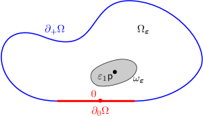
Figure 1: Geometrical setting.

On the ${\boldsymbol{\varepsilon}}$-dependent domain $\Omega_{{\boldsymbol{\varepsilon}}}$, for ${\boldsymbol{\varepsilon}}\in{]{{\boldsymbol{0}}},{{\boldsymbol{\varepsilon}}^{\rm ad}}[}$ fixed we now consider the Dirichlet problem

$$\begin{cases}\Delta u(\mathsf{x})=0,&\forall\mathsf{x}\in\Omega_{{\boldsymbol{\varepsilon}}}\,,\\ u(\mathsf{x})=g^{\mathrm{o}}(\mathsf{x}),&\forall\mathsf{x}\in\partial\Omega\,,\\ u(\mathsf{x})=g^{\mathrm{i}}\Big{(}\frac{\mathsf{x}-\varepsilon_{1}\mathsf{p}}{\varepsilon_{1}\varepsilon_{2}}\Big{)},&\forall\mathsf{x}\in\partial\omega_{{\boldsymbol{\varepsilon}}}\,,\end{cases}$$ (1.2)

where $g^{\mathrm{o}}\in{\mathscr{C}}^{1,\alpha}(\partial\Omega)$ and $g^{\mathrm{i}}\in{\mathscr{C}}^{1,\alpha}(\partial\omega)$ are prescribed functions. As is well known, (1.2) has a unique solution in ${\mathscr{C}}^{1,\alpha}(\overline{\Omega_{{\boldsymbol{\varepsilon}}}})$. To emphasize the dependence of this solution on ${\boldsymbol{\varepsilon}}$, we denote it by $u_{\boldsymbol{\varepsilon}}$. The aim of this paper is to investigate the behavior of $u_{\boldsymbol{\varepsilon}}$ when the parameter ${\boldsymbol{\varepsilon}}=(\varepsilon_{1},\varepsilon_{2})$ approaches the singular value ${\boldsymbol{0}}\equiv(0,0)$. In two-dimensional space we also consider the case where $\varepsilon_{1}\to 0$ with $\varepsilon_{2}>0$ fixed, and show that this leads to a specific asymptotic behavior. Namely, in such regime, there are no logarithmic terms appearing in the asymptotic behavior of the solution, in contrast with what happens when ${\boldsymbol{\varepsilon}}=(\varepsilon_{1},\varepsilon_{2})\to(0,0)$ in dimension two (cf. Subsections 1.3.2 and 1.3.3 below). In higher dimension, instead, the case where $\varepsilon_{1}\to 0$ with $\varepsilon_{2}>0$ fixed does not present specific differences and the tools developed for analyzing the situation when ${\boldsymbol{\varepsilon}}=(\varepsilon_{1},\varepsilon_{2})\to(0,0)$ can be exploited by keeping $\varepsilon_{2}>0$ “frozen”. Then the corresponding results on the macroscopic and microscopic behavior would follow. For this reason, we confine here to analyze the case where $\varepsilon_{1}\to 0$ with $\varepsilon_{2}>0$ fixed only in dimension two.

We remark that every point $\mathsf{x}\in\Omega$ stays in $\Omega_{{\boldsymbol{\varepsilon}}}$ for $\varepsilon_{1}$ sufficiently close to $0$. Accordingly, if we fix a point $\mathsf{x}\in\Omega$, then $u_{\boldsymbol{\varepsilon}}(\mathsf{x})$ is well defined for $\varepsilon_{1}$ sufficiently small and we may ask the following question:

What can be said about the map $${\boldsymbol{\varepsilon}}\mapsto u_{\boldsymbol{\varepsilon}}(\mathsf{x}) {\boldsymbol{\varepsilon}}>{\boldsymbol{0}} {\bf 0}$$ for close to ? (1.3)

We mention that here we do not consider the case where $\varepsilon_{2}$ is close to $0$ and $\varepsilon_{1}$ remains positive. This case corresponds to a boundary value problem in a domain with a hole that collapses to a point in its interior, and has already been studied in the literature.

1.1 Explicit computation on a toy problem

To explain our results, we first consider a two-dimensional test problem that has an explicit solution. We denote by $\mathcal{B}(\mathsf{x},\rho)$ the ball centered at $\mathsf{x}$ and of radius $\rho$, take a function $g^{\mathrm{i}}\in{\mathscr{C}}^{1,\alpha}(\partial\mathcal{B}(0,1))$, and, for ${\boldsymbol{\varepsilon}}\in]{\boldsymbol{0}},(1,1)[$, consider the following Dirichlet problem in the perforated half space $\mathbb{R}^{2}_{+}\setminus\mathcal{B}((0,\varepsilon_{1}),\varepsilon_{1}\varepsilon_{2})$:

$$\begin{cases}\Delta u_{\boldsymbol{\varepsilon}}(\mathsf{x})=0,&\forall\mathsf{x}\in\mathbb{R}^{2}_{+}\setminus\mathcal{B}((0,\varepsilon_{1}),\varepsilon_{1}\varepsilon_{2})\\ u_{\boldsymbol{\varepsilon}}(\mathsf{x})=0,&\forall\mathsf{x}\in\partial\mathbb{R}^{2}_{+},\\ u_{\boldsymbol{\varepsilon}}(\mathsf{x})=g^{\mathrm{i}}\Big{(}\frac{\mathsf{x}-\varepsilon_{1}\mathsf{p}}{\varepsilon_{1}\varepsilon_{2}}\Big{)},&\forall\mathsf{x}\in\partial\mathcal{B}((0,\varepsilon_{1}),\varepsilon_{1}\varepsilon_{2}),\\ \lim_{\mathsf{x}\to\infty}u_{\boldsymbol{\varepsilon}}(\mathsf{x})=0\,,\end{cases}$$ (1.4)

where $\mathsf{p}=(0,1)$. We also consider the conformal map

$$\varphi_{a}:\leavevmode\nobreak\ z\mapsto\cfrac{z-ia}{z+ia}\,,$$

with inverse

$$\varphi^{-1}_{a}:\leavevmode\nobreak\ z\mapsto-ia\ \cfrac{z+1}{z-1}\,.$$

When $a\neq 0$ is real, $\varphi_{a}$ maps the real axis onto the unit circle. Moreover, if

$$a({\boldsymbol{\varepsilon}})=a(\varepsilon_{1},\varepsilon_{2})=\varepsilon_{1}\sqrt{1-\varepsilon_{2}^{2}}\,,$$

then $\varphi_{a({\boldsymbol{\varepsilon}})}$ maps the circle centered at $(0,\varepsilon_{1})$ and of radius $\varepsilon_{1}\varepsilon_{2}$ to the circle centered at the origin and of radius

$$\rho(\varepsilon_{2})=\sqrt{\cfrac{1-\sqrt{1-\varepsilon_{2}^{2}}}{1+\sqrt{1+\varepsilon_{2}^{2}}}}\,.$$

We note that the maps $a:\ (\varepsilon_{1},\varepsilon_{2})\mapsto a({\boldsymbol{\varepsilon}})$ and $\rho:\ \varepsilon_{2}\mapsto\rho(\varepsilon_{2})$ are analytic. We mention that a similar computation is performed in Ben Hassen and Bonnetier [2] for the case of two balls removed from an infinite medium.

Since harmonic functions are transformed into harmonic functions by a conformal map, we can now transfer problem (1.4) onto the annular domain $\mathcal{B}(0,1)\setminus\mathcal{B}(0,\rho(\varepsilon_{2}))$ by means of the map $\varphi_{a({\boldsymbol{\varepsilon}})}$ and see that the unknown function $\underline{u}_{\boldsymbol{\varepsilon}}=u_{\boldsymbol{\varepsilon}}\circ\varphi^{-1}_{a({\boldsymbol{\varepsilon}})}$ satisfies

$$\begin{cases}\Delta\underline{u}_{\boldsymbol{\varepsilon}}=0,&\mbox{ in }\mathcal{B}(0,1)\setminus\mathcal{B}(0,\rho(\varepsilon_{2})),\\ \underline{u}_{\boldsymbol{\varepsilon}}=0,&\mbox{ on }\partial\mathcal{B}(0,1),\\ \underline{u}_{\boldsymbol{\varepsilon}}(z)=\underline{g}^{\mathrm{i}}_{\,{\boldsymbol{\varepsilon}}}(\arg{z}),&\mbox{ for all }z\in\partial\mathcal{B}(0,\rho(\varepsilon_{2})),\end{cases}$$

and the new boundary condition

$$\underline{g}^{\mathrm{i}}_{\,{\boldsymbol{\varepsilon}}}(\theta)=g^{\mathrm{i}}\left(-\cfrac{i}{\varepsilon_{2}}\ \left(\sqrt{1-\varepsilon_{2}^{2}}\ \cfrac{\rho(\varepsilon_{2})e^{i\theta}+1}{\rho(\varepsilon_{2})e^{i\theta}-1}\ +1\right)\right),\qquad\forall\theta\in[0,2\pi[.$$

To obtain the analytic expression of the solution, we expand $\underline{g}^{\mathrm{i}}_{\,{\boldsymbol{\varepsilon}}}$ in the Fourier series

$$\underline{g}^{\mathrm{i}}_{\,{\boldsymbol{\varepsilon}}}(\theta)=a_{0}(\underline{g}^{\mathrm{i}}_{\,{\boldsymbol{\varepsilon}}})+\sum_{k\geq 1}a_{k}(\underline{g}^{\mathrm{i}}_{\,{\boldsymbol{\varepsilon}}})\cos{k\theta}+b_{k}(\underline{g}^{\mathrm{i}}_{\,{\boldsymbol{\varepsilon}}})\sin{k\theta},$$

so that, in polar coordinates,

$$\underline{u}_{\boldsymbol{\varepsilon}}(r,\theta)=a_{0}(\underline{g}^{\mathrm{i}}_{\,{\boldsymbol{\varepsilon}}}){\frac{\log r}{\log\rho(\varepsilon_{2})}}+\sum_{k\geq 1}\left(a_{k}(\underline{g}^{\mathrm{i}}_{\,{\boldsymbol{\varepsilon}}})\cos{k\theta}+b_{k}(\underline{g}^{\mathrm{i}}_{\,{\boldsymbol{\varepsilon}}})\sin{k\theta}\right)\frac{r^{k}-r^{-k}}{\rho(\varepsilon_{2})^{k}-\rho(\varepsilon_{2})^{-k}}.$$

We can then recover $u_{\boldsymbol{\varepsilon}}$ by computing $u_{\boldsymbol{\varepsilon}}=\underline{u}_{\boldsymbol{\varepsilon}}\circ\varphi_{a({\boldsymbol{\varepsilon}})}$. To this end, we remark that in polar coordinates we have $\varphi_{a({\boldsymbol{\varepsilon}})}(\mathsf{x})=r_{\boldsymbol{\varepsilon}}(\mathsf{x})e^{i\theta_{\boldsymbol{\varepsilon}}(\mathsf{x})}$, with

$$r_{\boldsymbol{\varepsilon}}(\mathsf{x})=\left|\cfrac{x_{1}+ix_{2}-ia({\boldsymbol{\varepsilon}})}{x_{1}+ix_{2}+ia({\boldsymbol{\varepsilon}})}\right|,\qquad\theta_{\boldsymbol{\varepsilon}}(\mathsf{x})=\arg\left(\cfrac{x_{1}+ix_{2}-ia({\boldsymbol{\varepsilon}})}{x_{1}+ix_{2}+ia({\boldsymbol{\varepsilon}})}\right).$$

As an example, if we assume that $g^{\mathrm{i}}=1$, then the solution of (1.4) is

$$u_{\boldsymbol{\varepsilon}}(\mathsf{x})=\frac{\log r_{\boldsymbol{\varepsilon}}(\mathsf{x})}{\log\rho(\varepsilon_{2})}\ =\ \cfrac{\log{\left(x_{1}^{2}+\left(x_{2}-\varepsilon_{1}\sqrt{1-\varepsilon_{2}^{2}}\right)^{2}\right)}\ -\ \log{\left(x_{1}^{2}+\left(x_{2}+\varepsilon_{1}\sqrt{1-\varepsilon_{2}^{2}}\right)^{2}\right)}}{\log{\left(1-\sqrt{1-\varepsilon_{2}^{2}}\right)}-\log{\left(1+\sqrt{1+\varepsilon_{2}^{2}}\right)}}.$$ (1.5)

We note that for any fixed $\mathsf{x}\in\mathbb{R}^{2}_{+}$ and $\varepsilon_{1}$, $\varepsilon_{2}$ positive and sufficiently small, the map ${\boldsymbol{\varepsilon}}\mapsto u_{\boldsymbol{\varepsilon}}(\mathsf{x})$ is analytic. When ${\boldsymbol{\varepsilon}}\to{\boldsymbol{0}}$, the function $u_{\boldsymbol{\varepsilon}}$ tends to $0$ with a main term of order $\varepsilon_{1}|\log\varepsilon_{2}|^{-1}$. In addition, for $\varepsilon_{2}>0$ fixed, the map $\varepsilon_{1}\mapsto u_{\boldsymbol{\varepsilon}}(\mathsf{x})$ has an analytic continuation around $\varepsilon_{1}=0$.

In what follows, we intend to prove similar results also for problem (1.2), and thus answer the question (1.3) by investigating the analyticity properties of the function ${\boldsymbol{\varepsilon}}\mapsto u_{\boldsymbol{\varepsilon}}(\mathsf{x})$. Furthermore, instead of evaluating $u_{\boldsymbol{\varepsilon}}$ at a point $\mathsf{x}$, we consider its restriction to suitable subsets of $\Omega$ and the restriction of the rescaled function $\mathsf{X}\mapsto u_{\boldsymbol{\varepsilon}}(\varepsilon_{1}\mathsf{p}+\varepsilon_{1}\varepsilon_{2}\mathsf{X})$ to suitable open subsets of $\mathbb{R}^{2}\setminus\overline{\omega}$. This permits us to study functionals related to $u_{\boldsymbol{\varepsilon}}$, such as the energy integral and the total flux on $\partial\Omega$. Our main results are described in Subsection 1.3, in the next subsection instead we present our strategy.

1.2 Methodology: the functional analytic approach

In the literature, most of the papers dedicated to the analysis of problems with small holes employ expansion methods to provide asymptotic approximations of the solution. As an example, we mention the method of matching asymptotic expansions proposed by Il’in (see, e.g., [20, 21, 22]), the compound asymptotic expansion method of Maz’ya, Nazarov, and Plamenevskij [30] and of Kozlov, Maz’ya, and Movchan [23], and the mesoscale asymptotic approximations presented by Maz’ya, Movchan, and Nieves [29, 31]. We also mention the works of Bonnaillie-Noël, Lacave, and Masmoudi [7], Chesnel and Claeys [8], and Dauge, Tordeux, and Vial [16]. Boundary value problems in domains with moderately close small holes have been analyzed by means of multiple scale asymptotic expansions by Bonnaillie-Noël, Dambrine, Tordeux, and Vial [5, 6], Bonnaillie-Noël and Dambrine [3], and Bonnaillie-Noël, Dambrine, and Lacave [4].

A different technique, proposed by Lanza de Cristoforis and referred to as a ‘functional analytic approach’, aims at expressing the dependence of the solution on perturbation in terms of real analytic functions. This approach has so far been applied to the study of various elliptic problems, including problems with nonlinear conditions. For problems involving the Laplace operator we refer the reader to the papers of Lanza de Cristoforis (see, e.g., [24, 25]), Dalla Riva and Musolino (see, e.g., [11, 12, 13]), and Dalla Riva, Musolino, and Rogosin [15], where the computation of the coefficients of the power series expansion of the resulting analytic maps is reduced to the solution of certain recursive systems of boundary integral equations.

In the present paper, we plan to exploit the functional analytic approach to represent the map that associates ${\boldsymbol{\varepsilon}}$ with (suitable restrictions of) the solution $u_{\boldsymbol{\varepsilon}}$ in terms of real analytic maps with values in convenient Banach spaces of functions and of known elementary functions of $\varepsilon_{1}$ and $\varepsilon_{2}$ (for the definition of real analytic maps in Banach spaces, see Deimling [17, p. 150]). Then we can recover asymptotic approximations similar to those obtainable from the expansion methods. For example, if we know that, for $\varepsilon_{1}$ and $\varepsilon_{2}$ small and positive, the function in (1.3) equals a real analytic function defined in a whole neighborhood of $(0,0)$, then we know that such a map can be expanded in a power series for $\varepsilon_{1}$ and $\varepsilon_{2}$ small, and that a truncation of this series is an approximation of the solution.

To conclude the presentation of our strategy, we would like to comment on some novel techniques that we bring into the functional analytic approach for the analysis of our problem. First, we describe how the functional analytic approach ‘normally’ operates on a boundary value problem defined on a domain that depends on a parameter ${\boldsymbol{\varepsilon}}$ and degenerates in some sense as ${\boldsymbol{\varepsilon}}$ tends to a limiting value $\bf 0$. The initial step consists in applying potential theory techniques to transform the boundary value problem into a system of boundary integral equations. Then, possibly after some suitable manipulation, this system is written as a functional equation of the form ${\mathfrak{L}}[{\boldsymbol{\varepsilon}},{\boldsymbol{\mu}}]=0$, where ${\mathfrak{L}}$ is a (nonlinear) operator acting from an open subset of a Banach space ${\mathscr{R}}\times{\mathscr{B}}_{1}$ to another Banach space ${\mathscr{B}}_{2}$. Here ${\mathscr{R}}$ is a neighborhood of $\bf 0$ and the Banach spaces ${\mathscr{B}}_{1}$ and ${\mathscr{B}}_{2}$ are usually the direct product of Schauder spaces on the boundaries of certain fixed domains. The next step is to apply the implicit function theorem to the equation ${\mathfrak{L}}[{\boldsymbol{\varepsilon}},{\boldsymbol{\mu}}]=0$ in order to understand the dependence of ${\boldsymbol{\mu}}$ on ${\boldsymbol{\varepsilon}}$. Then we can deduce the dependence of the solution of the original boundary value problem on ${\boldsymbol{\varepsilon}}$.

The strategy adopted in this paper differs from the standard application of the functional analytic approach in two ways.

• The first one concerns the potential theory used to transform the problem into a system of integral equations. To take care of the special geometry of the problem, instead of the classical layer potentials for the Laplace operator, we construct layer potentials where the role of the fundamental solution is taken by the Dirichlet Green’s function of the upper half space. Since the hole collapses on $\partial\mathbb{R}^{n}_{+}\cap\partial\Omega$ as ${\boldsymbol{\varepsilon}}$ tends to $\bf 0$, such a method allows us to eliminate the integral equation defined on the part of the boundary of $\Omega_{{\boldsymbol{\varepsilon}}}$ where the boundary of the hole and the exterior boundary interact for ${\boldsymbol{\varepsilon}}={\bf 0}$. In Section 2, we collect a number of general results on such special layer potentials. We remark that if the union of $\Omega$ and its reflection with respect to $\partial\mathbb{R}^{n}_{+}$ is a regular domain, then there is no need to introduce special layer potentials and the problem may be analyzed by means of a technique based on the functional analytic approach and on a reflection argument (see Costabel, Dalla Riva, Dauge, and Musolino [10]). However, under our assumption, the union of $\Omega$ and its reflection with respect to $\partial\mathbb{R}^{n}_{+}$ produces an edge on $\partial\mathbb{R}^{n}_{+}$ and, thus, is not a regular domain.

• By using the special layer potentials mentioned above, we can transform problem (1.2) into an equation of the form ${\mathfrak{L}}[{\boldsymbol{\varepsilon}},{\boldsymbol{\mu}}]=0$, where the operator ${\mathfrak{L}}$ acts from an open set ${]-{{\boldsymbol{\varepsilon}}^{\rm ad}},{{\boldsymbol{\varepsilon}}^{\rm ad}}[}\times{\mathscr{B}}_{1}$ into a Banach space ${\mathscr{B}}_{2}$ whose construction is, in a certain sense, artificial. ${\mathscr{B}}_{2}$ is the direct product of a Schauder space and the image of a specific integral operator (see Propositions 2.11 and 3.1). In this context, we have to be particularly careful to check that the image of ${\mathfrak{L}}$ is actually contained in such a Banach space ${\mathscr{B}}_{2}$, and that ${\mathfrak{L}}$ is a real analytic operator (see Proposition 3.1). We remark that this step is instead quite straightforward in previous applications of the functional analytic approach (see, e.g., [13, Prop. 5.4]). Once this work is completed, we are ready to use the implicit function theorem and deduce the dependence of the solution on ${\boldsymbol{\varepsilon}}$.

1.3 Main results

To perform our analysis, in addition to ($H_{1}$)–($H_{2}$) we also assume that $\Omega$ satisfies the condition

$$\overline{\partial_{+}\Omega} \mathbb{R}^{n} {\mathscr{C}}^{1,\alpha} H_{3}$$ is a compact submanifold with boundary of of class . ()

In the two-dimensional case, this condition takes the form

$$\overline{\partial_{0}\Omega} \partial\mathbb{R}^{2}_{+} H_{3}$$ is a finite union of closed disjoint intervals in . ()

In particular, we note that assumption ($H_{3}$) implies the existence of linear and continuous extension operators $E^{k,\alpha}$ from ${\mathscr{C}}^{k,\alpha}(\overline{\partial_{+}\Omega})$ to ${\mathscr{C}}^{k,\alpha}(\partial\Omega)$, for $k=0,1$ (cf. Lemma 2.17 below). This allows us to change from functions defined on $\partial_{+}\Omega$ to functions defined on $\partial\Omega$ (and viceversa), preserving their regularity.

To prove our analyticity result, we consider a regularity condition on the Dirichlet datum around the origin, namely

there exists $$r_{0}>0 g^{\mathrm{o}}_{|\mathcal{B}(0,r_{0})\cap\partial_{0}\Omega} H_{4}$$ such that the restriction is real analytic. ()

As happens for the solution to the Dirichlet problem in a domain with a small hole ‘far’ from the boundary, we show that $u_{\boldsymbol{\varepsilon}}$ converges as $\varepsilon_{1}\to 0$ to a function $u_{0}$ that is the unique solution in ${\mathscr{C}}^{1,\alpha}(\overline{\Omega})$ of the following Dirichlet problem in the unperturbed domain $\Omega$:

$$\begin{cases}\Delta u=0&\mbox{ in }\Omega\,,\\ u=g^{\mathrm{o}}&\mbox{ on }\partial\Omega\,.\\ \end{cases}$$

We note that $u_{0}$ is harmonic, and therefore analytic, in the interior of $\Omega$. This fact is useful in the study of the Dirichlet problem in a domain with a hole that shrinks to an interior point of $\Omega$. If, instead, the hole shrinks to a point on the boundary, as it does in this paper, then we have to introduce condition ($H_{4}$) in order to ensure that $u_{0}$ has an analytic (actually, harmonic) extension around the limit point. Indeed, by ($H_{4}$) and a classical argument based on the Cauchy-Kovalevskaya Theorem, we can prove the following assertion (cf. B).

Proposition 1.1.

There is $r_{1}\in]0,r_{0}]$ and a function $U_{0}$ from $\overline{\mathcal{B}(0,r_{1})}$ to $\mathbb{R}$ such that $\mathcal{B}^{+}(0,r_{1})\subseteq\Omega$ and

$$\begin{cases}\Delta U_{0}=0&\mbox{ in }\mathcal{B}(0,r_{1}),\\ U_{0}=u_{0}&\mbox{ in }\overline{\mathcal{B}^{+}(0,r_{1})},\end{cases}$$

where $\mathcal{B}^{+}(0,r)=\mathcal{B}(0,r)\cap\mathbb{R}^{n}_{+}$.

Then, possibly shrinking $\varepsilon_{1}^{\rm ad}$, we may assume that

$$\varepsilon_{1}\mathsf{p}+\varepsilon_{1}\varepsilon_{2}\overline{\omega}\subseteq\mathcal{B}(0,r_{1}),\qquad\forall{\boldsymbol{\varepsilon}}\in{]-{{\boldsymbol{\varepsilon}}^{\rm ad}},{{\boldsymbol{\varepsilon}}^{\rm ad}}[}\,.$$ (1.6)

We now give our answers to question (1.3). We remark that, instead of the evaluation of $u_{\boldsymbol{\varepsilon}}$ at a point $\mathsf{x}$, we consider its restriction to a suitable subset $\Omega^{\prime}$ of $\Omega$.

1.3.1 The case ${\boldsymbol{\varepsilon}}\to{\boldsymbol{0}}$ in spaces of dimension $n\geq 3$

For ${\boldsymbol{\varepsilon}}\to{\boldsymbol{0}}$, the question (1.3) is answered differently when $n\geq 3$ and $n=2$. If $n\geq 3$, the statement is easier.

Theorem 1.2.

Let $\Omega^{\prime}$ be an open subset of $\Omega$ such that $0\notin\overline{\Omega^{\prime}}$. There are ${\boldsymbol{\varepsilon}}^{\prime}\in{]{{\boldsymbol{0}}},{{\boldsymbol{\varepsilon}}^{\rm ad}}[}$ with $\overline{\omega_{{\boldsymbol{\varepsilon}}}}\cap\overline{\Omega^{\prime}}=\emptyset$ for all ${\boldsymbol{\varepsilon}}\in{]-{\boldsymbol{\varepsilon}}^{\prime},{\boldsymbol{\varepsilon}}^{\prime}[}$ and a real analytic map ${{\mathfrak{U}}}_{\Omega^{\prime}}$ from ${]-{\boldsymbol{\varepsilon}}^{\prime},{\boldsymbol{\varepsilon}}^{\prime}[}$ to ${\mathscr{C}}^{1,\alpha}(\overline{\Omega^{\prime}})$ such that

$${u_{\boldsymbol{\varepsilon}}}_{|\overline{\Omega^{\prime}}}={{\mathfrak{U}}}_{\Omega^{\prime}}[{\boldsymbol{\varepsilon}}]\qquad\forall{\boldsymbol{\varepsilon}}\in{]{{\boldsymbol{0}}},{\boldsymbol{\varepsilon}}^{\prime}[}\,.$$ (1.7)

Furthermore,

$${{\mathfrak{U}}}_{\Omega^{\prime}}[{\bf 0}]=u_{0|\overline{\Omega^{\prime}}}\,.$$ (1.8)

Theorem 1.2 implies that there are ${\boldsymbol{\varepsilon}}^{\prime\prime}\in]0,{\boldsymbol{\varepsilon}}^{\prime}[$ and a family of functions $\{U_{i,j}\}_{i,j\in\mathbb{N}^{2}}\subseteq{\mathscr{C}}^{1,\alpha}(\overline{\Omega^{\prime}})$ such that

$$u_{{\boldsymbol{\varepsilon}}}(\mathsf{x})=\sum_{i,j=0}^{\infty}U_{i,j}(\mathsf{x})\;\varepsilon_{1}^{i}\varepsilon_{2}^{j}\,,\qquad\forall{\boldsymbol{\varepsilon}}\in]0,{\boldsymbol{\varepsilon}}^{\prime\prime}[\,,\;\mathsf{x}\in\overline{\Omega^{\prime}},$$

with the power series $\sum_{i,j=0}^{\infty}U_{i,j}\;\varepsilon_{1}^{i}\varepsilon_{2}^{j}$ converging in the norm of ${\mathscr{C}}^{1,\alpha}(\overline{\Omega^{\prime}})$ for ${\boldsymbol{\varepsilon}}$ in an open neighborhood of ${\boldsymbol{0}}$. Consequently, one can compute asymptotic approximations for $u_{\boldsymbol{\varepsilon}}$ whose convergence is guaranteed by our preliminary analysis.

A result similar to Theorem 1.2 is expressed in Theorem 3.6 concerning the behavior of $u_{\boldsymbol{\varepsilon}}$ close to the boundary of the hole, namely, for the rescaled function $\mathsf{X}\mapsto u_{\boldsymbol{\varepsilon}}(\varepsilon_{1}\mathsf{p}+\varepsilon_{1}\varepsilon_{2}\,\mathsf{X})$. Later, in Theorems 3.7 and 3.9 we present real analytic continuation results also for the energy integral $\int_{\Omega_{{\boldsymbol{\varepsilon}}}}|\nabla u_{\boldsymbol{\varepsilon}}|^{2}d\mathsf{x}$. In particular, we show that the limiting value of the energy integral for ${\boldsymbol{\varepsilon}}\to{\boldsymbol{0}}$ is the energy of the unperturbed solution $u_{0}$.

1.3.2 The case ${\boldsymbol{\varepsilon}}\to{\boldsymbol{0}}$ in two-dimensional space

Here, we need to introduce a curve $\eta\mapsto{\boldsymbol{\varepsilon}}(\eta)\equiv(\varepsilon_{1}(\eta),\varepsilon_{2}(\eta))$ that describes the values attained by the parameter ${\boldsymbol{\varepsilon}}$ in a specific way. The reason is the presence of the quotient

$$\frac{\log\varepsilon_{1}}{\log(\varepsilon_{1}\varepsilon_{2})},$$ (1.9)

which plays an important role in the description of $u_{\boldsymbol{\varepsilon}}$ for ${\boldsymbol{\varepsilon}}$ small. We remark that the expression (1.9) has no limit as ${\boldsymbol{\varepsilon}}\to{\boldsymbol{0}}$. Therefore, we choose a function $\eta\mapsto{\boldsymbol{\varepsilon}}(\eta)$ from $]0,1[$ to ${]{{\boldsymbol{0}}},{{\boldsymbol{\varepsilon}}^{\rm ad}}[}$ such that

$$\lim_{\eta\to 0^{+}}{\boldsymbol{\varepsilon}}(\eta)={\boldsymbol{0}},$$ (1.10)

and for which

$$\lim_{\eta\to 0^{+}}\frac{\log\varepsilon_{1}(\eta)}{\log(\varepsilon_{1}(\eta)\varepsilon_{2}(\eta))}\quad\text{ exists and equals }\lambda\in[0,1[.$$ (1.11)

It is also convenient to denote by ${\boldsymbol{\delta}}$ the function

$$\begin{array}[]{rcl}{\boldsymbol{\delta}}:\quad]0,1[&\to&\mathbb{R}^{2},\\ \eta&\mapsto&{\boldsymbol{\delta}}(\eta)\equiv\big{(}\delta_{1}(\eta),\delta_{2}(\eta)\big{)}\equiv\biggl{(}\frac{1}{\log\big{(}\varepsilon_{1}(\eta)\varepsilon_{2}(\eta)\big{)}},\frac{\log\varepsilon_{1}(\eta)}{\log\big{(}\varepsilon_{1}(\eta)\varepsilon_{2}(\eta)\big{)}}\biggr{)}\,,\end{array}$$ (1.12)

so that

$$\lim_{\eta\to 0^{+}}{\boldsymbol{\delta}}(\eta)=(0,\lambda)\,.$$

In Section 4, we prove an assertion that describes $u_{{\boldsymbol{\varepsilon}}(\eta)}$ in terms of a real analytic function of four real variables evaluated at $({\boldsymbol{\varepsilon}}(\eta),{\boldsymbol{\delta}}(\eta))$.

Theorem 1.3.

Let $\lambda\in[0,1[$. Let $\Omega^{\prime}$ be an open subset of $\Omega$ with $0\notin\overline{\Omega^{\prime}}$. Then there are ${\boldsymbol{\varepsilon}}^{\prime}\in{]{{\boldsymbol{0}}},{{\boldsymbol{\varepsilon}}^{\rm ad}}[}$, an open neighborhood ${\cal V}_{\lambda}$ of $(0,\lambda)$ in $\mathbb{R}^{2}$, and a real analytic map

$${\mathfrak{U}}_{\Omega^{\prime}}:]-{\boldsymbol{\varepsilon}}^{\prime},{\boldsymbol{\varepsilon}}^{\prime}[\times{\cal V}_{\lambda}\to{\mathscr{C}}^{1,\alpha}(\overline{\Omega^{\prime}}),$$

such that

$$u_{{\boldsymbol{\varepsilon}}(\eta)|\overline{\Omega^{\prime}}}={\mathfrak{U}}_{\Omega^{\prime}}\bigl{[}{\boldsymbol{\varepsilon}}(\eta),{\boldsymbol{\delta}}(\eta)\bigr{]}\,,\qquad\forall\eta\in]0,\eta^{\prime}[\,.$$ (1.13)

The equality in (1.13) holds for all parametrizations $\eta\mapsto{\boldsymbol{\varepsilon}}(\eta)$ from $]0,1[$ to ${]{{\boldsymbol{0}}},{{\boldsymbol{\varepsilon}}^{\rm ad}}[}$ that satisfy (1.10) and (1.11). The function $\eta\mapsto{\boldsymbol{\delta}}(\eta)$ is defined as in (1.12). The pair ${\boldsymbol{\varepsilon}}^{\prime}\in{]{{\boldsymbol{0}}},{{\boldsymbol{\varepsilon}}^{\rm ad}}[}$ is small enough to yield

$$\overline{\omega_{{\boldsymbol{\varepsilon}}}}\cap\overline{\Omega^{\prime}}=\emptyset\,,\qquad\forall{\boldsymbol{\varepsilon}}\in]-{\boldsymbol{\varepsilon}}^{\prime},{\boldsymbol{\varepsilon}}^{\prime}[\,,$$ (1.14)

and $\eta^{\prime}$ can be any number in $]0,1[$ such that

$$\left({\boldsymbol{\varepsilon}}(\eta),{\boldsymbol{\delta}}(\eta)\right)\in]0,{\boldsymbol{\varepsilon}}^{\prime}[\times{\cal V}_{\lambda}\,,\qquad\forall\eta\in]0,\eta^{\prime}[\,.$$

At the singular point $({\boldsymbol{0}},(0,\lambda))$, we have

$${\mathfrak{U}}_{\Omega^{\prime}}[{\boldsymbol{0}},(0,\lambda)]=u_{0|\overline{\Omega^{\prime}}}\,.$$ (1.15)

As a corollary to Theorem 1.3, we can write the solution $u_{{\boldsymbol{\varepsilon}}(\eta)}$ in terms of a power series in $\left({\boldsymbol{\varepsilon}}(\eta),{\boldsymbol{\delta}}(\eta)\right)$ for $\eta$ positive and small. Specifically, there are $\eta^{\prime\prime}\in]0,\eta^{\prime}]$ and a family of functions $\{U_{\boldsymbol{\beta}}\}_{{\boldsymbol{\beta}}\in\mathbb{N}^{4}}\subseteq{\mathscr{C}}^{1,\alpha}(\overline{\Omega^{\prime}})$ such that

$$u_{{\boldsymbol{\varepsilon}}(\eta)}(\mathsf{x})=\sum_{{\boldsymbol{\beta}}\in\mathbb{N}^{4}}U_{\boldsymbol{\beta}}(\mathsf{x})\;\varepsilon_{1}(\eta)^{\beta_{1}}\varepsilon_{2}(\eta)^{\beta_{2}}\delta_{1}(\eta)^{\beta_{3}}(\delta_{2}(\eta)-\lambda)^{\beta_{4}}\qquad\forall\eta\in]0,\eta^{\prime\prime}[\,,\;\mathsf{x}\in\overline{\Omega^{\prime}}\,.$$

Moreover, the power series $\sum_{{\boldsymbol{\beta}}\in\mathbb{N}^{4}}U_{\boldsymbol{\beta}}\;\varepsilon_{1}^{\beta_{1}}\varepsilon_{2}^{\beta_{2}}\delta_{1}^{\beta_{3}}(\delta_{2}-\lambda)^{\beta_{4}}$ converges in the norm of ${\mathscr{C}}^{1,\alpha}(\overline{\Omega^{\prime}})$ for $(\varepsilon_{1},\varepsilon_{2},\delta_{1},\delta_{2})$ in an open neighborhood of $({\boldsymbol{0}},(0,\lambda))$.

We emphasize that the map ${\mathfrak{U}}_{\Omega^{\prime}}$, as well as the coefficients $\{U_{\boldsymbol{\beta}}\}_{{\boldsymbol{\beta}}\in\mathbb{N}^{4}}$, depends on the limiting value $\lambda$, but not on the specific curve ${\boldsymbol{\varepsilon}}(\cdot)$ that satisfies (1.11). A result similar to Theorem 1.3 also holds, which describes the behavior of the solution of problem (1.2) close to the hole (cf. Theorem 4.8), for the energy integral $\int_{\Omega_{\varepsilon}}|\nabla u_{\varepsilon}|^{2}\,d\mathsf{x}$ (cf. Theorem 4.9), and for the total flux through the outer boundary $\int_{\partial\Omega}{\boldsymbol{\mathsf{n}}}_{\Omega}\cdot\nabla u_{\varepsilon}\,d\sigma$ (cf. Theorem 4.10). In particular, we show that the limiting value of the energy integral is

$$\lim_{\eta\to 0}\int_{\Omega_{\varepsilon}}|\nabla u_{{\boldsymbol{\varepsilon}}(\eta)}|^{2}\,d\mathsf{x}=\int_{\Omega}|\nabla u_{0}|^{2}\,d\mathsf{x}+\int_{\mathbb{R}^{2}\setminus\omega}\left|\nabla v_{0}\right|^{2}\,d\mathsf{x},$$ (1.16)

where $v_{0}\in{\mathscr{C}}^{1,\alpha}_{\mathrm{loc}}(\mathbb{R}^{2}\setminus\omega)$ is the unique solution of

$$\left\{\begin{array}[]{ll}\Delta v_{0}=0&\text{in }\mathbb{R}^{2}\setminus\overline{\omega}\,,\\ v_{0}=g^{\mathrm{i}}&\text{on }\partial\omega\,,\\ \sup_{\mathbb{R}^{2}\setminus\omega}|v_{0}|<+\infty\,.&\end{array}\right.$$ (1.17)

In addition, we show that the flux on $\partial\Omega$ satisfies

$$\lim_{\eta\to 0}\int_{\partial\Omega}{\boldsymbol{\mathsf{n}}}_{\Omega}\cdot\nabla u_{{\boldsymbol{\varepsilon}}(\eta)}\,d\sigma=0.$$

Finally, we remark that the functions $\delta_{1}$ and $\delta_{2}$ are not uniquely defined. For example, we may choose

$$\tilde{\delta}_{2}(\eta)\equiv\frac{\log\varepsilon_{2}(\eta)}{\log\big{(}\varepsilon_{1}(\eta)\varepsilon_{2}(\eta)\big{)}}$$

or other similar alternatives instead of $\delta_{2}(\eta)$ (we note that $\tilde{\delta}_{2}(\eta)=1-\delta_{2}(\eta)$). Furthermore, the solution may not depend on the quotient (1.9) if we consider problems with a different geometry. For instance, in the toy problem of Subsection 1.1, the solution (1.5) can be written as an analytic map of three variables evaluated at $(\varepsilon_{1},\varepsilon_{2},({\log\varepsilon_{2}})^{-1})$. As we emphasize in a comment at the end of Subsection 4.1, the reason for this simpler behavior is that in the toy problem we do not have an exterior boundary $\partial_{+}\Omega$. It is worth noting that a quotient similar to (1.9) plays a fundamental role also in the two-dimensional Dirichlet problem with moderately close small holes, which was investigated in [14] and where it was shown that an analog of the limiting value $\lambda$ (cf. (1.11)) appears explicitly in the second term of the asymptotic expansion of the solution.

1.3.3 The case $\varepsilon_{1}\to 0$ with $\varepsilon_{2}>0$ fixed in two-dimensional space

We remark that we may restrict our attention to the problem with $\varepsilon_{2}=1$. Then the generic case of $\varepsilon_{2}=\varepsilon_{2}^{*}\in]0,\varepsilon_{2}^{\rm ad}[$ fixed is obtained by rescaling the reference domain $\omega$ using the factor $\varepsilon_{2}^{*}$. We also remark that the restricted case is a one-parameter problem. Consequently, it is convenient to define ${\varepsilon^{\rm ad}}\equiv\varepsilon_{1}^{\rm ad}$, $\omega_{\varepsilon}\equiv\omega_{\varepsilon_{1},1}$, $\Omega_{\varepsilon}\equiv\Omega_{\varepsilon_{1},1}$, and $u_{\varepsilon}\equiv u_{\varepsilon_{1},1}$ for all $\varepsilon\in{]-{\varepsilon^{\rm ad}},{\varepsilon^{\rm ad}}[}$. The next assertion is proved in Section 5.

Theorem 1.4.

Let $\Omega^{\prime}$ be an open subset of $\Omega$ such that $0\notin\overline{\Omega^{\prime}}$. Then there are $\varepsilon^{\prime}\in]0,\varepsilon_{1}^{\rm ad}[$ such that

$$\overline{\omega_{\varepsilon}}\cap\overline{\Omega^{\prime}}=\emptyset\qquad\forall\varepsilon\in]-\varepsilon^{\prime},\varepsilon^{\prime}[\,$$ (1.18)

and a real analytic map ${\mathfrak{U}}_{\Omega^{\prime}}$ from $]-\varepsilon^{\prime},\varepsilon^{\prime}[$ to ${\mathscr{C}}^{1,\alpha}(\overline{\Omega^{\prime}})$ satisfying

$$u_{\varepsilon|\overline{\Omega^{\prime}}}={\mathfrak{U}}_{\Omega^{\prime}}[\varepsilon],\qquad\forall\varepsilon\in]0,\varepsilon^{\prime}[\,.$$ (1.19)

Furthermore,

$${\mathfrak{U}}_{\Omega^{\prime}}[0]=u_{0|\overline{\Omega^{\prime}}}\,.$$ (1.20)

Theorem 1.4 implies that there are $\varepsilon^{\prime\prime}\in]0,\epsilon^{\prime}[$ and a sequence of functions $\{U_{j}\}_{j\in\mathbb{N}}\subseteq{\mathscr{C}}^{1,\alpha}(\overline{\Omega^{\prime}})$ such that

$$u_{\varepsilon}(\mathsf{x})=\sum_{j=0}^{\infty}U_{j}(\mathsf{x})\,\varepsilon^{j}\qquad\forall\varepsilon\in]0,\varepsilon^{\prime\prime}[\,,\;\mathsf{x}\in\overline{\Omega^{\prime}},$$

with the power series $\sum_{j=0}^{\infty}U_{j}\,\varepsilon^{j}$ converging in the norm of ${\mathscr{C}}^{1,\alpha}(\overline{\Omega^{\prime}})$ for $\varepsilon$ in an open neighborhood of $0$.

A result similar to Theorem 1.4 is also established for the behavior of $u_{\varepsilon}$ near the boundary of the hole (cf. Theorem 5.7), for the energy integral $\int_{\Omega_{\varepsilon}}|\nabla u_{\varepsilon}|^{2}\,d\mathsf{x}$ (cf. Theorem 5.9), and for the total flux through the outer boundary $\int_{\partial\Omega}{\boldsymbol{\mathsf{n}}}_{\Omega}\cdot\nabla u_{\varepsilon}\,d\sigma$ (cf. Theorem 5.11). In particular, we show that the limiting value of the energy integral is

$$\lim_{\varepsilon\to 0}\int_{\Omega_{\varepsilon}}|\nabla u_{\varepsilon}|^{2}\,d\mathsf{x}=\int_{\Omega}|\nabla u_{0}|^{2}\,d\mathsf{x}+\int_{{\mathbb{R}^{2}_{+}}\setminus(\mathsf{p}+\omega)}\left|\nabla w_{\ast}\right|^{2}\,d\mathsf{x}\,,$$ (1.21)

and that the limiting value of the total flux is

$$\int_{\mathsf{p}+\partial\omega}{\boldsymbol{\mathsf{n}}}_{\mathsf{p}+\omega}\cdot\nabla w_{\ast}\,d\sigma$$ (1.22)

where $w_{\ast}$ is the unique solution in ${\mathscr{C}}^{1,\alpha}_{\mathrm{loc}}(\overline{\mathbb{R}^{2}_{+}}\setminus(\mathsf{p}+\omega))$ of

$$\left\{\begin{array}[]{ll}\Delta w_{\ast}=0&\text{in }{\mathbb{R}^{2}_{+}}\setminus(\mathsf{p}+\overline{\omega})\,,\\ w_{\ast}(\mathsf{X})=g^{\mathrm{i}}(\mathsf{X}-\mathsf{p})&\text{for all }\mathsf{X}\in\mathsf{p}+\partial\omega\,,\\ w_{\ast}=g^{\mathrm{o}}(0)&\text{on }\partial{\mathbb{R}^{2}_{+}}\,,\\ \lim_{\mathsf{X}\to\infty}w_{\ast}(\mathsf{X})=g^{\mathrm{o}}(0)\,.&\end{array}\right.$$ (1.23)

We remark that for suitable choices of $g^{\mathrm{o}}$ and $g^{\mathrm{i}}$, the limiting value of the energy integral differs from the one in (1.16), which emphasizes the difference between the two regimes. Besides, the limit value of the total flux (1.22) equals $0$ only for special choices of $g^{\mathrm{o}}$, $g^{\mathrm{i}}$.

1.4 Numerical illustration of the results.

In our numerical simulations, the domain $\Omega$ is a ‘stadium’ represented by the union of the rectangle $[-2,2]\times[0,2]$ and two half-disks. The origin $(0,0)$ is in the middle of a segment of the boundary. We choose $\mathsf{p}=(1,1)$, and the inclusion is a small disk as described in Figure 2. The small parameter ${\boldsymbol{\varepsilon}}$ is $\varepsilon_{1}=\left(\frac{2}{3}\right)^{n_{1}}$, $\varepsilon_{2}=\left(\frac{2}{3}\right)^{n_{2}}$ for integers $1\leq n_{1}\leq 16$, and $1\leq n_{2}\leq 20$.

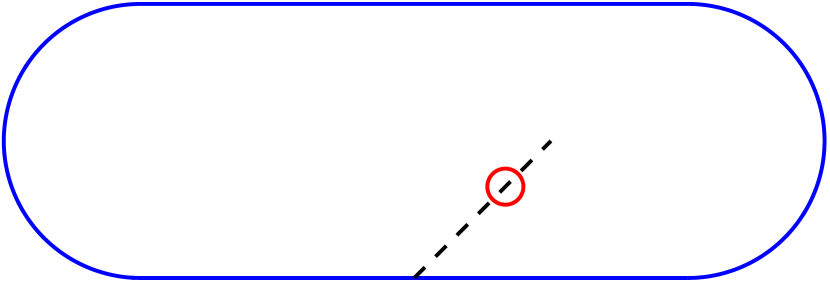
(a) $n_{1}=1$ and $n_{2}=4$, $4312$ triangles.

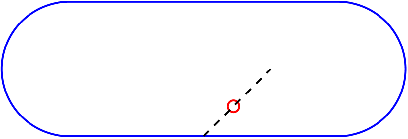
(b) $n_{1}=2$ and $n_{2}=4$, $4364$ triangles.

Figure 2: Different computational domains.

To approximate the solution $u_{{\boldsymbol{\varepsilon}}}$ of the boundary value problem, we use a $\mathbb{P}^{4}$ finite element method on an adapted triangular mesh as provided by the Finite Element Library MÉLINA (see [28]). Figures 3–5 exhibit the computed square root of the energy integral, this is the norm $\|\nabla u_{{\boldsymbol{\varepsilon}}}\|_{{\mathscr{L}}^{2}(\Omega_{{\boldsymbol{\varepsilon}}})}$, in the previously defined configurations. In Figure 3, we take $g^{\mathrm{o}}=0$ and $g^{\mathrm{i}}=1$, so the sum in (1.16) is $0$ and the limiting energy (1.21) is strictly positive (note that with such $g^{o}$ and $g^{i}$ the energy coincides with the electrostatic capacity of $\omega_{{\boldsymbol{\varepsilon}}}$ in $\Omega$).

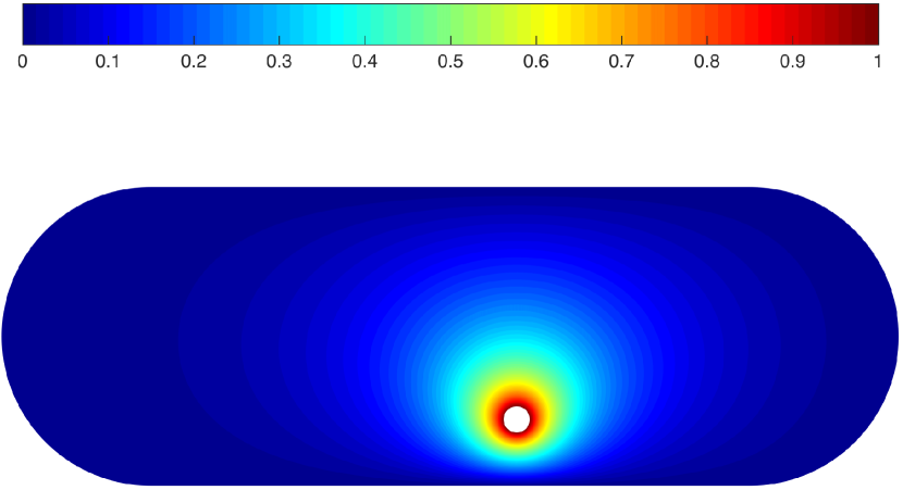
(a) $u_{{\boldsymbol{\varepsilon}}}$ for $n_{1}=2$ and $n_{2}=4$.

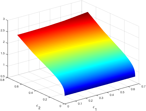
(b) Norm $\|\nabla u_{{\boldsymbol{\varepsilon}}}\|_{{\mathscr{L}}^{2}(\Omega_{{\boldsymbol{\varepsilon}}})}$.

Figure 3: Case where $g^{\mathrm{o}}=0$ and $g^{\mathrm{i}}=1$.

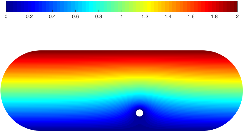
(a) $u_{{\boldsymbol{\varepsilon}}}$ for $n_{1}=2$ and $n_{2}=4$.

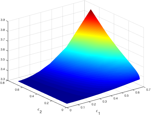
(b) Norm $\|\nabla u_{{\boldsymbol{\varepsilon}}}\|_{{\mathscr{L}}^{2}(\Omega_{{\boldsymbol{\varepsilon}}})}$.

Figure 4: Case $g^{\mathrm{i}}=0$ and $g^{\mathrm{o}}=x_{2}$.

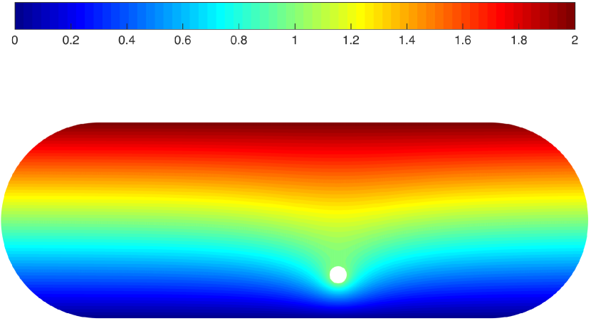
(a) $u_{{\boldsymbol{\varepsilon}}}$ for $n_{1}=2$ and $n_{2}=4$.

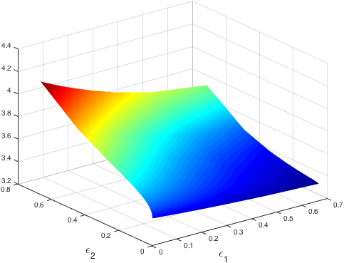
(b) Norm $\|\nabla u_{{\boldsymbol{\varepsilon}}}\|_{{\mathscr{L}}^{2}(\Omega_{{\boldsymbol{\varepsilon}}})}$.

Figure 5: Case $g^{\mathrm{i}}=1$ and $g^{\mathrm{o}}=x_{2}$.

To illustrate the different types of behavior of the energy integral, we now consider $g^{\mathrm{o}}=x_{2}$ and either $g^{\mathrm{i}}=0=g^{\mathrm{o}}(0)$ (see Figure 4), or $g^{\mathrm{i}}=1\neq g^{\mathrm{o}}(0)$ (see Figure 5). Notice that with that choice of $g^{\mathrm{o}}$, we have $\|\nabla u_{0}\|_{{\mathscr{L}}^{2}(\Omega)}=\sqrt{8+\pi}\simeq 3.34$, which is the limiting value observed when $g^{\mathrm{i}}=0$ in Figure 4. On the contrary, in the numerical results for $g^{\mathrm{i}}=1$, the energy has a different limiting value whether both $\varepsilon_{1}$ and $\varepsilon_{2}$ tend to $0$ or $\varepsilon_{1}$ tends to $0$ with $\varepsilon_{2}$ fixed, in agreement with our expectation when $g^{\mathrm{i}}\neq g^{\mathrm{o}}(0)$. When both $\varepsilon_{1}$ and $\varepsilon_{2}$ tend to $0$, the limiting value of the energy is the same as in the well-known case where $\varepsilon_{2}\to 0$ with $\varepsilon_{1}$ fixed (that is, when the hole shrinks to an interior point of $\Omega$). We notice that in the latter case, the energy appears to converge at a slow logarithmic rate (see, in particular, Figures 3 and 5); this is also a well-known fact, predicted by theoretical analysis (see, e.g., Maz’ya, Nazarov, and Plamenevskij [30]).

1.5 Structure of the paper

The paper is organised as follows. In Section 2, we present some preliminary results in potential theory and study the layer potentials with integral kernels consisting of the Dirichlet Green’s function of the half space. Section 3 is devoted to the $n\geq 3$ dimensional case. Here we prove our analyticity result stated in Theorem 1.2. In Section 4, we study the two-dimensional case for ${\boldsymbol{\varepsilon}}\to{\boldsymbol{0}}$. In particular, we prove Theorem 1.3. In Section 5, we consider the case where $n=2$ and $\varepsilon_{1}\to 0$ with $\varepsilon_{2}=1$ fixed and we prove Theorem 1.4. Concluding remarks are presented in Section 6. Some routine technical tools have been placed in the Appendix. Specifically, in A we prove some decay properties of the Green’s function and the associated single-layer potential, and in B we present an extension result based on the Cauchy-Kovalevskaya Theorem.

2 Preliminaries of potential theory

In this section, we introduce some technical results and notation. Most of them deal with the potential theory constructed with the Dirichlet Green’s function of the upper half space. Throughout the section we take

$$n\in\mathbb{N}\setminus\{0,1\}\,.$$

2.1 Classical single and double layer potentials

As a first step, we introduce the classical layer potentials for the Laplace equation and thus we introduce the fundamental solution $S_{n}$ of $\Delta$ defined by

$$S_{n}(\mathsf{x})\equiv\begin{cases}\frac{1}{s_{n}}\log|\mathsf{x}|&\text{if }n=2\,,\\[5.0pt] \frac{1}{(2-n)s_{n}}|\mathsf{x}|^{2-n}&\text{if }n\geq 3\,,\end{cases}\qquad\forall\mathsf{x}\in\mathbb{R}^{n}\setminus\{0\}\,,$$

where $s_{n}$ is the $(n-1)$-dimensional measure of the boundary of the unit ball in $\mathbb{R}^{n}$. In the sequel $\mathcal{D}$ is a generic open bounded connected subset of $\mathbb{R}^{n}$ of class ${\mathscr{C}}^{1,\alpha}$.

Definition 2.1 (Definition of the layer potentials).

For any $\phi\in{\mathscr{C}}^{0,\alpha}(\partial\mathcal{D})$, we define

$$v_{S_{n}}[\partial\mathcal{D},\phi](\mathsf{x})\equiv\int_{\partial\mathcal{D}}\phi(\mathsf{y})S_{n}(\mathsf{x}-\mathsf{y})\,d\sigma_{\mathsf{y}},\qquad\forall\mathsf{x}\in\mathbb{R}^{n}\,,$$

where $d\sigma$ denotes the area element on $\partial\mathcal{D}$.
The restrictions of $v_{S_{n}}[\partial\mathcal{D},\phi]$ to $\overline{\mathcal{D}}$ and to $\mathbb{R}^{n}\setminus\mathcal{D}$ are denoted $v_{S_{n}}^{i}[\partial\mathcal{D},\phi]$ and $v_{S_{n}}^{e}[\partial\mathcal{D},\phi]$ respectively (the letter ‘$i$’ stands for ‘interior’ while the letter ‘$e$’ stands for ‘exterior’).
For any $\psi\in{\mathscr{C}}^{1,\alpha}(\partial\mathcal{D})$, we define

$$w_{S_{n}}[\partial\mathcal{D},\psi](\mathsf{x})\equiv-\int_{\partial\mathcal{D}}\psi(\mathsf{y})\;{\boldsymbol{\mathsf{n}}}_{\mathcal{D}}(\mathsf{y})\cdot\nabla S_{n}(\mathsf{x}-\mathsf{y})\,d\sigma_{\mathsf{y}},\qquad\forall\mathsf{x}\in\mathbb{R}^{n}\,,$$

where ${\boldsymbol{\mathsf{n}}}_{\mathcal{D}}$ denotes the outer unit normal to $\partial\mathcal{D}$ and the symbol $\cdot$ denotes the scalar product in $\mathbb{R}^{n}$.

To describe the regularity properties of these layer potentials we will need the following definition.

Definition 2.2.

We denote by ${\mathscr{C}}^{1,\alpha}_{\mathrm{loc}}(\mathbb{R}^{n}\setminus\mathcal{D})$ the space of functions on $\mathbb{R}^{n}\setminus\mathcal{D}$ whose restrictions to $\overline{\mathcal{O}}$ belong to ${\mathscr{C}}^{1,\alpha}(\overline{\mathcal{O}})$ for all open bounded subsets $\mathcal{O}$ of $\mathbb{R}^{n}\setminus\mathcal{D}$.
${\mathscr{C}}^{0,\alpha}_{\#}(\partial\mathcal{D})$ denotes the subspace of ${\mathscr{C}}^{0,\alpha}(\partial\mathcal{D})$ consisting of the functions $\phi$ with $\int_{\partial\mathcal{D}}\phi\,d\sigma=0$.

Let us now present some well known regularity properties of the single and double layer potentials.

Proposition 2.3 (Regularity of layer potentials).

If $\phi\in{\mathscr{C}}^{0,\alpha}(\partial\mathcal{D})$, then the function $v_{S_{n}}[\partial\mathcal{D},\phi]$ is continuous from $\mathbb{R}^{n}$ to $\mathbb{R}$. Moreover, the restrictions $v_{S_{n}}^{i}[\partial\mathcal{D},\phi]$ and $v_{S_{n}}^{e}[\partial\mathcal{D},\phi]$ belong to ${\mathscr{C}}^{1,\alpha}(\overline{\mathcal{D}})$ and to ${\mathscr{C}}^{1,\alpha}_{\mathrm{loc}}(\mathbb{R}^{n}\setminus\mathcal{D})$, respectively.
If $\psi\in{\mathscr{C}}^{1,\alpha}(\partial\mathcal{D})$, then the restriction $w_{S_{n}}[\partial\mathcal{D},\psi]_{|\mathcal{D}}$ extends to a function $w_{S_{n}}^{i}[\partial\mathcal{D},\psi]$ of ${\mathscr{C}}^{1,\alpha}(\overline{\mathcal{D}})$ and the restriction $w_{S_{n}}[\partial\mathcal{D},\psi]_{|\mathbb{R}^{n}\setminus\overline{\mathcal{D}}}$ extends to a function $w_{S_{n}}^{e}[\partial\mathcal{D},\psi]$ of ${\mathscr{C}}^{1,\alpha}_{\mathrm{loc}}(\mathbb{R}^{n}\setminus\mathcal{D})$.

In the next Proposition 2.4 we recall the classical jump formulas (see, e.g., Folland [18, Chap. 3]).

Proposition 2.4 (Jump relations of layer potentials).

For any $\mathsf{x}\in\partial\mathcal{D}$, $\psi\in{\mathscr{C}}^{1,\alpha}(\partial\mathcal{D})$, and $\phi\in{\mathscr{C}}^{0,\alpha}(\partial\mathcal{D})$, we have

$$w_{S_{n}}^{\sharp}[\partial\mathcal{D},\psi](\mathsf{x}) =\frac{{\mathsf{s}}_{\sharp}}{2}\psi(\mathsf{x})+w_{S_{n}}[\partial\mathcal{D},\psi](\mathsf{x})\,,$$

$${\boldsymbol{\mathsf{n}}}_{\Omega}(\mathsf{x})\cdot\nabla v_{S_{n}}^{\sharp}[\partial\mathcal{D},\phi](\mathsf{x}) =-\frac{{\mathsf{s}}_{\sharp}}{2}\phi(\mathsf{x})+\int_{\partial\mathcal{D}}\phi(\mathsf{y}){\boldsymbol{\mathsf{n}}}_{\Omega}(\mathsf{x})\cdot\nabla S_{n}(\mathsf{x}-\mathsf{y})\,d\sigma_{\mathsf{y}}\,,$$

where $\sharp=i,e$ and ${\mathsf{s}}_{i}=1$, ${\mathsf{s}}_{e}=-1$.

We will exploit the following classical result of potential theory.

Lemma 2.5.

The map $\begin{array}[]{rcl}&\\ {\mathscr{C}}^{0,\alpha}_{\#}(\partial\mathcal{D})\times\mathbb{R}&\to&{\mathscr{C}}^{1,\alpha}(\partial\mathcal{D})\\ (\phi,\xi)&\mapsto&v_{S_{n}}[\partial\mathcal{D},\phi]_{|\partial\mathcal{D}}+\xi\end{array}$ is an isomorphism.
Moreover, if $n\geq 3$, then the map $\begin{array}[]{rcl}&\\ {\mathscr{C}}^{0,\alpha}(\partial\mathcal{D})&\to&{\mathscr{C}}^{1,\alpha}(\partial\mathcal{D})\\ \phi&\mapsto&v_{S_{n}}[\partial\mathcal{D},\phi]_{|\partial\mathcal{D}}\end{array}$ is an isomorphism.

2.2 Green’s function for the upper half space and associated layer potentials

As mentioned above, a key tool for the analysis of problem (1.2) are layer potentials constructed with the Dirichlet Green’s function of the upper half space instead of the classical fundamental solution $S_{n}$. Transforming problem (1.2) by means of these layer potentials will lead us to a system of integral equations with no integral equation on $\partial_{0}\Omega$, which is the part of the boundary of $\partial\Omega$ where the inclusion $\omega_{{\boldsymbol{\varepsilon}}}$ collapses for ${\boldsymbol{\varepsilon}}=\bf 0$.

Let us begin by introducing some notation. We denote by $\mathsf{\varsigma}$ the reflexion with respect to the hyperplane $\partial\mathbb{R}^{n}_{+}$, so that

$$\mathsf{\varsigma}(\mathsf{x})\equiv(x_{1},\dots,x_{n-1},-x_{n})\,,\qquad\forall\mathsf{x}=(x_{1},\dots,x_{n})\in\mathbb{R}^{n}\,.$$

Then we denote by ${{G}}$ the Green’s function defined by

$${{G}}(\mathsf{x},\mathsf{y})\equiv S_{n}(\mathsf{x}-\mathsf{y})-S_{n}(\mathsf{\varsigma}(\mathsf{x})-\mathsf{y}),\quad\forall(\mathsf{x},\mathsf{y})\in\mathbb{R}^{n}\times\mathbb{R}^{n}\text{ with }\mathsf{y}\neq\mathsf{x}\text{ and }\mathsf{y}\neq\mathsf{\varsigma}(\mathsf{x}).$$

We observe that

$${{G}}(\mathsf{x},\mathsf{y})={{G}}(\mathsf{y},\mathsf{x}),\quad\forall(\mathsf{x},\mathsf{y})\in\mathbb{R}^{n}\times\mathbb{R}^{n}\text{ with }\mathsf{y}\neq\mathsf{x}\text{ and }\mathsf{y}\neq\mathsf{\varsigma}(\mathsf{x}),$$ (2.1)

and

$${{G}}(\mathsf{x},\mathsf{y})=0,\quad\forall(\mathsf{x},\mathsf{y})\in\partial\mathbb{R}^{n}_{+}\times\mathbb{R}^{n}\text{ with }\mathsf{y}\neq\mathsf{x}\text{ and }\mathsf{y}\neq\mathsf{\varsigma}(\mathsf{x}).$$ (2.2)

We denote by the symbols $\nabla_{\mathsf{x}}{{G}}(\mathsf{x},\mathsf{y})$ and $\nabla_{\mathsf{y}}{{G}}(\mathsf{x},\mathsf{y})$ the gradient of the function $\mathsf{x}\mapsto{{G}}(\mathsf{x},\mathsf{y})$ and of the function $\mathsf{y}\mapsto{{G}}(\mathsf{x},\mathsf{y})$, respectively. If $\mathcal{D}$ is a subset of $\mathbb{R}^{n}$, we find convenient to set $\mathsf{\varsigma}(\mathcal{D})\equiv\{\mathsf{x}\in\mathbb{R}^{n}\;|\;\mathsf{\varsigma}(\mathsf{x})\in\mathcal{D}\}$. We now introduce analogs of the classical layer potentials of Definition 2.2 obtained by replacing $S_{n}$ by the Green’s function ${{G}}$. In the sequel, $\mathcal{D}_{+}$ denotes an open bounded connected set contained in $\mathbb{R}^{n}_{+}$ and of class ${\mathscr{C}}^{1,\alpha}$.

Definition 2.6 (Definition of layer potentials derived by $G$).

For any $\phi\in{\mathscr{C}}^{0,\alpha}(\partial\mathcal{D}_{+})$, we define

$$v_{{{G}}}[\partial\mathcal{D}_{+},\phi](\mathsf{x})\equiv\int_{\partial\mathcal{D}_{+}}\phi(\mathsf{y}){{G}}(\mathsf{x},\mathsf{y})\,d\sigma_{\mathsf{y}},\qquad\forall\mathsf{x}\in\mathbb{R}^{n}\,.$$

The restrictions of $v_{{{G}}}[\partial\mathcal{D}_{+},\phi]$ to $\overline{\mathcal{D}}_{+}$ and $\overline{\mathbb{R}^{n}_{+}\setminus\mathcal{D}_{+}}$ are denoted $v_{{{G}}}^{i}[\partial\mathcal{D}_{+},\phi]$ and $v_{{{G}}}^{e}[\partial\mathcal{D}_{+},\phi]$ respectively.
For any subset $\Gamma$ of the boundary $\partial\mathcal{D}_{+}$ and for any $\psi\in{\mathscr{C}}^{1,\alpha}(\partial\mathcal{D}_{+})$, we define

$$w_{{{G}}}[\Gamma,\psi](\mathsf{x})\equiv\int_{\Gamma}\psi(\mathsf{y})\;{\boldsymbol{\mathsf{n}}}_{\mathcal{D}_{+}}(\mathsf{y})\cdot\nabla_{\mathsf{y}}\,{{G}}(\mathsf{x},\mathsf{y})\,d\sigma_{\mathsf{y}},\qquad\forall\mathsf{x}\in\mathbb{R}^{n}\,.$$

By the definition of ${{G}}$, we easily obtain the equalities

$$v_{{{G}}}[\partial\mathcal{D}_{+},\phi](\mathsf{x})=v_{S_{n}}[\partial\mathcal{D}_{+},\phi](\mathsf{x})-v_{S_{n}}[\partial\mathcal{D}_{+},\phi](\mathsf{\varsigma}(\mathsf{x}))\,,\qquad\forall\mathsf{x}\in\mathbb{R}^{n}\\ ,\ \forall\phi\in{\mathscr{C}}^{0,\alpha}(\partial\mathcal{D}_{+})\,,$$

and

$$w_{{{G}}}[\partial\mathcal{D}_{+},\psi](\mathsf{x})=w_{S_{n}}[\partial\mathcal{D}_{+},\psi](\mathsf{x})-w_{S_{n}}[\partial\mathcal{D}_{+},\psi](\mathsf{\varsigma}({\mathsf{x}}))\,,\qquad\forall\mathsf{x}\in\mathbb{R}^{n}\,,\ \forall\psi\in{\mathscr{C}}^{1,\alpha}(\partial\mathcal{D}_{+})\,.$$

Thus one deduces by Propositions 2.3 and 2.4 the regularity properties and jump formulas for $v_{{{G}}}[\partial\mathcal{D}_{+},\phi]$ and $w_{{{G}}}[\partial\mathcal{D}_{+},\psi]$.

Proposition 2.7 (Regularity and jump relations for the layer potentials derived by $G$).

Let $\phi\in{\mathscr{C}}^{0,\alpha}(\partial\mathcal{D}_{+})$ and $\psi\in{\mathscr{C}}^{1,\alpha}(\partial\mathcal{D}_{+})$. Then

• the functions $v_{{{G}}}[\partial\mathcal{D}_{+},\phi]$ and $w_{{{G}}}[\partial\mathcal{D}_{+},\psi]$ are harmonic in $\mathcal{D}_{+}$, $\mathsf{\varsigma}({\mathcal{D}_{+}})$, and $\mathbb{R}^{n}\setminus\overline{\mathcal{D}_{+}\cup\mathsf{\varsigma}({\mathcal{D}_{+}})}$;

• the function $v_{{{G}}}[\partial\mathcal{D}_{+},\phi]$ is continuous from $\mathbb{R}^{n}$ to $\mathbb{R}$ and the restrictions $v_{{{G}}}^{i}[\partial\mathcal{D}_{+},\phi]$ and $v_{{{G}}}^{e}[\partial\mathcal{D}_{+},\phi]$ belong to ${\mathscr{C}}^{1,\alpha}(\overline{\mathcal{D}_{+}})$ and to ${\mathscr{C}}^{1,\alpha}_{\mathrm{loc}}(\overline{\mathbb{R}^{n}_{+}\setminus\mathcal{D}_{+}})$, respectively;

• the restriction $w_{{{G}}}[\partial\mathcal{D}_{+},\psi]_{|\Omega}$ extends to a function $w_{{{G}}}^{i}[\partial\mathcal{D}_{+},\psi]$ of ${\mathscr{C}}^{1,\alpha}(\overline{\mathcal{D}_{+}})$ and the restriction $w_{{{G}}}[\partial\mathcal{D}_{+},\psi]_{|\mathbb{R}^{n}_{+}\setminus\overline{\mathcal{D}_{+}}}$ extends to a function $w_{{{G}}}^{e}[\partial\mathcal{D}_{+},\psi]$ of ${\mathscr{C}}^{1,\alpha}_{\mathrm{loc}}(\overline{\mathbb{R}^{n}_{+}\setminus\mathcal{D}_{+}})$.

The jump formulas for the double layer potential are (with $\sharp=i,e$, ${\mathsf{s}}_{i}=1$, ${\mathsf{s}}_{e}=-1$)

$$w_{{{G}}}^{\sharp}[\partial\mathcal{D}_{+},\psi](\mathsf{x}) =\frac{{\mathsf{s}}_{\sharp}}{2}\psi(\mathsf{x})+w_{{{G}}}[\partial\mathcal{D}_{+},\psi](\mathsf{x}), \forall\mathsf{x}\in\partial_{+}\mathcal{D}_{+}\,,$$

$$w_{{{G}}}^{i}[\partial\mathcal{D}_{+},\psi](\mathsf{x}) =\psi(\mathsf{x}), \forall\mathsf{x}\in\partial_{0}\mathcal{D}_{+}\,.$$

Moreover, we have

$$v_{{{G}}}[\partial\mathcal{D}_{+},\phi](\mathsf{x})=0, \qquad\forall\mathsf{x}\in\partial\mathbb{R}^{n}_{+}\,,$$ (2.3)

$$w^{e}_{{{G}}}[\partial\mathcal{D}_{+},\psi](\mathsf{x})=0, \qquad\forall\mathsf{x}\in\partial\mathbb{R}^{n}_{+}\setminus\partial_{0}\mathcal{D}_{+}\,.$$

Here above, $\partial_{0}\mathcal{D}_{+}\equiv\partial\mathcal{D}_{+}\cap\partial\mathbb{R}^{n}_{+}$ and $\partial_{+}\mathcal{D}_{+}\equiv\partial\mathcal{D}_{+}\cap\mathbb{R}^{n}_{+}$.

In the following lemma we show how the layer potentials with kernel $G$ introduced in Definition 2.6 allow to prove a corresponding Green-like representation formula.

Lemma 2.8 (Green-like representation formula in $\mathcal{D}_{+}$).

Let $u^{i}\in{\mathscr{C}}^{1,\alpha}(\overline{\mathcal{D}_{+}})$ be such that $\Delta u^{i}=0$ in $\mathcal{D}_{+}$. Then we have

$$w_{{{G}}}[\partial\mathcal{D}_{+},u^{i}_{|\partial\mathcal{D}_{+}}]-v_{{{G}}}[\partial\mathcal{D}_{+},{\boldsymbol{\mathsf{n}}}_{\mathcal{D}_{+}}\cdot\nabla u^{i}_{|\partial\mathcal{D}_{+}}]=\begin{cases}u^{i}&\mbox{ in }\mathcal{D}_{+},\\ 0&\mbox{ in }\mathbb{R}^{n}\setminus\overline{\mathcal{D}_{+}\cup\mathsf{\varsigma}(\mathcal{D}_{+})}\,.\end{cases}$$ (2.4)

• Proof. Let us first consider $\mathsf{x}\in\mathcal{D}_{+}$. By the Green’s representation formula (see, e.g., Folland [18, Chap. 2]), we have

  $$u^{i}(\mathsf{x})=-\int_{\partial\mathcal{D}_{+}}{\boldsymbol{\mathsf{n}}}_{\mathcal{D}_{+}}(\mathsf{y})\cdot\nabla S_{n}(\mathsf{x}-\mathsf{y})\,u^{i}(\mathsf{y})\,d\sigma_{\mathsf{y}}-\int_{\partial\mathcal{D}_{+}}S_{n}(\mathsf{x}-\mathsf{y})\;{\boldsymbol{\mathsf{n}}}_{\mathcal{D}_{+}}(\mathsf{y})\cdot\nabla u^{i}(\mathsf{y})\,d\sigma_{\mathsf{y}}{\color[rgb]{0,0,1},\quad}\forall\mathsf{x}\in\mathcal{D}_{+}\,.$$ (2.5)

  On the other hand, we note that if $\mathsf{x}\in\mathcal{D}_{+}$ is fixed, then the function $\mathsf{y}\mapsto S_{n}(\mathsf{\varsigma}({\mathsf{x}})-\mathsf{y})$ is of class ${\mathscr{C}}^{1}(\overline{\mathcal{D}_{+}})$ and harmonic in $\mathcal{D}_{+}$. Therefore, by the Green’s identity, we have

  $$0=\int_{\partial\mathcal{D}_{+}}{\boldsymbol{\mathsf{n}}}_{\mathcal{D}_{+}}(\mathsf{y})\cdot\nabla S_{n}(\mathsf{\varsigma}({\mathsf{x}})-\mathsf{y})\,u^{i}(\mathsf{y})\,d\sigma_{\mathsf{y}}+\int_{\partial\mathcal{D}_{+}}S_{n}(\mathsf{\varsigma}({\mathsf{x}})-\mathsf{y})\;{\boldsymbol{\mathsf{n}}}_{\mathcal{D}_{+}}(\mathsf{y})\cdot\nabla u^{i}(\mathsf{y})\,d\sigma_{\mathsf{y}}\qquad\forall\mathsf{x}\in\mathcal{D}_{+}\,.$$ (2.6)

  Then, by summing equalities (2.5) and (2.6) we deduce the validity of (2.4) in $\mathcal{D}_{+}$.
  Let us now consider any fixed $\mathsf{x}\in\mathbb{R}^{n}\setminus\overline{\mathcal{D}_{+}\cup\mathsf{\varsigma}(\mathcal{D}_{+})}$. We observe that the functions $\mathsf{y}\mapsto S_{n}(\mathsf{x}-\mathsf{y})$ and $\mathsf{y}\mapsto S_{n}(\mathsf{\varsigma}(\mathsf{x})-\mathsf{y})$ are harmonic on $\mathcal{D}_{+}$. Accordingly ${{G}}(\mathsf{x},\cdot)$ is an harmonic function in $\mathcal{D}_{+}$. Then a standard argument based on the divergence theorem shows that

  $$\int_{\partial\mathcal{D}_{+}}u^{i}(\mathsf{y})\;{\boldsymbol{\mathsf{n}}}_{\mathcal{D}_{+}}(\mathsf{y})\cdot\nabla_{\mathsf{y}}{{G}}(\mathsf{x},\mathsf{y})-{{G}}(\mathsf{x},\mathsf{y})\;{\boldsymbol{\mathsf{n}}}_{\mathcal{D}_{+}}(\mathsf{y})\cdot\nabla u^{i}(\mathsf{y})\;d\sigma_{\mathsf{y}}=0\,.$$

  $\blacksquare$

2.3 Mapping properties of the single layer potential $v_{{{G}}}[\partial\Omega,\cdot]$

In order to analyze the ${\boldsymbol{\varepsilon}}$-dependent boundary value problem (1.2), we are going to exploit the layer potentials with kernel derived by $G$ in the case when $\mathcal{D}=\Omega_{{\boldsymbol{\varepsilon}}}$. Since $\partial\Omega_{{\boldsymbol{\varepsilon}}}=\partial\Omega\cup\partial\omega_{{\boldsymbol{\varepsilon}}}$, we need to consider layer potentials integrated on $\partial\Omega$ and on $\partial\omega_{{\boldsymbol{\varepsilon}}}$. In this section, we will investigate some properties of the single layer potential supported on the boundary of the set $\Omega$ which satisfies the assumptions ($H_{1}$), ($H_{2}$), and ($H_{3}$).

First of all, as one can easily see, the single layer potential $v_{{{G}}}[\partial\Omega,\phi]$ does not depend on the values of the density $\phi$ on $\partial_{0}\Omega$. In other words, it takes into account only $\phi_{|\partial_{+}\Omega}$. For this reason, it is convenient to introduce a quotient Banach space.

Definition 2.9.

We denote by ${\mathscr{C}}^{0,\alpha}_{+}(\partial\Omega)$ the quotient Banach space

$${\mathscr{C}}^{0,\alpha}(\partial\Omega)/\{\phi\in{\mathscr{C}}^{0,\alpha}(\partial\Omega)\;|\;\phi_{|\partial_{+}\Omega}=0\}\,.$$

Then we can prove that the single layer potential map

$$\begin{array}[]{rcl}{\mathscr{C}}^{0,\alpha}_{+}(\partial\Omega)&\to&{\mathscr{C}}^{1,\alpha}(\partial_{+}\Omega)\\ \phi&\mapsto&v_{{{G}}}[\partial\Omega,\phi]_{|\partial_{+}\Omega}\end{array}$$

is well defined and one-to-one. Namely we have the following.

Proposition 2.10 (Null space of the single layer potential derived by $G$).

Let $\phi\in{\mathscr{C}}^{0,\alpha}(\partial\Omega)$. Then $v_{{{G}}}[\partial\Omega,\phi]_{|\partial_{+}\Omega}=0$ if and only if $\phi_{|\partial_{+}\Omega}=0$.

• Proof. Let $\phi\in{\mathscr{C}}^{0,\alpha}(\partial\Omega)$ be such that $\phi_{|\partial_{+}\Omega}=0$. As a consequence,

  $$v_{{{G}}}[\partial\Omega,\phi](\mathsf{x})=\int_{\partial_{+}\Omega}{{G}}(\mathsf{x},\mathsf{y})\phi_{|\partial_{+}\Omega}(\mathsf{y})\,d\sigma_{\mathsf{y}}=0\qquad\forall\mathsf{x}\in\partial\Omega\,.$$

  Let now assume that $v_{{{G}}}[\partial\Omega,\phi]_{|\partial_{+}\Omega}=0$. With (2.3), we have in particular $v_{{{G}}}[\partial\Omega,\phi]_{|\partial_{0}\Omega}=0$ and then $v_{{{G}}}[\partial\Omega,\phi]_{|\partial\Omega}=0$. By the uniqueness of the solution of the Dirichlet problem we deduce that $v_{{{G}}}[\partial\Omega,\phi]=0$ in $\overline{\Omega}$. By the harmonicity at infinity of $v_{{{G}}}[\partial\Omega,\phi]$ (cf. Lemma A.2), by equality $v_{{{G}}}[\partial\Omega,\phi]_{|\partial\mathbb{R}^{n}_{+}\cup\partial\Omega}=0$, and by a standard energy argument based on the divergence theorem, we deduce that $\nabla v_{{{G}}}[\partial\Omega,\phi]=0$ in $\mathbb{R}^{n}_{+}\setminus\overline{\Omega}$, and that accordingly $v_{{{G}}}[\partial\Omega,\phi]$ is constant in $\mathbb{R}^{n}_{+}\setminus\Omega$. Since $v_{{{G}}}[\partial\Omega,\phi]=0$ on $\partial\Omega$, we have $v_{{{G}}}[\partial\Omega,\phi]=0$ in $\mathbb{R}^{n}_{+}$. Then, for the normal derivative of $v_{{{G}}}[\partial\Omega,\phi]$ on $\partial_{+}\Omega$ we have the following jump formulas:

  $${\boldsymbol{\mathsf{n}}}_{\Omega}(\mathsf{x})\cdot\nabla v_{{{G}}}^{\sharp}[\partial\Omega,\phi](\mathsf{x})=-\frac{{\mathsf{s}}_{\sharp}}{2}\phi(\mathsf{x})+\int_{\partial_{+}\Omega}\phi(\mathsf{y}){\boldsymbol{\mathsf{n}}}_{\Omega}(\mathsf{x})\cdot\nabla_{\mathsf{x}}{{G}}(\mathsf{x},\mathsf{y})\,d\sigma_{\mathsf{y}},\qquad\forall\mathsf{x}\in\partial_{+}\Omega\,,$$

  with $\sharp=i,e$, ${\mathsf{s}}_{i}=1$, ${\mathsf{s}}_{e}=-1$. It follows that

  $$\phi={\boldsymbol{\mathsf{n}}}_{\Omega}\cdot\nabla v^{e}_{{{G}}}[\partial\Omega,\phi]-{\boldsymbol{\mathsf{n}}}_{\Omega}\cdot\nabla v^{i}_{{{G}}}[\partial\Omega,\phi]=0\qquad\text{on $\partial_{+}\Omega$}\,,$$

  and thus the proof is complete. $\blacksquare$

By the previous Proposition 2.10 one readily verifies the validity of the following Proposition 2.11 where we introduce the image space ${\mathscr{V}}^{1,\alpha}(\partial_{+}\Omega)$ of $v_{{{G}}}[\partial\Omega,\cdot]_{|\partial_{+}\Omega}$.

Proposition 2.11 (Image of the single layer potential derived by $G$).

Let ${\mathscr{V}}^{1,\alpha}(\partial_{+}\Omega)$ denote the vector space

$${\mathscr{V}}^{1,\alpha}(\partial_{+}\Omega)=\left\{v_{{{G}}}[\partial\Omega,\phi]_{|\partial_{+}\Omega},\ \forall\phi\in{\mathscr{C}}^{0,\alpha}_{+}(\partial\Omega)\right\}.$$

Let $\|\cdot\|_{{\mathscr{V}}^{1,\alpha}(\partial_{+}\Omega)}$ be the norm on ${\mathscr{V}}^{1,\alpha}(\partial_{+}\Omega)$ defined by

$$\|f\|_{{\mathscr{V}}^{1,\alpha}(\partial_{+}\Omega)}\equiv\|\phi\|_{{\mathscr{C}}^{0,\alpha}_{+}(\partial\Omega)}$$

for all $(f,\phi)\in{\mathscr{V}}^{1,\alpha}(\partial_{+}\Omega)\times{\mathscr{C}}^{0,\alpha}_{+}(\partial\Omega)$ such that $f=v_{{{G}}}[\partial\Omega,\phi]_{|\partial_{+}\Omega}$. Then the following statements hold.

1. ${\mathscr{V}}^{1,\alpha}(\partial_{+}\Omega)$ endowed with the norm $\|\cdot\|_{{\mathscr{V}}^{1,\alpha}(\partial_{+}\Omega)}$ is a Banach space.

2. The operator $v_{{{G}}}[\partial\Omega,\cdot]_{|\partial\Omega}$ is an homeomorphism from ${\mathscr{C}}^{0,\alpha}_{+}(\partial\Omega)$ to ${\mathscr{V}}^{1,\alpha}(\partial_{+}\Omega)$.

2.3.1 Characterization of the image of the single layer potential

We wish now to characterize the functions of ${\mathscr{V}}^{1,\alpha}(\partial_{+}\Omega)$, that is the set of the elements of ${\mathscr{C}}^{1,\alpha}(\partial\Omega)$ that can be represented as $v_{{{G}}}[\partial\Omega,\phi]_{|\partial_{+}\Omega}$ for some $\phi\in{\mathscr{C}}^{0,\alpha}_{+}(\partial\Omega)$. We do so in the following Proposition 2.12.

Proposition 2.12.

Let $f\in{\mathscr{C}}^{1,\alpha}(\partial_{+}\Omega)$. Then $f$ belongs to ${\mathscr{V}}^{1,\alpha}(\partial_{+}\Omega)$ if and only if $f=u^{e}_{|\partial_{+}\Omega}$, where $u^{e}$ is a function of ${\mathscr{C}}^{1,\alpha}_{\mathrm{loc}}(\overline{\mathbb{R}^{n}_{+}\setminus\Omega})$ such that

$$\begin{cases}\Delta u^{e}=0\quad\mbox{ in }\mathbb{R}^{n}_{+}\setminus\overline{\Omega},\\ u^{e}=0\quad\mbox{ on }\partial\mathbb{R}^{n}_{+}\setminus\partial_{0}\Omega,\\ \lim_{\mathsf{x}\to\infty}\frac{1}{|\mathsf{x}|}u^{e}(\mathsf{x})=0,\\ \lim_{\mathsf{x}\to\infty}\frac{\mathsf{x}}{|\mathsf{x}|}\cdot\nabla u^{e}(\mathsf{x})=0.\end{cases}$$ (2.7)

• Proof of Proposition 2.12. We divide the proof in three steps.

$\bullet$ First step: Green-like representation formulas in $\mathbb{R}^{n}_{+}\setminus\overline{\Omega}$. As a first step, we prove a representation formula for harmonic functions in the set $\mathbb{R}^{n}_{+}\setminus\overline{\Omega}$.

Lemma 2.13.

Let $u^{e}\in{\mathscr{C}}^{1,\alpha}_{\mathrm{loc}}(\overline{\mathbb{R}^{n}_{+}\setminus\Omega})$ be such that

$$\begin{cases}\Delta u^{e}=0\quad\mbox{ in }\mathbb{R}^{n}_{+}\setminus\overline{\Omega},\\ \lim_{|\mathsf{x}|\to\infty}\frac{1}{|\mathsf{x}|}u^{e}(\mathsf{x})=0,\\ \lim_{|\mathsf{x}|\to\infty}\frac{\mathsf{x}}{|\mathsf{x}|}\cdot\nabla u^{e}(\mathsf{x})=0.\end{cases}$$

Then we have

$$-w_{{{G}}}[\partial_{+}\Omega,u^{e}_{|\partial_{+}\Omega}](\mathsf{x})+v_{{{G}}}[\partial\Omega,{\boldsymbol{\mathsf{n}}}_{\Omega}\cdot\nabla u^{e}_{|\partial\Omega}](\mathsf{x})+\frac{2x_{n}}{s_{n}}\int_{\partial\mathbb{R}^{n}_{+}\setminus\partial_{0}\Omega}\frac{u^{e}(\mathsf{y})}{|\mathsf{x}-\mathsf{y}|^{n}}\,d\sigma_{\mathsf{y}}\\ =\begin{cases}u^{e}(\mathsf{x})&\forall\mathsf{x}\in\mathbb{R}^{n}_{+}\setminus\overline{\Omega},\\ 0&\forall\mathsf{x}\in\Omega.\end{cases}$$

• Proof. Let $R>\max_{\mathsf{x}\in\overline{\Omega}}|\mathsf{x}|$. Let $\Omega^{e,+}_{R}\equiv\mathbb{R}^{n}_{+}\cap\mathcal{B}(0,R)\setminus\overline{\Omega}$. Let $\mathsf{x}\in\Omega^{e,+}_{R}$. Let $r>0$ and $\mathcal{B}(\mathsf{x},r)\subseteq\Omega^{e,+}_{R}$. By Lemma 2.8 we have

  $$\begin{split}u^{e}(\mathsf{x})&=w_{{{G}}}[\partial\mathcal{B}(\mathsf{x},r),u^{e}_{|\partial\mathcal{B}(\mathsf{x},r)}](\mathsf{x})-v_{{{G}}}[\partial\mathcal{B}(\mathsf{x},r),{\boldsymbol{\mathsf{n}}}_{\mathcal{B}(\mathsf{x},r)}\cdot\nabla u^{e}_{|\partial\mathcal{B}(\mathsf{x},r)}](\mathsf{x})\\ &=\int_{\partial\mathcal{B}(\mathsf{x},r)}u^{e}(\mathsf{y})\;{\boldsymbol{\mathsf{n}}}_{\mathcal{B}(\mathsf{x},r)}(\mathsf{y})\cdot\nabla_{\mathsf{y}}{{G}}(\mathsf{x},\mathsf{y})-{{G}}(\mathsf{x},\mathsf{y})\;{\boldsymbol{\mathsf{n}}}_{\mathcal{B}(\mathsf{x},r)}(\mathsf{y})\cdot\nabla u^{e}(\mathsf{y})\;d\sigma_{\mathsf{y}}\,.\end{split}$$ (2.8)

  Then we observe that ${{G}}(\mathsf{x},\cdot)$ is a harmonic function in $\Omega^{e,+}_{R}\setminus\overline{\mathcal{B}(\mathsf{x},r)}$ and thus by the divergence theorem we have

  $$\begin{split}0&=\int_{\Omega^{e,+}_{R}\setminus\overline{\mathcal{B}(\mathsf{x},r)}}u^{e}(\mathsf{y})\Delta_{\mathsf{y}}{{G}}(\mathsf{x},\mathsf{y})-{{G}}(\mathsf{x},\mathsf{y})\Delta u^{e}(\mathsf{y})\,d\mathsf{x}\\ &=-\int_{\partial\mathcal{B}(\mathsf{x},r)}u^{e}(\mathsf{y})\;{\boldsymbol{\mathsf{n}}}_{\mathcal{B}(\mathsf{x},r)}(\mathsf{y})\cdot\nabla_{\mathsf{y}}{{G}}(\mathsf{x},\mathsf{y})-{{G}}(\mathsf{x},\mathsf{y})\;{\boldsymbol{\mathsf{n}}}_{\mathcal{B}(\mathsf{x},r)}(\mathsf{y})\cdot\nabla u^{e}(\mathsf{y})\;d\sigma_{\mathsf{y}}\\ &\quad+\int_{\partial\Omega^{e,+}_{R}}u^{e}(\mathsf{y})\;{\boldsymbol{\mathsf{n}}}_{\Omega^{e,+}_{R}}(\mathsf{y})\cdot\nabla_{\mathsf{y}}{{G}}(\mathsf{x},\mathsf{y})-{{G}}(\mathsf{x},\mathsf{y})\;{\boldsymbol{\mathsf{n}}}_{\Omega^{e,+}_{R}}(\mathsf{y})\cdot\nabla u^{e}(\mathsf{y})\;d\sigma_{\mathsf{y}}\\ &=-\int_{\partial\mathcal{B}(\mathsf{x},r)}u^{e}(\mathsf{y})\;{\boldsymbol{\mathsf{n}}}_{\mathcal{B}(\mathsf{x},r)}(\mathsf{y})\cdot\nabla_{\mathsf{y}}{{G}}(\mathsf{x},\mathsf{y})-{{G}}(\mathsf{x},\mathsf{y})\;{\boldsymbol{\mathsf{n}}}_{\mathcal{B}(\mathsf{x},r)}(\mathsf{y})\cdot\nabla u^{e}(\mathsf{y})\;d\sigma_{\mathsf{y}}\\ &\quad-\int_{\partial_{+}\Omega}u^{e}(\mathsf{y})\;{\boldsymbol{\mathsf{n}}}_{\Omega}(\mathsf{y})\cdot\nabla_{\mathsf{y}}{{G}}(\mathsf{x},\mathsf{y})-{{G}}(\mathsf{x},\mathsf{y})\;{\boldsymbol{\mathsf{n}}}_{\Omega}(\mathsf{y})\cdot\nabla u^{e}(\mathsf{y})\;d\sigma_{\mathsf{y}}\\ &\quad+\int_{\partial_{+}\mathcal{B}(0,R)}u^{e}(\mathsf{y})\;{\boldsymbol{\mathsf{n}}}_{\mathcal{B}(0,R)}(\mathsf{y})\cdot\nabla_{\mathsf{y}}{{G}}(\mathsf{x},\mathsf{y})-{{G}}(\mathsf{x},\mathsf{y})\;{\boldsymbol{\mathsf{n}}}_{\mathcal{B}(0,R)}(\mathsf{y})\cdot\nabla u^{e}(\mathsf{y})\;d\sigma_{\mathsf{y}}\\ &\quad-\int_{\partial\mathbb{R}^{n}_{+}\cap\mathcal{B}(0,R)\setminus\partial_{0}\Omega}u^{e}(\mathsf{y})\;\partial_{y_{n}}{{G}}(\mathsf{x},\mathsf{y})-{{G}}(\mathsf{x},\mathsf{y})\;\partial_{y_{n}}u^{e}(\mathsf{y})\;d\sigma_{\mathsf{y}}.\end{split}$$

  Using Definition 2.6 and the fact that ${{G}}(\mathsf{x},\mathsf{y})=0$ and $\partial_{y_{n}}{{G}}(\mathsf{x},\mathsf{y})=-2x_{n}s_{n}^{-1}|\mathsf{x}-\mathsf{y}|^{-n}$ for all $\mathsf{y}\in\partial\mathbb{R}^{n}_{+}$, we deduce

  $$\begin{split}0&=-\int_{\partial\mathcal{B}(\mathsf{x},r)}u^{e}(\mathsf{y})\;{\boldsymbol{\mathsf{n}}}_{\mathcal{B}(\mathsf{x},r)}(\mathsf{y})\cdot\nabla_{\mathsf{y}}{{G}}(\mathsf{x},\mathsf{y})-{{G}}(\mathsf{x},\mathsf{y})\;{\boldsymbol{\mathsf{n}}}_{\mathcal{B}(\mathsf{x},r)}(\mathsf{y})\cdot\nabla u^{e}(\mathsf{y})\;d\sigma_{\mathsf{y}}\\ &\quad-w_{{{G}}}[\partial_{+}\Omega,u^{e}_{|\partial_{+}\Omega}](\mathsf{x})+v_{{{G}}}[\partial_{+}\Omega,{\boldsymbol{\mathsf{n}}}_{\Omega}\cdot\nabla u^{e}_{|\partial_{+}\Omega}](\mathsf{x})\\ &\quad+\int_{\partial_{+}\mathcal{B}(0,R)}u^{e}(\mathsf{y})\;{\boldsymbol{\mathsf{n}}}_{\mathcal{B}(0,R)}(\mathsf{y})\cdot\nabla_{\mathsf{y}}{{G}}(\mathsf{x},\mathsf{y})-{{G}}(\mathsf{x},\mathsf{y})\;{\boldsymbol{\mathsf{n}}}_{\mathcal{B}(0,R)}(\mathsf{y})\cdot\nabla u^{e}(\mathsf{y})\;d\sigma_{\mathsf{y}}\\ &\quad+\frac{2x_{n}}{s_{n}}\int_{\partial\mathbb{R}^{n}_{+}\cap\mathcal{B}(0,R)\setminus\partial_{0}\Omega}\frac{u^{e}(\mathsf{y})}{|\mathsf{x}-\mathsf{y}|^{n}}\,d\sigma_{\mathsf{y}}.\end{split}$$

  Then we observe that the maps $\mathsf{y}\mapsto|\mathsf{y}|^{n-1}{{G}}(\mathsf{x},\mathsf{y})$ and $\mathsf{y}\mapsto|\mathsf{y}|^{n}\nabla_{\mathsf{y}}{{G}}(\mathsf{x},\mathsf{y})$ are bounded at infinity (see Lemma A.1). Thus, by taking the limit as $R\to\infty$ we obtain

  $$\begin{split}0&=-\int_{\partial\mathcal{B}(x,r)}u^{e}(\mathsf{y})\;{\boldsymbol{\mathsf{n}}}_{\mathcal{B}(\mathsf{x},r)}(\mathsf{y})\cdot\nabla_{\mathsf{y}}{{G}}(\mathsf{x},\mathsf{y})-{{G}}(\mathsf{x},\mathsf{y})\;{\boldsymbol{\mathsf{n}}}_{\mathcal{B}(\mathsf{x},r)}(\mathsf{y})\cdot\nabla u^{e}(\mathsf{y})\;d\sigma_{\mathsf{y}}\\ &\quad-w_{{{G}}}[\partial_{+}\Omega,u^{e}_{|\partial_{+}\Omega}](\mathsf{x})+v_{{{G}}}[\partial\Omega,{\boldsymbol{\mathsf{n}}}_{\Omega}\cdot\nabla u^{e}_{|\partial\Omega}](\mathsf{x})+\frac{2x_{n}}{s_{n}}\int_{\partial\mathbb{R}^{n}_{+}\setminus\partial_{0}\Omega}\frac{u^{e}(\mathsf{y})}{|\mathsf{x}-\mathsf{y}|^{n}}\,d\sigma_{\mathsf{y}}\,.\end{split}$$ (2.9)

  Then by summing (2.8) and (2.9) we show the validity of the first equality in the statement. The proof of the second equality is similar and accordingly omitted. $\blacksquare$

Incidentally, we observe that under the assumptions of Lemma 2.13 the integral

$$\int_{\partial\mathbb{R}^{n}_{+}\setminus\partial_{0}\Omega}\frac{u^{e}(\mathsf{y})}{|\mathsf{x}-\mathsf{y}|^{n}}\,d\sigma_{\mathsf{y}}$$

exists finite for all $\mathsf{x}\in\mathbb{R}_{+}^{n}\setminus\partial\Omega$.

$\bullet$ Second step: representation in terms of single layer potentials plus an extra term. In the following Proposition 2.14, we introduce a representation formula for a suitable family of functions of ${\mathscr{C}}^{1,\alpha}(\partial\Omega)$. More precisely, we show that the restriction to $\partial_{+}\Omega$ of a function $f\in{\mathscr{C}}^{1,\alpha}(\partial\Omega)$ which satisfies certain assumptions can be written as the sum of a single layer potential with kernel $G$ plus an extra term.

Proposition 2.14.

Let $f\in{\mathscr{C}}^{1,\alpha}(\partial\Omega)$ with $f_{|\partial_{0}\Omega}=0$. Assume that there exists a function $u^{e}\in{\mathscr{C}}^{1,\alpha}_{\mathrm{loc}}(\overline{\mathbb{R}^{n}_{+}\setminus\Omega})$ such that

$$\begin{cases}\Delta u^{e}=0\quad\mbox{ in }\mathbb{R}^{n}_{+}\setminus\overline{\Omega},\\ u^{e}=f\quad\mbox{ on }{\partial_{+}\Omega},\\ \lim_{\mathsf{x}\to\infty}\frac{1}{|\mathsf{x}|}u^{e}(\mathsf{x})=0,\\ \lim_{\mathsf{x}\to\infty}\frac{\mathsf{x}}{|\mathsf{x}|}\cdot\nabla u^{e}(\mathsf{x})=0.\end{cases}$$

Then there exists $\phi\in{\mathscr{C}}^{0,\alpha}(\partial\Omega)$ such that

$$v_{{{G}}}[\partial\Omega,\phi](\mathsf{x})+\frac{2x_{n}}{s_{n}}\int_{\partial\mathbb{R}^{n}_{+}\setminus\partial_{0}\Omega}\frac{u^{e}(\mathsf{y})}{|\mathsf{x}-\mathsf{y}|^{n}}\,d\sigma_{\mathsf{y}}=f(\mathsf{x})\,,\qquad\forall\mathsf{x}\in\partial_{+}\Omega\,.$$ (2.10)

• Proof. Let $u^{i}\in{\mathscr{C}}^{1,\alpha}(\overline{\Omega})$ be the solution of the Dirichlet problem with boundary datum $f$. By Lemma 2.8 we have

  $$0=w_{{{G}}}[\partial\Omega,u^{i}_{|\partial\Omega}](\mathsf{x})-v_{{{G}}}[\partial\Omega,{\boldsymbol{\mathsf{n}}}_{\Omega}\cdot\nabla u^{i}_{|\partial\Omega}](\mathsf{x})\,,\qquad\forall\mathsf{x}\in\mathbb{R}^{n}_{+}\setminus\overline{\Omega}\,.$$

  Since $u^{i}_{|\partial_{0}\Omega}=f_{|\partial_{0}\Omega}=0$ we deduce that

  $$0=w_{{{G}}}[\partial_{+}\Omega,f_{|\partial_{+}\Omega}](\mathsf{x})-v_{{{G}}}[\partial\Omega,{\boldsymbol{\mathsf{n}}}_{\Omega}\cdot\nabla u^{i}_{|\partial\Omega}](\mathsf{x})\,,\qquad\forall\mathsf{x}\in\mathbb{R}^{n}_{+}\setminus\overline{\Omega}\,.$$ (2.11)

  By Lemma 2.13 we have

  $$u^{e}(\mathsf{x})=-w_{{{G}}}[\partial_{+}\Omega,f_{|\partial_{+}\Omega}](\mathsf{x})+v_{{{G}}}[\partial\Omega,{\boldsymbol{\mathsf{n}}}_{\Omega}\cdot\nabla u^{e}_{|\partial\Omega}](\mathsf{x})+\frac{2x_{n}}{s_{n}}\int_{\partial\mathbb{R}^{n}_{+}\setminus\partial_{0}\Omega}\frac{u^{e}(\mathsf{y})}{|\mathsf{x}-\mathsf{y}|^{n}}\,d\sigma_{\mathsf{y}}$$ (2.12)

  for all $\mathsf{x}\in\mathbb{R}^{n}_{+}\setminus\overline{\Omega}$. Then by taking the sum of (2.11) and (2.12) and by the continuity properties of the (Green) single layer potential one verifies that the proposition holds with

  $$\phi={\boldsymbol{\mathsf{n}}}_{\Omega}\cdot\nabla u^{e}_{|\partial\Omega}-{\boldsymbol{\mathsf{n}}}_{\Omega}\cdot\nabla u^{i}_{|\partial\Omega}\,.$$

  $\blacksquare$

$\bullet$ Last step: vanishing of the extra term in (2.10). In order to understand what can be represented just by means of the single layer potential, the final step is to understand when such an extra term vanishes. So let $f\in{\mathscr{C}}^{1,\alpha}(\partial_{+}\Omega)$ be such that $f=u^{e}_{|\partial_{+}\Omega}$, where $u^{e}$ is a function of ${\mathscr{C}}^{1,\alpha}_{\mathrm{loc}}(\overline{\mathbb{R}^{n}_{+}\setminus\Omega})$ such that (2.7) holds. Then

$$\frac{2x_{n}}{s_{n}}\int_{\partial\mathbb{R}^{n}_{+}\setminus\partial_{0}\Omega}\frac{u^{e}(\mathsf{y})}{|\mathsf{x}-\mathsf{y}|^{n}}\,d\sigma_{\mathsf{y}}=0\,,\qquad\forall\mathsf{x}\in\partial_{+}\Omega\,,$$

and thus (2.10) implies that $f\in{\mathscr{V}}^{1,\alpha}(\partial_{+}\Omega)$. Conversely, if $f\in{\mathscr{V}}^{1,\alpha}(\partial_{+}\Omega)$ then there exists $\phi\in{\mathscr{C}}^{0,\alpha}_{+}(\partial\Omega)$ such that $f=v_{{{G}}}[\partial\Omega,\phi]_{|\partial_{+}\Omega}$ and the function $u^{e}\equiv v_{{{G}}}[\partial\Omega,\phi]_{|\overline{\mathbb{R}^{n}_{+}\setminus\Omega}}$ satisifies (2.7). This concludes the proof of Proposition 2.12. $\blacksquare$

Now that Proposition 2.12 is proved, we observe that if $u^{e}$ is as in Proposition 2.14, then

$$\lim_{t\to 0^{+}}\frac{2t}{s_{n}}\int_{\partial\mathbb{R}^{n}_{+}\setminus\partial_{0}\Omega}\frac{u^{e}(\mathsf{y})}{|\mathsf{x}+t\mathsf{e}_{n}-\mathsf{y}|^{n}}\,d\sigma_{\mathsf{y}}=u^{e}(\mathsf{x}),\qquad\forall\mathsf{x}\in\partial\mathbb{R}^{n}_{+}\setminus\partial_{0}\Omega\,,$$ (2.13)

where $\mathsf{e}_{n}$ denotes the vector $(0,\dots,0,1)\in\mathbb{R}^{n}$. The limit in (2.13) can be computed by exploiting known results in potential theory (see Cialdea [9, Thm. 1]). A consequence of (2.13) is that the second term in the left hand side of (2.10) vanishes on $\partial_{+}\Omega$ only if $u^{e}_{|\partial\mathbb{R}^{n}_{+}\setminus\partial_{0}\Omega}=0$. Namely, we have the following

Proposition 2.15.

Let $u^{e}$ be as in Proposition 2.14. Then we have

$$\frac{2x_{n}}{s_{n}}\int_{\partial\mathbb{R}^{n}_{+}\setminus\partial_{0}\Omega}\frac{u^{e}(\mathsf{y})}{|\mathsf{x}-\mathsf{y}|^{n}}\,d\sigma_{\mathsf{y}}=0,\qquad\forall\mathsf{x}\in\partial_{+}\Omega$$ (2.14)

if and only if

$$u^{e}_{|\partial\mathbb{R}^{n}_{+}\setminus\partial_{0}\Omega}=0\,.$$ (2.15)

• Proof. One immediately verifies that (2.15) implies (2.14). To prove that (2.14) implies (2.15), we denote by $U^{+}$ the function of $\mathsf{x}\in\mathbb{R}^{n}\setminus(\partial\mathbb{R}^{n}_{+}\setminus\partial_{0}\Omega)$ defined by the left hand side of (2.14). Then, we observe that, by the properties of integral operators with real analytic kernel and no singularity, $U^{+}$ is harmonic in $\mathbb{R}^{n}\setminus(\partial\mathbb{R}^{n}_{+}\setminus\partial_{0}\Omega)$ and vanishes on $\partial_{0}\Omega$. Thus, (2.14) implies that $U^{+}=0$ on the whole of $\partial\Omega$ and by the uniqueness of the solution of the Dirichlet problem we have that $U^{+}=0$ on $\Omega$. By the identity principle for analytic functions it follows that $U^{+}=0$ on $\mathbb{R}^{n}\setminus(\partial\mathbb{R}^{n}_{+}\setminus\partial_{0}\Omega)$ and thus, by (2.13), we have

  $$u^{e}(\mathsf{x})=\lim_{t\to 0^{+}}U^{+}(\mathsf{x}+t\mathsf{e}_{n})=0\qquad\forall\mathsf{x}\in\partial\mathbb{R}^{n}_{+}\setminus\partial_{0}\Omega.$$

  $\blacksquare$

In Remark 2.16 here below we observe that a function $u^{e}$ which satisfies the conditions of Proposition 2.14 actually exists and that the second term in the left hand side of (2.10) cannot be in general omitted.

Remark 2.16.

Let $f\in{\mathscr{C}}^{1,\alpha}(\partial\Omega)$ with $f_{|\partial_{0}\Omega}=0$ and let $u_{\#}\in{\mathscr{C}}^{1,\alpha}_{\mathrm{loc}}(\mathbb{R}^{n}\setminus\Omega)$ be the unique solution of the Dirichlet problem in $\mathbb{R}^{n}\setminus\overline{\Omega}$ with boundary datum $f$ which satisfies the decay condition $\lim_{\mathsf{x}\to\infty}u_{\#}(\mathsf{x})=0$ if $n\geq 3$ and such that $u_{\#}$ is bounded if $n=2$ (i.e., $u_{\#}$ is harmonic at $\infty$). Then the function $u^{e}_{\#}\equiv u_{\#|\overline{\mathbb{R}^{n}_{+}\setminus\Omega}}$ satisfies the conditions of Proposition 2.14. In addition, $u^{e}_{\#|\partial\mathbb{R}^{n}_{+}\setminus\partial_{0}\Omega}=0$ only if $f=0$, and thus the corresponding second term in the left hand side of (2.10) is $0$ only if $f=0$ (cf. Proposition 2.15). The latter fact can be proved by observing that if $u^{e}_{\#|\partial\mathbb{R}^{n}_{+}\setminus\partial_{0}\Omega}=0$, then $u_{\#|\partial\mathbb{R}^{n}_{+}\setminus\partial_{0}\Omega}=0$ and thus $u_{\#|\partial\mathbb{R}^{n}_{+}}=0$ (because $u_{\#|\partial_{0}\Omega}=f_{|\partial_{0}\Omega}=0$ by our assumptions on $f$). Then, by the decay properties of $u_{\#}$ and by the divergence theorem we have

$$\int_{\mathbb{R}^{n}_{-}}|\nabla u_{\#}|^{2}\,d\mathsf{x}=\lim_{R\to\infty}\left(\int_{\partial\mathcal{B}(0,R)\cap\mathbb{R}^{n}_{-}}u\,{\boldsymbol{\mathsf{n}}}_{\partial\mathcal{B}(0,R)}\cdot\nabla u\,d\sigma+\int_{\partial\mathbb{R}^{n}_{+}\cap\mathcal{B}(0,R)}u\,\partial_{x_{n}}u\,d\sigma\right)=0\,.$$

It follows that $u_{\#|\mathbb{R}^{n}_{-}}=0$, which in turn implies that $u_{\#}=0$ by the identity principle of real analytic functions. Hence $f=u_{\#|\partial\Omega}=0$.

2.4 Extending functions from ${\mathscr{C}}^{k,\alpha}(\overline{\partial_{+}\Omega})$ to ${\mathscr{C}}^{k,\alpha}(\partial\Omega)$

We will need to pass from functions defined on $\partial_{+}\Omega$ to functions defined on $\partial\Omega$, and viceversa. The restriction operator from ${\mathscr{C}}^{k,\alpha}(\partial\Omega)$ to ${\mathscr{C}}^{k,\alpha}(\overline{\partial_{+}\Omega})$ is linear and continuous for $k=0,1$. On the other hand, we have the following extension result.

Lemma 2.17.

There exist linear and continuous extension operators $E^{k,\alpha}$ from ${\mathscr{C}}^{k,\alpha}(\overline{\partial_{+}\Omega})$ to ${\mathscr{C}}^{k,\alpha}(\partial\Omega)$, for $k=0,1$.

A proof can be effected by arguing as in Troianiello [34, proof of Lem. 1.5, p. 16] and by exploiting condition ($H_{3}$). We observe that as a consequence of Lemma 2.17 we can identify ${\mathscr{C}}^{0,\alpha}_{+}(\partial\Omega)$ and ${\mathscr{C}}^{0,\alpha}(\overline{\partial_{+}\Omega})$.

3 Asymptotic behavior of $u_{\boldsymbol{\varepsilon}}$ in dimension $n\geq 3$

In this section, we investigate the asymptotic behavior of the solution of problem (1.2) as ${\boldsymbol{\varepsilon}}\to\bf 0$. In the whole Section 3, the dimension $n$ is assumed to be greater than or equal to $3$. Namely,

$$n\in\mathbb{N}\setminus\{0,1,2\}\,.$$

Our strategy is here to reformulate the problem as an equation ${\mathfrak{L}}[{\boldsymbol{\varepsilon}},{\boldsymbol{\mu}}]=0$ where ${\mathfrak{L}}$ is a real analytic function and to use the implicit function theorem.

3.1 Defining the operator ${\mathfrak{L}}$

Let ${\boldsymbol{\varepsilon}}\in]{\boldsymbol{0}},{{\boldsymbol{\varepsilon}}^{\rm ad}}[$. We start from the Green-like representation formula of Lemma 2.8. By applying it to the solution $u_{\boldsymbol{\varepsilon}}$ of (1.2), we can write:

$$\begin{split}u_{\boldsymbol{\varepsilon}}=&w_{G}^{i}[\partial\Omega_{{\boldsymbol{\varepsilon}}},u_{{\boldsymbol{\varepsilon}}|\partial\Omega_{{\boldsymbol{\varepsilon}}}}]-v_{G}^{i}[\partial\Omega_{{\boldsymbol{\varepsilon}}},{\boldsymbol{\mathsf{n}}}_{\Omega_{{\boldsymbol{\varepsilon}}}}\cdot\nabla u_{{\boldsymbol{\varepsilon}}|\partial\Omega_{{\boldsymbol{\varepsilon}}}}]\\ =&w_{G}^{i}[\partial\Omega,g^{\mathrm{o}}]-w_{G}^{e}\Big{[}\partial\omega_{{\boldsymbol{\varepsilon}}},g^{\mathrm{i}}\big{(}\frac{\cdot-\varepsilon_{1}\mathsf{p}}{\varepsilon_{1}\varepsilon_{2}}\big{)}\Big{]}-v_{G}^{i}[\partial\Omega,{\boldsymbol{\mathsf{n}}}_{\Omega}\cdot\nabla u_{{\boldsymbol{\varepsilon}}|\partial\Omega}]+v_{G}^{e}[\partial\omega_{{\boldsymbol{\varepsilon}}},{\boldsymbol{\mathsf{n}}}_{\omega_{{\boldsymbol{\varepsilon}}}}\cdot\nabla u_{{\boldsymbol{\varepsilon}}|\partial\omega_{{\boldsymbol{\varepsilon}}}}]\,.\end{split}$$

By adding and subtracting $v_{G}^{i}[\partial\Omega,{\boldsymbol{\mathsf{n}}}_{\Omega}\cdot\nabla u_{0|\partial\Omega}]$ we get

$$\begin{split}u_{\boldsymbol{\varepsilon}}=&w_{G}^{i}[\partial\Omega,g^{\mathrm{o}}]-v_{G}^{i}[\partial\Omega,{\boldsymbol{\mathsf{n}}}_{\Omega}\cdot\nabla u_{0|\partial\Omega}]-w_{G}^{e}\Big{[}\partial\omega_{{\boldsymbol{\varepsilon}}},g^{\mathrm{i}}\big{(}\frac{\cdot-\varepsilon_{1}\mathsf{p}}{\varepsilon_{1}\varepsilon_{2}}\big{)}\Big{]}\\ &-v_{G}^{i}[\partial\Omega,{\boldsymbol{\mathsf{n}}}_{\Omega}\cdot\nabla u_{{\boldsymbol{\varepsilon}}|\partial\Omega}-{\boldsymbol{\mathsf{n}}}_{\Omega}\cdot\nabla u_{0|\partial\Omega}]+v_{G}^{e}[\partial\omega_{{\boldsymbol{\varepsilon}}},{\boldsymbol{\mathsf{n}}}_{\omega_{{\boldsymbol{\varepsilon}}}}\cdot\nabla u_{{\boldsymbol{\varepsilon}}|\partial\omega_{{\boldsymbol{\varepsilon}}}}]\,.\end{split}$$ (3.1)

Then we note that

$$u_{0}=w_{G}^{i}[\partial\Omega,g^{\mathrm{o}}]-v_{G}^{i}[\partial\Omega,{\boldsymbol{\mathsf{n}}}_{\Omega}\cdot\nabla u_{0|\partial\Omega}]$$

and we think to the functions

$${\boldsymbol{\mathsf{n}}}_{\Omega}\cdot\nabla u_{{\boldsymbol{\varepsilon}}|\partial\Omega}-{\boldsymbol{\mathsf{n}}}_{\Omega}\cdot\nabla u_{0|\partial\Omega}\,,\qquad{\boldsymbol{\mathsf{n}}}_{\omega_{{\boldsymbol{\varepsilon}}}}\cdot\nabla u_{{\boldsymbol{\varepsilon}}|\partial\omega_{{\boldsymbol{\varepsilon}}}}$$

as to unknown densities which have to be determined in order to solve problem (1.2). Accordingly, inspired by (3.1) and by the rule of change of variables in integrals, we look for a solution of problem (1.2) in the form

$$\begin{split}u_{0}(\mathsf{x})-\varepsilon_{1}^{n-1}\varepsilon_{2}^{n-1}\int_{\partial\omega}{\boldsymbol{\mathsf{n}}}_{\omega}(\mathsf{Y})&\cdot(\nabla_{\mathsf{y}}{{G}})(\mathsf{x},\varepsilon_{1}\mathsf{p}+\varepsilon_{1}\varepsilon_{2}\mathsf{Y})g^{\mathrm{i}}(\mathsf{Y})\,d\sigma_{\mathsf{Y}}-\int_{\partial_{+}\Omega}{{G}}(\mathsf{x},\mathsf{y})\mu_{1}(\mathsf{y})\,d\sigma_{\mathsf{y}}\\ &+\varepsilon_{1}^{n-2}\varepsilon_{2}^{n-2}\int_{\partial\omega}{{G}}(\mathsf{x},\varepsilon_{1}\mathsf{p}+\varepsilon_{1}\varepsilon_{2}\mathsf{Y})\mu_{2}(\mathsf{Y})\,d\sigma_{\mathsf{Y}}\,,\qquad\mathsf{x}\in\Omega_{{\boldsymbol{\varepsilon}}},\end{split}$$ (3.2)

where the pair $(\mu_{1},\mu_{2})\in{\mathscr{C}}^{0,\alpha}_{+}(\partial\Omega)\times{\mathscr{C}}^{0,\alpha}(\partial\omega)$ has to be determined. We set ${\boldsymbol{\mu}}\equiv(\mu_{1},\mu_{2})$ and ${\mathscr{B}}_{1}\equiv{\mathscr{C}}^{0,\alpha}_{+}(\partial\Omega)\times{\mathscr{C}}^{0,\alpha}(\partial\omega)$. Since the function in (3.2) is harmonic in $\Omega_{{\boldsymbol{\varepsilon}}}$ for all ${\boldsymbol{\mu}}\in{\mathscr{B}}_{1}$, we just need to choose ${\boldsymbol{\mu}}\in{\mathscr{B}}_{1}$ such that the boundary conditions are satisfied. By the jump properties of the layer potentials derived by $G$, this is equivalent to ask that ${\boldsymbol{\mu}}\in{\mathscr{B}}_{1}$ solves

$${\mathfrak{L}}[{\boldsymbol{\varepsilon}},{\boldsymbol{\mu}}]=0,$$ (3.3)

where ${\mathfrak{L}}[{\boldsymbol{\varepsilon}},{\boldsymbol{\mu}}]\equiv({\mathfrak{L}}_{1}[{\boldsymbol{\varepsilon}},{\boldsymbol{\mu}}],{\mathfrak{L}}_{2}[{\boldsymbol{\varepsilon}},{\boldsymbol{\mu}}])$ is defined by

$$\begin{split}{\mathfrak{L}}_{1}[{\boldsymbol{\varepsilon}},{\boldsymbol{\mu}}](\mathsf{x})&\equiv v_{{{G}}}[\partial\Omega,\mu_{1}](\mathsf{x})\\ &\quad-\varepsilon_{1}^{n-2}\varepsilon_{2}^{n-2}\int_{\partial\omega}{{G}}(\mathsf{x},\varepsilon_{1}\mathsf{p}+\varepsilon_{1}\varepsilon_{2}\mathsf{Y})\,\mu_{2}(\mathsf{Y})\,d\sigma_{\mathsf{Y}}\\ &\quad+\varepsilon_{1}^{n-1}\varepsilon_{2}^{n-1}\int_{\partial\omega}{\boldsymbol{\mathsf{n}}}_{\omega}(\mathsf{Y})\cdot(\nabla_{\mathsf{y}}{{G}})(\mathsf{x},\varepsilon_{1}\mathsf{p}+\varepsilon_{1}\varepsilon_{2}\mathsf{Y})\,g^{\mathrm{i}}(\mathsf{Y})\,d\sigma_{\mathsf{Y}}\qquad\forall\mathsf{x}\in\partial_{+}\Omega\,,\\ {\mathfrak{L}}_{2}[{\boldsymbol{\varepsilon}},{\boldsymbol{\mu}}](\mathsf{X})&\equiv v_{S_{n}}[\partial\omega,\mu_{2}](\mathsf{X})-\varepsilon_{2}^{n-2}\int_{\partial\omega}S_{n}(-2p_{n}\mathsf{e}_{n}+\varepsilon_{2}(\mathsf{\varsigma}(\mathsf{X})-\mathsf{Y}))\,\mu_{2}(\mathsf{Y})\,d\sigma_{\mathsf{Y}}\\ &\quad-\int_{\partial_{+}\Omega}{{G}}(\varepsilon_{1}\mathsf{p}+\varepsilon_{1}\varepsilon_{2}\mathsf{X},\mathsf{y})\,\mu_{1}(\mathsf{y})\,d\sigma_{\mathsf{y}}\\ &\quad-\varepsilon_{2}^{n-1}\int_{\partial\omega}{\boldsymbol{\mathsf{n}}}_{\omega}(\mathsf{Y})\cdot\nabla S_{n}(-2p_{n}\mathsf{e}_{n}+\varepsilon_{2}(\mathsf{\varsigma}(\mathsf{X})-\mathsf{Y}))\,g^{\mathrm{i}}(\mathsf{Y})\,d\sigma_{\mathsf{Y}}\\ &\quad+U_{0}(\varepsilon_{1}\mathsf{p}+\varepsilon_{1}\varepsilon_{2}\mathsf{X})-w_{S_{n}}[\partial\omega,g^{\mathrm{i}}](\mathsf{X})-\frac{g^{\mathrm{i}}(\mathsf{X})}{2}\qquad\qquad\qquad\qquad\forall\mathsf{X}\in\partial\omega\,,\end{split}$$

with $p_{n}$ as in (1.1) (note that $p_{n}>0$ by the membership of $\mathsf{p}$ in $\mathbb{R}^{n}_{+}$) and $U_{0}$ as in Proposition 1.1.

3.2 Real analyticity of the operator ${\mathfrak{L}}$

By the equivalence of the boundary value problem (1.2) and the functional equation (3.3), we can deduce results for the map ${\boldsymbol{\varepsilon}}\mapsto u_{\boldsymbol{\varepsilon}}$ by studying the dependence of ${\boldsymbol{\mu}}$ upon ${\boldsymbol{\varepsilon}}$ in (3.3). To do so, we plan to apply the implicit function theorem for real analytic maps and, as a first step, we wish to prove that the operator ${\mathfrak{L}}$ is real analytic.

Proposition 3.1 (Real analyticity of ${\mathfrak{L}}$).

The map

$$\begin{array}[]{rcl}{]-{{\boldsymbol{\varepsilon}}^{\rm ad}},{{\boldsymbol{\varepsilon}}^{\rm ad}}[}\times{\mathscr{B}}_{1}&\to&{\mathscr{V}}^{1,\alpha}(\partial_{+}\Omega)\times{\mathscr{C}}^{1,\alpha}(\partial\omega)\\ ({\boldsymbol{\varepsilon}},{\boldsymbol{\mu}})&\mapsto&{\mathfrak{L}}[{\boldsymbol{\varepsilon}},{\boldsymbol{\mu}}]\end{array}$$

is real analytic.

• Proof. We split the proof component by component.

Study of ${\mathfrak{L}}_{1}$

Here we prove that ${\mathfrak{L}}_{1}$ is real analytic from ${]-{{\boldsymbol{\varepsilon}}^{\rm ad}},{{\boldsymbol{\varepsilon}}^{\rm ad}}[}\times{\mathscr{B}}_{1}$ to ${\mathscr{V}}^{1,\alpha}(\partial_{+}\Omega)$.

First step: the range of ${\mathfrak{L}}_{1}$ is a subset of ${\mathscr{V}}^{1,\alpha}(\partial_{+}\Omega)$. Let $U^{e}[{\boldsymbol{\varepsilon}},{\boldsymbol{\mu}}]$ denote the function from $\overline{\mathbb{R}^{n}_{+}\setminus\Omega}$ to $\mathbb{R}$ defined by

$$\begin{split}U^{e}[{\boldsymbol{\varepsilon}},{\boldsymbol{\mu}}](\mathsf{x})&\equiv v^{e}_{{{G}}}[\partial\Omega,\mu_{1}](\mathsf{x})\\ &\quad-\varepsilon_{1}^{n-2}\varepsilon_{2}^{n-2}\int_{\partial\omega}{{G}}(\mathsf{x},\varepsilon_{1}\mathsf{p}+\varepsilon_{1}\varepsilon_{2}\mathsf{Y})\,\mu_{2}(\mathsf{Y})\,d\sigma_{\mathsf{Y}}\\ &\quad+\varepsilon_{1}^{n-1}\varepsilon_{2}^{n-1}\int_{\partial\omega}{\boldsymbol{\mathsf{n}}}_{\omega}(\mathsf{Y})\cdot(\nabla_{\mathsf{y}}{{G}})(\mathsf{x},\varepsilon_{1}\mathsf{p}+\varepsilon_{1}\varepsilon_{2}\mathsf{Y})\,g^{\mathrm{i}}(\mathsf{Y})\,d\sigma_{\mathsf{Y}}\,.\\ \end{split}$$

Then, by the properties of the (Green) single layer potential and by the properties of integral operators with real analytic kernel and no singularity one verifies that $U^{e}[{\boldsymbol{\varepsilon}},{{\boldsymbol{\mu}}}]\in{\mathscr{C}}^{1,\alpha}_{\mathrm{loc}}(\overline{\mathbb{R}^{n}_{+}\setminus\Omega})$. In addition, one has

$$\left\{\begin{array}[]{ll}\Delta U^{e}[{\boldsymbol{\varepsilon}},{\boldsymbol{\mu}}]=0&\text{in }\mathbb{R}^{n}_{+}\setminus\overline{\Omega},\\ U^{e}[{\boldsymbol{\varepsilon}},{\boldsymbol{\mu}}]=0&\text{on }{\partial\mathbb{R}^{n}_{+}\setminus\partial_{0}\Omega},\\ \lim_{\mathsf{x}\to\infty}U^{e}[{\boldsymbol{\varepsilon}},{\boldsymbol{\mu}}](\mathsf{x})=0,\\ \lim_{\mathsf{x}\to\infty}\frac{\mathsf{x}}{|\mathsf{x}|}\cdot\nabla U^{e}[{\boldsymbol{\varepsilon}},{\boldsymbol{\mu}}](\mathsf{x})=0\end{array}\right.$$

Thus $U^{e}[{\boldsymbol{\varepsilon}},{\boldsymbol{\mu}}]$ satisfies the conditions of Proposition 2.12. Accordingly, we conclude that ${\mathfrak{L}}_{1}[{\boldsymbol{\varepsilon}},{\boldsymbol{\mu}}]=U^{e}[{\boldsymbol{\varepsilon}},{\boldsymbol{\mu}}]_{|\partial_{+}\Omega}$ belongs to ${\mathscr{V}}^{1,\alpha}(\partial_{+}\Omega)$.

Second step: ${\mathfrak{L}}_{1}$ is real analytic. We decompose ${\mathfrak{L}}_{1}$ and study each part separately.

• By the definition of ${\mathscr{V}}^{1,\alpha}(\partial_{+}\Omega)$ in Proposition 2.11, one readily verifies that the map $\mu_{1}\mapsto v_{{{G}}}[\partial\Omega,\mu_{1}]_{|\partial_{+}\Omega}$ is linear and continuous from ${\mathscr{C}}^{0,\alpha}_{+}(\partial\Omega)$ to ${\mathscr{V}}^{1,\alpha}(\partial_{+}\Omega)$ and therefore real analytic.

• We now consider the map which takes $({\boldsymbol{\varepsilon}},\mu_{2})$ to the function $\mathfrak{f}[{\boldsymbol{\varepsilon}},\mu_{2}](\mathsf{x})$ of $\mathsf{x}\in\overline{\partial_{+}\Omega}$ defined by

  $$\mathfrak{f}[{\boldsymbol{\varepsilon}},\mu_{2}](\mathsf{x})\equiv\int_{\partial\omega}{{G}}(\mathsf{x},\varepsilon_{1}\mathsf{p}+\varepsilon_{1}\varepsilon_{2}\mathsf{Y})\,\mu_{2}(\mathsf{Y})\,d\sigma_{\mathsf{Y}}\qquad\forall\mathsf{x}\in\overline{\partial_{+}\Omega}.$$

  We wish to prove that $\mathfrak{f}$ is real analytic from ${]-{{\boldsymbol{\varepsilon}}^{\rm ad}},{{\boldsymbol{\varepsilon}}^{\rm ad}}[}\times{\mathscr{C}}^{0,\alpha}(\partial\Omega)$ to ${\mathscr{V}}^{1,\alpha}(\partial_{+}\Omega)$ by showing that there is a real analytic function

  $$\phi:{]-{{\boldsymbol{\varepsilon}}^{\rm ad}},{{\boldsymbol{\varepsilon}}^{\rm ad}}[}\times{\mathscr{C}}^{0,\alpha}(\partial\Omega)\to{\mathscr{C}}^{0,\alpha}_{+}(\partial\Omega)$$

  such that

  $$\mathfrak{f}[{\boldsymbol{\varepsilon}},\mu_{2}]=v_{{{G}}}[\partial\Omega,\phi[{\boldsymbol{\varepsilon}},\mu_{2}]]_{|\partial_{+}\Omega}$$ (3.4)

  for all $({\boldsymbol{\varepsilon}},\mu_{2})\in{]-{{\boldsymbol{\varepsilon}}^{\rm ad}},{{\boldsymbol{\varepsilon}}^{\rm ad}}[}\times{\mathscr{C}}^{0,\alpha}(\partial\Omega)$. Then the real analyticity of $\mathfrak{f}$ follows by the definition of ${\mathscr{V}}^{1,\alpha}(\partial_{+}\Omega)$ in Proposition 2.11.

  We will obtain $\phi$ as the sum of two real analytic terms. To find the first one we observe that, by the properties of integral operators with real analytic kernel and no singularity, the map $({\boldsymbol{\varepsilon}},\mu_{2})\mapsto\mathfrak{f}[{\boldsymbol{\varepsilon}},\mu_{2}]$ is real analytic from ${]-{{\boldsymbol{\varepsilon}}^{\rm ad}},{{\boldsymbol{\varepsilon}}^{\rm ad}}[}\times{\mathscr{C}}^{0,\alpha}(\partial\omega)$ to ${\mathscr{C}}^{1,\alpha}(\overline{\partial_{+}\Omega})$ (see Lanza de Cristoforis and Musolino [26, Prop. 4.1 (ii)]). Then, by the extension Lemma 2.17, we deduce that the composed map

  $$\begin{array}[]{rcl}{]-{{\boldsymbol{\varepsilon}}^{\rm ad}},{{\boldsymbol{\varepsilon}}^{\rm ad}}[}\times{\mathscr{C}}^{0,\alpha}(\partial\Omega)&\to&{\mathscr{C}}^{1,\alpha}(\partial\Omega)\\ ({\boldsymbol{\varepsilon}},\mu_{2})&\mapsto&E^{1,\alpha}\circ\mathfrak{f}[{\boldsymbol{\varepsilon}},\mu_{2}]\end{array}$$

  is real analytic. Let now $u^{i}[{\boldsymbol{\varepsilon}},\mu_{2}]$ denote the unique solution of the Dirichlet problem for the Laplace equation in $\Omega$ with boundary datum $E^{1,\alpha}\circ\mathfrak{f}[{\boldsymbol{\varepsilon}},\mu_{2}]$. As is well-known, the map from ${\mathscr{C}}^{1,\alpha}(\partial\Omega)$ to ${\mathscr{C}}^{1,\alpha}(\overline{\Omega})$ which takes a function $\psi$ to the unique solution of the Dirichlet problem for the Laplace equation in $\Omega$ with boundary datum $\psi$ is linear and continuous. It follows that the map from ${]-{{\boldsymbol{\varepsilon}}^{\rm ad}},{{\boldsymbol{\varepsilon}}^{\rm ad}}[}\times{\mathscr{C}}^{0,\alpha}(\partial\omega)$ to ${\mathscr{C}}^{1,\alpha}(\overline{\Omega})$ which takes $({\boldsymbol{\varepsilon}},\mu_{2})$ to $u^{i}[{\boldsymbol{\varepsilon}},\mu_{2}]$ is real analytic. Thus the map

  $$\begin{array}[]{rcl}{]-{{\boldsymbol{\varepsilon}}^{\rm ad}},{{\boldsymbol{\varepsilon}}^{\rm ad}}[}\times{\mathscr{C}}^{0,\alpha}(\partial\omega)&\to&{\mathscr{C}}^{0,\alpha}_{+}(\partial\Omega)\\ ({\boldsymbol{\varepsilon}},\mu_{2})&\mapsto&{\boldsymbol{\mathsf{n}}}_{\Omega}\cdot\nabla u^{i}[{\boldsymbol{\varepsilon}},\mu_{2}]_{|\partial\Omega}\end{array}$$ (3.5)

  is real analytic.

  The function in (3.5) is the first term in the sum that gives $\phi$. To obtain the second term we define

  $$u^{e}[{\boldsymbol{\varepsilon}},\mu_{2}](\mathsf{x})\equiv\int_{\partial\omega}{{G}}(\mathsf{x},\varepsilon_{1}\mathsf{p}+\varepsilon_{1}\varepsilon_{2}\mathsf{Y})\,\mu_{2}(\mathsf{Y})\,d\sigma_{\mathsf{Y}}\,,\qquad\forall\mathsf{x}\in\overline{\mathbb{R}^{n}_{+}\setminus\Omega}\,.$$

  Then, by standard properties of integral operators with real analytic kernels and no singularity one verifies that the map from ${]-{{\boldsymbol{\varepsilon}}^{\rm ad}},{{\boldsymbol{\varepsilon}}^{\rm ad}}[}\times{\mathscr{C}}^{0,\alpha}(\partial\omega)$ to ${\mathscr{C}}^{0,\alpha}(\overline{\partial_{+}\Omega})$ which takes $({\boldsymbol{\varepsilon}},\mu_{2})$ to

  $${\boldsymbol{\mathsf{n}}}_{\Omega}\cdot\nabla u^{e}[{\boldsymbol{\varepsilon}},\mu_{2}](\mathsf{x})={\boldsymbol{\mathsf{n}}}_{\Omega}(\mathsf{x})\cdot\int_{\partial\omega}\nabla_{\mathsf{x}}{{G}}(\mathsf{x},\varepsilon_{1}\mathsf{p}+\varepsilon_{1}\varepsilon_{2}\mathsf{Y})\,\mu_{2}(\mathsf{Y})\,d\sigma_{\mathsf{Y}}\qquad\forall\mathsf{x}\in\overline{\partial_{+}\Omega}$$

  is real analytic (see Lanza de Cristoforis and Musolino [26, Prop. 4.1 (ii)]). Thus, by the extension Lemma 2.17, we can show that the map

  $$\begin{array}[]{rcl}{]-{{\boldsymbol{\varepsilon}}^{\rm ad}},{{\boldsymbol{\varepsilon}}^{\rm ad}}[}\times{\mathscr{C}}^{0,\alpha}(\partial\omega)&\to&{\mathscr{C}}^{0,\alpha}_{+}(\partial\Omega)\\ ({\boldsymbol{\varepsilon}},\mu_{2})&\mapsto&{\boldsymbol{\mathsf{n}}}_{\Omega}\cdot\nabla u^{e}[{\boldsymbol{\varepsilon}},\mu_{2}]_{|\partial\Omega}\end{array}$$ (3.6)

  is real analytic.

  We are now ready to show that $\phi$ is given by the difference of the function in (3.6) and the one in (3.5). To do so, we begin by observing that $u^{i}[{\boldsymbol{\varepsilon}},\mu_{2}]_{|\partial_{+}\Omega}=\mathfrak{f}[{\boldsymbol{\varepsilon}},\mu_{2}]$. Then, by Lemma 2.8 we have

  $$0=w_{{{G}}}[\partial_{+}\Omega,\mathfrak{f}[{\boldsymbol{\varepsilon}},\mu_{2}]](\mathsf{x})-v_{{{G}}}[\partial_{+}\Omega,{\boldsymbol{\mathsf{n}}}_{\Omega}\cdot\nabla u^{i}[{\boldsymbol{\varepsilon}},\mu_{2}]_{|\partial_{+}\Omega}](\mathsf{x})$$ (3.7)

  for all $\mathsf{x}\in\mathbb{R}^{n}_{+}\setminus\overline{\Omega}$. Moreover, the function $u^{e}[{\boldsymbol{\varepsilon}},\mu_{2}]$ belongs to ${\mathscr{C}}^{1,\alpha}_{\mathrm{loc}}(\overline{\mathbb{R}^{n}_{+}\setminus\Omega})$ and one verifies that

  $$\left\{\begin{array}[]{ll}\Delta u^{e}[{\boldsymbol{\varepsilon}},\mu_{2}]=0&\text{ in }\mathbb{R}^{n}_{+}\setminus\overline{\Omega},\\ u^{e}[{\boldsymbol{\varepsilon}},\mu_{2}](\mathsf{x})=0&\text{ on }\partial\mathbb{R}^{n}_{+}\setminus\partial_{0}\Omega,\\ \lim_{\mathsf{x}\to\infty}u^{e}[{\boldsymbol{\varepsilon}},\mu_{2}](\mathsf{x})=0\,,&\\ \lim_{\mathsf{x}\to\infty}\frac{\mathsf{x}}{|\mathsf{x}|}\cdot\nabla u^{e}[{\boldsymbol{\varepsilon}},\mu_{2}](\mathsf{x})=0&\end{array}\right.$$ (3.8)

  (see Lemma A.2). In addition, by the definitions of $\mathfrak{f}[{\boldsymbol{\varepsilon}},\mu_{2}]$ and $u^{e}[{\boldsymbol{\varepsilon}},\mu_{2}]$ one sees that

  $$u^{e}[{\boldsymbol{\varepsilon}},\mu_{2}]_{|\overline{\partial_{+}\Omega}}=\mathfrak{f}[{\boldsymbol{\varepsilon}},\mu_{2}]\,.$$ (3.9)

  Then by (3.8) and by Lemma 2.13 we deduce that

  $$u^{e}[{\boldsymbol{\varepsilon}},\mu_{2}](\mathsf{x})=-w_{{{G}}}[\partial_{+}\Omega,\mathfrak{f}[{\boldsymbol{\varepsilon}},\mu_{2}]](\mathsf{x})+v_{{{G}}}[\partial_{+}\Omega,{\boldsymbol{\mathsf{n}}}_{\Omega}\cdot\nabla u^{e}[{\boldsymbol{\varepsilon}},\mu_{2}]_{|\partial_{+}\Omega}](\mathsf{x})$$ (3.10)

  for all $\mathsf{x}\in\mathbb{R}^{n}_{+}\setminus\overline{\Omega}$. Now, taking the sum of (3.7) with (3.10) we obtain

  $$u^{e}[{\boldsymbol{\varepsilon}},\mu_{2}](\mathsf{x})=v_{{{G}}}[\partial_{+}\Omega,{\boldsymbol{\mathsf{n}}}_{\Omega}\cdot\nabla u^{e}[{\boldsymbol{\varepsilon}},\mu_{2}]_{|\partial_{+}\Omega}](\mathsf{x})-v_{{{G}}}[\partial_{+}\Omega,{\boldsymbol{\mathsf{n}}}_{\Omega}\cdot\nabla u^{i}[{\boldsymbol{\varepsilon}},\mu_{2}]_{|\partial_{+}\Omega}](\mathsf{x})$$

  for all $\mathsf{x}\in\mathbb{R}^{n}_{+}\setminus\overline{\Omega}$. Then, by (3.9) and by the continuity properties of the (Green) single layer potential in $\mathbb{R}^{n}$ we get

  $$\mathfrak{f}[{\boldsymbol{\varepsilon}},\mu_{2}](\mathsf{x})=v_{{{G}}}[\partial_{+}\Omega,{\boldsymbol{\mathsf{n}}}_{\Omega}\cdot\nabla u^{e}[{\boldsymbol{\varepsilon}},\mu_{2}]_{|\partial_{+}\Omega}](\mathsf{x})-v_{{{G}}}[\partial_{+}\Omega,{\boldsymbol{\mathsf{n}}}_{\Omega}\cdot\nabla u^{i}[{\boldsymbol{\varepsilon}},\mu_{2}]_{|\partial_{+}\Omega}](\mathsf{x})$$

  for all $\mathsf{x}\in\overline{\partial_{+}\Omega}$. Hence, (3.4) holds with

  $$\phi[{\boldsymbol{\varepsilon}},\mu_{2}]={\boldsymbol{\mathsf{n}}}_{\Omega}\cdot\nabla u^{e}[{\boldsymbol{\varepsilon}},\mu_{2}]_{|\partial_{+}\Omega}-{\boldsymbol{\mathsf{n}}}_{\Omega}\cdot\nabla u^{i}[{\boldsymbol{\varepsilon}},\mu_{2}]_{|\partial_{+}\Omega}\,.$$

  To show that ${{{\mathfrak{L}}}_{1}}$ is real analytic it remains to observe that, since the maps in (3.5) and (3.6) are both real analytic, $\phi$ is real analytic from ${]-{{\boldsymbol{\varepsilon}}^{\rm ad}},{{\boldsymbol{\varepsilon}}^{\rm ad}}[}\times{\mathscr{C}}^{0,\alpha}(\partial\Omega)$ to ${\mathscr{C}}^{0,\alpha}_{+}(\partial\Omega)$.

• Finally, we have to consider the function which takes ${\boldsymbol{\varepsilon}}$ to the function $\mathfrak{g}[{\boldsymbol{\varepsilon}}]$ defined on $\overline{\partial_{+}\Omega}$ by

  $$\mathfrak{g}[{\boldsymbol{\varepsilon}}](\mathsf{x})\equiv\int_{\partial\omega}{\boldsymbol{\mathsf{n}}}_{\omega}(\mathsf{Y})\cdot(\nabla_{\mathsf{y}}{{G}})(\mathsf{x},\varepsilon_{1}\mathsf{p}+\varepsilon_{1}\varepsilon_{2}\mathsf{Y})\,g^{\mathrm{i}}(\mathsf{Y})\,d\sigma_{\mathsf{Y}}\qquad\forall\mathsf{x}\in\overline{\partial_{+}\Omega}\,.$$

  By arguing as we have done above for $\mathfrak{f}[{\boldsymbol{\varepsilon}},\mu_{2}]$, we can verify that the map ${\boldsymbol{\varepsilon}}\mapsto\mathfrak{g}[{\boldsymbol{\varepsilon}}]$ is real analytic from ${]-{{\boldsymbol{\varepsilon}}^{\rm ad}},{{\boldsymbol{\varepsilon}}^{\rm ad}}[}$ to ${\mathscr{V}}^{1,\alpha}(\partial_{+}\Omega)$ .

This proves the analyticity of ${\mathfrak{L}}_{1}$.

Study of ${\mathfrak{L}}_{2}$

The analyticity of ${\mathfrak{L}}_{2}$ from ${]-{{\boldsymbol{\varepsilon}}^{\rm ad}},{{\boldsymbol{\varepsilon}}^{\rm ad}}[}\times{\mathscr{B}}_{1}$ to ${\mathscr{C}}^{1,\alpha}(\partial\omega)$ is a consequence of:

• The real analyticity of $U_{0}$ (see also assumption (1.6));

• The mapping properties of the single layer potential (see Lanza de Cristoforis and Rossi [27, Thm. 3.1] and Miranda [32]) and of the integral operators with real analytic kernels and no singularity (see Lanza de Cristoforis and Musolino [26, Prop. 4.1 (ii)]).

$\blacksquare$

3.3 Functional analytic representation theorems

To investigate problem (1.2) for ${\boldsymbol{\varepsilon}}$ close to $\bf 0$, we consider in the following Proposition 3.2 the equation in (3.3) for ${\boldsymbol{\varepsilon}}=\bf 0$.

Proposition 3.2.

There exists a unique pair of functions ${\boldsymbol{\mu}}^{*}\equiv(\mu^{*}_{1},\mu^{*}_{2})\in{\mathscr{B}}_{1}$ such that

$${\mathfrak{L}}[{\bf 0},{{\boldsymbol{\mu}}^{*}}]=0,$$

and we have

$$\mu^{*}_{1}=0\qquad\mbox{ and }\qquad v_{S_{n}}[\partial\omega,\mu^{*}_{2}]_{|\partial\omega}=-g^{\mathrm{o}}(0)+w_{S_{n}}[\partial\omega,g^{\mathrm{i}}]_{|\partial\omega}+\frac{g^{\mathrm{i}}}{2}\,.$$

• Proof. First of all, we observe that for all ${\boldsymbol{\mu}}\in{\mathscr{B}}_{1}$, we have

  $$\begin{cases}{\mathfrak{L}}_{1}[{\bf 0},{\boldsymbol{\mu}}](\mathsf{x})=v_{{{G}}}[\partial\Omega,\mu_{1}](\mathsf{x}),&\forall\mathsf{x}\in\partial_{+}\Omega\,,\\ {\mathfrak{L}}_{2}[{\bf 0},{\boldsymbol{\mu}}](\mathsf{X})=v_{S_{n}}[\partial\omega,\mu_{2}](\mathsf{X})+g^{\mathrm{o}}(0)-w_{S_{n}}[\partial\omega,g^{\mathrm{i}}](\mathsf{X})-\frac{g^{\mathrm{i}}(\mathsf{X})}{2},&\forall\mathsf{X}\in\partial\omega\,.\end{cases}$$

  By Proposition 2.10, the unique function in ${\mathscr{C}}^{0,\alpha}_{+}(\partial\Omega)$ such that $v_{{{G}}}[\partial\Omega,\mu_{1}]=0$ on $\partial_{+}\Omega$ is $\mu_{1}=0$. On the other hand, by classical potential theory and Lemma 2.5, there exists a unique function $\mu_{2}\in{\mathscr{C}}^{0,\alpha}(\partial\omega)$ such that

  $$v_{S_{n}}[\partial\omega,\mu_{2}](\mathsf{X})=-g^{\mathrm{o}}(0)+w_{S_{n}}[\partial\omega,g^{\mathrm{i}}](\mathsf{X})+\frac{g^{\mathrm{i}}(\mathsf{X})}{2}\qquad\forall\mathsf{X}\in\partial\omega.$$

  The validity of the proposition is proved. $\blacksquare$

We are now ready to study the dependence of the solution of (3.3) upon ${\boldsymbol{\varepsilon}}$. Indeed, by exploiting the implicit function theorem for real analytic maps (see Deimling [17, Thm. 15.3]) one proves the following.

Theorem 3.3.

There exist $0<{\boldsymbol{\varepsilon}}^{*}<{{\boldsymbol{\varepsilon}}^{\rm ad}}$, an open neighborhood $\mathcal{U}_{*}$ of ${{\boldsymbol{\mu}}^{*}}\in{\mathscr{B}}_{1}$ and a real analytic map ${\mathrm{M}\equiv({\mathrm{M}}_{1},{\mathrm{M}}_{2})}$ from ${]-{\boldsymbol{\varepsilon}}^{*},{\boldsymbol{\varepsilon}}^{*}[}$ to $\mathcal{U}_{*}$ such that the set of zeros of ${\mathfrak{L}}$ in ${]-{\boldsymbol{\varepsilon}}^{*},{\boldsymbol{\varepsilon}}^{*}[}\times\mathcal{U}_{*}$ coincides with the graph of ${\mathrm{M}}$.

• Proof. The partial differential of ${\mathfrak{L}}$ with respect to ${\boldsymbol{\mu}}$ evaluated at $({\bf 0},{{\boldsymbol{\mu}}^{*}})$ is delivered by

  $$\begin{split}&\partial_{{\boldsymbol{\mu}}}{\mathfrak{L}}_{1}[{\bf 0},{{\boldsymbol{\mu}}^{*}}](\bar{\boldsymbol{\mu}})=v_{{{G}}}[\partial\Omega,\bar{\mu}_{1}]_{|\partial_{+}\Omega}\,,\\ &\partial_{{\boldsymbol{\mu}}}{\mathfrak{L}}_{2}[{\bf 0},{{\boldsymbol{\mu}}^{*}}](\bar{\boldsymbol{\mu}})=v_{S_{n}}[\partial\omega,\bar{\mu}_{2}]_{|\partial\omega}\,,\end{split}$$

  for all $\bar{\boldsymbol{\mu}}\in{\mathscr{B}}_{1}$. Then by Proposition 2.11 and by the properties of the (classical) single layer potential (cf. Lemma 2.5) we deduce that $\partial_{{\boldsymbol{\mu}}}{\mathfrak{L}}[{\bf 0},{{\boldsymbol{\mu}}^{*}}]$ is an isomorphism from ${\mathscr{B}}_{1}$ to ${\mathscr{V}}^{1,\alpha}(\partial_{+}\Omega)\times{\mathscr{C}}^{1,\alpha}(\partial\omega)$. Then the theorem follows by the implicit function theorem (see [17, Thm. 15.3]) and by Proposition 3.1. $\blacksquare$

3.3.1 Macroscopic behavior

In the following remark, we exploit the maps ${\mathrm{M}}_{1}$ and ${\mathrm{M}}_{2}$ of Theorem 3.3 in the representation of the solution $u_{\boldsymbol{\varepsilon}}$.

Remark 3.4 (Representation formula in the macroscopic variable).

Let the assumptions of Theorem 3.3 hold. Then

$$\begin{split}u_{\boldsymbol{\varepsilon}}(\mathsf{x})=&u_{0}(\mathsf{x})-\varepsilon_{1}^{n-1}\varepsilon_{2}^{n-1}\int_{\partial\omega}{\boldsymbol{\mathsf{n}}}_{\omega}(\mathsf{Y})\cdot(\nabla_{\mathsf{y}}{{G}})(\mathsf{x},\varepsilon_{1}\mathsf{p}+\varepsilon_{1}\varepsilon_{2}\mathsf{Y})g^{\mathrm{i}}(\mathsf{Y})\,d\sigma_{\mathsf{Y}}\\ &-\int_{\partial_{+}\Omega}{{G}}(\mathsf{x},\mathsf{y}){{\mathrm{M}}}_{1}[{\boldsymbol{\varepsilon}}](\mathsf{y})\,d\sigma_{\mathsf{y}}\\ &+\varepsilon_{1}^{n-2}\varepsilon_{2}^{n-2}\int_{\partial\omega}{{G}}(\mathsf{x},\varepsilon_{1}\mathsf{p}+\varepsilon_{1}\varepsilon_{2}\mathsf{Y}){{\mathrm{M}}}_{2}[{\boldsymbol{\varepsilon}}](\mathsf{Y})\,d\sigma_{\mathsf{Y}}\,\qquad\forall\mathsf{x}\in\Omega_{{\boldsymbol{\varepsilon}}},\end{split}$$

for all ${\boldsymbol{\varepsilon}}\in{]{{\boldsymbol{0}}},{\boldsymbol{\varepsilon}}^{*}[}$.

As a consequence of Remark 3.4 one can prove that for all fixed $\mathsf{x}\in\Omega$ the function $u_{\boldsymbol{\varepsilon}}(\mathsf{x})$ can be written in terms of a convergent power series of ${\boldsymbol{\varepsilon}}$ for $\varepsilon_{1}$ and $\varepsilon_{2}$ positive and small. If $\Omega^{\prime}$ is an open subset of $\Omega$ such that $0\notin\overline{\Omega^{\prime}}$, then a similar result holds for the restriction ${u_{\boldsymbol{\varepsilon}}}_{|\overline{\Omega^{\prime}}}$, which describes the ‘macroscopic’ behavior of $u_{\boldsymbol{\varepsilon}}$ far from the hole. Namely, we are now ready to prove Theorem 1.2.

• Proof of Theorem 1.2. Let ${\boldsymbol{\varepsilon}}^{*}$ be as in Theorem 3.3. We take ${\boldsymbol{\varepsilon}}^{\prime}\in{]{{\boldsymbol{0}}},{\boldsymbol{\varepsilon}}^{*}[}$ small enough so that $\overline{\omega_{{\boldsymbol{\varepsilon}}}}\cap\overline{\Omega^{\prime}}=\emptyset$ for all ${\boldsymbol{\varepsilon}}\in{]-{\boldsymbol{\varepsilon}}^{\prime},{\boldsymbol{\varepsilon}}^{\prime}[}$. Then we define

  $$\begin{split}{{\mathfrak{U}}}_{\Omega^{\prime}}[{\boldsymbol{\varepsilon}}](\mathsf{x})&\equiv u_{0}(\mathsf{x})-\varepsilon_{1}^{n-1}\varepsilon_{2}^{n-1}\int_{\partial\omega}{\boldsymbol{\mathsf{n}}}_{\omega}(\mathsf{Y})\cdot(\nabla_{\mathsf{y}}{{G}})(\mathsf{x},\varepsilon_{1}\mathsf{p}+\varepsilon_{1}\varepsilon_{2}\mathsf{Y})g^{\mathrm{i}}(\mathsf{Y})\,d\sigma_{\mathsf{Y}}\\ &\quad-\int_{\partial_{+}\Omega}{{G}}(\mathsf{x},\mathsf{y}){{\mathrm{M}}}_{1}[{\boldsymbol{\varepsilon}}](\mathsf{y})\,d\sigma_{\mathsf{y}}\\ &\quad+\varepsilon_{1}^{n-2}\varepsilon_{2}^{n-2}\int_{\partial\omega}{{G}}(\mathsf{x},\varepsilon_{1}\mathsf{p}+\varepsilon_{1}\varepsilon_{2}\mathsf{Y}){{\mathrm{M}}}_{2}[{\boldsymbol{\varepsilon}}](\mathsf{Y})\,d\sigma_{\mathsf{Y}},\end{split}$$

  for all $\mathsf{x}\in\overline{\Omega^{\prime}}$ and for all ${\boldsymbol{\varepsilon}}\in{]-{\boldsymbol{\varepsilon}}^{\prime},{\boldsymbol{\varepsilon}}^{\prime}[}$. Then, by Theorem 3.3 and by a standard argument (see the study of ${\mathfrak{L}}_{2}$ in the proof of Proposition 3.1) one deduces that ${{\mathfrak{U}}}_{\Omega^{\prime}}$ is real analytic from ${]-{\boldsymbol{\varepsilon}}^{\prime},{\boldsymbol{\varepsilon}}^{\prime}[}$ to ${\mathscr{C}}^{1,\alpha}(\overline{\Omega^{\prime}})$. The validity of (1.7) follows by Remark 3.4 and the validity of (1.8) can be deduced by Proposition 3.2, by Theorem 3.3, and by a straightforward computation. $\blacksquare$

3.3.2 Microscopic behavior

By Remark 3.4 and by the rule of change of variable in integrals we obtain here below a representation of the solution $u_{\boldsymbol{\varepsilon}}$ in proximity of the perforation.

Remark 3.5 (Representation formula in the microscopic variable).

Let the assumptions of Theorem 3.3 hold. Then

$$\begin{split}u_{\boldsymbol{\varepsilon}}(\varepsilon_{1}\mathsf{p}+\varepsilon_{1}\varepsilon_{2}\mathsf{X})&=u_{0}(\varepsilon_{1}\mathsf{p}+\varepsilon_{1}\varepsilon_{2}\mathsf{X})-w^{e}_{S_{n}}[\partial\omega,g^{\mathrm{i}}](\mathsf{X})\\ &\quad-\varepsilon_{2}^{n-1}\int_{\partial\omega}{\boldsymbol{\mathsf{n}}}_{\omega}(\mathsf{Y})\cdot\nabla S_{n}(-2p_{n}\mathsf{e}_{n}+\varepsilon_{2}(\mathsf{\varsigma}(\mathsf{X})-\mathsf{Y}))\,g^{\mathrm{i}}(\mathsf{Y})\,d\sigma_{\mathsf{Y}}\\ &\quad-\int_{\partial_{+}\Omega}{{G}}(\varepsilon_{1}\mathsf{p}+\varepsilon_{1}\varepsilon_{2}\mathsf{X},\mathsf{y})\,{{\mathrm{M}}}_{1}[{\boldsymbol{\varepsilon}}](\mathsf{y})\,d\sigma_{\mathsf{y}}\\ &\quad+v_{S_{n}}[\partial\omega,{{\mathrm{M}}}_{2}[{\boldsymbol{\varepsilon}}]](\mathsf{X})-\varepsilon_{2}^{n-2}\int_{\partial\omega}S_{n}(-2p_{n}\mathsf{e}_{n}+\varepsilon_{2}(\mathsf{\varsigma}(\mathsf{X})-\mathsf{Y}))\,{{\mathrm{M}}}_{2}[{\boldsymbol{\varepsilon}}](\mathsf{Y})\,d\sigma_{\mathsf{Y}}\end{split}$$

for all $\mathsf{X}\in\mathbb{R}^{n}\setminus\omega$ and all ${\boldsymbol{\varepsilon}}=(\varepsilon_{1},\varepsilon_{2})\in{]{{\boldsymbol{0}}},{\boldsymbol{\varepsilon}}^{*}[}$ such that $\varepsilon_{1}\mathsf{p}+\varepsilon_{1}\varepsilon_{2}\mathsf{X}\in\overline{\Omega}_{{\boldsymbol{\varepsilon}}}$.

Then we can prove the following theorem, where we characterize the ‘microscopic’ behavior of $u_{\boldsymbol{\varepsilon}}$ close to hole, i.e. $u_{\boldsymbol{\varepsilon}}(\varepsilon_{1}\mathsf{p}+\varepsilon_{1}\varepsilon_{2}\,\cdot\,)$ as ${\boldsymbol{\varepsilon}}\to 0$.

Theorem 3.6.

Let the assumptions of Theorem 3.3 hold. Let $\omega^{\prime}$ be an open bounded subset of $\mathbb{R}^{n}\setminus\overline{\omega}$. Let ${\boldsymbol{\varepsilon}}^{\prime\prime}$ be such that $0<{\boldsymbol{\varepsilon}}^{\prime\prime}<{\boldsymbol{\varepsilon}}^{*}$ and $(\varepsilon_{1}\mathsf{p}+\varepsilon_{1}\varepsilon_{2}\overline{\omega^{\prime}})\subseteq\mathcal{B}(0,r_{1})$ for all ${\boldsymbol{\varepsilon}}\in{]-{\boldsymbol{\varepsilon}}^{\prime\prime},{\boldsymbol{\varepsilon}}^{\prime\prime}[}$. Then there exists a real analytic map ${\mathfrak{V}}_{\omega^{\prime}}$ from ${]-{\boldsymbol{\varepsilon}}^{\prime\prime},{\boldsymbol{\varepsilon}}^{\prime\prime}[}$ to ${\mathscr{C}}^{1,\alpha}(\overline{\omega^{\prime}})$ such that

$${u_{\boldsymbol{\varepsilon}}(\varepsilon_{1}\mathsf{p}+\varepsilon_{1}\varepsilon_{2}\,\cdot\,)}_{|\overline{\omega^{\prime}}}={{\mathfrak{V}}}_{\omega^{\prime}}[{\boldsymbol{\varepsilon}}]\qquad\forall{\boldsymbol{\varepsilon}}\in{]{{\boldsymbol{0}}},{\boldsymbol{\varepsilon}}^{\prime\prime}[}\,.$$ (3.11)

Moreover we have

$${{\mathfrak{V}}}_{\omega^{\prime}}[\mathbf{0}]=v_{0|\overline{\omega^{\prime}}}$$ (3.12)

where $v_{0}\in{\mathscr{C}}^{1,\alpha}_{\mathrm{loc}}(\mathbb{R}^{n}\setminus\omega)$ is the unique solution of

$$\left\{\begin{array}[]{ll}\Delta v_{0}=0&\text{in }\mathbb{R}^{n}\setminus\omega\,,\\ v_{0}=g^{\mathrm{i}}&\text{on }\partial\omega\\ \lim_{\mathsf{X}\to\infty}v_{0}(\mathsf{X})=g^{\mathrm{o}}(0)\,.&\end{array}\right.$$

• Proof. We define

  $$\begin{split}{{\mathfrak{V}}}_{\omega^{\prime}}[{\boldsymbol{\varepsilon}}](\mathsf{X})&\equiv U_{0}(\varepsilon_{1}\mathsf{p}+\varepsilon_{1}\varepsilon_{2}\mathsf{X})-w^{e}_{S_{n}}[\partial\omega,g^{\mathrm{i}}](\mathsf{X})\\ &\quad-\varepsilon_{2}^{n-1}\int_{\partial\omega}{\boldsymbol{\mathsf{n}}}_{\omega}(\mathsf{Y})\cdot\nabla S_{n}(-2p_{n}\mathsf{e}_{n}+\varepsilon_{2}(\mathsf{\varsigma}(\mathsf{X})-\mathsf{Y}))\,g^{\mathrm{i}}(\mathsf{Y})\,d\sigma_{\mathsf{Y}}\\ &\quad-\int_{\partial_{+}\Omega}{{G}}(\varepsilon_{1}\mathsf{p}+\varepsilon_{1}\varepsilon_{2}\mathsf{X},\mathsf{y})\,{{\mathrm{M}}}_{1}[{\boldsymbol{\varepsilon}}](\mathsf{y})\,d\sigma_{\mathsf{y}}\\ &\quad+v_{S_{n}}[\partial\omega,{{\mathrm{M}}}_{2}[{\boldsymbol{\varepsilon}}]](\mathsf{X})-\varepsilon_{2}^{n-2}\int_{\partial\omega}S_{n}(-2p_{n}\mathsf{e}_{n}+\varepsilon_{2}(\mathsf{\varsigma}(\mathsf{X})-\mathsf{Y}))\,{{\mathrm{M}}}_{2}[{\boldsymbol{\varepsilon}}](\mathsf{Y})\,d\sigma_{\mathsf{Y}}\end{split}$$

  for all $\mathsf{X}\in\overline{\omega^{\prime}}$ and for all ${\boldsymbol{\varepsilon}}\in{]-{\boldsymbol{\varepsilon}}^{\prime\prime},{\boldsymbol{\varepsilon}}^{\prime\prime}[}$. Then, by Proposition 1.1, by Theorem 3.3, and by a standard argument (see the study of ${\mathfrak{L}}_{2}$ in the proof of Proposition 3.1) one deduces that ${{\mathfrak{V}}}_{\omega^{\prime}}$ is real analytic from ${]-{\boldsymbol{\varepsilon}}^{\prime\prime},{\boldsymbol{\varepsilon}}^{\prime\prime}[}$ to ${\mathscr{C}}^{1,\alpha}(\overline{\omega^{\prime}})$. The validity of (3.11) follows by Remark 3.5. By a straightforward computation and by Proposition 3.2 one verifies that

  $${{\mathfrak{V}}}_{\omega^{\prime}}[\mathbf{0}](\mathsf{X})=g^{\mathrm{o}}(0)-w^{e}_{S_{n}}[\partial\omega,g^{\mathrm{i}}](\mathsf{X})+v_{S_{n}}[\partial\omega,{{\mathrm{M}}}_{2}[\mathbf{0}]](\mathsf{X}),$$ (3.13)

  for all $\mathsf{X}\in\overline{\omega^{\prime}}$. Then, by Proposition 3.2 and by the jump properties of the double layer potential we deduce that the right hand side of (3.13) equals $g^{\mathrm{i}}$ on $\partial\omega$. Hence, by the decaying properties at $\infty$ of the single and double layer potentials and by the uniqueness of the solution of the exterior Dirichlet problem, we deduce the validity of (3.12). $\blacksquare$

3.3.3 Energy integral

We now turn to study the behavior of the energy integral $\int_{\Omega_{{\boldsymbol{\varepsilon}}}}\left|\nabla u_{\boldsymbol{\varepsilon}}\right|^{2}\,d\mathsf{x}$ by representing it in terms of a real analytic function. In Theorem 3.7 here below we consider the case when $g^{\mathrm{o}}=0$.

Theorem 3.7.

Let $g^{\mathrm{o}}=0$. Let the assumptions of Theorem 3.3 hold. Then there exist ${\boldsymbol{\varepsilon}}^{{\mathfrak{G}}}\in{]{{\boldsymbol{0}}},{\boldsymbol{\varepsilon}}^{*}[}$ and a real analytic map ${\mathfrak{G}}$ from ${]-{\boldsymbol{\varepsilon}}^{{\mathfrak{G}}},{\boldsymbol{\varepsilon}}^{{\mathfrak{G}}}[}$ to $\mathbb{R}$ such that

$$\int_{\Omega_{{\boldsymbol{\varepsilon}}}}\left|\nabla u_{\boldsymbol{\varepsilon}}\right|^{2}\,d\mathsf{x}=\varepsilon_{1}^{n-2}\varepsilon_{2}^{n-2}{{\mathfrak{G}}}({\boldsymbol{\varepsilon}})\qquad\forall{\boldsymbol{\varepsilon}}\in{]{{\boldsymbol{0}}},{\boldsymbol{\varepsilon}}^{{\mathfrak{G}}}[}$$ (3.14)

and

$${{\mathfrak{G}}}(\mathbf{0})=\int_{\mathbb{R}^{n}\setminus\omega}\left|\nabla v_{0}\right|^{2}\,d\mathsf{x}\,.$$ (3.15)

• Proof. We observe that by the divergence theorem and by (1.2) we have

  $$\begin{split}\int_{\Omega_{{\boldsymbol{\varepsilon}}}}\left|\nabla u_{\boldsymbol{\varepsilon}}\right|^{2}\,d\mathsf{x}&=\int_{\partial\Omega}u_{\boldsymbol{\varepsilon}}\;{\boldsymbol{\mathsf{n}}}_{\Omega}\cdot\nabla u_{\boldsymbol{\varepsilon}}\,d\sigma-\int_{\partial\omega_{\boldsymbol{\varepsilon}}}u_{\boldsymbol{\varepsilon}}\;{\boldsymbol{\mathsf{n}}}_{\omega_{{\boldsymbol{\varepsilon}}}}\cdot\nabla u_{\boldsymbol{\varepsilon}}\,d\sigma\\ &=-\int_{\partial\omega_{\boldsymbol{\varepsilon}}}g^{\mathrm{i}}\Big{(}\frac{\mathsf{x}-\varepsilon_{1}\mathsf{p}}{\varepsilon_{1}\varepsilon_{2}}\Big{)}{\boldsymbol{\mathsf{n}}}_{\omega_{{\boldsymbol{\varepsilon}}}}(\mathsf{x})\cdot\nabla u_{\boldsymbol{\varepsilon}}(\mathsf{x})\,d\sigma_{\mathsf{x}}\,.\end{split}$$ (3.16)

  Then, we take $\omega^{\prime}$ as in Theorem 3.6 which in addition satisfies the condition $\partial\omega\subseteq\overline{\omega^{\prime}}$. We set ${\boldsymbol{\varepsilon}}^{{\mathfrak{G}}}\equiv{\boldsymbol{\varepsilon}}^{\prime\prime}$ with ${\boldsymbol{\varepsilon}}^{\prime\prime}$ as in Theorem 3.6 and we define

  $${{\mathfrak{G}}}({\boldsymbol{\varepsilon}})\equiv-\int_{\partial\omega}g^{\mathrm{i}}\;{\boldsymbol{\mathsf{n}}}_{\omega}\cdot\nabla{{\mathfrak{V}}}_{\omega^{\prime}}[{\boldsymbol{\varepsilon}}]\,d\sigma\qquad\forall{\boldsymbol{\varepsilon}}\in{]-{\boldsymbol{\varepsilon}}^{{\mathfrak{G}}},{\boldsymbol{\varepsilon}}^{{\mathfrak{G}}}[}\,.$$

  By Theorem 3.6 and by standard calculus in Banach spaces it follows that ${\mathfrak{G}}$ is real analytic from ${]-{\boldsymbol{\varepsilon}}^{{\mathfrak{G}}},{\boldsymbol{\varepsilon}}^{{\mathfrak{G}}}[}$ to $\mathbb{R}$. By (3.16) and by the rule of change of variable in integrals one shows the validity of (3.14). Finally, the validity of (3.15) follows by (3.12) and by the divergence theorem. $\blacksquare$

We now consider the case when $g^{\mathrm{o}}\neq 0$. To do so, we need the following technical Lemma 3.8 which can be proved by the properties of integral operators with harmonic kernel (and no singularity).

Lemma 3.8.

Let $\mathcal{O}$ be an open subset of $\mathbb{R}^{n}$ such that $\overline{\mathcal{O}}\cap\overline{(\partial_{+}\Omega\cup\mathsf{\varsigma}(\partial_{+}\Omega))}=\emptyset$. Then $w_{G}[\partial_{+}\Omega,\psi]$ is harmonic on $\mathcal{O}$ for all $\psi\in{\mathscr{C}}^{1,\alpha}(\partial\Omega)$.

Theorem 3.9.

Let the assumptions of Theorem 3.3 hold. Then there exist ${\boldsymbol{\varepsilon}}^{{\mathfrak{E}}}\in{]{{\boldsymbol{0}}},{\boldsymbol{\varepsilon}}^{*}[}$ and a real analytic map ${\mathfrak{E}}$ from ${]-{\boldsymbol{\varepsilon}}^{{\mathfrak{E}}},{\boldsymbol{\varepsilon}}^{{\mathfrak{E}}}[}$ to $\mathbb{R}$ such that

$$\int_{\Omega_{{\boldsymbol{\varepsilon}}}}\left|\nabla u_{\boldsymbol{\varepsilon}}\right|^{2}\,d\mathsf{x}={{\mathfrak{E}}}({\boldsymbol{\varepsilon}})\qquad\forall{\boldsymbol{\varepsilon}}\in{]{{\boldsymbol{0}}},{\boldsymbol{\varepsilon}}^{{\mathfrak{E}}}[}$$ (3.17)

and

$${{\mathfrak{E}}}(\mathbf{0})=\int_{\Omega}\left|\nabla u_{0}\right|^{2}\,d\mathsf{x}\,.$$ (3.18)

• Proof. As in the proof of Theorem 3.7 we begin by noting that, by the divergence theorem and by (1.2), we have

  $$\int_{\Omega_{{\boldsymbol{\varepsilon}}}}\left|\nabla u_{\boldsymbol{\varepsilon}}\right|^{2}\,d\mathsf{x}=\int_{\partial\Omega}g^{\mathrm{o}}\;{\boldsymbol{\mathsf{n}}}_{\Omega}\cdot\nabla u_{\boldsymbol{\varepsilon}}\,d\sigma-\int_{\partial\omega_{\boldsymbol{\varepsilon}}}g^{\mathrm{i}}\Big{(}\frac{\mathsf{x}-\varepsilon_{1}\mathsf{p}}{\varepsilon_{1}\varepsilon_{2}}\Big{)}{\boldsymbol{\mathsf{n}}}_{\omega_{{\boldsymbol{\varepsilon}}}}(\mathsf{x})\cdot\nabla u_{\boldsymbol{\varepsilon}}(\mathsf{x})\,d\sigma_{\mathsf{x}}$$ (3.19)

  for all ${\boldsymbol{\varepsilon}}\in{]{{\boldsymbol{0}}},{{\boldsymbol{\varepsilon}}^{\rm ad}}[}$. Then, by Remark 3.4 we have

  $$\int_{\partial\Omega}g^{\mathrm{o}}\;{\boldsymbol{\mathsf{n}}}_{\Omega}\cdot\nabla u_{{\boldsymbol{\varepsilon}}}\,d\sigma=I_{1,{\boldsymbol{\varepsilon}}}+\varepsilon_{1}^{n-1}\varepsilon_{2}^{n-1}I_{2,{\boldsymbol{\varepsilon}}}+\varepsilon_{1}^{n-2}\varepsilon_{2}^{n-2}I_{3,{\boldsymbol{\varepsilon}}}$$ (3.20)

  with

  $$I_{1,{\boldsymbol{\varepsilon}}}=\int_{\partial\Omega}g^{\mathrm{o}}\;{\boldsymbol{\mathsf{n}}}_{\Omega}\cdot\nabla u_{0}\,d\sigma-\int_{\partial\Omega}g^{\mathrm{o}}\;{\boldsymbol{\mathsf{n}}}_{\Omega}\cdot\nabla v_{{{G}}}\bigl{[}\partial\Omega,\mathrm{M}_{1}[{\boldsymbol{\varepsilon}}]\bigr{]}\,d\sigma_{\mathsf{x}}\,,$$ (3.21)

  $$I_{2,{\boldsymbol{\varepsilon}}}=-\int_{\partial\Omega}g^{\mathrm{o}}(\mathsf{x})\;{\boldsymbol{\mathsf{n}}}_{\Omega}(\mathsf{x})\cdot\nabla_{\mathsf{x}}\int_{\partial\omega}{\boldsymbol{\mathsf{n}}}_{\omega}(\mathsf{Y})\cdot(\nabla_{\mathsf{y}}{{G}})(\mathsf{x},\varepsilon_{1}\mathsf{p}+\varepsilon_{1}\varepsilon_{2}\mathsf{Y})\,g^{\mathrm{i}}(\mathsf{Y})\,d\sigma_{\mathsf{Y}}\,d\sigma_{\mathsf{x}}\,,$$

  $$I_{3,{\boldsymbol{\varepsilon}}}=\int_{\partial\Omega}g^{\mathrm{o}}(\mathsf{x})\;{\boldsymbol{\mathsf{n}}}_{\Omega}(\mathsf{x})\cdot\nabla_{\mathsf{x}}\int_{\partial\omega}{{G}}(\mathsf{x},\varepsilon_{1}\mathsf{p}+\varepsilon_{1}\varepsilon_{2}\mathsf{Y})\,\mathrm{M}_{2}[{\boldsymbol{\varepsilon}}](\mathsf{Y})\,d\sigma_{\mathsf{Y}}\,d\sigma_{\mathsf{x}}$$

  for all ${\boldsymbol{\varepsilon}}\in{]{{\boldsymbol{0}}},{\boldsymbol{\varepsilon}}^{*}[}$. By the Fubini’s theorem and by (2.1) it follows that

  $$\begin{split}&I_{2,{\boldsymbol{\varepsilon}}}=-\int_{\partial\omega}g^{\mathrm{i}}(\mathsf{Y})\,{\boldsymbol{\mathsf{n}}}_{\omega}(\mathsf{Y})\cdot\nabla_{\mathsf{y}}\left(\int_{\partial\Omega}g^{\mathrm{o}}(\mathsf{x})\;{\boldsymbol{\mathsf{n}}}_{\Omega}(\mathsf{x})\cdot\nabla_{\mathsf{x}}\left({{G}}(\mathsf{y},\mathsf{x})\right)\,d\sigma_{\mathsf{x}}\right)_{\mathsf{y}=\varepsilon_{1}\mathsf{p}+\varepsilon_{1}\varepsilon_{2}\mathsf{Y}}d\sigma_{\mathsf{Y}}\,,\\ &I_{3,{\boldsymbol{\varepsilon}}}=\int_{\partial\omega}\mathrm{M}_{2}[{\boldsymbol{\varepsilon}}](\mathsf{Y})\int_{\partial\Omega}g^{\mathrm{o}}(\mathsf{x}){\boldsymbol{\mathsf{n}}}_{\Omega}(\mathsf{x})\;\cdot\nabla_{\mathsf{x}}\left({{G}}(\varepsilon_{1}\mathsf{p}+\varepsilon_{1}\varepsilon_{2}\mathsf{Y},\mathsf{x})\right)\,d\sigma_{\mathsf{x}}\,d\sigma_{\mathsf{Y}}\,.\end{split}$$

  Then, by the definition of the double layer potential derived by $G$ (cf. Definition 2.6) and by (2.2), it follows that

  $$\begin{split}&I_{2,{\boldsymbol{\varepsilon}}}=-\int_{\partial\omega}g^{\mathrm{i}}(\mathsf{Y})\,{\boldsymbol{\mathsf{n}}}_{\omega}(\mathsf{Y})\cdot\nabla w_{G}[\partial_{+}\Omega,g^{\mathrm{o}}](\varepsilon_{1}\mathsf{p}+\varepsilon_{1}\varepsilon_{2}\mathsf{Y})\,d\sigma_{\mathsf{Y}}\,,\\ &I_{3,{\boldsymbol{\varepsilon}}}=\int_{\partial\omega}\mathrm{M}_{2}[{\boldsymbol{\varepsilon}}](\mathsf{Y})\,w_{G}[\partial_{+}\Omega,g^{\mathrm{o}}](\varepsilon_{1}\mathsf{p}+\varepsilon_{1}\varepsilon_{2}\mathsf{Y})\,d\sigma_{\mathsf{Y}}\end{split}$$ (3.22)

  for all ${\boldsymbol{\varepsilon}}\in{]{{\boldsymbol{0}}},{\boldsymbol{\varepsilon}}^{*}[}$.

Now we choose a specific domain $\omega^{\prime}$ which satisfies the conditions in Theorem 3.6 and which in addition contains the boundary of $\omega$ in its closure, namely such that $\partial\omega\subseteq\overline{\omega^{\prime}}$. Then, for such $\omega^{\prime}$, we take ${\boldsymbol{\varepsilon}}^{{\mathfrak{E}}}\equiv{\boldsymbol{\varepsilon}}^{\prime\prime}$ with ${\boldsymbol{\varepsilon}}^{\prime\prime}$ as in Theorem 3.6. By (3.11) and by a change of variable in the integral, we have

$$\int_{\partial\omega_{\boldsymbol{\varepsilon}}}g^{\mathrm{i}}\Big{(}\frac{\mathsf{x}-\varepsilon_{1}\mathsf{p}}{\varepsilon_{1}\varepsilon_{2}}\Big{)}{\boldsymbol{\mathsf{n}}}_{\omega_{{\boldsymbol{\varepsilon}}}}(\mathsf{x})\cdot\nabla u_{\boldsymbol{\varepsilon}}(\mathsf{x})\,d\sigma_{\mathsf{x}}=\varepsilon_{1}^{n-2}\varepsilon_{2}^{n-2}\int_{\partial\omega}g^{\mathrm{i}}\;{\boldsymbol{\mathsf{n}}}_{\omega}\cdot\nabla{\mathfrak{V}}_{\omega^{\prime}}[{\boldsymbol{\varepsilon}}]\,d\sigma$$ (3.23)

for all ${\boldsymbol{\varepsilon}}\in{]{{\boldsymbol{0}}},{\boldsymbol{\varepsilon}}^{{\mathfrak{E}}}[}$.

Then we define

$${\mathfrak{E}}_{1}({\boldsymbol{\varepsilon}})\equiv\int_{\partial\Omega}g^{\mathrm{o}}\;{\boldsymbol{\mathsf{n}}}_{\Omega}\cdot\nabla(u_{0}-v_{G}[\partial_{+}\Omega,\mathrm{M}_{1}[{\boldsymbol{\varepsilon}}]])\,d\sigma\,,$$

$${\mathfrak{E}}_{2}({\boldsymbol{\varepsilon}})\equiv-\int_{\partial\omega}g^{\mathrm{i}}(\mathsf{Y})\,{\boldsymbol{\mathsf{n}}}_{\omega}(\mathsf{Y})\cdot\nabla w_{G}[\partial_{+}\Omega,g^{\mathrm{o}}](\varepsilon_{1}\mathsf{p}+\varepsilon_{1}\varepsilon_{2}\mathsf{Y})\,d\sigma_{\mathsf{Y}}\,,$$

$${\mathfrak{E}}_{3}({\boldsymbol{\varepsilon}})\equiv\int_{\partial\omega}\mathrm{M}_{2}[{\boldsymbol{\varepsilon}}](\mathsf{Y})\,w_{G}[\partial_{+}\Omega,g^{\mathrm{o}}](\varepsilon_{1}\mathsf{p}+\varepsilon_{1}\varepsilon_{2}\mathsf{Y})\,d\sigma_{\mathsf{Y}}\,,$$

$${\mathfrak{E}}_{4}({\boldsymbol{\varepsilon}})\equiv-\int_{\partial\omega}g^{\mathrm{i}}\;{\boldsymbol{\mathsf{n}}}_{\omega}\cdot\nabla{\mathfrak{V}}_{\omega^{\prime}}[{\boldsymbol{\varepsilon}}]\,d\sigma$$

and

$${\mathfrak{E}}({\boldsymbol{\varepsilon}})\equiv{\mathfrak{E}}_{1}({\boldsymbol{\varepsilon}})+\varepsilon_{1}^{n-1}\varepsilon_{2}^{n-1}{\mathfrak{E}}_{2}({\boldsymbol{\varepsilon}})+\varepsilon_{1}^{n-2}\varepsilon_{2}^{n-2}{\mathfrak{E}}_{3}({\boldsymbol{\varepsilon}})+\varepsilon_{1}^{n-2}\varepsilon_{2}^{n-2}{\mathfrak{E}}_{4}({\boldsymbol{\varepsilon}})\,$$ (3.24)

for all ${\boldsymbol{\varepsilon}}\in]-{\boldsymbol{\varepsilon}}^{\mathfrak{E}},{\boldsymbol{\varepsilon}}^{\mathfrak{E}}[$. Now the validity (3.17) follows by (3.19)–(3.24). In addition, by Theorems 3.3 and 3.6, by Lemma 3.8, and by a standard argument (see in the proof of Proposition 3.1 the study of ${\mathfrak{L}}_{2}$), we can prove that the ${\mathfrak{E}}_{i}$’s are real analytic from $]-{\boldsymbol{\varepsilon}}^{\mathfrak{E}},{\boldsymbol{\varepsilon}}^{\mathfrak{E}}[$ to $\mathbb{R}$. Hence ${\mathfrak{E}}$ is real analytic from $]-{\boldsymbol{\varepsilon}}^{\mathfrak{E}},{\boldsymbol{\varepsilon}}^{\mathfrak{E}}[$ to $\mathbb{R}$.

To prove (3.18) we observe that by Proposition 3.2 and Theorem 3.3, we have ${{\mathrm{M}}}_{1}[\mathbf{0}]=0$. Thus (3.24) implies that ${{\mathfrak{E}}}(\mathbf{0})=\int_{\partial\Omega}g^{\mathrm{o}}{\boldsymbol{\mathsf{n}}}_{\Omega}\cdot\nabla u_{0}\,d\sigma$ and (3.18) follows by the divergence theorem. $\blacksquare$

4 Asymptotic behavior of $u_{\boldsymbol{\varepsilon}}$ in dimension $n=2$ for ${\boldsymbol{\varepsilon}}$ close to ${\boldsymbol{0}}$

When studying singular perturbation problems in perforated domains in the plane, it is expected to see some logarithmic terms in the description of the perturbation. Such logarithmic terms do not appear in dimension higher than or equal to three and are generated by the specific behavior of the fundamental solution upon rescaling. Indeed,

$$S_{2}(\varepsilon\mathsf{X})=S_{2}(\mathsf{X})+\frac{1}{2\pi}\log\varepsilon$$

for all $\varepsilon>0$, and for the Green’s function $G$ we have

$${{G}}(\varepsilon_{1}\mathsf{p}+\varepsilon_{1}\varepsilon_{2}\mathsf{X},\varepsilon_{1}\mathsf{p}+\varepsilon_{1}\varepsilon_{2}\mathsf{Y})\\ ={S_{2}}(\mathsf{X}-\mathsf{Y})+\frac{1}{2\pi}\log\varepsilon_{1}\varepsilon_{2}-{S_{2}}(-2p_{2}\mathsf{e}_{2}+\varepsilon_{2}(\mathsf{\varsigma}(\mathsf{X})-\mathsf{Y}))-\frac{1}{2\pi}\log\varepsilon_{1}\,,$$ (4.1)

for all ${\boldsymbol{\varepsilon}}=(\varepsilon_{1},\varepsilon_{2})\in\mathbb{R}^{2}_{+}$. To handle the logarithimic terms, we need a representation formula for harmonic functions in $\Omega_{{\boldsymbol{\varepsilon}}}$ which is different from the one that we have exploited in the case of dimension $\geq 3$.

First of all we note that, if ${\boldsymbol{\varepsilon}}\in{]{{\boldsymbol{0}}},{{\boldsymbol{\varepsilon}}^{\rm ad}}[}$, then the sets $\Omega_{{\boldsymbol{\varepsilon}}}$ and $\omega_{{\boldsymbol{\varepsilon}}}$ satisfy the same assumption ($H_{1}$), ($H_{2}$), and ($H_{3}$) as $\Omega$. Accordingly, we can apply the results of Subsection 2.3 with $\Omega$ replaced by $\Omega_{{\boldsymbol{\varepsilon}}}$ or $\omega_{{\boldsymbol{\varepsilon}}}$.

In that spirit, we denote by $v_{{{G}}}[\partial\omega_{{\boldsymbol{\varepsilon}}},1]$ the single layer potential with density function identically equal to $1$ on $\partial\omega_{{\boldsymbol{\varepsilon}}}$:

$$v_{{{G}}}[\partial\omega_{{\boldsymbol{\varepsilon}}},1](\mathsf{x})\equiv\int_{\partial\omega_{{\boldsymbol{\varepsilon}}}}{{G}}(\mathsf{x},\mathsf{y})\,d\sigma_{\mathsf{y}},\qquad\forall\mathsf{x}\in\mathbb{R}^{2}\,.$$

We set ${\mathscr{B}}_{\boldsymbol{\varepsilon}}\equiv{\mathscr{C}}^{0,\alpha}_{+}(\partial\Omega)\times{\mathscr{C}}^{0,\alpha}_{\#}(\partial\omega_{{\boldsymbol{\varepsilon}}})$ (cf. Definitions 2.2 and 2.9). Then we have the following proposition.

Proposition 4.1.

Let ${\boldsymbol{\varepsilon}}\in{]{{\boldsymbol{0}}},{{\boldsymbol{\varepsilon}}^{\rm ad}}[}$ and $\rho\in\mathbb{R}\setminus\{0\}$. Then the map

$$\begin{array}[]{rcl}{\mathscr{B}}_{{\boldsymbol{\varepsilon}}}\times\mathbb{R}&\to&{\mathscr{V}}^{1,\alpha}(\partial_{+}\Omega_{{\boldsymbol{\varepsilon}}})\\ ({\boldsymbol{\phi}},\xi)&\mapsto&v_{{{G}}}[\partial\Omega,\phi_{1}]_{|\partial_{+}\Omega_{{\boldsymbol{\varepsilon}}}}+v_{{{G}}}[\partial\omega_{{\boldsymbol{\varepsilon}}},\phi_{2}]_{|\partial_{+}\Omega_{{\boldsymbol{\varepsilon}}}}+\ \xi\ (\rho v_{{{G}}}[\partial\omega_{{\boldsymbol{\varepsilon}}},1]_{|\partial_{+}\Omega_{{\boldsymbol{\varepsilon}}}})\end{array}$$

is an isomorphism.

• Proof. We have

  $$v_{{{G}}}[\partial\Omega,\phi_{1}]_{|\partial_{+}\Omega_{{\boldsymbol{\varepsilon}}}}+v_{{{G}}}[\partial\omega_{{\boldsymbol{\varepsilon}}},\phi_{2}]_{|\partial_{+}\Omega_{{\boldsymbol{\varepsilon}}}}+(\rho v_{{{G}}}[\partial\omega_{{\boldsymbol{\varepsilon}}},1]_{|\partial_{+}\Omega_{{\boldsymbol{\varepsilon}}}})\xi=v_{{{G}}}[\partial\Omega_{{\boldsymbol{\varepsilon}}},\phi]_{|\partial_{+}\Omega_{{\boldsymbol{\varepsilon}}}}$$

  with

  $$\phi(\mathsf{x})\equiv\left\{\begin{array}[]{ll}\phi_{1}(\mathsf{x})&\forall\mathsf{x}\in\partial\Omega\,,\\ \phi_{2}(\mathsf{x})+\rho\xi&\forall\mathsf{x}\in\partial\omega_{{\boldsymbol{\varepsilon}}}\,.\end{array}\right.$$

  Then the statement follows by the definition of ${\mathscr{V}}^{1,\alpha}$ as the image of the single layer potential derived by $G$ (cf. Proposition 2.11). $\blacksquare$

Now, by Proposition 4.1 and by the representation formula stated in Lemma 2.8 we have the following Proposition 4.2 where we show a suitable way to write a function of ${\mathscr{C}}^{1,\alpha}(\partial\Omega_{{\boldsymbol{\varepsilon}}})$ as a sum of layer potentials derived by $G$.

Proposition 4.2.

Let ${\boldsymbol{\varepsilon}}\in{]{{\boldsymbol{0}}},{{\boldsymbol{\varepsilon}}^{\rm ad}}[}$. Let $f\in{\mathscr{C}}^{1,\alpha}(\partial\Omega_{{\boldsymbol{\varepsilon}}})$. Let $\rho\in\mathbb{R}\setminus\{0\}$. Then there exists a unique pair $({\boldsymbol{\phi}},\xi)=((\phi_{1},\phi_{2}),\xi)\in{\mathscr{B}}_{\varepsilon}\times\mathbb{R}$ such that

$$f=w^{i}_{{{G}}}[\partial\Omega_{{\boldsymbol{\varepsilon}}},f]_{|\partial\Omega_{{\boldsymbol{\varepsilon}}}}+v_{{{G}}}[\partial\Omega,\phi_{1}]_{|\partial\Omega_{{\boldsymbol{\varepsilon}}}}+v_{{{G}}}[\partial\omega_{{\boldsymbol{\varepsilon}}},\phi_{2}]_{|\partial\Omega_{{\boldsymbol{\varepsilon}}}}+(\rho v_{{{G}}}[\partial\omega_{{\boldsymbol{\varepsilon}}},1]_{|\partial\Omega_{{\boldsymbol{\varepsilon}}}})\xi\,.$$

4.1 Defining the operator ${\mathfrak{M}}$

Let ${\boldsymbol{\varepsilon}}\in{]{{\boldsymbol{0}}},{{\boldsymbol{\varepsilon}}^{\rm ad}}[}$. By the previous Proposition 4.2, we can look for solutions of problem (1.2) in the form

$$w^{i}_{{{G}}}[\partial\Omega_{{\boldsymbol{\varepsilon}}},u_{{\boldsymbol{\varepsilon}}|\partial\Omega_{{\boldsymbol{\varepsilon}}}}]+v_{{{G}}}[\partial\Omega,\phi_{1}]+v_{{{G}}}[\partial\omega_{{\boldsymbol{\varepsilon}}},\phi_{2}]+(\rho v_{{{G}}}[\partial\omega_{{\boldsymbol{\varepsilon}}},1])\xi$$ (4.2)

for a suitable $({\boldsymbol{\phi}},\xi)\in{\mathscr{B}}_{\varepsilon}\times\mathbb{R}$. We split the integral on $\partial\Omega_{{\boldsymbol{\varepsilon}}}$ as the sum of integrals on $\partial\Omega$ and on $\partial\omega_{{\boldsymbol{\varepsilon}}}$, we add and subtract $v_{G}^{i}[\partial\Omega,{\boldsymbol{\mathsf{n}}}_{\Omega}\cdot\nabla u_{0|\partial\Omega}]$, and we obtain

$$\begin{split}w^{i}_{{{G}}}[\partial\Omega,g^{\mathrm{o}}]-v_{G}^{i}[\partial\Omega,{\boldsymbol{\mathsf{n}}}_{\Omega}\cdot\nabla&u_{0|\partial\Omega}]-w^{e}_{{{G}}}\Big{[}\partial\omega_{{\boldsymbol{\varepsilon}}},g^{\mathrm{i}}\big{(}\frac{\cdot-\varepsilon_{1}\mathsf{p}}{\varepsilon_{1}\varepsilon_{2}}\big{)}\Big{]}\\ &+v_{{{G}}}[\partial\Omega,\phi_{1}+{\boldsymbol{\mathsf{n}}}_{\Omega}\cdot\nabla u_{0|\partial\Omega}]+v_{{{G}}}[\partial\omega_{{\boldsymbol{\varepsilon}}},\phi_{2}]+(\rho v_{{{G}}}[\partial\omega_{{\boldsymbol{\varepsilon}}},1])\xi\,.\end{split}$$

Then we note that

$$u_{0}=w_{G}^{i}[\partial\Omega,g^{\mathrm{o}}]-v_{G}^{i}[\partial\Omega,{\boldsymbol{\mathsf{n}}}_{\Omega}\cdot\nabla u_{0|\partial\Omega}]\,.$$

By taking $\rho=(\varepsilon_{1}\varepsilon_{2}\log(\varepsilon_{1}\varepsilon_{2}))^{-1}$ and by performing a change of variable in the integrals over $\partial\omega_{{\boldsymbol{\varepsilon}}}$, we deduce that the solutions of (1.2) can be written in the form

$$\begin{split}&u_{0}(\mathsf{x})-\varepsilon_{1}\varepsilon_{2}\int_{\partial\omega}{\boldsymbol{\mathsf{n}}}_{\omega}(\mathsf{Y})\cdot(\nabla_{\mathsf{y}}{{G}})(\mathsf{x},\varepsilon_{1}\mathsf{p}+\varepsilon_{1}\varepsilon_{2}\mathsf{Y})\,g^{\mathrm{i}}(\mathsf{Y})\,d\sigma_{\mathsf{Y}}+v_{{{G}}}[\partial\Omega,\mu_{1}](\mathsf{x})\\ &\quad+\int_{\partial\omega}{{G}}(\mathsf{x},\varepsilon_{1}\mathsf{p}+\varepsilon_{1}\varepsilon_{2}\mathsf{Y})\,\mu_{2}(\mathsf{Y})\,d\sigma_{\mathsf{Y}}+\frac{\xi}{\log(\varepsilon_{1}\varepsilon_{2})}\int_{\partial\omega}{{G}}(\mathsf{x},\varepsilon_{1}\mathsf{p}+\varepsilon_{1}\varepsilon_{2}\mathsf{Y})\,d\sigma_{\mathsf{Y}},\qquad\forall\mathsf{x}\in\Omega_{{\boldsymbol{\varepsilon}}}\end{split}$$ (4.3)

provided that $(\mu_{1},\mu_{2},\xi)\in{\mathscr{C}}^{0,\alpha}_{+}(\partial\Omega)\times{\mathscr{C}}^{0,\alpha}_{\#}(\partial\omega)\times\mathbb{R}$ is chosen in such a way that the boundary conditions of (1.2) are satisfied.

Now define ${\mathscr{B}}\equiv{\mathscr{C}}^{0,\alpha}_{+}(\partial\Omega)\times{\mathscr{C}}^{0,\alpha}_{\#}(\partial\omega)$. We can verify that the (extension to $\overline{\Omega_{{\boldsymbol{\varepsilon}}}}$ of the) harmonic function in (4.3) solves problem (1.2) if and only if the pair $({\boldsymbol{\mu}},\xi)\in{\mathscr{B}}\times\mathbb{R}$ solves

$${{\mathfrak{M}}}[{\boldsymbol{\varepsilon}},\tfrac{1}{\log(\varepsilon_{1}\varepsilon_{2})},\tfrac{\log\varepsilon_{1}}{\log(\varepsilon_{1}\varepsilon_{2})},{\boldsymbol{\mu}},\xi]={\boldsymbol{0}}\,,$$ (4.4)

where ${\mathfrak{M}}[{\boldsymbol{\varepsilon}},{\boldsymbol{\delta}},{\boldsymbol{\mu}},\xi]\equiv({\mathfrak{M}}_{1}[{\boldsymbol{\varepsilon}},{\boldsymbol{\delta}},{\boldsymbol{\mu}},\xi],{\mathfrak{M}}_{2}[{\boldsymbol{\varepsilon}},{\boldsymbol{\delta}},{\boldsymbol{\mu}},\xi])$ is defined for all $({\boldsymbol{\varepsilon}},{\boldsymbol{\delta}},{\boldsymbol{\mu}},\xi)\in{]-{{\boldsymbol{\varepsilon}}^{\rm ad}},{{\boldsymbol{\varepsilon}}^{\rm ad}}[}\times\mathbb{R}^{2}\times{\mathscr{B}}\times\mathbb{R}$ by

$$\begin{split}{{{\mathfrak{M}}}_{1}}[{\boldsymbol{\varepsilon}},{\boldsymbol{\delta}},{\boldsymbol{\mu}},\xi](\mathsf{x})&\equiv v_{{{G}}}[\partial\Omega,\mu_{1}](\mathsf{x})\\ &\quad+\int_{\partial\omega}{{G}}(\mathsf{x},\varepsilon_{1}\mathsf{p}+\varepsilon_{1}\varepsilon_{2}\mathsf{Y})\,\mu_{2}(\mathsf{Y})\,d\sigma_{\mathsf{Y}}\\ &\quad+\delta_{1}\,\xi\int_{\partial\omega}{{G}}(\mathsf{x},\varepsilon_{1}\mathsf{p}+\varepsilon_{1}\varepsilon_{2}\mathsf{Y})\,d\sigma_{\mathsf{Y}}\\ &\quad-\varepsilon_{1}\varepsilon_{2}\int_{\partial\omega}{\boldsymbol{\mathsf{n}}}_{\omega}(\mathsf{Y})\cdot(\nabla_{\mathsf{y}}{{G}})(\mathsf{x},\varepsilon_{1}\mathsf{p}+\varepsilon_{1}\varepsilon_{2}\mathsf{Y})\,g^{\mathrm{i}}(\mathsf{Y})\,d\sigma_{\mathsf{Y}},\qquad\forall\mathsf{x}\in\partial_{+}\Omega\,,\end{split}$$

$$\begin{split}{{{\mathfrak{M}}}_{2}}[{\boldsymbol{\varepsilon}},{\boldsymbol{\delta}},{\boldsymbol{\mu}},\xi](\mathsf{X})&\equiv v_{{S_{2}}}[\partial\omega,\mu_{2}](\mathsf{X})+\rho_{\omega}(1-\delta_{2})\,\xi\\ &\quad-\int_{\partial\omega}{S_{2}}(-2p_{2}\mathsf{e}_{2}+\varepsilon_{2}(\mathsf{\varsigma}(\mathsf{X})-\mathsf{Y}))\,\mu_{2}(\mathsf{Y})\,d\sigma_{\mathsf{Y}}\\ &\quad+\delta_{1}\xi\int_{\partial\omega}\left({S_{2}}(\mathsf{X}-\mathsf{Y})-{S_{2}}(-2p_{2}\mathsf{e}_{2}+\varepsilon_{2}(\mathsf{\varsigma}(\mathsf{X})-\mathsf{Y}))\right)d\sigma_{\mathsf{Y}}\\ &\quad+\int_{\partial_{+}\Omega}{{G}}(\varepsilon_{1}\mathsf{p}+\varepsilon_{1}\varepsilon_{2}\mathsf{X},\mathsf{y})\,\mu_{1}(\mathsf{y})\,d\sigma_{\mathsf{y}}\\ &\quad-\varepsilon_{2}\int_{\partial\omega}{\boldsymbol{\mathsf{n}}}_{\omega}(\mathsf{Y})\cdot\nabla{S_{2}}(-2p_{2}\mathsf{e}_{2}+\varepsilon_{2}(\mathsf{\varsigma}(\mathsf{X})-\mathsf{Y}))\,g^{\mathrm{i}}(\mathsf{Y})\,d\sigma_{\mathsf{Y}}\\ &\quad+U_{0}(\varepsilon_{1}\mathsf{p}+\varepsilon_{1}\varepsilon_{2}\mathsf{X})-w_{{S_{2}}}[\partial\omega,g^{\mathrm{i}}](\mathsf{X})-\frac{g^{\mathrm{i}}(\mathsf{X})}{2},\qquad\qquad\qquad\qquad\forall\mathsf{X}\in\partial\omega\,,\end{split}$$

with

$$\rho_{\omega}\equiv\frac{1}{2\pi}\int_{\partial\omega}d\sigma\,.$$

Thus, to find the solution $u_{\boldsymbol{\varepsilon}}$ of problem (1.2) it suffices to find a solution of the system of integral equations (4.4) and, to study the asymptotic behavior of $u_{\boldsymbol{\varepsilon}}$, we are now reduced to analyze the behavior of the solutions of (4.4).

We incidentally observe that the dependence of equations (4.4) upon the quotient (1.9) is generated by the presence of the term $(\rho v_{{{G}}}[\partial\omega_{{\boldsymbol{\varepsilon}}},1])\xi$ in the representation (4.2). Other geometric settings may lead to different integral equations which may not depend on (4.2). For example, in the toy problem of Subsection 1.1 we don’t have the exterior boundary $\partial_{+}\Omega$ and, by Lemma 2.13, we can write the solution as the sum of a double and a single layer potential supported on $\partial\omega_{{\boldsymbol{\varepsilon}}}$. As we have mentioned at the end of Subsection 1.3.2, the expression (1.5) of such solution does not display a dependence on the quotient (1.9).

4.2 Real analyticity of the operator ${{\mathfrak{M}}}$

We are going to apply the implicit function theorem for real analytic maps to equation (4.4) (see Deimling [17, Thm. 15.3]). As a first step, we prove that ${{\mathfrak{M}}}$ defines a real analytic nonlinear operator between suitable Banach spaces.

Proposition 4.3 (Real analyticity of ${{\mathfrak{M}}}$).

The map ${{\mathfrak{M}}}$ defined by

$$\begin{array}[]{rcl}{]-{{\boldsymbol{\varepsilon}}^{\rm ad}},{{\boldsymbol{\varepsilon}}^{\rm ad}}[}\times\mathbb{R}^{2}\times{\mathscr{B}}\times\mathbb{R}&\to&{\mathscr{V}}^{1,\alpha}(\partial_{+}\Omega)\times{\mathscr{C}}^{1,\alpha}(\partial\omega)\\ ({\boldsymbol{\varepsilon}},{\boldsymbol{\delta}},{\boldsymbol{\mu}},\xi)&\mapsto&{{\mathfrak{M}}}[{\boldsymbol{\varepsilon}},{\boldsymbol{\delta}},{{\boldsymbol{\mu}}},\xi]\end{array}$$

is real analytic.

• Proof. We split the proof component by component.

Study of ${{{\mathfrak{M}}}_{1}}$

First we prove that ${{{\mathfrak{M}}}_{1}}$ is real analytic.
First step: the range of ${{{\mathfrak{M}}}_{1}}$ is a subset of ${\mathscr{V}}^{1,\alpha}(\partial_{+}\Omega)$. Let $({\boldsymbol{\varepsilon}},{\boldsymbol{\delta}},{\boldsymbol{\mu}},\xi)\in{]-{{\boldsymbol{\varepsilon}}^{\rm ad}},{{\boldsymbol{\varepsilon}}^{\rm ad}}[}\times\mathbb{R}^{2}\times{\mathscr{B}}\times\mathbb{R}$. Let $U^{e}[{\boldsymbol{\varepsilon}},{\boldsymbol{\delta}},{\boldsymbol{\mu}},\xi]$ denote the function defined by

$$\begin{split}U^{e}[{\boldsymbol{\varepsilon}},{\boldsymbol{\delta}},{\boldsymbol{\mu}},\xi](\mathsf{x})&\equiv v^{e}_{{{G}}}[\partial\Omega,\mu_{1}](\mathsf{x})\\ &\quad+\int_{\partial\omega}{{G}}(\mathsf{x},\varepsilon_{1}\mathsf{p}+\varepsilon_{1}\varepsilon_{2}\mathsf{Y})\,\mu_{2}(\mathsf{Y})\,d\sigma_{\mathsf{Y}}\\ &\quad+\delta_{1}\,\xi\int_{\partial\omega}{{G}}(\mathsf{x},\varepsilon_{1}\mathsf{p}+\varepsilon_{1}\varepsilon_{2}\mathsf{Y})\,d\sigma_{\mathsf{Y}}\\ &\quad-\varepsilon_{1}\varepsilon_{2}\int_{\partial\omega}{\boldsymbol{\mathsf{n}}}_{\omega}(\mathsf{Y})\cdot(\nabla_{\mathsf{y}}{{G}})(\mathsf{x},\varepsilon_{1}\mathsf{p}+\varepsilon_{1}\varepsilon_{2}\mathsf{Y})\,g^{\mathrm{i}}(\mathsf{Y})\,d\sigma_{\mathsf{Y}},\quad\forall\mathsf{x}\in\overline{\mathbb{R}^{2}_{+}\setminus\Omega}\,.\\ \end{split}$$

The function $U^{e}[{\boldsymbol{\varepsilon}},{\boldsymbol{\delta}},{\boldsymbol{\mu}},\xi]$ belongs to $\in{\mathscr{C}}^{1,\alpha}_{\mathrm{loc}}(\overline{\mathbb{R}^{2}_{+}\setminus\Omega})$ by the properties of the (Green) single layer potential and by the properties of integral operators with real analytic kernel and no singularity. In addition, one verifies that

$$\begin{cases}\Delta U^{e}[{\boldsymbol{\varepsilon}},{\boldsymbol{\delta}},{\boldsymbol{\mu}},\xi]=0&\text{ in }\mathbb{R}^{2}_{+}\setminus\overline{\Omega},\\ U^{e}[{\boldsymbol{\varepsilon}},{\boldsymbol{\delta}},{\boldsymbol{\mu}},\xi]=0&\text{ on }\partial\mathbb{R}^{2}_{+}\setminus\partial_{0}\Omega,\\ \lim_{\mathsf{x}\to\infty}U^{e}[{\boldsymbol{\varepsilon}},{\boldsymbol{\delta}},{\boldsymbol{\mu}},\xi](\mathsf{x})=0,\\ \lim_{\mathsf{x}\to\infty}\frac{\mathsf{x}}{|\mathsf{x}|}\cdot\nabla U^{e}[{\boldsymbol{\varepsilon}},{\boldsymbol{\delta}},{\boldsymbol{\mu}},\xi](\mathsf{x})=0\end{cases}$$

(see also Lemma A.2). Then, by the characterization of ${\mathscr{V}}^{1,\alpha}$ in Proposition 2.12, we conclude that ${{\mathfrak{M}}}_{1}[{\boldsymbol{\varepsilon}},{\boldsymbol{\delta}},{\boldsymbol{\mu}},\xi]=U^{e}[{\boldsymbol{\varepsilon}},{\boldsymbol{\delta}},{\boldsymbol{\mu}},\xi]_{|\partial_{+}\Omega}\in{\mathscr{V}}^{1,\alpha}(\partial_{+}\Omega)$.

Second step: ${{\mathfrak{M}}}_{1}$ is real analytic. We observe that

$${{\mathfrak{M}}}_{1}[{\boldsymbol{\varepsilon}},{\boldsymbol{\delta}},{\boldsymbol{\mu}},\xi]=v_{{{G}}}[\partial\Omega,\mu_{1}]_{|\partial_{+}\Omega}+\mathfrak{f}[{\boldsymbol{\varepsilon}},\delta_{1},\mu_{2},\xi]$$

where

$$\begin{split}\mathfrak{f}[{\boldsymbol{\varepsilon}},\delta_{1},\mu_{2},\xi](\mathsf{x})&\equiv\int_{\partial\omega}{{G}}(\mathsf{x},\varepsilon_{1}\mathsf{p}+\varepsilon_{1}\varepsilon_{2}\mathsf{Y})\,\mu_{2}(\mathsf{Y})\,d\sigma_{\mathsf{Y}}\\ &\quad+\delta_{1}\,\xi\int_{\partial\omega}{{G}}(\mathsf{x},\varepsilon_{1}\mathsf{p}+\varepsilon_{1}\varepsilon_{2}\mathsf{Y})\,d\sigma_{\mathsf{Y}}\\ &\quad-\varepsilon_{1}\varepsilon_{2}\int_{\partial\omega}{\boldsymbol{\mathsf{n}}}_{\omega}(\mathsf{Y})\cdot(\nabla_{\mathsf{y}}{{G}})(\mathsf{x},\varepsilon_{1}\mathsf{p}+\varepsilon_{1}\varepsilon_{2}\mathsf{Y})\,g^{\mathrm{i}}(\mathsf{Y})\,d\sigma_{\mathsf{Y}},\qquad\forall\mathsf{x}\in\overline{\partial_{+}\Omega}\,.\end{split}$$

Since that the map which takes $\mu_{1}$ to $v_{{{G}}}[\partial\Omega,\mu_{1}]_{|\partial_{+}\Omega}$ is linear and continuous from ${\mathscr{C}}^{0,\alpha}_{+}(\partial\Omega)$ to ${\mathscr{V}}^{1,\alpha}(\partial_{+}\Omega)$, it is real analytic. Then, to prove that ${{\mathfrak{M}}}_{1}$ is real analytic we have to show that the map which takes $({\boldsymbol{\varepsilon}},\delta_{1},\mu_{2},\xi)$ to $\mathfrak{f}[{\boldsymbol{\varepsilon}},\delta_{1},\mu_{2},\xi](\mathsf{x})$ is real analytic from ${]-{{\boldsymbol{\varepsilon}}^{\rm ad}},{{\boldsymbol{\varepsilon}}^{\rm ad}}[}\times\mathbb{R}\times{\mathscr{C}}^{0,\alpha}_{\#}(\partial\omega)\times\mathbb{R}$ to ${\mathscr{V}}^{1,\alpha}(\partial_{+}\Omega)$. To that end, we will show that there is a real analytic map

$$\phi:{]-{{\boldsymbol{\varepsilon}}^{\rm ad}},{{\boldsymbol{\varepsilon}}^{\rm ad}}[}\times\mathbb{R}\times{\mathscr{C}}^{0,\alpha}_{\#}(\partial\omega)\times\mathbb{R}\to{\mathscr{C}}^{0,\alpha}_{+}(\partial\Omega)$$

such that

$$\mathfrak{f}[{\boldsymbol{\varepsilon}},\delta_{1},\mu_{2},\xi]=v_{{{G}}}[\partial\Omega,\phi[{\boldsymbol{\varepsilon}},\delta_{1},\mu_{2},\xi]]_{|\partial_{+}\Omega}$$ (4.5)

for all $({\boldsymbol{\varepsilon}},\delta_{1},\mu_{2},\xi)\in{]-{{\boldsymbol{\varepsilon}}^{\rm ad}},{{\boldsymbol{\varepsilon}}^{\rm ad}}[}\times\mathbb{R}\times{\mathscr{C}}^{0,\alpha}_{\#}(\partial\omega)\times\mathbb{R}$. Then the real analyticity of $\mathfrak{f}$ will follow from the definition of the Banach space ${\mathscr{V}}^{1,\alpha}(\partial_{+}\Omega)$ in Proposition 2.11.

We will obtain such map $\phi$ as the sum of two real analytic terms. To construct the first one, we begin by observing that $\mathfrak{f}$ is real analytic from ${]-{{\boldsymbol{\varepsilon}}^{\rm ad}},{{\boldsymbol{\varepsilon}}^{\rm ad}}[}\times\mathbb{R}\times{\mathscr{C}}^{0,\alpha}_{\#}(\partial\omega)\times\mathbb{R}$ to ${\mathscr{C}}^{1,\alpha}(\overline{\partial_{+}\Omega})$ by the properties of integral operators with real analytic kernel and no singularities (see Lanza de Cristoforis and Musolino [26, Prop. 4.1 (ii)]). Then, by the extension Lemma 2.17, the composed map

$$\begin{array}[]{rcl}{]-{{\boldsymbol{\varepsilon}}^{\rm ad}},{{\boldsymbol{\varepsilon}}^{\rm ad}}[}\times\mathbb{R}\times{\mathscr{C}}^{0,\alpha}_{\#}(\partial\omega)\times\mathbb{R}&\to&{\mathscr{C}}^{1,\alpha}(\partial\Omega)\\ ({\boldsymbol{\varepsilon}},\delta_{1},\mu_{2},\xi)&\mapsto&E^{1,\alpha}\circ\mathfrak{f}[{\boldsymbol{\varepsilon}},\delta_{1},\mu_{2},\xi]\end{array}$$

is real analytic. Then we denote by $u^{i}[{\boldsymbol{\varepsilon}},\delta_{1},\mu_{2},\xi]$ the unique solution of the Dirichlet problem in $\Omega$ with boundary datum $E^{1,\alpha}\circ\mathfrak{f}[{\boldsymbol{\varepsilon}},\delta_{1},\mu_{2},\xi]$. Since the map from ${\mathscr{C}}^{1,\alpha}(\partial\Omega)$ to ${\mathscr{C}}^{1,\alpha}(\overline{\Omega})$ which takes a function $\psi$ to the unique solution of the Dirichlet problem in $\Omega$ with boundary datum $\psi$ is linear and continuous, the map from ${]-{{\boldsymbol{\varepsilon}}^{\rm ad}},{{\boldsymbol{\varepsilon}}^{\rm ad}}[}\times\mathbb{R}\times{\mathscr{C}}^{0,\alpha}_{\#}(\partial\omega)\times\mathbb{R}$ to ${\mathscr{C}}^{1,\alpha}(\overline{\Omega})$ which takes $({\boldsymbol{\varepsilon}},\delta_{1},\mu_{2},\xi)$ to $u^{i}[{\boldsymbol{\varepsilon}},\delta_{1},\mu_{2},\xi]$ is real analytic. In particular we have that

$$\mbox{the map }\begin{array}[]{rcl}\\ {]-{{\boldsymbol{\varepsilon}}^{\rm ad}},{{\boldsymbol{\varepsilon}}^{\rm ad}}[}\times\mathbb{R}\times{\mathscr{C}}^{0,\alpha}_{\#}(\partial\omega)\times\mathbb{R}&\to&{\mathscr{C}}^{0,\alpha}_{+}(\partial\Omega)\\ ({\boldsymbol{\varepsilon}},\delta_{1},\mu_{2},\xi)&\mapsto&{\boldsymbol{\mathsf{n}}}_{\Omega}\cdot\nabla u^{i}[{\boldsymbol{\varepsilon}},\delta_{1},\mu_{2},\xi]_{|\partial\Omega}\end{array}\mbox{is real analytic.}$$ (4.6)

The map in (4.6) will be the first term in the sum which gives $\phi$. To obtain the second term, we begin by taking

$$\begin{split}u^{e}[{\boldsymbol{\varepsilon}},\delta_{1},\mu_{2},\xi](\mathsf{x})&\equiv\int_{\partial\omega}{{G}}(\mathsf{x},\varepsilon_{1}\mathsf{p}+\varepsilon_{1}\varepsilon_{2}\mathsf{Y})\,\mu_{2}(\mathsf{Y})\,d\sigma_{\mathsf{Y}}\\ &\quad+\delta_{1}\,\xi\int_{\partial\omega}{{G}}(\mathsf{x},\varepsilon_{1}\mathsf{p}+\varepsilon_{1}\varepsilon_{2}\mathsf{Y})\,d\sigma_{\mathsf{Y}}\\ &\quad-\varepsilon_{1}\varepsilon_{2}\int_{\partial\omega}{\boldsymbol{\mathsf{n}}}_{\omega}(\mathsf{Y})\cdot(\nabla_{\mathsf{y}}{{G}})(\mathsf{x},\varepsilon_{1}\mathsf{p}+\varepsilon_{1}\varepsilon_{2}\mathsf{Y})\,g^{\mathrm{i}}(\mathsf{Y})\,d\sigma_{\mathsf{Y}},\qquad\forall\mathsf{x}\in\overline{\mathbb{R}^{2}_{+}\setminus\Omega}\,.\end{split}$$

By standard properties of integral operators with real analytic kernels and no singularity (see Lanza de Cristoforis and Musolino [26, Prop. 4.1 (ii)]), we have that the map from ${]-{{\boldsymbol{\varepsilon}}^{\rm ad}},{{\boldsymbol{\varepsilon}}^{\rm ad}}[}\times\mathbb{R}\times{\mathscr{C}}^{0,\alpha}_{\#}(\partial\omega)\times\mathbb{R}$ to ${\mathscr{C}}^{0,\alpha}(\overline{\partial_{+}\Omega})$ which takes $({\boldsymbol{\varepsilon}},\delta_{1},\mu_{2},\xi)$ to

$$\begin{split}&{\boldsymbol{\mathsf{n}}}_{\Omega}\cdot\nabla u^{e}[{\boldsymbol{\varepsilon}},\delta_{1},\mu_{2},\xi](\mathsf{x})\\ &\qquad={\boldsymbol{\mathsf{n}}}_{\Omega}(\mathsf{x})\cdot\int_{\partial\omega}\nabla_{\mathsf{x}}{{G}}(\mathsf{x},\varepsilon_{1}\mathsf{p}+\varepsilon_{1}\varepsilon_{2}\mathsf{Y})\,\mu_{2}(\mathsf{Y})\,d\sigma_{\mathsf{Y}}\\ &\qquad\quad+\delta_{1}\,\xi\,{\boldsymbol{\mathsf{n}}}_{\Omega}(\mathsf{x})\cdot\int_{\partial\omega}\nabla_{\mathsf{x}}{{G}}(\mathsf{x},\varepsilon_{1}\mathsf{p}+\varepsilon_{1}\varepsilon_{2}\mathsf{Y})\,d\sigma_{\mathsf{Y}}\\ &\qquad\quad-\varepsilon_{1}\varepsilon_{2}\sum_{j,k=1}^{2}({\boldsymbol{\mathsf{n}}}_{\Omega}(\mathsf{x}))_{j}\int_{\partial\omega}({\boldsymbol{\mathsf{n}}}_{\omega}(\mathsf{Y}))_{k}(\partial_{x_{j}}\partial_{y_{k}}{{G}})(\mathsf{x},\varepsilon_{1}\mathsf{p}+\varepsilon_{1}\varepsilon_{2}\mathsf{Y})\,g^{\mathrm{i}}(\mathsf{Y})\,d\sigma_{\mathsf{Y}},\qquad\forall\mathsf{x}\in\overline{\partial_{+}\Omega}\end{split}$$

is real analytic. Since by the extension Lemma 2.17 we can identify ${\mathscr{C}}^{0,\alpha}_{+}(\partial\Omega)$ with ${\mathscr{C}}^{0,\alpha}(\overline{\partial_{+}\Omega})$, we deduce that

$$\mbox{the map}\begin{array}[]{rcl}\\ {]-{{\boldsymbol{\varepsilon}}^{\rm ad}},{{\boldsymbol{\varepsilon}}^{\rm ad}}[}\times\mathbb{R}\times{\mathscr{C}}^{0,\alpha}_{\#}(\partial\omega)\times\mathbb{R}&\to&{\mathscr{C}}^{0,\alpha}_{+}(\partial\Omega)\\ ({\boldsymbol{\varepsilon}},\delta_{1},\mu_{2},\xi)&\mapsto&{\boldsymbol{\mathsf{n}}}_{\Omega}\cdot\nabla u^{e}[{\boldsymbol{\varepsilon}},\delta_{1},\mu_{2},\xi]_{|\partial\Omega}\end{array}\mbox{is real analytic.}$$ (4.7)

We now show that the maps in (4.6) and (4.7) provide the two terms for the construction of $\phi$. First, we observe that $u^{i}[{\boldsymbol{\varepsilon}},\delta_{1},\mu_{2},\xi]_{|\partial_{+}\Omega}=\mathfrak{f}[{\boldsymbol{\varepsilon}},\delta_{1},\mu_{2},\xi]$, and thus by the representation formula in Lemma 2.8 we have

$$0=w_{{{G}}}[\partial_{+}\Omega,\mathfrak{f}[{\boldsymbol{\varepsilon}},\delta_{1},\mu_{2},\xi]](\mathsf{x})-v_{{{G}}}[\partial_{+}\Omega,{\boldsymbol{\mathsf{n}}}_{\Omega}\cdot\nabla u^{i}[{\boldsymbol{\varepsilon}},\delta_{1},\mu_{2},\xi]_{|\partial_{+}\Omega}](\mathsf{x})$$ (4.8)

for all $\mathsf{x}\in\mathbb{R}^{2}_{+}\setminus\overline{\Omega}$. In addition, one verifies that $u^{e}[{\boldsymbol{\varepsilon}},\delta_{1},\mu_{2},\xi]\in{\mathscr{C}}^{1,\alpha}_{\mathrm{loc}}(\overline{\mathbb{R}^{2}_{+}\setminus\Omega})$ and that

$$\left\{\begin{array}[]{ll}\Delta u^{e}[{\boldsymbol{\varepsilon}},\delta_{1},\mu_{2},\xi]=0&\text{ in }\mathbb{R}^{2}_{+}\setminus\overline{\Omega},\\ u^{e}[{\boldsymbol{\varepsilon}},\delta_{1},\mu_{2},\xi](\mathsf{x})=0&\text{ on }\partial\mathbb{R}^{2}_{+}\setminus\partial_{0}\Omega,\\ \lim_{\mathsf{x}\to\infty}u^{e}[{\boldsymbol{\varepsilon}},\delta_{1},\mu_{2},\xi](\mathsf{x})=0\,,&\\ \lim_{\mathsf{x}\to\infty}\frac{\mathsf{x}}{|\mathsf{x}|}\cdot\nabla u^{e}[{\boldsymbol{\varepsilon}},\delta_{1},\mu_{2},\xi](\mathsf{x})=0&\end{array}\right.$$ (4.9)

(see also Lemma A.2). Then, by (4.9), by equality $u^{e}[{\boldsymbol{\varepsilon}},\delta_{1},\mu_{2},\xi]_{|\partial_{+}\Omega}=\mathfrak{f}[{\boldsymbol{\varepsilon}},\delta_{1},\mu_{2},\xi]$, and by the exterior representation formula in Lemma 2.13 we have

$$u^{e}[{\boldsymbol{\varepsilon}},\delta_{1},\mu_{2},\xi](\mathsf{x})=-w_{{{G}}}[\partial_{+}\Omega,\mathfrak{f}[{\boldsymbol{\varepsilon}},\delta_{1},\mu_{2},\xi]](\mathsf{x})+v_{{{G}}}[\partial_{+}\Omega,{\boldsymbol{\mathsf{n}}}_{\Omega}\cdot\nabla u^{e}[{\boldsymbol{\varepsilon}},\delta_{1},\mu_{2},\xi]_{|\partial_{+}\Omega}](\mathsf{x})$$ (4.10)

for all $\mathsf{x}\in\mathbb{R}^{2}_{+}\setminus\overline{\Omega}$. Then, by taking the sum of (4.8) and (4.10) and by the continuity properties of the (Green) single layer potential we obtain that (4.5) holds with

$$\phi[{\boldsymbol{\varepsilon}},\delta_{1},\mu_{2},\xi]={\boldsymbol{\mathsf{n}}}_{\Omega}\cdot\nabla u^{e}[{\boldsymbol{\varepsilon}},\delta_{1},\mu_{2},\xi]_{|\partial_{+}\Omega}-{\boldsymbol{\mathsf{n}}}_{\Omega}\cdot\nabla u^{i}[{\boldsymbol{\varepsilon}},\delta_{1},\mu_{2},\xi]_{|\partial_{+}\Omega}\,.$$

In addition, by (4.6) and (4.7), $\phi$ is real analytic from ${]-{{\boldsymbol{\varepsilon}}^{\rm ad}},{{\boldsymbol{\varepsilon}}^{\rm ad}}[}\times\mathbb{R}\times{\mathscr{C}}^{0,\alpha}_{\#}(\partial\omega)\times\mathbb{R}$ to ${\mathscr{C}}^{0,\alpha}_{+}(\partial\Omega)$. The analyticity of ${{{\mathfrak{M}}}_{1}}$ is now proved.

Study of ${{{\mathfrak{M}}}_{2}}$

The analyticity of the map ${{{\mathfrak{M}}}_{2}}$ from ${]-{{\boldsymbol{\varepsilon}}^{\rm ad}},{{\boldsymbol{\varepsilon}}^{\rm ad}}[}\times\mathbb{R}^{2}\times{{\mathscr{B}}}\times\mathbb{R}$ to ${\mathscr{C}}^{1,\alpha}(\partial\omega)$ can be proved by arguing as for ${{\mathfrak{L}}_{2}}$ in the proof of Proposition 3.1. $\blacksquare$

4.3 Functional analytic representation theorems

4.3.1 Analysis of (4.4) via the implicit function theorem

In this subsection, we study equation (4.4) around a singular pair $({\boldsymbol{\varepsilon}},{\boldsymbol{\delta}})=({\boldsymbol{0}},(0,\lambda))$, with $\lambda\in[0,1[$. As a first step, we investigate equation (4.4) for $({\boldsymbol{\varepsilon}},{\boldsymbol{\delta}})=({\boldsymbol{0}},(0,\lambda))$.

Proposition 4.4.

Let $\lambda\in[0,1[$. There exists a unique $({{\boldsymbol{\mu}}^{*}},\xi^{*})\in{{\mathscr{B}}}\times\mathbb{R}$ such that

$${{\mathfrak{M}}}[{{\boldsymbol{0}}},(0,\lambda),{{\boldsymbol{\mu}}^{*}},\xi^{*}]={\boldsymbol{0}}$$

and we have

$$\mu_{1}^{*}=0$$

and

$$v_{{S_{2}}}[\partial\Omega,\mu_{2}^{*}]_{|\partial\omega}+\rho_{\omega}(1-\lambda)\,\xi^{*}=-g^{\mathrm{o}}(0)+w_{{S_{2}}}[\partial\omega,g^{\mathrm{i}}]_{|\partial\omega}+\frac{g^{\mathrm{i}}}{2}\,.$$

• Proof. First of all, we observe that for all $({{\boldsymbol{\mu}}},\xi)\in{{\mathscr{B}}}\times\mathbb{R}$, we have

  $$\begin{cases}{{{\mathfrak{M}}}_{1}}[{{\boldsymbol{0}}},(0,\lambda),{{\boldsymbol{\mu}}},\xi](\mathsf{x})=&v_{{{G}}}[\partial\Omega,\mu_{1}](\mathsf{x}),\qquad\forall\mathsf{x}\in\partial_{+}\Omega\,,\\ {{{\mathfrak{M}}}_{2}}[{{\boldsymbol{0}}},(0,\lambda),{{\boldsymbol{\mu}}},\xi](\mathsf{X})=&v_{{S_{2}}}[\partial\omega,\mu_{2}](\mathsf{X})+\rho_{\omega}(1-\lambda)\,\xi\\ &\quad+v_{{{G}}}[\partial\Omega,\mu_{1}](0)+g^{\mathrm{o}}(0)-w_{S_{2}}[\partial\omega,g^{\mathrm{i}}](\mathsf{X})-\frac{g^{\mathrm{i}}(\mathsf{X})}{2},\qquad\forall\mathsf{X}\in\partial\omega\,.\end{cases}$$

  By Proposition 2.11 (ii), the unique function in ${\mathscr{C}}^{0,\alpha}_{+}(\partial\Omega)$ such that $v_{{{G}}}[\partial\Omega,\mu_{1}]=0$ on $\partial_{+}\Omega$ is $\mu_{1}=0$. On the other hand, by classical potential theory, there exists a unique pair $(\mu_{2},\xi)\in{\mathscr{C}}^{0,\alpha}_{\#}(\partial\omega)\times\mathbb{R}$ such that (cf. Lemma 2.5)

  $$v_{{S_{2}}}[\partial\omega,\mu_{2}](\mathsf{X})+\rho_{\omega}(1-\lambda)\,\xi=-g^{\mathrm{o}}(0)+w_{S_{2}}[\partial\omega,g^{\mathrm{i}}](\mathsf{X})+\frac{g^{\mathrm{i}}(\mathsf{X})}{2},\qquad\forall\mathsf{X}\in\partial\omega.$$

  Now the validity of the proposition is proved. $\blacksquare$

Then, by the implicit function theorem for real analytic maps (see Deimling [17, Thm. 15.3]) we deduce the following theorem.

Theorem 4.5.

Let $\lambda\in[0,1[$. Let $({\boldsymbol{\mu}}^{*},\xi^{*})$ be as in Proposition 4.4. Then there exist ${\boldsymbol{\varepsilon}}^{*}\in{]{{\boldsymbol{0}}},{{\boldsymbol{\varepsilon}}^{\rm ad}}[}$, an open neighborhood ${\cal V}_{\lambda}$ of $(0,\lambda)$ in $\mathbb{R}^{2}$, an open neighborhood $\mathcal{U}^{*}$ of $({\boldsymbol{\mu}}^{*},\xi^{*})$ in ${\mathscr{B}}\times\mathbb{R}$, and a real analytic map $\Phi\equiv(\Phi_{1},\Phi_{2},\Phi_{3})$ from ${]-{\boldsymbol{\varepsilon}}^{*},{\boldsymbol{\varepsilon}}^{*}[}\times{\cal V}_{\lambda}$ to $\mathcal{U}^{*}$ such that the set of zeros of ${{\mathfrak{M}}}$ in ${]-{\boldsymbol{\varepsilon}}^{*},{\boldsymbol{\varepsilon}}^{*}[}\times{\cal V}_{\lambda}\times\mathcal{U}^{*}$ coincides with the graph of $\Phi$.

• Proof. The partial differential of ${{\mathfrak{M}}}$ with respect to $({\boldsymbol{\mu}},\xi)$ evaluated at $({{\boldsymbol{0}}},(0,\lambda),{\boldsymbol{\mu}}^{*},\xi^{*})$ is delivered by

  $$\begin{split}&\partial_{({\boldsymbol{\mu}},\xi)}{{\mathfrak{M}}}_{1}[{{\boldsymbol{0}}},(0,\lambda),{\boldsymbol{\mu}}^{*},\xi^{*}]({\boldsymbol{\phi}},\zeta)=v_{{{G}}}[\partial\Omega,\phi_{1}]_{|\partial_{+}\Omega}\,,\\ &\partial_{({\boldsymbol{\mu}},\xi)}{{\mathfrak{M}}}_{2}[{{\boldsymbol{0}}},(0,\lambda),{\boldsymbol{\mu}}^{*},\xi^{*}]({\boldsymbol{\phi}},\zeta)=v_{S_{2}}[\partial\omega,\phi_{2}]_{|\partial\omega}+\rho_{\omega}(1-\lambda)\,\zeta\,,\end{split}$$

  for all $({\boldsymbol{\phi}},\zeta)\in{\mathscr{B}}\times\mathbb{R}$. Then by Proposition 2.11 and by the properties of the single layer potential we deduce that $\partial_{({\boldsymbol{\mu}},\xi)}{{\mathfrak{M}}}[{{\boldsymbol{0}}},(0,\lambda),{\boldsymbol{\mu}}^{*},\xi^{*}]$ is an isomorphism from ${\mathscr{B}}\times\mathbb{R}$ to ${\mathscr{V}}^{1,\alpha}(\partial_{+}\Omega)\times{\mathscr{C}}^{1,\alpha}(\partial\omega)$. Then the theorem follows by the implicit function theorem (see Deimling [17, Thm. 15.3]) and by Proposition 4.3. $\blacksquare$

4.3.2 Macroscopic behavior

Since $\log\varepsilon_{1}/\log(\varepsilon_{1}\varepsilon_{2})$ has no limit when ${\boldsymbol{\varepsilon}}\in{]{{\boldsymbol{0}}},{{\boldsymbol{\varepsilon}}^{\rm ad}}[}$ tends to ${\boldsymbol{0}}$, we have to introduce a specific curve of parameters ${\boldsymbol{\varepsilon}}$. Then, we take a function $\eta\mapsto{\boldsymbol{\varepsilon}}(\eta)$ from $]0,1[$ to ${]{{\boldsymbol{0}}},{{\boldsymbol{\varepsilon}}^{\rm ad}}[}$ such that assumptions (1.10) and (1.11) hold (cf. Theorem 1.3). In the following Remark 4.6, we provide a convenient representation for the solution $u_{{\boldsymbol{\varepsilon}}(\eta)}$.

Remark 4.6 (Representation formula in the macroscopic variable).

Let the assumptions of Theorem 4.5 hold. Let $\eta\mapsto{\boldsymbol{\varepsilon}}(\eta)$ be a function from $]0,1[$ to ${]{{\boldsymbol{0}}},{{\boldsymbol{\varepsilon}}^{\rm ad}}[}$ such that assumptions (1.10) and (1.11) hold. Let $\eta\mapsto{\boldsymbol{\delta}}(\eta)$ be as in (1.12). Then

$$\begin{split}&u_{{\boldsymbol{\varepsilon}}(\eta)}(\mathsf{x})=u_{0}(\mathsf{x})-\varepsilon_{1}(\eta)\varepsilon_{2}(\eta)\int_{\partial\omega}{\boldsymbol{\mathsf{n}}}_{\omega}(\mathsf{Y})\cdot(\nabla_{\mathsf{y}}{{G}})(\mathsf{x},\varepsilon_{1}(\eta)\mathsf{p}+\varepsilon_{1}(\eta)\varepsilon_{2}(\eta)\mathsf{Y})\,g^{\mathrm{i}}(\mathsf{Y})\,d\sigma_{\mathsf{Y}}\\ &+v_{{{G}}}\bigl{[}\partial\Omega,\Phi_{1}\bigl{[}{\boldsymbol{\varepsilon}}(\eta),{\boldsymbol{\delta}}(\eta)\bigr{]}\bigr{]}(\mathsf{x})\\ &+\int_{\partial\omega}{{G}}(\mathsf{x},\varepsilon_{1}(\eta)\mathsf{p}+\varepsilon_{1}(\eta)\varepsilon_{2}(\eta)\mathsf{Y})\,\Phi_{2}\bigl{[}{\boldsymbol{\varepsilon}}(\eta),{\boldsymbol{\delta}}(\eta)\bigr{]}(\mathsf{Y})\,d\sigma_{\mathsf{Y}}\\ &+\delta_{1}(\eta)\Phi_{3}\bigl{[}{\boldsymbol{\varepsilon}}(\eta),{\boldsymbol{\delta}}(\eta)\bigr{]}\int_{\partial\omega}{{G}}(\mathsf{x},\varepsilon_{1}(\eta)\mathsf{p}+\varepsilon_{1}(\eta)\varepsilon_{2}(\eta)\mathsf{Y})\,d\sigma_{\mathsf{Y}}\end{split}$$

for all $\mathsf{x}\in\Omega_{{\boldsymbol{\varepsilon}}(\eta)}$ and for all $\eta\in]0,1[$ such that $({\boldsymbol{\varepsilon}}(\eta),{\boldsymbol{\delta}}(\eta))\in{]{{\boldsymbol{0}}},{\boldsymbol{\varepsilon}}^{*}[}\times{\cal V}_{\lambda}$.

As a consequence of this representation formula, $u_{{\boldsymbol{\varepsilon}}(\eta)}(\mathsf{x})$ can be written as a converging power series of four real variables evaluated at $\bigl{(}{\boldsymbol{\varepsilon}}(\eta),{\boldsymbol{\delta}}(\eta)\bigr{)}$ for $\eta$ positive and small. A similar result holds for the restrictions $u_{{\boldsymbol{\varepsilon}}(\eta)|\overline{\Omega^{\prime}}}$ to any open subset $\Omega^{\prime}$ of $\Omega$ such that $0\notin\overline{\Omega^{\prime}}$. Namely, we are now in the position to prove Theorem 1.3.

• Proof of Theorem 1.3. Let ${\boldsymbol{\varepsilon}}^{*}$ and ${\cal V}_{\lambda}$ be as in Theorem 4.5. We take ${\boldsymbol{\varepsilon}}^{\prime}\in]{\boldsymbol{0}},{\boldsymbol{\varepsilon}}^{*}[$ such that (1.14) holds true. Then, we define

  $$\begin{split}{\mathfrak{U}}_{\Omega^{\prime}}[{\boldsymbol{\varepsilon}},{\boldsymbol{\delta}}](\mathsf{x})&\equiv u_{0}(\mathsf{x})-\varepsilon_{1}\varepsilon_{2}\int_{\partial\omega}{\boldsymbol{\mathsf{n}}}_{\omega}(\mathsf{Y})\cdot(\nabla_{\mathsf{y}}{{G}})(\mathsf{x},\varepsilon_{1}\mathsf{p}+\varepsilon_{1}\varepsilon_{2}\mathsf{Y})\,g^{\mathrm{i}}(\mathsf{Y})\,d\sigma_{\mathsf{Y}}\\ &\quad+v_{{{G}}}[\partial\Omega,\Phi_{1}[{\boldsymbol{\varepsilon}},{\boldsymbol{\delta}}]](\mathsf{x})\\ &\quad+\int_{\partial\omega}{{G}}(\mathsf{x},\varepsilon_{1}\mathsf{p}+\varepsilon_{1}\varepsilon_{2}\mathsf{Y})\,\Phi_{2}[{\boldsymbol{\varepsilon}},{\boldsymbol{\delta}}](\mathsf{Y})\,d\sigma_{\mathsf{Y}}\\ &\quad+\delta_{1}\Phi_{3}[{\boldsymbol{\varepsilon}},{\boldsymbol{\delta}}]\int_{\partial\omega}{{G}}(\mathsf{x},\varepsilon_{1}\mathsf{p}+\varepsilon_{1}\varepsilon_{2}\mathsf{Y})\,d\sigma_{\mathsf{Y}}\end{split}$$

  for all $\mathsf{x}\in\overline{\Omega^{\prime}}$ and for all $({\boldsymbol{\varepsilon}},{\boldsymbol{\delta}})\in]-{\boldsymbol{\varepsilon}}^{\prime},{\boldsymbol{\varepsilon}}^{\prime}[\times{\cal V}_{\lambda}$. By Theorem 4.5 and by a standard argument (see in the proof of Proposition 3.1 the argument used to study ${\mathfrak{L}}_{2}$), we can show that ${\mathfrak{U}}_{\Omega^{\prime}}$ is real analytic from $]-{\boldsymbol{\varepsilon}}^{\prime},{\boldsymbol{\varepsilon}}^{\prime}[\times{\cal V}_{\lambda}$ to ${\mathscr{C}}^{1,\alpha}(\overline{\Omega^{\prime}})$. The validity of (1.13) follows by Remark 4.6 and the validity of (1.15) is deduced by Proposition 4.4, by Theorem 4.5, and by a straightforward computation. $\blacksquare$

4.3.3 Microscopic behavior

We now present a representation formula of the rescaled function $u_{{\boldsymbol{\varepsilon}}(\eta)}(\varepsilon_{1}(\eta)\mathsf{p}+\varepsilon_{1}(\eta)\varepsilon_{2}(\eta)\cdot)$.

Remark 4.7 (Representation formula in the microscopic variable).

Let the assumptions of Theorem 4.5 hold. Let $\eta\mapsto{\boldsymbol{\varepsilon}}(\eta)$ be a function from $]0,1[$ to ${]{{\boldsymbol{0}}},{{\boldsymbol{\varepsilon}}^{\rm ad}}[}$ such that assumptions (1.10) and (1.11) hold. Let $\eta\mapsto{\boldsymbol{\delta}}(\eta)$ be as in (1.12). Then

$$\begin{split}u_{{\boldsymbol{\varepsilon}}(\eta)}(\varepsilon_{1}(\eta)\mathsf{p}&+\varepsilon_{1}(\eta)\varepsilon_{2}(\eta)\mathsf{X})=u_{0}(\varepsilon_{1}(\eta)\mathsf{p}+\varepsilon_{1}(\eta)\varepsilon_{2}(\eta)\mathsf{X})-w^{e}_{S_{2}}[\partial\omega,g^{\mathrm{i}}](\mathsf{X})\\ &-\varepsilon_{2}(\eta)\int_{\partial\omega}{\boldsymbol{\mathsf{n}}}_{\omega}(\mathsf{Y})\cdot\nabla{S_{2}}\biggl{(}-2p_{2}\mathsf{e}_{2}+\varepsilon_{2}(\eta)(\mathsf{\varsigma}(\mathsf{X})-\mathsf{Y})\biggr{)}\,g^{\mathrm{i}}(\mathsf{Y})\,d\sigma_{\mathsf{Y}}\\ &+\int_{\partial_{+}\Omega}{{G}}(\varepsilon_{1}(\eta)\mathsf{p}+\varepsilon_{1}(\eta)\varepsilon_{2}(\eta)\mathsf{X},\mathsf{y})\,\Phi_{1}\bigl{[}{\boldsymbol{\varepsilon}}(\eta),{\boldsymbol{\delta}}(\eta)\bigr{]}(\mathsf{y})\,d\sigma_{\mathsf{y}}\\ &+v_{S_{2}}\bigl{[}\partial\omega,\Phi_{2}\bigl{[}{\boldsymbol{\varepsilon}}(\eta),{\boldsymbol{\delta}}(\eta)\bigr{]}\bigr{]}(\mathsf{X})\\ &-\int_{\partial\omega}{S_{2}}\biggl{(}-2p_{2}\mathsf{e}_{2}+\varepsilon_{2}(\eta)(\mathsf{\varsigma}(\mathsf{X})-\mathsf{Y})\biggr{)}\,\Phi_{2}\bigl{[}{\boldsymbol{\varepsilon}}(\eta),{\boldsymbol{\delta}}(\eta)\bigr{]}(\mathsf{Y})\,d\sigma_{\mathsf{Y}}\\ &+\rho_{\omega}\bigl{(}1-\delta_{2}(\eta)\bigr{)}\Phi_{3}\bigl{[}{\boldsymbol{\varepsilon}}(\eta),{\boldsymbol{\delta}}(\eta)\bigr{]}\\ &+\delta_{1}(\eta)\int_{\partial\omega}\left({S_{2}}(\mathsf{X}-\mathsf{Y})-{S_{2}}\biggl{(}-2p_{2}\mathsf{e}_{2}+\varepsilon_{2}(\eta)(\mathsf{\varsigma}(\mathsf{X})-\mathsf{Y})\biggr{)}\right)\,d\sigma_{\mathsf{Y}}\Phi_{3}\bigl{[}{\boldsymbol{\varepsilon}}(\eta),{\boldsymbol{\delta}}(\eta)\bigr{]},\end{split}$$

for all $\mathsf{X}\in\mathbb{R}^{2}\setminus\omega$ and for all $\eta\in]0,1[$ such that $({\boldsymbol{\varepsilon}}(\eta),{\boldsymbol{\delta}}(\eta))\in{]{{\boldsymbol{0}}},{\boldsymbol{\varepsilon}}^{*}[}\times{\cal V}_{\lambda}$ and such that $\varepsilon_{1}(\eta)\mathsf{p}+\varepsilon_{1}(\eta)\varepsilon_{2}(\eta)\mathsf{X}\in\overline{\Omega_{{\boldsymbol{\varepsilon}}(\eta)}}$.

In the following Theorem 4.8, we show that $u_{{\boldsymbol{\varepsilon}}(\eta)}(\varepsilon_{1}(\eta)\mathsf{p}+\varepsilon_{1}(\eta)\varepsilon_{2}(\eta)\,\cdot\,)$ for $\eta$ close to $0$ can be expressed as a real analytic map evaluated at $\bigl{(}{\boldsymbol{\varepsilon}}(\eta),{\boldsymbol{\delta}}(\eta)\bigr{)}$.

Theorem 4.8.

Let the assumptions of Theorem 4.5 hold. Let $\omega^{\prime}$ be an open bounded subset of $\mathbb{R}^{2}\setminus\overline{\omega}$ and let ${\boldsymbol{\varepsilon}}{{}^{\prime\prime}}\in]{\boldsymbol{0}},{\boldsymbol{\varepsilon}}^{*}[$ be such that

$$(\varepsilon_{1}\mathsf{p}+\varepsilon_{1}\varepsilon_{2}\overline{\omega^{\prime}})\subseteq\mathcal{B}(0,r_{1})\qquad\forall{\boldsymbol{\varepsilon}}\in]-{\boldsymbol{\varepsilon}}{{}^{\prime\prime}},{\boldsymbol{\varepsilon}}{{}^{\prime\prime}}[\,.$$

Then there is a real analytic map

$${\mathfrak{V}}_{\omega^{\prime}}:]-{\boldsymbol{\varepsilon}}^{\prime\prime},{\boldsymbol{\varepsilon}}^{\prime\prime}[\times{\cal V}_{\lambda}\to{\mathscr{C}}^{1,\alpha}(\overline{\Omega^{\prime}})\,$$

such that

$$u_{{\boldsymbol{\varepsilon}}(\eta)}(\varepsilon_{1}(\eta)\mathsf{p}+\varepsilon_{1}(\eta)\varepsilon_{2}(\eta)\,\cdot\,)_{|\overline{\omega^{\prime}}}={\mathfrak{V}}_{\omega^{\prime}}\bigl{[}{\boldsymbol{\varepsilon}}(\eta),{\boldsymbol{\delta}}(\eta)\bigr{]}\,,\qquad\forall\eta\in]0,\eta^{\prime\prime}[\,.$$ (4.11)

The equality in (4.11) holds for all parametrizations $\eta\mapsto{\boldsymbol{\varepsilon}}(\eta)$ from $]0,1[$ to ${]{{\boldsymbol{0}}},{{\boldsymbol{\varepsilon}}^{\rm ad}}[}$ which satisfy (1.10) and (1.11). The function $\eta\mapsto{\boldsymbol{\delta}}(\eta)$ is defined as in (1.12).
At the singular point $({\boldsymbol{0}},(0,\lambda))$ we have

$${\mathfrak{V}}_{\omega^{\prime}}[{\boldsymbol{0}},(0,\lambda)]=v_{0|\overline{\omega^{\prime}}}$$ (4.12)

where $v_{0}\in{\mathscr{C}}^{1,\alpha}_{\mathrm{loc}}(\mathbb{R}^{2}\setminus\omega)$ is the unique solution of (1.17).

• Proof. We define

  $$\begin{split}{\mathfrak{V}}_{\omega^{\prime}}[{\boldsymbol{\varepsilon}},{\boldsymbol{\delta}}](\mathsf{X})&\equiv U_{0}(\varepsilon_{1}\mathsf{p}+\varepsilon_{1}\varepsilon_{2}\mathsf{X})-w^{e}_{S_{2}}[\partial\omega,g^{\mathrm{i}}](\mathsf{X})\\ &\quad-\varepsilon_{2}\int_{\partial\omega}{\boldsymbol{\mathsf{n}}}_{\omega}(\mathsf{Y})\cdot\nabla{S_{2}}(-2p_{2}\mathsf{e}_{2}+\varepsilon_{2}(\mathsf{\varsigma}(\mathsf{X})-\mathsf{Y}))\,g^{\mathrm{i}}(\mathsf{Y})\,d\sigma_{\mathsf{Y}}\\ &\quad+\int_{\partial_{+}\Omega}{{G}}(\varepsilon_{1}\mathsf{p}+\varepsilon_{1}\varepsilon_{2}\mathsf{X},\mathsf{y})\,\Phi_{1}[{\boldsymbol{\varepsilon}},{\boldsymbol{\delta}}](\mathsf{y})\,d\sigma_{\mathsf{y}}\\ &\quad+v_{S_{2}}[\partial\omega,\Phi_{2}[{\boldsymbol{\varepsilon}},{\boldsymbol{\delta}}]](\mathsf{X})\\ &\quad-\int_{\partial\omega}{S_{2}}(-2p_{2}\mathsf{e}_{2}+\varepsilon_{2}(\mathsf{\varsigma}(\mathsf{X})-\mathsf{Y}))\,\Phi_{2}[{\boldsymbol{\varepsilon}},{\boldsymbol{\delta}}](\mathsf{Y})\,d\sigma_{\mathsf{Y}}\\ &\quad+\rho_{\omega}(1-\delta_{2})\Phi_{3}[{\boldsymbol{\varepsilon}},{\boldsymbol{\delta}}]\\ &\quad+\delta_{1}\int_{\partial\omega}\left({S_{2}}(\mathsf{X}-\mathsf{Y})-{S_{2}}(-2p_{2}\mathsf{e}_{2}+\varepsilon_{2}(\mathsf{\varsigma}(\mathsf{X})-\mathsf{Y}))\right)\,d\sigma_{\mathsf{Y}}\;\Phi_{3}[{\boldsymbol{\varepsilon}},{\boldsymbol{\delta}}]\end{split}$$

  for all $\mathsf{X}\in\overline{\omega^{\prime}}$ and for all $({\boldsymbol{\varepsilon}},{\boldsymbol{\delta}})\in]-{\boldsymbol{\varepsilon}}^{\prime\prime},{\boldsymbol{\varepsilon}}^{\prime\prime}[\times{\cal V}_{\lambda}$. Then, by Proposition 1.1 and by a standard argument (see the study of ${\mathfrak{L}}_{2}$ in the proof of Proposition 3.1) we verify that ${\mathfrak{V}}_{\omega^{\prime}}$ is real analytic from $]-{\boldsymbol{\varepsilon}}^{\prime\prime},{\boldsymbol{\varepsilon}}^{\prime\prime}[\times{\cal V}_{\lambda}$ to ${\mathscr{C}}^{1,\alpha}(\overline{\omega^{\prime}})$. The validity of (4.11) follows by Remark 4.7. By a straightforward computation and by Proposition 4.4 one verifies that

  $$\begin{split}{\mathfrak{V}}_{\omega^{\prime}}[\mathbf{0},(0,\lambda)](\mathsf{X})&=g^{\mathrm{o}}(0)-w^{e}_{S_{2}}[\partial\omega,g^{\mathrm{i}}](\mathsf{X})+v_{S_{2}}[\partial\omega,\Phi_{2}[\mathbf{0},(0,\lambda)]](\mathsf{X})+\rho_{\omega}(1-\lambda)\,\Phi_{3}[\mathbf{0},(0,\lambda)]\end{split}$$ (4.13)

  for all $\mathsf{X}\in\overline{\omega^{\prime}}$. Then, we deduce that the right hand side of (4.13) equals $g^{\mathrm{i}}$ on $\partial\omega$ by Proposition 4.4 and by the jump properties of the double layer potential. Hence, by the decaying properties at $\infty$ of the single and double layer potentials and by the uniqueness of the solution of the exterior Dirichlet problem, we deduce the validity of (4.12). $\blacksquare$

4.3.4 Energy integral

We turn to consider the behavior of the energy integral $\displaystyle\int_{\Omega_{{\boldsymbol{\varepsilon}}(\eta)}}\left|\nabla u_{{\boldsymbol{\varepsilon}}(\eta)}\right|^{2}\,d\mathsf{x}$ for $\eta$ close to $0$.

Theorem 4.9.

Let the assumptions of Theorem 4.5 hold. Then there exist ${\boldsymbol{\varepsilon}}^{{\mathfrak{E}}}\in{]{{\boldsymbol{0}}},{\boldsymbol{\varepsilon}}^{*}[}$ and a real analytic function

$${\mathfrak{E}}:{]-{\boldsymbol{\varepsilon}}^{{\mathfrak{E}}},{\boldsymbol{\varepsilon}}^{{\mathfrak{E}}}[}\times{\cal V}_{\lambda}\to\mathbb{R}$$

such that

$$\int_{\Omega_{{\boldsymbol{\varepsilon}}(\eta)}}\left|\nabla u_{{\boldsymbol{\varepsilon}}(\eta)}\right|^{2}\,d\mathsf{x}={\mathfrak{E}}\bigl{(}{\boldsymbol{\varepsilon}}(\eta),{\boldsymbol{\delta}}(\eta)\bigr{)}\,,\qquad\forall\eta\in]0,\eta^{\mathfrak{E}}[\,,$$ (4.14)

where the latter equality holds for all functions $\eta\mapsto{\boldsymbol{\varepsilon}}(\eta)$ from $]0,1[$ to ${]{{\boldsymbol{0}}},{{\boldsymbol{\varepsilon}}^{\rm ad}}[}$ which satisfy (1.10) and (1.11) and with $\eta\mapsto{\boldsymbol{\delta}}(\eta)$ as in (1.12), and for all $\eta^{\mathfrak{E}}\in]0,1[$ such that

$$\bigl{(}{\boldsymbol{\varepsilon}}(\eta),{\boldsymbol{\delta}}(\eta)\bigr{)}\in{]{{\boldsymbol{0}}},{\boldsymbol{\varepsilon}}^{{\mathfrak{E}}}[}\times{\cal V}_{\lambda}\,,\qquad\forall\eta\in]0,\eta^{\mathfrak{E}}[\,.$$

In addition,

$${\mathfrak{E}}({\boldsymbol{0}},(0,\lambda))=\int_{\Omega}|\nabla u_{0}|^{2}\,d\mathsf{x}+\int_{\mathbb{R}^{2}\setminus\omega}\left|\nabla v_{0}\right|^{2}\,d\mathsf{x}\,.$$ (4.15)

• Proof. By the divergence theorem and by (1.2) we have

  $$\begin{split}\int_{\Omega_{{\boldsymbol{\varepsilon}}}}\left|\nabla u_{\boldsymbol{\varepsilon}}\right|^{2}\,d\mathsf{x}&=\int_{\partial\Omega}u_{\boldsymbol{\varepsilon}}\;{\boldsymbol{\mathsf{n}}}_{\Omega}\cdot\nabla u_{\boldsymbol{\varepsilon}}\,d\sigma-\int_{\partial\omega_{\boldsymbol{\varepsilon}}}u_{\boldsymbol{\varepsilon}}\;{\boldsymbol{\mathsf{n}}}_{\omega_{{\boldsymbol{\varepsilon}}}}\cdot\nabla u_{\boldsymbol{\varepsilon}}\,d\sigma\\ &=\int_{\partial\Omega}g^{\mathrm{o}}\;{\boldsymbol{\mathsf{n}}}_{\Omega}\cdot\nabla u_{\boldsymbol{\varepsilon}}\,d\sigma-\int_{\partial\omega_{\boldsymbol{\varepsilon}}}g^{\mathrm{i}}\Big{(}\frac{\mathsf{x}-\varepsilon_{1}\mathsf{p}}{\varepsilon_{1}\varepsilon_{2}}\Big{)}{\boldsymbol{\mathsf{n}}}_{\omega_{{\boldsymbol{\varepsilon}}}}(\mathsf{x})\cdot\nabla u_{\boldsymbol{\varepsilon}}(\mathsf{x})\,d\sigma_{\mathsf{x}}\end{split}$$ (4.16)

  for all ${\boldsymbol{\varepsilon}}\in{]{{\boldsymbol{0}}},{{\boldsymbol{\varepsilon}}^{\rm ad}}[}$. Then we take a function $\eta\mapsto{\boldsymbol{\varepsilon}}(\eta)$ from $]0,1[$ to ${]{{\boldsymbol{0}}},{{\boldsymbol{\varepsilon}}^{\rm ad}}[}$ and a function $\eta\mapsto{\boldsymbol{\delta}}(\eta)$ from $]0,1[$ to $\mathbb{R}^{2}$ which satisfy (1.10) – (1.12). By Remark 4.6 we have

  $$\int_{\partial\Omega}g^{\mathrm{o}}\;{\boldsymbol{\mathsf{n}}}_{\Omega}\cdot\nabla u_{{\boldsymbol{\varepsilon}}(\eta)}\,d\sigma=I_{1,\eta}+\varepsilon_{1}(\eta)\varepsilon_{2}(\eta)I_{2,\eta}+I_{3,\eta}+\delta_{1}(\eta)I_{4,\eta}$$ (4.17)

  for all $\eta\in]0,1[$ such that $({\boldsymbol{\varepsilon}}(\eta),{\boldsymbol{\delta}}(\eta))\in{]{{\boldsymbol{0}}},{\boldsymbol{\varepsilon}}^{*}[}\times{\cal V}_{\lambda}$, where

  $$I_{1,\eta}=\int_{\partial\Omega}g^{\mathrm{o}}\;{\boldsymbol{\mathsf{n}}}_{\Omega}\cdot\nabla u_{0}\,d\sigma+\int_{\partial\Omega}g^{\mathrm{o}}\;{\boldsymbol{\mathsf{n}}}_{\Omega}\cdot\nabla v_{{{G}}}\bigl{[}\partial\Omega,\Phi_{1}\bigl{[}{\boldsymbol{\varepsilon}}(\eta),{\boldsymbol{\delta}}(\eta)\bigr{]}\bigr{]}\,d\sigma\,,$$

  $$I_{2,\eta}=-\int_{\partial\Omega}g^{\mathrm{o}}(\mathsf{x})\;{\boldsymbol{\mathsf{n}}}_{\Omega}(\mathsf{x})\cdot\nabla_{\mathsf{x}}\int_{\partial\omega}{\boldsymbol{\mathsf{n}}}_{\omega}(\mathsf{Y})\cdot(\nabla_{\mathsf{y}}{{G}})(\mathsf{x},\varepsilon_{1}(\eta)\mathsf{p}+\varepsilon_{1}(\eta)\varepsilon_{2}(\eta)\mathsf{Y})\,g^{\mathrm{i}}(\mathsf{Y})\,d\sigma_{\mathsf{Y}}\,d\sigma_{\mathsf{x}}\,,$$

  $$I_{3,\eta}=\int_{\partial\Omega}g^{\mathrm{o}}(\mathsf{x})\;{\boldsymbol{\mathsf{n}}}_{\Omega}(\mathsf{x})\cdot\nabla_{\mathsf{x}}\int_{\partial\omega}{{G}}(\mathsf{x},\varepsilon_{1}(\eta)\mathsf{p}+\varepsilon_{1}(\eta)\varepsilon_{2}(\eta)\mathsf{Y})\,\Phi_{2}\bigl{[}{\boldsymbol{\varepsilon}}(\eta),{\boldsymbol{\delta}}(\eta)\bigr{]}(\mathsf{Y})\,d\sigma_{\mathsf{Y}}\,d\sigma_{\mathsf{x}}\,,$$

  $$I_{4,\eta}=\Phi_{3}\bigl{[}{\boldsymbol{\varepsilon}}(\eta),{\boldsymbol{\delta}}(\eta)\bigr{]}\int_{\partial\Omega}g^{\mathrm{o}}(\mathsf{x})\;{\boldsymbol{\mathsf{n}}}_{\Omega}(\mathsf{x})\cdot\nabla_{\mathsf{x}}\int_{\partial\omega}{{G}}(\mathsf{x},\varepsilon_{1}(\eta)\mathsf{p}+\varepsilon_{1}(\eta)\varepsilon_{2}(\eta)\mathsf{Y})\,d\sigma_{\mathsf{Y}}\,d\sigma_{\mathsf{x}}\,.$$

  By the Fubini’s theorem and by (2.1) it follows that

  $$\begin{split}&I_{2,\eta}=-\int_{\partial\omega}g^{\mathrm{i}}(\mathsf{Y})\,{\boldsymbol{\mathsf{n}}}_{\omega}(\mathsf{Y})\cdot\nabla_{\mathsf{y}}\left(\int_{\partial\Omega}g^{\mathrm{o}}(\mathsf{x})\;{\boldsymbol{\mathsf{n}}}_{\Omega}(\mathsf{x})\cdot\nabla_{\mathsf{x}}\left({{G}}(\mathsf{y},\mathsf{x})\right)\,d\sigma_{\mathsf{x}}\right)_{\mathsf{y}=\varepsilon_{1}(\eta)\mathsf{p}+\varepsilon_{1}(\eta)\varepsilon_{2}(\eta)\mathsf{Y}}d\sigma_{\mathsf{Y}}\,,\\ &I_{3,\eta}=\int_{\partial\omega}\Phi_{2}\bigl{[}{\boldsymbol{\varepsilon}}(\eta),{\boldsymbol{\delta}}(\eta)\bigr{]}(\mathsf{Y})\int_{\partial\Omega}g^{\mathrm{o}}(\mathsf{x}){\boldsymbol{\mathsf{n}}}_{\Omega}(\mathsf{x})\;\cdot\nabla_{\mathsf{x}}\left({{G}}(\varepsilon_{1}(\eta)\mathsf{p}+\varepsilon_{1}(\eta)\varepsilon_{2}(\eta)\mathsf{Y},\mathsf{x})\right)\,d\sigma_{\mathsf{x}}\,d\sigma_{\mathsf{Y}}\,,\\ &I_{4,\eta}=\delta_{1}(\eta)\Phi_{3}\bigl{[}{\boldsymbol{\varepsilon}}(\eta),{\boldsymbol{\delta}}(\eta)\bigr{]}\int_{\partial\omega}\int_{\partial\Omega}g^{\mathrm{o}}(\mathsf{x})\;{\boldsymbol{\mathsf{n}}}_{\Omega}(\mathsf{x})\cdot(\nabla_{\mathsf{x}}\,{{G}})(\mathsf{x},\varepsilon_{1}(\eta)\mathsf{p}+\varepsilon_{1}(\eta)\varepsilon_{2}(\eta)\mathsf{Y})\,d\sigma_{\mathsf{x}}\,d\sigma_{\mathsf{Y}}\,,\end{split}$$

  and, by the definition of the double layer potential derived by $G$ (cf. Definition 2.6) and by (2.2), we deduce that

  $$\begin{split}&I_{2,\eta}=-\int_{\partial\omega}g^{\mathrm{i}}(\mathsf{Y})\,{\boldsymbol{\mathsf{n}}}_{\omega}(\mathsf{Y})\cdot\nabla w_{G}[\partial_{+}\Omega,g^{\mathrm{o}}](\varepsilon_{1}(\eta)\mathsf{p}+\varepsilon_{1}(\eta)\varepsilon_{2}(\eta)\mathsf{Y})\,d\sigma_{\mathsf{Y}}\,,\\ &I_{3,\eta}=\int_{\partial\omega}\Phi_{2}\bigl{[}{\boldsymbol{\varepsilon}}(\eta),{\boldsymbol{\delta}}(\eta)\bigr{]}(\mathsf{Y})\,w_{G}[\partial_{+}\Omega,g^{\mathrm{o}}](\varepsilon_{1}(\eta)\mathsf{p}+\varepsilon_{1}(\eta)\varepsilon_{2}(\eta)\mathsf{Y})\,d\sigma_{\mathsf{Y}}\,,\\ &I_{4,\eta}=\Phi_{3}\bigl{[}{\boldsymbol{\varepsilon}}(\eta),{\boldsymbol{\delta}}(\eta)\bigr{]}\int_{\partial\omega}w_{G}[\partial_{+}\Omega,g^{\mathrm{o}}](\varepsilon_{1}(\eta)\mathsf{p}+\varepsilon_{1}(\eta)\varepsilon_{2}(\eta)\mathsf{Y})\,d\sigma_{\mathsf{Y}}\,,\end{split}$$ (4.18)

  for all $\eta\in]0,1[$ such that $({\boldsymbol{\varepsilon}}(\eta),{\boldsymbol{\delta}}(\eta))\in{]{{\boldsymbol{0}}},{\boldsymbol{\varepsilon}}^{*}[}\times{\cal V}_{\lambda}$.

Now we choose a specific domain $\omega^{\prime}$ which satisfies the conditions in Theorem 4.8 and which in addition contains the boundary of $\omega$ in its closure, namely such that $\partial\omega\subseteq\overline{\omega^{\prime}}$. Then, for such $\omega^{\prime}$, we take ${\boldsymbol{\varepsilon}}^{{\mathfrak{E}}}\equiv{\boldsymbol{\varepsilon}}^{\prime\prime}$ with ${\boldsymbol{\varepsilon}}^{\prime\prime}$ as in Theorem 4.8. By (5.3) and by a change of variable in the integral, we have

$$\int_{\partial\omega_{\boldsymbol{\varepsilon}}}g^{\mathrm{i}}\Big{(}\frac{\mathsf{x}-\varepsilon_{1}(\eta)\mathsf{p}}{\varepsilon_{1}(\eta)\varepsilon_{2}(\eta)}\Big{)}{\boldsymbol{\mathsf{n}}}_{\omega_{{\boldsymbol{\varepsilon}}(\eta)}}(\mathsf{x})\cdot\nabla u_{{\boldsymbol{\varepsilon}}(\eta)}(\mathsf{x})\,d\sigma_{\mathsf{x}}=\int_{\partial\omega}g^{\mathrm{i}}\;{\boldsymbol{\mathsf{n}}}_{\omega}\cdot\nabla{\mathfrak{V}}_{\omega^{\prime}}[{\boldsymbol{\varepsilon}}(\eta),{\boldsymbol{\delta}}(\eta)]\,d\sigma,$$ (4.19)

for all $\eta\in]0,1[$ such that $({\boldsymbol{\varepsilon}}(\eta),{\boldsymbol{\delta}}(\eta))\in{]{{\boldsymbol{0}}},{\boldsymbol{\varepsilon}}^{{\mathfrak{E}}}[}\times{\cal V}_{\lambda}$.

Then we define

$${\mathfrak{E}}_{1}({\boldsymbol{\varepsilon}},{\boldsymbol{\delta}})\equiv\int_{\partial\Omega}g^{\mathrm{o}}\;{\boldsymbol{\mathsf{n}}}_{\Omega}\cdot\nabla(u_{0}+v_{G}[\partial_{+}\Omega,\Phi_{1}[{\boldsymbol{\varepsilon}},{\boldsymbol{\delta}}]])\,d\sigma\,,$$

$${\mathfrak{E}}_{2}({\boldsymbol{\varepsilon}},{\boldsymbol{\delta}})\equiv-\int_{\partial\omega}g^{\mathrm{i}}(\mathsf{Y})\,{\boldsymbol{\mathsf{n}}}_{\omega}(\mathsf{Y})\cdot\nabla w_{G}[\partial_{+}\Omega,g^{\mathrm{o}}](\varepsilon_{1}\mathsf{p}+\varepsilon_{1}\varepsilon_{2}\mathsf{Y})\,d\sigma_{\mathsf{Y}}\,,$$

$${\mathfrak{E}}_{3}({\boldsymbol{\varepsilon}},{\boldsymbol{\delta}})\equiv\int_{\partial\omega}\Phi_{2}[{\boldsymbol{\varepsilon}},{\boldsymbol{\delta}}](\mathsf{Y})\,w_{G}[\partial_{+}\Omega,g^{\mathrm{o}}](\varepsilon_{1}\mathsf{p}+\varepsilon_{1}\varepsilon_{2}\mathsf{Y})\,d\sigma_{\mathsf{Y}}\,,$$

$${\mathfrak{E}}_{4}({\boldsymbol{\varepsilon}},{\boldsymbol{\delta}})\equiv\Phi_{3}[{\boldsymbol{\varepsilon}},{\boldsymbol{\delta}}]\int_{\partial\omega}w_{G}[\partial_{+}\Omega,g^{\mathrm{o}}](\varepsilon_{1}\mathsf{p}+\varepsilon_{1}\varepsilon_{2}\mathsf{Y})\,d\sigma_{\mathsf{Y}}\,,$$

$${\mathfrak{E}}_{5}({\boldsymbol{\varepsilon}},{\boldsymbol{\delta}})\equiv-\int_{\partial\omega}g^{\mathrm{i}}\;{\boldsymbol{\mathsf{n}}}_{\omega}\cdot\nabla{\mathfrak{V}}_{\omega^{\prime}}[{\boldsymbol{\varepsilon}},{\boldsymbol{\delta}}]\,d\sigma$$

and

$${\mathfrak{E}}({\boldsymbol{\varepsilon}},{{\boldsymbol{\delta}}})\equiv{\mathfrak{E}}_{1}({\boldsymbol{\varepsilon}},{\boldsymbol{\delta}})+\varepsilon_{1}\varepsilon_{2}{\mathfrak{E}}_{2}({\boldsymbol{\varepsilon}},{\boldsymbol{\delta}})+{\mathfrak{E}}_{3}({\boldsymbol{\varepsilon}},{\boldsymbol{\delta}})+\delta_{1}{\mathfrak{E}}_{4}({\boldsymbol{\varepsilon}},{\boldsymbol{\delta}})+{\mathfrak{E}}_{5}({\boldsymbol{\varepsilon}},{\boldsymbol{\delta}})\,$$ (4.20)

for all $({\boldsymbol{\varepsilon}},{{\boldsymbol{\delta}}})\in]-{\boldsymbol{\varepsilon}}^{\mathfrak{E}},{\boldsymbol{\varepsilon}}^{\mathfrak{E}}[\times{\cal V}_{\lambda}$. Now the validity (4.14) follows by (4.16)–(4.19). In addition, by Theorems 4.5 and 4.8, by Lemma 3.8 (which holds also for $n=2$), and by a standard argument (see in the proof of Proposition 3.1 the study of ${\mathfrak{L}}_{2}$), we can prove that the ${\mathfrak{E}}_{i}$’s are real analytic from $]-{\boldsymbol{\varepsilon}}^{\mathfrak{E}},{\boldsymbol{\varepsilon}}^{\mathfrak{E}}[\times{\cal V}_{\lambda}$ to $\mathbb{R}$. Hence ${\mathfrak{E}}$ is real analytic from $]-{\boldsymbol{\varepsilon}}^{\mathfrak{E}},{\boldsymbol{\varepsilon}}^{\mathfrak{E}}[\times{\cal V}_{\lambda}$ to $\mathbb{R}$.

To complete the proof we have to verify (4.15). We begin by observing that $\Phi_{1}[{\boldsymbol{0}},(0,\lambda)]=0$ by Proposition 4.4 and Theorem 4.5. Thus

$${\mathfrak{E}}_{1}({\boldsymbol{0}},(0,\lambda))=\int_{\partial\Omega}g^{\mathrm{o}}\;{\boldsymbol{\mathsf{n}}}_{\Omega}\cdot\nabla u_{0}\,d\sigma=\int_{\Omega}|\nabla u_{0}|^{2}\,d\mathsf{x}\,.$$ (4.21)

By Lemma 2.7, we have $w_{G}[\partial_{+}\Omega,g^{\mathrm{o}}](0)=g^{\mathrm{o}}(0)$. Since $\Phi_{2}[{\boldsymbol{0}},(0,\lambda)]$ belongs to ${\mathscr{C}}^{1,\alpha}_{\#}(\partial\omega)$, we compute

$${\mathfrak{E}}_{3}({\boldsymbol{0}},(0,\lambda))=g^{\mathrm{o}}(0)\,\int_{\partial\omega}\Phi_{2}[{\boldsymbol{0}},(0,\lambda)]\,d\sigma=0\,.$$ (4.22)

Then, by (4.12) and by the divergence theorem, we have

$${\mathfrak{E}}_{4}({\boldsymbol{0}},(0,\lambda))=-\int_{\partial\omega}g^{\mathrm{i}}\;{\boldsymbol{\mathsf{n}}}_{\omega}\cdot\nabla v_{0}\,d\sigma=\int_{\mathbb{R}^{2}\setminus\omega}\left|\nabla v_{0}\right|^{2}\,d\mathsf{x}\,.$$ (4.23)

We conclude by (4.20) – (4.23). $\blacksquare$

Finally, in the following Theorem 4.10 we consider the total flux on $\partial\Omega$.

Theorem 4.10.

Let the assumptions of Theorem 4.5 hold. Then there exist ${\boldsymbol{\varepsilon}}^{{\mathfrak{F}}}\in{]{{\boldsymbol{0}}},{\boldsymbol{\varepsilon}}^{*}[}$ and a real analytic function

$${\mathfrak{F}}:{]-{\boldsymbol{\varepsilon}}^{{{\mathfrak{F}}}},{\boldsymbol{\varepsilon}}^{{{\mathfrak{F}}}}[}\times{\cal V}_{\lambda}\to\mathbb{R}$$

such that

$$\int_{\partial\Omega}{\boldsymbol{\mathsf{n}}}_{\Omega}\cdot\nabla u_{{\boldsymbol{\varepsilon}}(\eta)}\,d\sigma={{\mathfrak{F}}}\bigl{(}{\boldsymbol{\varepsilon}}(\eta),{\boldsymbol{\delta}}(\eta)\bigr{)}\,,\qquad\forall\eta\in]0,\eta^{\mathfrak{F}}[$$

where the latter equality holds for all functions $\eta\mapsto{\boldsymbol{\varepsilon}}(\eta)$ from $]0,1[$ to ${]{{\boldsymbol{0}}},{{\boldsymbol{\varepsilon}}^{\rm ad}}[}$ which satisfy (1.10) and (1.11) and with $\eta\mapsto{\boldsymbol{\delta}}(\eta)$ as in (1.12), and for all $\eta^{\mathfrak{F}}\in]0,1[$ such that

$$\bigl{(}{\boldsymbol{\varepsilon}}(\eta),{\boldsymbol{\delta}}(\eta)\bigr{)}\in{]{{\boldsymbol{0}}},{\boldsymbol{\varepsilon}}^{{\mathfrak{F}}}[}\times{\cal V}_{\lambda}\,,\qquad\forall\eta\in]0,\eta^{\mathfrak{F}}[\,.$$ (4.24)

Furthermore,

$${{\mathfrak{F}}}({\boldsymbol{0}},(0,\lambda))=0\,.$$

• Proof. Let $\eta\mapsto{\boldsymbol{\varepsilon}}(\eta)$ from $]0,1[$ to ${]{{\boldsymbol{0}}},{{\boldsymbol{\varepsilon}}^{\rm ad}}[}$ and $\eta\mapsto{\boldsymbol{\delta}}(\eta)$ from $]0,1[$ to $\mathbb{R}^{2}$ which satisfy (1.10) – (1.12). Then by the divergence theorem we have

  $$\int_{\partial\Omega}{\boldsymbol{\mathsf{n}}}_{\Omega}\cdot\nabla u_{{\boldsymbol{\varepsilon}}(\eta)}\,d\sigma=\int_{\partial\omega_{{\boldsymbol{\varepsilon}}}}{\boldsymbol{\mathsf{n}}}_{\omega_{{\boldsymbol{\varepsilon}}}}\cdot\nabla u_{{\boldsymbol{\varepsilon}}(\eta)}\,d\sigma$$

  for all $\eta\in]0,1[$ such that $({\boldsymbol{\varepsilon}}(\eta),{\boldsymbol{\delta}}(\eta))\in{]{{\boldsymbol{0}}},{\boldsymbol{\varepsilon}}^{*}[}\times{\cal V}_{\lambda}$. Then we take $\omega^{\prime}$ which satisfies the conditions in Theorem 4.8 and such that $\partial\omega\subseteq\overline{\omega^{\prime}}$. Then, for such $\omega^{\prime}$, we take ${\boldsymbol{\varepsilon}}^{{\mathfrak{F}}}\equiv{\boldsymbol{\varepsilon}}^{\prime\prime}$ with ${\boldsymbol{\varepsilon}}^{\prime\prime}$ as in Theorem 4.8 and we deduce that

  $$\int_{\partial\Omega}{\boldsymbol{\mathsf{n}}}_{\Omega}\cdot\nabla u_{{\boldsymbol{\varepsilon}}(\eta)}\,d\sigma=\int_{\partial\omega}{\boldsymbol{\mathsf{n}}}_{\omega}\cdot\nabla{\mathfrak{V}}_{\omega^{\prime}}[{\boldsymbol{\varepsilon}}(\eta),{\boldsymbol{\delta}}(\eta)]\,d\sigma$$

  for all $\eta\in]0,1[$ such that $({\boldsymbol{\varepsilon}}(\eta),{\boldsymbol{\delta}}(\eta))\in{]{{\boldsymbol{0}}},{\boldsymbol{\varepsilon}}^{{\mathfrak{F}}}[}\times{\cal V}_{\lambda}$. Accordingly, we define

  $${\mathfrak{F}}({\boldsymbol{\varepsilon}},{\boldsymbol{\delta}})\equiv\int_{\partial\omega}{\boldsymbol{\mathsf{n}}}_{\omega}\cdot\nabla{\mathfrak{V}}_{\omega^{\prime}}[{\boldsymbol{\varepsilon}},{\boldsymbol{\delta}}]\,d\sigma\,,\qquad\forall({\boldsymbol{\varepsilon}},{\boldsymbol{\delta}})\in{]-{\boldsymbol{\varepsilon}}^{{{\mathfrak{F}}}},{\boldsymbol{\varepsilon}}^{{{\mathfrak{F}}}}[}\times{\cal V}_{\lambda}\,.$$

  Then the equality (4.24) holds true. By Theorem 4.8, one deduces that ${\mathfrak{F}}$ is real analytic from ${]-{\boldsymbol{\varepsilon}}^{{{\mathfrak{F}}}},{\boldsymbol{\varepsilon}}^{{{\mathfrak{F}}}}[}\times{\cal V}_{\lambda}$ to $\mathbb{R}$. Finally, by (4.12) we have

  $${{\mathfrak{F}}}({\boldsymbol{0}},(0,\lambda))=\int_{\partial\omega}{\boldsymbol{\mathsf{n}}}_{\omega}\cdot\nabla{\mathfrak{V}}_{\omega^{\prime}}[{\boldsymbol{0}},(0,\lambda)]\,d\sigma=\int_{\partial\omega}{\boldsymbol{\mathsf{n}}}_{\omega}\cdot\nabla v_{0}\,d\sigma$$

  and the latter integral vanishes because $v_{0}$ is harmonic at infinity (see (1.17)). $\blacksquare$

5 Asymptotic behavior of $u_{\boldsymbol{\varepsilon}}$ in dimension $n=2$ for $\varepsilon_{1}$ close to $0$ and $\varepsilon_{2}=1$

As noticed in the beginning of Section 4, when studying singular perturbation problems in perforated domains in the two-dimensional plane one would expect to have some logarithmic terms in the asymptotic formulas. Such logarithmic terms are generated by the specific behavior of the fundamental solution upon rescaling (cf. equality (4.1)). However, for our problem there will be no logarithmic term when $\varepsilon_{2}=1$ is fixed and we just consider the dependence upon $\varepsilon_{1}$. Indeed, for $\varepsilon_{2}=1$, we have

$${S_{2}}(\varepsilon_{1}\mathsf{p}+\varepsilon_{1}\varepsilon_{2}\mathsf{X})={S_{2}}(\mathsf{p}+\mathsf{X})+\frac{\log\varepsilon_{1}}{2\pi}$$

and thus

$${{G}}(\varepsilon_{1}\mathsf{p}+\varepsilon_{1}\varepsilon_{2}\mathsf{X},\varepsilon_{1}\mathsf{p}+\varepsilon_{1}\varepsilon_{2}\mathsf{Y})={S_{2}}(\mathsf{X}-\mathsf{Y})-{S_{2}}(-2p_{2}\mathsf{e}_{2}+(\mathsf{\varsigma}(\mathsf{X})-\mathsf{Y}))$$

for all $\varepsilon_{1}>0$. Accordingly the rescaling of $G$ gives rise to no logarithmic term.

Since we are dealing here with a one parameter problem, we find convenient to take $\varepsilon\equiv\varepsilon_{1}$, ${\varepsilon^{\rm ad}}\equiv\varepsilon^{\rm ad}_{1}$, $\Omega_{\varepsilon}\equiv\Omega_{\varepsilon_{1},1}$, $\omega_{\varepsilon}\equiv\omega_{\varepsilon_{1},1}$, and $u_{\varepsilon}\equiv u_{\varepsilon_{1},1}$ for all $\varepsilon\in]-{\varepsilon^{\rm ad}},{\varepsilon^{\rm ad}}[$.

5.1 Defining the operator ${\mathfrak{N}}$

Let $\varepsilon\in]-{\varepsilon^{\rm ad}},{\varepsilon^{\rm ad}}[$. By Proposition 4.2 we can look for solutions of problem (1.2) under the form

$$w^{i}_{{{G}}}[\partial\Omega_{\varepsilon},u_{\varepsilon|\partial\Omega_{\varepsilon}}]+v_{{{G}}}[\partial\Omega,\phi_{1}]+v_{{{G}}}[\partial\omega_{\varepsilon},\phi_{2}]+v_{{{G}}}[\partial\omega_{\varepsilon},1]\,\xi$$

for suitable $(\phi_{1},\phi_{2},\xi)\in{\mathscr{C}}^{0,\alpha}_{+}(\partial\Omega)\times{\mathscr{C}}^{0,\alpha}_{\#}(\partial\omega_{\varepsilon})\times\mathbb{R}$. We split the integral on $\partial\Omega_{\varepsilon}$ as the sum of integrals on $\partial\Omega$ and on $\partial\omega_{\varepsilon}$, we add and subtract $v_{G}^{i}[\partial\Omega,{\boldsymbol{\mathsf{n}}}_{\Omega}\cdot\nabla u_{0|\partial\Omega}]$ to obtain the new form

$$\begin{split}w^{i}_{{{G}}}[\partial\Omega,g^{\mathrm{o}}]-v_{G}^{i}[\partial\Omega,{\boldsymbol{\mathsf{n}}}_{\Omega}\cdot\nabla&u_{0|\partial\Omega}]-w^{e}_{{{G}}}\Big{[}\partial\omega_{\varepsilon},g^{\mathrm{i}}\big{(}\frac{\cdot-\varepsilon\mathsf{p}}{\varepsilon}\big{)}\Big{]}\\ &+v_{{{G}}}[\partial\Omega,\phi_{1}+{\boldsymbol{\mathsf{n}}}_{\Omega}\cdot\nabla u_{0|\partial\Omega}]+v_{{{G}}}[\partial\omega_{\varepsilon},\phi_{2}]+v_{{{G}}}[\partial\omega_{\varepsilon},1]\,\xi\,.\end{split}$$

Since

$$u_{0}=w_{G}^{i}[\partial\Omega,g^{\mathrm{o}}]-v_{G}^{i}[\partial\Omega,{\boldsymbol{\mathsf{n}}}_{\Omega}\cdot\nabla u_{0|\partial\Omega}]\,,$$

we finally look for solutions of (1.2) in the form

$$\begin{split}&u_{0}(\mathsf{x})-\varepsilon\int_{\partial\omega}{\boldsymbol{\mathsf{n}}}_{\omega}(\mathsf{Y})\cdot(\nabla_{\mathsf{y}}{{G}})(\mathsf{x},\varepsilon\mathsf{p}+\varepsilon\mathsf{Y})\,g^{\mathrm{i}}(\mathsf{Y})\,d\sigma_{\mathsf{Y}}+v_{{{G}}}[\partial\Omega,\mu_{1}](\mathsf{x})\\ &\quad+\int_{\partial\omega}{{G}}(\mathsf{x},\varepsilon\mathsf{p}+\varepsilon\mathsf{Y})\,\mu_{2}(\mathsf{Y})\,d\sigma_{\mathsf{Y}}+\xi\int_{\partial\omega}{{G}}(\mathsf{x},\varepsilon\mathsf{p}+\varepsilon\mathsf{Y})\,d\sigma_{\mathsf{Y}},\qquad\forall\mathsf{x}\in\Omega_{\varepsilon}\end{split}$$ (5.1)

for suitable $({{\boldsymbol{\mu}}},\xi)\in{\mathscr{B}}\times\mathbb{R}$ ensuring that the boundary conditions of (1.2) are satisfied (here as in Section 4 we take ${\mathscr{B}}\equiv{\mathscr{C}}^{0,\alpha}_{+}(\partial\Omega)\times{\mathscr{C}}^{0,\alpha}_{\#}(\partial\omega)$).

The (extension to $\overline{\Omega_{\varepsilon}}$ of the) harmonic function in (5.1) solves problem (1.2) if and only if the pair $({{\boldsymbol{\mu}}},\xi)$ solves

$${{\mathfrak{N}}}[\varepsilon,{{\boldsymbol{\mu}}},\xi]={\boldsymbol{0}}\,,$$ (5.2)

with ${{\mathfrak{N}}}[\varepsilon,{{\boldsymbol{\mu}}},\xi]\equiv({{\mathfrak{N}}}_{1}[\varepsilon,{{\boldsymbol{\mu}}},\xi],{{\mathfrak{N}}}_{2}[\varepsilon,{{\boldsymbol{\mu}}},\xi])$ defined by

$$\begin{split}{{\mathfrak{N}}}_{1}[\varepsilon,{{\boldsymbol{\mu}}},\xi](\mathsf{x})&\equiv v_{{{G}}}[\partial\Omega,\mu_{1}](\mathsf{x})\\ &\quad+\int_{\partial\omega}{{G}}(\mathsf{x},\varepsilon\mathsf{p}+\varepsilon\mathsf{Y})\,\mu_{2}(s)\,d\sigma_{\mathsf{Y}}\\ &\quad+\xi\int_{\partial\omega}{{G}}(\mathsf{x},\varepsilon\mathsf{p}+\varepsilon\mathsf{Y})\,d\sigma_{\mathsf{Y}}\\ &\quad-\varepsilon\int_{\partial\omega}{\boldsymbol{\mathsf{n}}}_{\omega}(\mathsf{Y})\cdot(\nabla_{\mathsf{y}}{{G}})(\mathsf{x},\varepsilon\mathsf{p}+\varepsilon\mathsf{Y})\,g^{\mathrm{i}}(\mathsf{Y})\,d\sigma_{\mathsf{Y}},\qquad\forall\mathsf{x}\in\partial_{+}\Omega\,,\\ {{\mathfrak{N}}}_{2}[\varepsilon,{{\boldsymbol{\mu}}},\xi](\mathsf{X})&\equiv v_{S_{2}}[\partial\omega,\mu_{2}](\mathsf{X})\\ &\quad-\int_{\partial\omega}{S_{2}}(-2p_{2}\mathsf{e}_{2}+\mathsf{\varsigma}(\mathsf{X})-\mathsf{Y})\,\mu_{2}(\mathsf{Y})\,d\sigma_{\mathsf{Y}}\\ &\quad+\xi\int_{\partial\omega}\left({S_{2}}(\mathsf{X}-\mathsf{Y})-{S_{2}}(-2p_{2}\mathsf{e}_{2}+\mathsf{\varsigma}(\mathsf{X})-\mathsf{Y})\right)d\sigma_{\mathsf{Y}}\\ &\quad+\int_{\partial_{+}\Omega}{{G}}(\varepsilon\mathsf{p}+\varepsilon\mathsf{X},\mathsf{y})\,\mu_{1}(\mathsf{y})\,d\sigma_{\mathsf{y}}\\ &\quad-\int_{\partial\omega}{\boldsymbol{\mathsf{n}}}_{\omega}(\mathsf{Y})\cdot\nabla{S_{2}}(-2p_{2}\mathsf{e}_{2}+\mathsf{\varsigma}(\mathsf{X})-\mathsf{Y})\,g^{\mathrm{i}}(\mathsf{Y})\,d\sigma_{\mathsf{Y}}\\ &\quad+U_{0}(\varepsilon\mathsf{p}+\varepsilon\mathsf{X})-w_{S_{2}}[\partial\omega,g^{\mathrm{i}}](\mathsf{X})-\frac{g^{\mathrm{i}}(\mathsf{X})}{2},\qquad\qquad\qquad\qquad\forall\mathsf{X}\in\partial\omega\,.\end{split}$$

Thus, it suffices to find a solution of (5.2) to solve problem (1.2). Therefore, we now analyze the behavior of the solutions of the system of integral equations (5.2).

5.2 Real analyticity of ${{\mathfrak{N}}}$

In the following Proposition 5.1 we state the real analyticity of ${{\mathfrak{N}}}$. We omit the proof, which is a straightforward modification of the proof of Propositions 3.1 and 4.3.

Proposition 5.1 (Real analyticity of ${{\mathfrak{N}}}$).

The map

$$\begin{array}[]{rcl}]-\varepsilon_{0},\varepsilon_{0}[\times{\mathscr{B}}\times\mathbb{R}&\to&{\mathscr{V}}^{1,\alpha}(\partial_{+}\Omega)\times{\mathscr{C}}^{1,\alpha}(\partial\omega)\\ (\varepsilon,{{\boldsymbol{\mu}}},\xi)&\mapsto&{{\mathfrak{N}}}[\varepsilon,{{\boldsymbol{\mu}}},\xi]\end{array}$$

is real analytic.

In the sequel we set

$$\tilde{\omega}\equiv\omega\cup(\mathsf{\varsigma}(\omega)-2p_{2}\mathsf{e}_{2})\,.$$

Then $\tilde{\omega}$ is an open subset of $\mathbb{R}^{2}$ of class ${\mathscr{C}}^{1,\alpha}$ with two connected components, $\omega$ and $\mathsf{\varsigma}(\omega)-2p_{2}\mathsf{e}_{2}$, and with boundary $\partial\tilde{\omega}$ consisting of two connected components, $\partial\omega$ and $\partial\mathsf{\varsigma}(\omega)-2p_{2}\mathsf{e}_{2}$. One can also observe that $\tilde{\omega}$ is symmetric with respect to the horizontal axis $\mathbb{R}\times\{-p_{2}\}$. Then, for all functions $\phi$ from $\partial\omega$ to $\mathbb{R}$, we denote by $\tilde{\phi}$ the extension of $\phi$ to $\partial\tilde{\omega}$ defined by

$$\tilde{\phi}(\mathsf{X})\equiv\left\{\begin{array}[]{ll}\phi(\mathsf{X})&\text{if }\mathsf{X}\in\partial\omega\,,\\ -\phi(\mathsf{\varsigma}(\mathsf{X})-2p_{2}\mathsf{e}_{2})&\text{if }\mathsf{X}\in\partial(\mathsf{\varsigma}(\omega)-2p_{2}\mathsf{e}_{2})\,.\end{array}\right.$$

In particular, the symbol $\tilde{1}$ will denote the function from $\partial\tilde{\omega}$ to $\mathbb{R}$ defined by

$$\tilde{1}(\mathsf{X})\equiv\left\{\begin{array}[]{ll}1&\text{if }\mathsf{X}\in\partial\omega\,,\\ -1&\text{if }\mathsf{X}\in\partial(\mathsf{\varsigma}(\omega)-2p_{2}\mathsf{e}_{2})\,.\end{array}\right.$$

If $k\in\mathbb{N}$, then we denote by ${\mathscr{C}}^{k,\alpha}_{\mathrm{odd}}(\partial\tilde{\omega})$ the subspace of ${\mathscr{C}}^{k,\alpha}(\partial\tilde{\omega})$ consisting of the functions $\psi$ such that $\psi(\mathsf{X})=-\psi(\mathsf{\varsigma}(\mathsf{X})-2p_{2}\mathsf{e}_{2})$ for all $\mathsf{X}\in\partial\tilde{\omega}$. The extensions $\tilde{\phi}$ belongs to ${\mathscr{C}}^{k,\alpha}_{\mathrm{odd}}(\partial\tilde{\omega})$ for all $\phi\in{\mathscr{C}}^{k,\alpha}(\partial\omega)$, in particular $\tilde{1}\in{\mathscr{C}}^{k,\alpha}_{\mathrm{odd}}(\partial\tilde{\omega})$. One can also prove that $v_{S_{2}}[\partial\tilde{\omega},\psi]_{|\partial\tilde{\omega}}$ and $w_{S_{2}}[\partial\tilde{\omega},\theta]_{|\partial\tilde{\omega}}$ belong to ${\mathscr{C}}^{1,\alpha}_{\mathrm{odd}}(\partial\tilde{\omega})$ for all $\psi\in{\mathscr{C}}^{0,\alpha}_{\mathrm{odd}}(\partial\tilde{\omega})$ and $\theta\in{\mathscr{C}}^{1,\alpha}_{\mathrm{odd}}(\partial\tilde{\omega})$.

Then, by classical potential theory we have the following Lemma 5.2.

Lemma 5.2.

The map from ${\mathscr{C}}^{0,\alpha}_{\#}(\partial\omega)\times\mathbb{R}$ to ${\mathscr{C}}^{1,\alpha}_{\mathrm{odd}}(\partial\tilde{\omega})$ which takes $(\mu,\xi)$ to

$$v_{S_{2}}[\partial\tilde{\omega},\tilde{\mu}]_{|\partial\tilde{\omega}}+\xi\,v_{S_{2}}[\partial\tilde{\omega},\tilde{1}]_{|\partial\tilde{\omega}}$$

is an isomorphism.

• Proof. By Lemma 2.5 the map which takes $(\mu,\xi)$ to $v_{S_{2}}[\partial\tilde{\omega},\mu]_{|\partial\tilde{\omega}}+\xi$ is an isomorphism from ${\mathscr{C}}^{0,\alpha}_{\#}(\partial\tilde{\omega})\times\mathbb{R}$ to ${\mathscr{C}}^{1,\alpha}(\partial\tilde{\omega})$. Then the map from ${\mathscr{C}}^{0,\alpha}_{\mathrm{odd}}(\partial\tilde{\omega})$ to ${\mathscr{C}}^{1,\alpha}_{\mathrm{odd}}(\partial\tilde{\omega})$ which takes $\mu$ to $v_{S_{2}}[\partial\tilde{\omega},\tilde{\mu}]_{|\partial\tilde{\omega}}$ is an isomorphism. One concludes by observing that the map from ${\mathscr{C}}^{0,\alpha}_{\#}(\partial\omega)\times\mathbb{R}$ to ${\mathscr{C}}^{0,\alpha}_{\mathrm{odd}}(\partial\tilde{\omega})$ which takes $(\mu,\xi)$ to $\tilde{\mu}+\xi\,\tilde{1}$ is an isomorphism. $\blacksquare$

5.3 Functional analytic representation theorems

As an intermediate step in the study of (5.2) around $\varepsilon=0$, we now analyze equation (5.2) at the singular value $\varepsilon=0$.

Proposition 5.3.

There exists a unique $({{\boldsymbol{\mu}}^{*}},\xi^{*})\in{\mathscr{B}}\times\mathbb{R}$ such that

$${{\mathfrak{N}}}[0,{{\boldsymbol{\mu}}^{*}},\xi^{*}]={\boldsymbol{0}}$$

and we have

$$\mu_{1}^{*}=0$$

and

$$v_{S_{2}}[\partial\tilde{\omega},\tilde{\mu}_{2}^{*}](\mathsf{X})+\xi^{*}\,v_{S_{2}}[\partial\tilde{\omega},\tilde{1}](\mathsf{X})=-g^{\mathrm{o}}(0)\tilde{1}(\mathsf{X})+w_{S_{2}}[\partial\tilde{\omega},\tilde{g}^{\mathrm{i}}](\mathsf{X})+\frac{\tilde{g}^{\mathrm{i}}(\mathsf{X})}{2},\quad\forall\mathsf{X}\in\partial\tilde{\omega}\,.$$

• Proof. First of all, we observe that for all $({{\boldsymbol{\mu}}},\xi)\in{\mathscr{B}}\times\mathbb{R}$, we have

  $$\begin{cases}{{\mathfrak{N}}}_{1}[0,{{\boldsymbol{\mu}}},\xi](\mathsf{x})&=v_{{{G}}}[\partial\Omega,\mu_{1}](\mathsf{x}),\qquad\forall\mathsf{x}\in\partial_{+}\Omega\,,\\ {{\mathfrak{N}}}_{2}[0,{{\boldsymbol{\mu}}},\xi](\mathsf{X})&=v_{S_{2}}[\partial\omega,\mu_{2}](\mathsf{X})\\[5.0pt] &\quad-\displaystyle\int_{\partial\omega}{S_{2}}(-2p_{2}\mathsf{e}_{2}+\mathsf{\varsigma}(\mathsf{X})-\mathsf{Y})\,\mu_{2}(\mathsf{Y})\,d\sigma_{\mathsf{Y}}\\[5.0pt] &\quad\quad+\xi\displaystyle\int_{\partial\omega}\left({S_{2}}(\mathsf{X}-\mathsf{Y})-{S_{2}}(-2p_{2}\mathsf{e}_{2}+\mathsf{\varsigma}(\mathsf{X})-\mathsf{Y})\right)d\sigma_{\mathsf{Y}}\\[5.0pt] &\quad-\displaystyle\int_{\partial\omega}{\boldsymbol{\mathsf{n}}}_{\omega}(\mathsf{Y})\cdot\nabla{S_{2}}(-2p_{2}\mathsf{e}_{2}+\mathsf{\varsigma}(\mathsf{X})-\mathsf{Y})\,g^{\mathrm{i}}(\mathsf{Y})\,d\sigma_{\mathsf{Y}}\\[5.0pt] &\quad+g^{\mathrm{o}}(0)-w_{S_{2}}[\partial\omega,g^{\mathrm{i}}](\mathsf{X})-\cfrac{g^{\mathrm{i}}(\mathsf{X})}{2},\qquad\qquad\qquad\forall\mathsf{X}\in\partial\omega\,.\end{cases}$$

  By Theorem 2.11 (ii), the unique function in ${\mathscr{C}}^{0,\alpha}_{+}(\partial\Omega)$ such that $v_{{{G}}}[\partial\Omega,\mu_{1}]=0$ on $\partial_{+}\Omega$ is $\mu_{1}=0$. On the other hand, by a change of variable in integrals, one verifies that

  $${{\mathfrak{N}}}_{2}[0,{{\boldsymbol{\mu}}},\xi](\mathsf{X})=v_{S_{2}}[\partial\tilde{\omega},\tilde{\mu}_{2}](\mathsf{X})+\xi\,v_{S_{2}}[\partial\tilde{\omega},\tilde{1}](\mathsf{X})+g^{\mathrm{o}}(0)\tilde{1}(\mathsf{X})-w_{S_{2}}[\partial\tilde{\omega},\tilde{g}^{\mathrm{i}}](\mathsf{X})-\frac{g^{\mathrm{i}}(\mathsf{X})}{2},\quad\forall\mathsf{X}\in\partial\omega\,.$$

  Then, by Lemma 5.2, there exists a unique pair $(\mu_{2},\xi)\in{\mathscr{C}}^{0,\alpha}_{\#}(\partial\omega)\times\mathbb{R}$ such that

  $$v_{S_{2}}[\partial\tilde{\omega},\tilde{\mu}_{2}](\mathsf{X})+\xi\,v_{S_{2}}[\partial\tilde{\omega},\tilde{1}](\mathsf{X})=-g^{\mathrm{o}}(0)\tilde{1}(\mathsf{X})+w_{S_{2}}[\partial\tilde{\omega},\tilde{g}^{\mathrm{i}}](\mathsf{X})+\frac{\tilde{g}^{\mathrm{i}}(\mathsf{X})}{2},\quad\forall\mathsf{X}\in\partial\tilde{\omega}\,.$$

  Now the statement is proved. $\blacksquare$

The main result of this section is obtained by exploiting the implicit function theorem for real analytic maps (see Deimling [17, Thm. 15.3]).

Theorem 5.4.

Let $({{\boldsymbol{\mu}}^{*}},\xi^{*})$ be as in Proposition 5.3. Then there exist $0<{\varepsilon^{*}}<{\varepsilon^{\rm ad}}$, an open neighborhood $\mathcal{U}^{*}$ of $({{\boldsymbol{\mu}}^{*}},\xi^{*})$ in ${\mathscr{B}}\times\mathbb{R}$, and a real analytic map $\Psi\equiv(\Psi_{1},\Psi_{2},\Psi_{3})$ from ${]-\varepsilon^{*},\varepsilon^{*}[}$ to $\mathcal{U}^{*}$ such that the set of zeros of ${{\mathfrak{N}}}$ in ${]-\varepsilon^{*},\varepsilon^{*}[}\times\mathcal{U}^{*}$ coincides with the graph of $\Psi$.

• Proof. The partial differential of ${\mathfrak{N}}$ with respect to $({{\boldsymbol{\mu}}},\xi)$ evaluated at $(0,{{\boldsymbol{\mu}}^{*}},\xi^{*})$ is delivered by

  $$\begin{split}\partial_{({{\boldsymbol{\mu}}},\xi)}{{\mathfrak{N}}}_{1}[0,{{\boldsymbol{\mu}}^{*}},\xi^{*}]({\boldsymbol{\phi}},\zeta)&=v_{{{G}}}[\partial\Omega,\phi_{1}]_{|\partial_{+}\Omega}\,,\\ \partial_{({{\boldsymbol{\mu}}},\xi)}{{\mathfrak{N}}}_{2}[0,{{\boldsymbol{\mu}}^{*}},\xi^{*}]({\boldsymbol{\phi}},\zeta)&=v_{S_{2}}[\partial\tilde{\omega},\tilde{\phi}_{2}]_{|\partial\omega}+\zeta\,v_{S_{2}}[\partial\tilde{\omega},\tilde{1}]_{|\partial\omega},\end{split}$$

  for all $({\boldsymbol{\phi}},\zeta)\in{\mathscr{B}}\times\mathbb{R}$. Then $\partial_{({{\boldsymbol{\mu}}},\xi)}{{\mathfrak{N}}}[0,{{\boldsymbol{\mu}}^{*}},\xi^{*}]$ is an isomorphism from ${\mathscr{B}}\times\mathbb{R}$ to ${\mathscr{V}}^{1,\alpha}(\partial_{+}\Omega)\times{\mathscr{C}}^{1,\alpha}(\partial\omega)$ thanks to Proposition 2.11 and Lemma 5.2. The conclusion is reached by the implicit function theorem (see Deimling [17, Thm. 15.3]) and by Proposition 5.1. $\blacksquare$

5.3.1 Macroscopic behavior

We first provide a representation of the solution $u_{\varepsilon}$.

Remark 5.5 (Representation formula in the macroscopic variable).

Let the assumptions of Theorem 5.4 hold. Then

$$\begin{split}u_{\varepsilon}(\mathsf{x})&=u_{0}(\mathsf{x})-\varepsilon\int_{\partial\omega}{\boldsymbol{\mathsf{n}}}_{\omega}(\mathsf{Y})\cdot(\nabla_{\mathsf{y}}{{G}})(\mathsf{x},\varepsilon\mathsf{p}+\varepsilon\mathsf{Y})\,g^{\mathrm{i}}(\mathsf{Y})\,d\sigma_{\mathsf{Y}}+v_{{{G}}}\bigl{[}\partial\Omega,\Psi_{1}[\varepsilon]\bigr{]}(\mathsf{x})\\ &\quad+\int_{\partial\omega}{{G}}(\mathsf{x},\varepsilon\mathsf{p}+\varepsilon\mathsf{Y})\,\Psi_{2}[\varepsilon]\,d\sigma_{\mathsf{Y}}+\Psi_{3}[\varepsilon]\int_{\partial\omega}{{G}}(\mathsf{x},\varepsilon\mathsf{p}+\varepsilon\mathsf{Y})\,d\sigma_{\mathsf{Y}},\end{split}$$

for all $\mathsf{x}\in\Omega_{\varepsilon}$ and for all $\varepsilon\in{]0,\varepsilon^{*}[}$.

As a consequence of Remark 5.5, $u_{\varepsilon}(\mathsf{x})$ can be written in terms of a converging power series of $\varepsilon$ for $\varepsilon$ positive and small. A similar result holds for the restrictions $u_{\varepsilon|\overline{\Omega^{\prime}}}$ where $\Omega^{\prime}$ is an open subset of $\Omega$ such that $0\notin\overline{\Omega^{\prime}}$. Namely, we are now in the position to prove Theorem 1.4.

• Proof of Theorem 1.4. Let $\varepsilon_{*}$ be as in Theorem 5.4. Let $\varepsilon^{\prime}\in]0,\varepsilon_{*}]$ be such that (1.18) holds true. We define

  $$\begin{split}{\mathfrak{U}}_{\Omega^{\prime}}[\varepsilon](\mathsf{x})&\equiv U_{0}(\mathsf{x})-\varepsilon\int_{\partial\omega}{\boldsymbol{\mathsf{n}}}_{\omega}(\mathsf{Y})\cdot(\nabla_{\mathsf{y}}{{G}})(\mathsf{x},\varepsilon\mathsf{p}+\varepsilon\mathsf{Y})\,g^{\mathrm{i}}(\mathsf{Y})\,d\sigma_{\mathsf{Y}}+v_{{{G}}}\bigl{[}\partial\Omega,\Psi_{1}[\varepsilon]\bigr{]}(\mathsf{x})\\ &\quad+\int_{\partial\omega}{{G}}(\mathsf{x},\varepsilon\mathsf{p}+\varepsilon\mathsf{Y})\,\Psi_{2}[\varepsilon]\,d\sigma_{\mathsf{Y}}+\Psi_{3}[\varepsilon]\int_{\partial\omega}{{G}}(\mathsf{x},\varepsilon\mathsf{p}+\varepsilon\mathsf{Y})\,d\sigma_{\mathsf{Y}},\end{split}$$

  for all $\mathsf{x}\in\overline{\Omega^{\prime}}$ and for all $\varepsilon\in]-\varepsilon^{\prime},\varepsilon^{\prime}[$. Then, by Theorem 4.5 and by a standard argument (see the study of ${\mathfrak{L}}_{2}$ in the proof of Proposition 3.1) one verifies that ${\mathfrak{U}}_{\Omega^{\prime}}$ is real analytic from $]-\varepsilon^{\prime},\varepsilon^{\prime}[$ to ${\mathscr{C}}^{1,\alpha}(\overline{\Omega^{\prime}})$. The validity of (1.19) follows by Remark 5.5 and the validity of (1.20) can be deduced by Proposition 5.3, by Theorem 5.4, and by a straightforward computation. $\blacksquare$

5.3.2 Microscopic behavior

As we have done in Remarks 3.5 and 4.7 for ${\boldsymbol{\varepsilon}}$ small, we now present a representation formula of $u_{\varepsilon}(\varepsilon\mathsf{p}+\varepsilon\,\cdot)$.

Remark 5.6 (Representation formula in the microscopic variable).

Let the assumptions of Theorem 5.4 hold. Then

$$\begin{split}u_{\varepsilon}(\varepsilon\mathsf{p}+\varepsilon\mathsf{X})&=u_{0}(\varepsilon\mathsf{p}+\varepsilon\mathsf{X})-w^{e}_{S_{2}}[\partial\omega,g^{\mathrm{i}}](\mathsf{X})-\int_{\partial\omega}{\boldsymbol{\mathsf{n}}}_{\omega}(\mathsf{Y})\cdot\nabla{S_{2}}(-2p_{2}\mathsf{e}_{2}+\mathsf{\varsigma}(\mathsf{X})-\mathsf{Y})\,g^{\mathrm{i}}(\mathsf{Y})\,d\sigma_{\mathsf{Y}}\\ &\quad+\int_{\partial_{+}\Omega}{{G}}(\varepsilon\mathsf{p}+\varepsilon\mathsf{X},\mathsf{y})\,\Psi_{1}[\varepsilon](\mathsf{y})\,d\sigma_{\mathsf{y}}\\ &\quad+v_{S_{2}}[\partial\omega,\Psi_{2}[\varepsilon]](\mathsf{X})-\int_{\partial\omega}{S_{2}}(-2p_{2}\mathsf{e}_{2}+\mathsf{\varsigma}(\mathsf{X})-\mathsf{Y})\,\Psi_{2}[\varepsilon]\,d\sigma_{\mathsf{Y}}\\ &\quad+\Psi_{3}[\varepsilon]\int_{\partial\omega}\left({S_{2}}(\mathsf{X}-\mathsf{Y})-{S_{2}}(-2p_{2}\mathsf{e}_{2}+\mathsf{\varsigma}(\mathsf{X})-\mathsf{Y})\right)d\sigma_{\mathsf{Y}},\end{split}$$

for all $\mathsf{X}\in\mathbb{R}^{2}\setminus\omega$ and for all $\varepsilon\in{]0,\varepsilon^{\ast}[}$ such that $\varepsilon\mathsf{p}+\varepsilon\mathsf{X}\in\overline{\Omega_{\varepsilon}}$.

We now show that $u_{\varepsilon}(\varepsilon\mathsf{p}+\varepsilon\,\cdot\,)$ can be expressed as a real analytic map of $\varepsilon$ for $\varepsilon$ small.

Theorem 5.7.

Let the assumptions of Theorem 5.4 hold. Let $\omega^{\prime}$ be an open bounded subset of $\mathbb{R}^{2}\setminus\overline{\omega}$. Let $\varepsilon^{\prime}\in]0,{\varepsilon^{*}}[$ be such that

$$(\varepsilon\mathsf{p}+\varepsilon\overline{\omega^{\prime}})\subseteq\mathcal{B}(0,r_{1})\,,\qquad\forall\varepsilon\in]-\varepsilon^{\prime},\varepsilon^{\prime}[\,.$$

Then there exists a real analytic map ${\mathfrak{V}}_{\omega^{\prime}}$ from $]-\varepsilon^{\prime},\varepsilon^{\prime}[$ to ${\mathscr{C}}^{1,\alpha}(\overline{\Omega^{\prime}})$ such that

$$u_{\varepsilon}(\varepsilon\mathsf{p}+\varepsilon\,\cdot\,)_{|\overline{\omega^{\prime}}}={\mathfrak{V}}_{\omega^{\prime}}[\varepsilon],\qquad\forall\varepsilon\in]0,\varepsilon^{\prime}[\,.$$ (5.3)

Moreover we have

$${\mathfrak{V}}_{\omega^{\prime}}[0]=v_{\ast|\overline{\omega^{\prime}}}+g^{\mathrm{o}}(0),$$ (5.4)

where $v_{\ast}\in{\mathscr{C}}^{1,\alpha}_{\mathrm{loc}}(\mathbb{R}^{2}\setminus\tilde{\omega})$ is the unique solution of

$$\left\{\begin{array}[]{ll}\Delta v_{\ast}=0&\text{in }\mathbb{R}^{2}\setminus\tilde{\omega}\,,\\ v_{\ast}=\tilde{g}^{\mathrm{i}}-\tilde{g}^{\mathrm{o}}(0)&\text{on }\partial\tilde{\omega}\,,\\ \lim_{\mathsf{X}\to\infty}v_{\ast}(\mathsf{X})=0\,.&\end{array}\right.$$

• Proof. We define

  $$\begin{split}{\mathfrak{V}}_{\omega^{\prime}}[\varepsilon](\mathsf{X})&=U_{0}(\varepsilon\mathsf{p}+\varepsilon\mathsf{X})-w^{e}_{S_{2}}[\partial\omega,g^{\mathrm{i}}](\mathsf{X})-\int_{\partial\omega}{\boldsymbol{\mathsf{n}}}_{\omega}(\mathsf{Y})\cdot\nabla{S_{2}}(-2p_{2}\mathsf{e}_{2}+\mathsf{\varsigma}(\mathsf{X})-\mathsf{Y})\,g^{\mathrm{i}}(\mathsf{Y})\,d\sigma_{\mathsf{Y}}\\ &\quad+\int_{\partial_{+}\Omega}{{G}}(\varepsilon\mathsf{p}+\varepsilon\mathsf{X},\mathsf{y})\,\Psi_{1}[\varepsilon](\mathsf{y})\,d\sigma_{\mathsf{y}}\\ &\quad+v_{S_{2}}[\partial\omega,\Psi_{2}[\varepsilon]](\mathsf{X})-\int_{\partial\omega}{S_{2}}(-2p_{2}\mathsf{e}_{2}+\mathsf{\varsigma}(\mathsf{X})-\mathsf{Y})\,\Psi_{2}[\varepsilon]\,d\sigma_{\mathsf{Y}}\\ &\quad+\Psi_{3}[\varepsilon]\int_{\partial\omega}\left({S_{2}}(\mathsf{X}-\mathsf{Y})-{S_{2}}(-2p_{2}\mathsf{e}_{2}+\mathsf{\varsigma}(\mathsf{X})-\mathsf{Y})\right)d\sigma_{\mathsf{Y}}\end{split}$$

  for all $\mathsf{X}\in\overline{\omega^{\prime}}$ and for all $\varepsilon\in]-\varepsilon^{\prime},\varepsilon^{\prime}[$. Then, one verifies that ${\mathfrak{V}}_{\omega^{\prime}}$ is real analytic from $]-\varepsilon^{\prime},\varepsilon^{\prime}[$ to ${\mathscr{C}}^{1,\alpha}(\overline{\omega^{\prime}})$ by Proposition 1.1, by Theorem 5.4, and by a standard argument (see in the proof of Proposition 3.1 the argument used to study ${\mathfrak{L}}_{2}$). Relation (5.3) follows by Remark 5.6.

  Now, by a change of variables in the integrals and by Proposition 5.3, one verifies that

  $${\mathfrak{V}}_{\omega^{\prime}}[0](\mathsf{X})\equiv g^{\mathrm{o}}(0)-w^{e}_{S_{2}}[\partial\tilde{\omega},\tilde{g}^{\mathrm{i}}](\mathsf{X})+v_{S_{2}}[\partial\tilde{\omega},\tilde{\Psi}_{2}[0]](\mathsf{X})+\Psi_{3}[0]v_{S_{2}}[\partial\tilde{\omega},\tilde{1}](\mathsf{X}),$$ (5.5)

  for all $\mathsf{X}\in\overline{\omega^{\prime}}$. The right hand side of (5.5) equals $g^{\mathrm{i}}$ on $\partial\omega$ by Proposition 5.3 and by the jump properties of the double layer potential. Then, the (harmonic) function

  $$v_{*}(\mathsf{X})\equiv-w^{e}_{S_{2}}[\partial\tilde{\omega},\tilde{g}^{\mathrm{i}}](\mathsf{X})+v_{S_{2}}[\partial\tilde{\omega},\tilde{\Psi}_{2}[0]](\mathsf{X})+\Psi_{3}[0]v_{S_{2}}[\partial\tilde{\omega},\tilde{1}](\mathsf{X}),\qquad\forall\mathsf{X}\in\mathbb{R}^{2}\setminus\tilde{\omega}$$ (5.6)

  equals $\tilde{g}^{\mathrm{i}}-\tilde{g}^{\mathrm{o}}(0)$ on $\partial\tilde{\omega}$. By the decaying properties at $\infty$ of the single and double layer potentials, $\lim_{\mathsf{X}\to\infty}v_{*}(\mathsf{X})$ exists and is finite. Since $v_{*}(\mathsf{X})=-v_{*}(\mathsf{\varsigma}(\mathsf{X})-2p_{2}\mathsf{e}_{2})$, $\lim_{\mathsf{X}\to\infty}v_{*}(\mathsf{X})=0$. Now, (5.4) holds by the uniqueness of the solution of the exterior Dirichlet problem. $\blacksquare$

Remark 5.8.

If we take $w_{*}(\mathsf{X})\equiv v_{\ast}(\mathsf{X}-\mathsf{p})+g^{\mathrm{o}}(0)$ for all $\mathsf{X}\in\mathbb{R}^{2}_{+}\setminus(\mathsf{p}+\omega)$, then

$${\mathfrak{V}}_{\omega^{\prime}}[0](\mathsf{X}-\mathsf{p})=w_{\ast}(\mathsf{X}),\qquad\forall\mathsf{X}\in\mathsf{p}+\overline{\omega}^{\prime}$$

and $w_{\ast}$ is the unique solution in ${\mathscr{C}}^{1,\alpha}_{\mathrm{loc}}(\overline{\mathbb{R}^{2}_{+}}\setminus(\mathsf{p}+\omega))$ of (1.23).

5.3.3 Energy integral

In Theorem 5.9 here below we turn to consider the energy integral $\displaystyle\int_{\Omega_{\varepsilon}}\left|\nabla u_{\varepsilon}\right|^{2}\,d\mathsf{x}$ for $\varepsilon$ close to $0$.

Theorem 5.9.

Let the assumptions of Theorem 5.4 hold. Then there exist $0<{\varepsilon^{{\mathfrak{E}}}}<{\varepsilon^{\ast}}$ and a real analytic map

$${\mathfrak{E}}:{]-\varepsilon^{{\mathfrak{E}}},\varepsilon^{{\mathfrak{E}}}[}\to\mathbb{R}$$

such that

$$\int_{\Omega_{\varepsilon}}\left|\nabla u_{\varepsilon}\right|^{2}\,d\mathsf{x}={\mathfrak{E}}(\varepsilon),\qquad\forall\varepsilon\in{]0,\varepsilon^{{\mathfrak{E}}}[}\,.$$ (5.7)

Furthermore,

$${\mathfrak{E}}(0)=\int_{\Omega}|\nabla u_{0}|^{2}\,d\mathsf{x}+\frac{1}{2}\int_{\mathbb{R}^{2}\setminus\tilde{\omega}}\left|\nabla v_{\ast}\right|^{2}\,d\mathsf{x}\,.$$ (5.8)

• Proof. We take $\omega^{\prime}$ as in Theorem 5.7 which in addition satisfies the condition $\partial\omega\subseteq\overline{\omega^{\prime}}$. Then we set ${\varepsilon^{{\mathfrak{E}}}}\equiv\varepsilon^{\prime\prime}$ with $\varepsilon^{\prime\prime}$ as in Theorem 5.7 and we define

  $${\mathfrak{E}}_{1}(\varepsilon)\equiv \int_{\partial\Omega}g^{\mathrm{o}}\;{\boldsymbol{\mathsf{n}}}_{\Omega}\cdot\nabla(u_{0}+v_{G}[\partial_{+}\Omega,\Psi_{1}[\varepsilon]])\,d\sigma\,,$$

  $${\mathfrak{E}}_{2}(\varepsilon)\equiv -\int_{\partial\omega}g^{\mathrm{i}}(\mathsf{Y})\,{\boldsymbol{\mathsf{n}}}_{\omega}(\mathsf{Y})\cdot\nabla w_{G}[\partial_{+}\Omega,g^{\mathrm{o}}](\varepsilon\mathsf{p}+\varepsilon\mathsf{Y})\,d\sigma_{\mathsf{Y}}\,,$$

  $${\mathfrak{E}}_{3}(\varepsilon)\equiv \int_{\partial\omega}\left(\Psi_{2}[\varepsilon](\mathsf{Y})+\Psi_{3}[\varepsilon]\right)\,w_{G}[\partial_{+}\Omega,g^{\mathrm{o}}](\varepsilon\mathsf{p}+\varepsilon\mathsf{Y})\,d\sigma_{\mathsf{Y}}\,,$$

  $${\mathfrak{E}}_{4}(\varepsilon)\equiv -\int_{\partial\omega}g^{\mathrm{i}}\;{\boldsymbol{\mathsf{n}}}_{\omega}\cdot\nabla{\mathfrak{V}}_{\omega^{\prime}}[\varepsilon]\,d\sigma$$

  and

  $${\mathfrak{E}}(\varepsilon)\equiv{\mathfrak{E}}_{1}(\varepsilon)+\varepsilon{\mathfrak{E}}_{2}(\varepsilon)+{\mathfrak{E}}_{3}(\varepsilon)+{\mathfrak{E}}_{4}(\varepsilon),\qquad\forall\varepsilon\in{]-\varepsilon^{{\mathfrak{E}}},\varepsilon^{{\mathfrak{E}}}[}\,.$$ (5.9)

  By Theorems 5.4 and 5.7, by Lemma 3.8, and by a standard argument (see in the proof of Proposition 3.1 the study of ${\mathfrak{L}}_{2}$), one verifies that the functions ${\mathfrak{E}}_{i}$’s and ${\mathfrak{E}}$ are real analytic from ${]-\varepsilon^{{\mathfrak{E}}},\varepsilon^{{\mathfrak{E}}}[}$ to $\mathbb{R}$. Using the definition of $w_{G}[\partial_{+}\Omega,g^{\mathrm{o}}]$ and by the Fubini’s theorem, one gets

  $${\mathfrak{E}}_{2}(\varepsilon)=-\int_{\partial\Omega}g^{\mathrm{o}}(\mathsf{x})\,{\boldsymbol{\mathsf{n}}}_{\Omega}(\mathsf{x})\cdot\nabla_{\mathsf{x}}\left(\int_{\partial\omega}{\boldsymbol{\mathsf{n}}}_{\omega}(\mathsf{Y})\cdot(\nabla_{\mathsf{y}}{{G}})(\mathsf{x},\varepsilon\mathsf{p}+\varepsilon\mathsf{Y})g^{\mathrm{i}}(\mathsf{Y})\,d\sigma_{\mathsf{Y}}\right)d\sigma_{\mathsf{x}}$$

  and

  $$\begin{split}{\mathfrak{E}}_{3}(\varepsilon)&=\int_{\partial\Omega}g^{\mathrm{o}}(\mathsf{x})\,{\boldsymbol{\mathsf{n}}}_{\Omega}(\mathsf{x})\cdot\nabla_{\mathsf{x}}\left(\int_{\partial\omega}{{G}}(\mathsf{x},\varepsilon\mathsf{p}+\varepsilon\mathsf{Y})\Psi_{2}[\varepsilon](\mathsf{Y})\,d\sigma_{\mathsf{Y}}\right)d\sigma_{\mathsf{x}}\\ &\quad+\int_{\partial\Omega}g^{\mathrm{o}}(\mathsf{x})\,{\boldsymbol{\mathsf{n}}}_{\Omega}(\mathsf{x})\cdot\nabla_{\mathsf{x}}\left(\Psi_{3}[\varepsilon]\int_{\partial\omega}{{G}}(\mathsf{x},\varepsilon\mathsf{p}+\varepsilon\mathsf{Y})\,d\sigma_{\mathsf{Y}}\right)d\sigma_{\mathsf{x}}\end{split}$$

  for all $\varepsilon\in]0,{\varepsilon^{{\mathfrak{E}}}}[$. Then, (5.7) follows by the divergence theorem, by Remark 5.5, and by Theorem 5.7 (see also the proofs of Theorems 3.9 and 4.9, where an analog argument is presented in full details).

  To prove (5.8), we observe that $\Psi_{1}[0]=0$ by Proposition 5.3 and Theorem 5.4. Thus

  $${\mathfrak{E}}_{1}(0)=\int_{\partial\Omega}g^{\mathrm{o}}\;{\boldsymbol{\mathsf{n}}}_{\Omega}\cdot\nabla u_{0}\,d\sigma=\int_{\Omega}|\nabla u_{0}|^{2}\,d\mathsf{x}\,.$$ (5.10)

  By Lemma 2.7, $w_{G}[\partial_{+}\Omega,g^{\mathrm{o}}](0)=g^{\mathrm{o}}(0)$. Since $\Psi_{2}[0]\in{\mathscr{C}}^{1,\alpha}_{\#}(\partial\omega)$, we compute

  $${\mathfrak{E}}_{3}(0)=g^{\mathrm{o}}(0)\,\Psi_{3}[0]\,\int_{\partial\omega}\,d\sigma\,.$$ (5.11)

  Then, we have

  $$\begin{split}\int_{\partial\omega}{\boldsymbol{\mathsf{n}}}_{\omega}\cdot\nabla v_{\ast}\,d\sigma&=-\int_{\partial\omega}{\boldsymbol{\mathsf{n}}}_{\omega}\cdot\nabla w^{e}_{S_{2}}[\partial\tilde{\omega},\tilde{g}^{\mathrm{i}}]\,d\sigma+\int_{\partial\omega}{\boldsymbol{\mathsf{n}}}_{\omega}\cdot\nabla v_{S_{2}}^{e}[\partial\tilde{\omega},\tilde{\Psi}_{2}[0]+\tilde{\Psi}_{3}[0]]\,d\sigma\\ &=-\int_{\partial\omega}{\boldsymbol{\mathsf{n}}}_{\omega}\cdot\nabla w^{i}_{S_{2}}[\partial\tilde{\omega},\tilde{g}^{\mathrm{i}}]\,d\sigma+\int_{\partial\omega}\left(\tilde{\Psi}_{2}[0]+\tilde{\Psi}_{3}[0]\right)d\sigma=\Psi_{3}[0]\,\int_{\partial\omega}\,d\sigma\,.\end{split}$$

  where we have used successively (5.6), the jump properties of the (classical) single and double layer potentials, the divergence theorem, and $\Psi_{2}[0]\in{\mathscr{C}}^{1,\alpha}_{\#}(\partial\omega)$. Using (5.4) and the equality $v_{\ast}(\mathsf{X})=-v_{\ast}(\mathsf{\varsigma}(\mathsf{X})-2p_{2}\mathsf{e}_{2})$ which holds for all $\mathsf{X}\in\mathbb{R}^{2}\setminus\tilde{\omega}$, we have

  $$\begin{split}{\mathfrak{E}}_{4}(0)&=-\int_{\partial\omega}(g^{\mathrm{i}}-g^{\mathrm{o}}(0))\;{\boldsymbol{\mathsf{n}}}_{\omega}\cdot\nabla v_{\ast}\,d\sigma-g^{\mathrm{o}}(0)\int_{\partial\omega}{\boldsymbol{\mathsf{n}}}_{\omega}\cdot\nabla v_{\ast}\,d\sigma\\ &=-\frac{1}{2}\int_{\partial\tilde{\omega}}v_{\ast}\;{\boldsymbol{\mathsf{n}}}_{\tilde{\omega}}\cdot\nabla v_{\ast}\,d\sigma-g^{\mathrm{o}}(0)\int_{\partial\omega}{\boldsymbol{\mathsf{n}}}_{\omega}\cdot\nabla v_{\ast}\,d\sigma\\ &=\frac{1}{2}\int_{\mathbb{R}^{2}\setminus\tilde{\omega}}\left|\nabla v_{\ast}\right|^{2}\,d\mathsf{x}-g^{\mathrm{o}}(0)\,\Psi_{3}[0]\,\int_{\partial\omega}\,d\sigma\,.\end{split}$$ (5.12)

  thanks to the divergence theorem. Relation (5.8) follows by (5.9) – (5.12). $\blacksquare$

Remark 5.10.

If we take $w_{*}$ as in Remark 5.8, then

$${\mathfrak{E}}(0)=\int_{\Omega}|\nabla u_{0}|^{2}\,d\mathsf{x}+\int_{{\mathbb{R}^{2}_{+}}\setminus(\mathsf{p}+\omega)}\left|\nabla w_{\ast}\right|^{2}\,d\mathsf{x}\,.$$

Finally, we consider in the following Theorem 5.11 the total flux on $\partial\Omega$. The proof of Theorem 5.11 can be deduced by a straightforward modification of the proof of Theorem 4.10 and it is accordingly omitted.

Theorem 5.11.

Let the assumptions of Theorem 5.4 hold. Then there exist ${\varepsilon^{{\mathfrak{F}}}}\in]0,{\varepsilon^{\ast}}[$ and a real analytic function

$${\mathfrak{F}}:{]-\varepsilon^{{\mathfrak{F}}},\varepsilon^{{\mathfrak{F}}}[}\to\mathbb{R}$$

such that

$$\int_{\partial\Omega}{\boldsymbol{\mathsf{n}}}_{\Omega}\cdot\nabla u_{\varepsilon}\,d\sigma={{\mathfrak{F}}}(\varepsilon),\qquad\forall\varepsilon\in{]0,\varepsilon^{{\mathfrak{F}}}[}\,.$$

Furthermore,

$${{\mathfrak{F}}}(0)=\int_{\partial\omega}{\boldsymbol{\mathsf{n}}}_{\omega}\cdot\nabla v_{\ast}\,d\sigma=\int_{\mathsf{p}+\partial\omega}{\boldsymbol{\mathsf{n}}}_{\mathsf{p}+\omega}\cdot\nabla w_{\ast}\,d\sigma\,.$$

6 Conclusions

In this paper, we have studied the asymptotic behavior of the solution to the Dirichlet problem in a bounded domain in $\mathbb{R}^{n}$ with a small hole that approaches the boundary. We have shown that this behavior depends on the space dimension $n$: if $n\geq 3$, the solution exhibits real-analytic dependency on the perturbation parameters; if $n=2$, logarithmic behavior may occur. Additionally, in the two-dimensional case we highlight two different regimes. In one, the hole approaches the outer boundary while shrinking at a faster rate; in the other, the shrinking rate and the rate of approach to the boundary are comparable. For these two different regimes, the energy integral and the total flux on the outer boundary have different limiting values. Intuitively, we may say that when the hole shrinks sufficiently fast in two-dimensional space, the shrinking effect dominates the effect of its vicinity to the outer boundary.

The method used for our analysis is based on potential theory constructed with the Dirichlet Green’s function in the upper half space. Our results allow us to justify the representation of the solutions and related functionals as convergent power series, which is usually difficult to achieve with standard asymptotic analysis. We intend to compute such power series expansions in future publications. To that end, we can exploit the integral representation of the solution and deduce the coefficients of the series by solving recursive systems of boundary integral equations (as in Dalla Riva, Musolino, and Rogosin [15]) or we can resort to an approximation method of asymptotic analysis, such as the multiple scale expansions method (cf. Bonnaillie-Noël, Dambrine, Tordeux, and Vial [6]), with the advantage that now we just need to identify the terms of the asymptotic expansion, the convergence being a consequence of the results of the present paper. We also plan to extend the analysis of perturbation problems in domains with a small hole close to the boundary to other differential operators and boundary conditions. We remark that the functional analytic approach developed in this paper within the framework of Schauder spaces can be extended to a Sobolev space setting under Lipschitz regularity assumptions on the domains. A first step in this direction has already been completed in Costabel, Dalla Riva, Dauge, and Musolino [10].

Appendix A Decay properties of the Green’s function and the associated single-layer potential

In the following Lemma A.1 we present a result concerning the Green’s function ${{G}}$ which allows us to study the behavior of $v_{{{G}}}[\partial\Omega,\phi]$ at infinity.

Lemma A.1.

Let $n\in\mathbb{N}\setminus\{0,1\}$. Let $d\equiv 2\sup_{\mathsf{y}\in\Omega}|\mathsf{y}|$. Then the function

$$\begin{array}[]{rcl}(\mathbb{R}^{n}\setminus\mathcal{B}(0,d))\times\overline{\Omega}&\to&\mathbb{R}\\ (\mathsf{x},\mathsf{y})&\mapsto&|\mathsf{x}|^{n-1}\,{{G}}(\mathsf{x},\mathsf{y})\end{array}$$

is bounded.

• Proof. We observe that, for all $(\mathsf{x},\mathsf{y})\in(\mathbb{R}^{n}\setminus\mathcal{B}(0,d))\times\overline{\Omega}$, we have

  $$|\mathsf{x}-\mathsf{y}|^{2}-|\mathsf{\varsigma}(\mathsf{x})-\mathsf{y}|^{2}=\sum_{j=1}^{n-1}(x_{j}-y_{j})^{2}+(x_{n}-y_{n})^{2}-\sum_{j=1}^{n-1}(x_{j}-y_{j})^{2}-(x_{n}+y_{n})^{2}=-4x_{n}y_{n}.$$

  Let us first consider $n=2$. By exploiting the inequality $|\mathsf{x}|>2|\mathsf{y}|$, we calculate that for any $(\mathsf{x},\mathsf{y})\in(\mathbb{R}^{n}\setminus\mathcal{B}(0,d))\times\overline{\Omega}$,

  $$\begin{split}|{{G}}(\mathsf{x},\mathsf{y})|&=\frac{1}{2\pi}\left|\log|\mathsf{x}-\mathsf{y}|-\log|\mathsf{\varsigma}(\mathsf{x})-\mathsf{y}|\right|=\frac{1}{4\pi}\left|\log|\mathsf{x}-\mathsf{y}|^{2}-\log|\mathsf{\varsigma}(\mathsf{x})-\mathsf{y}|^{2}\right|\\ &\leq\frac{1}{4\pi}\frac{1}{\min\{|\mathsf{x}-\mathsf{y}|^{2}\,,\,|\mathsf{\varsigma}(\mathsf{x})-\mathsf{y}|^{2}\}}\left||\mathsf{x}-\mathsf{y}|^{2}-|\mathsf{\varsigma}(\mathsf{x})-\mathsf{y}|^{2}\right|\leq\frac{1}{\pi}\frac{|x_{2}y_{2}|}{\min\{|\mathsf{x}-\mathsf{y}|^{2}\,,\,|\mathsf{\varsigma}(\mathsf{x})-\mathsf{y}|^{2}\}}\\ &\leq\frac{1}{\pi}\frac{|\mathsf{x}|\,|\mathsf{y}|}{(|\mathsf{x}|-|\mathsf{y}|)^{2}}=\frac{1}{\pi}\frac{|\mathsf{y}|}{(1-|\mathsf{y}|/|\mathsf{x}|)^{2}}\frac{1}{|\mathsf{x}|}\leq\frac{4|\mathsf{y}|}{\pi}\frac{1}{|\mathsf{x}|}\leq\frac{2d}{\pi}\frac{1}{|\mathsf{x}|}.\end{split}$$

  To prove the statement for $n\geq 3$ we observe that

  $$\begin{split}&|{{G}}(\mathsf{x},\mathsf{y})|=\frac{1}{(n-2)s_{n}}\left||\mathsf{x}-\mathsf{y}|^{2-n}-|\mathsf{\varsigma}(\mathsf{x})-\mathsf{y}|^{2-n}\right|\\ &\ =\frac{1}{(n-2)s_{n}}\frac{\left||\mathsf{x}-\mathsf{y}|^{2}-|\mathsf{\varsigma}(\mathsf{x})-\mathsf{y}|^{2}\right|}{|\mathsf{x}-\mathsf{y}|\,|\mathsf{\varsigma}(\mathsf{x})-\mathsf{y}|(|\mathsf{x}-\mathsf{y}|+|\mathsf{\varsigma}(\mathsf{x})-\mathsf{y}|)}\sum_{j=0}^{n-3}|\mathsf{x}-\mathsf{y}|^{j+3-n}|\mathsf{\varsigma}(\mathsf{x})-\mathsf{y}|^{-j}\leq\frac{2^{n}d}{s_{n}}\frac{1}{|\mathsf{x}|^{n-1}}\end{split}$$

  for all $(\mathsf{x},\mathsf{y})\in(\mathbb{R}^{n}\setminus\mathcal{B}(0,d))\times\overline{\Omega}$. Hence $|\mathsf{x}|^{n-1}\,|{{G}}(\mathsf{x},\mathsf{y})|\leq 2^{n}d/s_{n}$ for all $(\mathsf{x},\mathsf{y})\in(\mathbb{R}^{n}\setminus\mathcal{B}(0,d))\times\overline{\Omega}$ and for all $n\in\mathbb{N}\setminus\{0,1\}$. $\blacksquare$

Then, by Lemma A.1 one readily deduces the validity of the following.

Lemma A.2.

Let $n\in\mathbb{N}\setminus\{0,1\}$. Let $\phi\in{\mathscr{C}}^{0,\alpha}(\partial\Omega)$. Then the function which takes $\mathsf{x}\in\mathbb{R}^{n}\setminus(\Omega\cup\mathsf{\varsigma}(\Omega))$ to $|\mathsf{x}|^{n-1}\,v_{{{G}}}[\partial\Omega,\phi](\mathsf{x})$ is bounded. In particular, $v_{{{G}}}[\partial\Omega,\phi]$ is harmonic at infinity.

Appendix B An extension result

In this Appendix we prove Proposition 1.1. We find convenient to set $\mathcal{B}^{+}(0,r)\equiv\mathcal{B}(0,r)\cap\mathbb{R}^{n}_{+}$ and $\mathcal{B}^{-}(0,r)\equiv\mathcal{B}(0,r)\setminus\overline{\mathcal{B}^{+}(0,r)}$ for all $r>0$. Then, possibly shrinking $r_{0}$ we can assume that $\mathcal{B}^{+}(0,r_{0})\subseteq\Omega$. By assumption ($H_{4}$) and by a standard argument based on the Cauchy-Kovalevskaya Theorem we shows the validity of the following

Lemma B.1.

Let $n\in\mathbb{N}\setminus\{0,1\}$. There exist $r_{1}\in]0,r_{0}]$ and a function $H$ from $\overline{\mathcal{B}(0,r_{1})}$ to $\mathbb{R}$ such that $\Delta H=0$ in $\mathcal{B}(0,r_{1})$ and $H_{|\overline{\mathcal{B}(0,r_{1})}\cap\partial_{0}\Omega}=g^{\mathrm{o}}_{|\overline{\mathcal{B}(0,r_{1})}\cap\partial_{0}\Omega}$.

• Proof. By the Cauchy-Kovalevskaya Theorem there exists $r_{1}\in]0,r_{0}]$, a function $H^{+}$ from $\overline{\mathcal{B}^{+}(0,r_{1})}$ to $\mathbb{R}$, and a function $H^{-}$ from $\overline{\mathcal{B}^{-}(0,r_{1})}$ to $\mathbb{R}$, such that

  $$\begin{split}&\text{$\Delta H^{+}=0$ in $\mathcal{B}^{+}(0,r_{1})$, $H^{+}_{|\overline{\mathcal{B}(0,r_{1})}\cap\partial_{0}\Omega}=g^{\mathrm{o}}_{|\overline{\mathcal{B}(0,r_{1})}\cap\partial_{0}\Omega}$, and $\partial_{x_{n}}H^{+}_{|\overline{\mathcal{B}(0,r_{1})}\cap\partial_{0}\Omega}=0$,}\\ &\text{$\Delta H^{-}=0$ in $\mathcal{B}^{-}(0,r_{1})$, $H^{-}_{|\overline{\mathcal{B}(0,r_{1})}\cap\partial_{0}\Omega}=g^{\mathrm{o}}_{|\overline{\mathcal{B}(0,r_{1})}\cap\partial_{0}\Omega}$, and $\partial_{x_{n}}H^{-}_{|\overline{\mathcal{B}(0,r_{1})}\cap\partial_{0}\Omega}=0$.}\end{split}$$

  We now define

  $$H(\mathsf{x})\equiv\left\{\begin{array}[]{ll}H^{+}(\mathsf{x})&\text{if }\mathsf{x}\in\overline{\mathcal{B}^{+}(0,r_{1})}\,,\\ H^{-}(\mathsf{x})&\text{if }\mathsf{x}\in\overline{\mathcal{B}^{-}(0,r_{1})}\,,\end{array}\right.$$

  for all $\mathsf{x}\in\overline{\mathcal{B}(0,r_{1})}$. Note that $H$ is well defined and $H(\mathsf{x})=g^{\mathrm{o}}(\mathsf{x})$ for $\mathsf{x}\in\mathcal{B}(0,r_{1})\cap\partial_{0}\Omega$. Then one observes that

  $$\begin{split}\int_{\mathcal{B}(0,r_{1})}H\,\Delta\varphi\,d\mathsf{x}&=\int_{\mathcal{B}^{+}(0,r_{1})}H^{+}\,\Delta\varphi\,d\mathsf{x}+\int_{\mathcal{B}^{-}(0,r_{1})}H^{-}\,\Delta\varphi\,d\mathsf{x}\\ &=-\int_{\mathcal{B}(0,r_{1})\cap\partial_{0}\Omega}H^{+}\,\partial_{x_{n}}\varphi\,d\sigma+\int_{\mathcal{B}(0,r_{1})\cap\partial_{0}\Omega}H^{-}\,\partial_{x_{n}}\varphi\,d\sigma\\ &\quad+\int_{\mathcal{B}(0,r_{1})\cap\partial_{0}\Omega}(\partial_{x_{n}}H^{+})\,\varphi\,d\sigma-\int_{\mathcal{B}(0,r_{1})\cap\partial_{0}\Omega}(\partial_{x_{n}}H^{-})\,\varphi\,d\sigma=0\end{split}$$

  for all test functions $\varphi\in C^{\infty}_{c}(\mathcal{B}(0,r_{1}))$. Hence the lemma is proved. $\blacksquare$

We are now ready to prove Proposition 1.1.

• Proof of Proposition 1.1. Let $H$ be as in Lemma B.1. Let $V^{+}\equiv u_{0|\overline{\mathcal{B}^{+}(0,r_{1})}}-H_{|\overline{\mathcal{B}^{+}(0,r_{1})}}$. Then we have $\Delta V^{+}=0$ in $\mathcal{B}^{+}(0,r_{1})$ and $V^{+}_{|\overline{\mathcal{B}(0,r_{1})}\cap\partial_{0}\Omega}=0$. Then we define $V^{-}(\mathsf{x})\equiv-V^{+}(\mathsf{\varsigma}(\mathsf{x}))$ for all $\mathsf{x}\in\overline{\mathcal{B}^{-}(0,r_{1})}$. Then one verifies that $\Delta V^{-}=0$ in $\mathcal{B}^{-}(0,r_{1})$ and $V^{-}_{|\overline{\mathcal{B}(0,r_{1})}\cap\partial_{0}\Omega}=0$. In addition we have $\partial_{x_{n}}V^{+}_{|\overline{\mathcal{B}(0,r_{1})}\cap\partial_{0}\Omega}=\partial_{x_{n}}V^{-}_{|\overline{\mathcal{B}(0,r_{1})}\cap\partial_{0}\Omega}$. Then we set

  $$V(\mathsf{x})\equiv\left\{\begin{array}[]{ll}V^{+}(\mathsf{x})&\text{if }\mathsf{x}\in\overline{\mathcal{B}^{+}(0,r_{1})}\,,\\ V^{-}(\mathsf{x})&\text{if }\mathsf{x}\in\overline{\mathcal{B}^{-}(0,r_{1})}\,,\end{array}\right.$$

  for all $\mathsf{x}\in\overline{\mathcal{B}(0,r_{1})}$. Hence we compute

  $$\begin{split}\int_{\mathcal{B}(0,r_{1})}V\,\Delta\varphi\,d\mathsf{x}&=\int_{\mathcal{B}^{+}(0,r_{1})}V^{+}\,\Delta\varphi\,d\mathsf{x}+\int_{\mathcal{B}^{-}(0,r_{1})}V^{-}\,\Delta\varphi\,d\mathsf{x}\\ &=-\int_{\mathcal{B}(0,r_{1})\cap\partial_{0}\Omega}V^{+}\,\partial_{x_{n}}\varphi\,d\sigma+\int_{\mathcal{B}(0,r_{1})\cap\partial_{0}\Omega}V^{-}\,\partial_{x_{n}}\varphi\,d\sigma\\ &\quad+\int_{\mathcal{B}(0,r_{1})\cap\partial_{0}\Omega}(\partial_{x_{n}}V^{+})\,\varphi\,d\sigma-\int_{\mathcal{B}(0,r_{1})\cap\partial_{0}\Omega}(\partial_{x_{n}}V^{-})\,\varphi\,d\sigma=0\end{split}$$

  for all test functions $\varphi\in C^{\infty}_{c}(\mathcal{B}(0,r_{1}))$. So that $\Delta V=0$ in $\mathcal{B}(0,r_{1})$. Finally we take $U_{0}\equiv V+H$ and we readily verify that the statement of Proposition 1.1 is verified (see also Lemma B.1). $\blacksquare$

References

- [1] Ammari, H., Kang, H., 2007. Polarization and moment tensors. Vol. 162 of Applied Mathematical Sciences. Springer, New York, with applications to inverse problems and effective medium theory.
-
[2]
Ben Hassen, M. F., Bonnetier, E., 2005. Asymptotic formulas for the voltage
potential in a composite medium containing close or touching disks of small
diameter. Multiscale Model. Simul. 4 (1), 250–277.
http://dx.doi.org/10.1137/030602083 - [3] Bonnaillie-Noël, V., Dambrine, M., 2013. Interactions between moderately close circular inclusions: the Dirichlet-Laplace equation in the plane. Asymptot. Anal. 84 (3-4), 197–227.
-
[4]
Bonnaillie-Noël, V., Dambrine, M., Lacave, C., 2016. Interactions between
moderately close inclusions for the two-dimensional Dirichlet-Laplacian.
Appl. Math. Res. Express. AMRX (1), 1–23.
http://dx.doi.org/10.1093/amrx/abv008 -
[5]
Bonnaillie-Noël, V., Dambrine, M., Tordeux, S., Vial, G., 2007. On moderately
close inclusions for the Laplace equation. C. R. Math. Acad. Sci. Paris
345 (11), 609–614.
http://dx.doi.org/10.1016/j.crma.2007.10.037 -
[6]
Bonnaillie-Noël, V., Dambrine, M., Tordeux, S., Vial, G., 2009. Interactions
between moderately close inclusions for the Laplace equation. Math. Models
Methods Appl. Sci. 19 (10), 1853–1882.
http://dx.doi.org/10.1142/S021820250900398X -
[7]
Bonnaillie-Noël, V., Lacave, C., Masmoudi, N., 2015. Permeability through a
perforated domain for the incompressible 2D Euler equations. Ann. Inst.
H. Poincaré Anal. Non Linéaire 32 (1), 159–182.
http://dx.doi.org/10.1016/j.anihpc.2013.11.002 -
[8]
Chesnel, L., Claeys, X., 2016. A numerical approach for the Poisson equation
in a planar domain with a small inclusion. BIT 56 (4), 1237–1256.
http://dx.doi.org/10.1007/s10543-016-0615-z -
[9]
Cialdea, A., 1995. A general theory of hypersurface potentials. Ann. Mat. Pura
Appl. (4) 168, 37–61.
http://dx.doi.org/10.1007/BF01759253 -
[10]
Costabel, M., Dalla Riva, M., Dauge, M., Musolino, P., 2017. Converging
expansions for Lipschitz self-similar perforations of a plane sector.
Integral Equations Operator Theory 88 (3), 401–449.
http://dx.doi.org/10.1007/s00020-017-2377-7 -
[11]
Dalla Riva, M., Musolino, P., 2012. Real analytic families of harmonic
functions in a domain with a small hole. J. Differential Equations 252 (12),
6337–6355.
http://dx.doi.org/10.1016/j.jde.2012.03.007 -
[12]
Dalla Riva, M., Musolino, P., 2015. Real analytic families of harmonic
functions in a planar domain with a small hole. J. Math. Anal. Appl. 422 (1),
37–55.
http://dx.doi.org/10.1016/j.jmaa.2014.08.037 -
[13]
Dalla Riva, M., Musolino, P., 2016. A mixed problem for the Laplace operator
in a domain with moderately close holes. Comm. Partial Differential Equations
41 (5), 812–837.
http://dx.doi.org/10.1080/03605302.2015.1135166 -
[14]
Dalla Riva, M., Musolino, P., 2017. The Dirichlet problem in a planar domain
with two moderately close holes. J. Differential Equations 263 (5),
2567–2605.
http://dx.doi.org/10.1016/j.jde.2017.04.006 - [15] Dalla Riva, M., Musolino, P., Rogosin, S. V., 2015. Series expansions for the solution of the Dirichlet problem in a planar domain with a small hole. Asymptot. Anal. 92 (3-4), 339–361.
-
[16]
Dauge, M., Tordeux, S., Vial, G., 2010. Selfsimilar perturbation near a corner:
matching versus multiscale expansions for a model problem. In: Around the
research of Vladimir Maz’ya. II. Vol. 12 of Int. Math. Ser. (N. Y.).
Springer, New York, pp. 95–134.
http://dx.doi.org/10.1007/978-1-4419-1343-2_4 -
[17]
Deimling, K., 1985. Nonlinear functional analysis. Springer-Verlag, Berlin.
http://dx.doi.org/10.1007/978-3-662-00547-7 - [18] Folland, G. B., 1995. Introduction to partial differential equations, 2nd Edition. Princeton University Press, Princeton, NJ.
-
[19]
Gilbarg, D., Trudinger, N. S., 1983. Elliptic partial differential equations of
second order, 2nd Edition. Vol. 224 of Grundlehren der Mathematischen
Wissenschaften [Fundamental Principles of Mathematical Sciences].
Springer-Verlag, Berlin.
http://dx.doi.org/10.1007/978-3-642-61798-0 - [20] Il’in, A. M., 1976. A boundary value problem for an elliptic equation of second order in a domain with a narrow slit. I. The two-dimensional case. Mat. Sb. (N.S.) 99(141) (4), 514–537.
- [21] Il’in, A. M., 1992. Matching of asymptotic expansions of solutions of boundary value problems. Vol. 102 of Translations of Mathematical Monographs. American Mathematical Society, Providence, RI, translated from the Russian by V. Minachin [V. V. Minakhin].
-
[22]
Il’in, A. M., 1999. The boundary layer [ MR1066959 (91i:35020)]. In: Partial
differential equations, V. Vol. 34 of Encyclopaedia Math. Sci. Springer,
Berlin, pp. 173–210, 241–247.
http://dx.doi.org/10.1007/978-3-642-58423-7_5 - [23] Kozlov, V., Maz’ya, V., Movchan, A., 1999. Asymptotic analysis of fields in multi-structures. Oxford Mathematical Monographs. The Clarendon Press, Oxford University Press, New York, oxford Science Publications.
-
[24]
Lanza de Cristoforis, M., 2007. Asymptotic behavior of the solutions of a
nonlinear Robin problem for the Laplace operator in a domain with a small
hole: a functional analytic approach. Complex Var. Elliptic Equ. 52 (10-11),
945–977.
http://dx.doi.org/10.1080/17476930701485630 -
[25]
Lanza de Cristoforis, M., 2010. Asymptotic behaviour of the solutions of a
non-linear transmission problem for the Laplace operator in a domain with a
small hole. A functional analytic approach. Complex Var. Elliptic Equ.
55 (1-3), 269–303.
http://dx.doi.org/10.1080/17476930902999058 -
[26]
Lanza de Cristoforis, M., Musolino, P., 2013. A real analyticity result for a
nonlinear integral operator. J. Integral Equations Appl. 25 (1), 21–46.
http://dx.doi.org/10.1216/JIE-2013-25-1-21 -
[27]
Lanza de Cristoforis, M., Rossi, L., 2004. Real analytic dependence of simple
and double layer potentials upon perturbation of the support and of the
density. J. Integral Equations Appl. 16 (2), 137–174.
http://dx.doi.org/10.1216/jiea/1181075272 - [28] Martin, D., 2007. Mélina, bibliothèque de calculs éléments finis. http://anum-maths.univ-rennes1.fr/melina/danielmartin/melina/.
-
[29]
Maz’ya, V., Movchan, A., Nieves, M., 2013. Green’s kernels and meso-scale
approximations in perforated domains. Vol. 2077 of Lecture Notes in
Mathematics. Springer, Heidelberg.
http://dx.doi.org/10.1007/978-3-319-00357-3 - [30] Maz’ya, V., Nazarov, S., Plamenevskij, B., 2000. Asymptotic theory of elliptic boundary value problems in singularly perturbed domains. Vol. I. Vol. 111 of Operator Theory: Advances and Applications. Birkhäuser Verlag, Basel, translated from the German by Georg Heinig and Christian Posthoff.
-
[31]
Maz’ya, V. G., Movchan, A. B., Nieves, M. J., 2016. Mesoscale models and
approximate solutions for solids containing clouds of voids. Multiscale
Model. Simul. 14 (1), 138–172.
http://dx.doi.org/10.1137/151006068 - [32] Miranda, C., 1965. Sulle proprietà di regolarità di certe trasformazioni integrali. Atti Accad. Naz. Lincei Mem. Cl. Sci. Fis. Mat. Natur. Sez. I (8) 7, 303–336.
-
[33]
Novotny, A. A., Sokołowski, J., 2013. Topological derivatives in shape
optimization. Interaction of Mechanics and Mathematics. Springer, Heidelberg.
http://dx.doi.org/10.1007/978-3-642-35245-4 -
[34]
Troianiello, G. M., 1987. Elliptic differential equations and obstacle
problems. The University Series in Mathematics. Plenum Press, New York.
http://dx.doi.org/10.1007/978-1-4899-3614-1